Capacity Definitions for General Channels with Receiver Side Information
Abstract
We consider three capacity definitions for general channels with channel side information at the receiver, where the channel is modeled as a sequence of finite dimensional conditional distributions not necessarily stationary, ergodic, or information stable. The Shannon capacity is the highest rate asymptotically achievable with arbitrarily small error probability. The capacity versus outage is the highest rate asymptotically achievable with a given probability of decoder-recognized outage. The expected capacity is the highest average rate asymptotically achievable with a single encoder and multiple decoders, where the channel side information determines the decoder in use. As a special case of channel codes for expected rate, the code for capacity versus outage has two decoders: one operates in the non-outage states and decodes all transmitted information, and the other operates in the outage states and decodes nothing. Expected capacity equals Shannon capacity for channels governed by a stationary ergodic random process but is typically greater for general channels. These alternative capacity definitions essentially relax the constraint that all transmitted information must be decoded at the receiver. We derive capacity theorems for these capacity definitions through information density. Numerical examples are provided to demonstrate their connections and differences. We also discuss the implication of these alternative capacity definitions for end-to-end distortion, source-channel coding and separation.
Index Terms:
Composite channel, Shannon capacity, capacity versus outage, outage capacity, expected capacity, information density, broadcast strategy, binary symmetric channel (BSC), binary erasure channel (BEC), source-channel coding, separation.I Introduction
Channel capacity has a natural operational definition: the highest rate at which information can be sent with arbitrarily low probability of error [1, p. 184]. Channel coding theorems, a fundamental subject of Shannon theory, focus on finding information theoretical definitions of channel capacity, i.e. expressions for channel capacity in terms of the probabilistic description of various channel models.
In his landmark paper [2], Shannon showed the capacity formula
| (1) |
for memoryless channels. The capacity formula (1) is further extended to the well-known limiting expression
| (2) |
for channels with memory. Dobrushin proved the capacity formula (2) for the class of information stable channels in [3]. However, there are channels that do not satisfy the information stable condition and for which the capacity formula (2) fails to hold. Examples of information unstable channels include the stationary regular decomposable channels [4], the stationary nonanticipatory channels [5] and the averaged memoryless channels [6]. In [7] Verdú and Han derived the capacity
| (3) |
for general channels, where is the liminf in probability of the normalized information density. The completely general formula (3) does not require any assumption such as memorylessness, information stability, stationarity, causality, etc.
The focus of this paper is on one class of such information unstable channels, the composite channel [8]. A composite channel is a collection of channels parameterized by , where each component channel is stationary and ergodic. The channel realization is determined by the random variable , which is chosen according to some channel state distribution at the beginning of transmission and then held fixed. The composite channel model describes many communication systems of practical interest, for instance, applications with stringent delay constraint such that a codeword may not experience all possible channel states, systems with receiver complexity constraint such that decoding over long blocklength is prohibited, and slow fading wireless channels with channel coherence time longer than the codeword duration. Ahlswede studied this class of channels under the name averaged channel and obtained a formula for Shannon capacity in [6]. It is also referred to as the mixed channel in [9]. The class of composite channels can be generalized to channels for which the optimal input distribution induces a joint input-output distribution on which the ergodic decomposition theorem [10, Theorem 1.8.2] holds, e.g. stationary distributions defined on complete, separable metric spaces (Polish spaces). In this case the channel index becomes the ergodic mode.
Shannon’s capacity definition, with a focus on stationary and ergodic channels, has enabled great insight and design inspiration. However, the definition is based on asymptotically large delay and imposes the constraint that all transmitted information be correctly decoded. In the case of composite channels the capacity is dominated by the performance of the “worst” component channel, no matter how small its probability. This highlights the pessimistic nature of the Shannon capacity definition, which forces the use of a single code with arbitrarily small error probability. In generalizing the channel model to deal with such scenarios as the composite channel above, we relax the constraints and generalize the capacity definitions. These new definitions are fundamental, and they address practical design strategies that give better performance than traditional capacity definitions.
Throughout this paper we assume the channel state information is revealed to the receiver (CSIR), but no channel state information is available at the transmitter (CSIT). The downlink satellite communication system gives an example where the transmitter may not have access to CSIT: the terrestrial receivers implement channel estimation but do not have sufficient transmit power to feed back the channel knowledge to the satellite transmitter. In other cases, the transmitter may opt for simplified strategies which do not implement any adaptive transmission based on channel state, and therefore CSIT becomes irrelevant.
The first alternative definition we consider is capacity versus outage [11]. In the absence of CSIT, the transmitter is forced to use a single code, but the decoder may decide whether the information can be reliably decoded based on CSIR. We therefore design a coding scheme that works well most of the time, but with some maximal probability , the decoder sees a bad channel and declares an outage; in this case, the transmitted information is lost. The encoding scheme is designed to maximize the capacity for non-outage states. Capacity versus outage was previously examined in [11] for single-antenna cellular systems, and later became a common criterion used in multiple-antenna wireless fading channels [12, 13, 14]. In this work we formalize the operational definition of capacity versus outage and also give the information-theoretical definition through the distribution of the normalized information density.
Another method for dealing with channels of variable quality is to allow the receiver to decode partial transmitted information. This idea can be illustrated using the broadcast strategy suggested by Cover [15]. The transmitter views the composite channel as a broadcast channel with a collection of virtual receivers indexed by channel realization . The encoder uses a broadcast code and encodes information as if it were broadcasting to the virtual receivers. The receiver chooses the appropriate decoder for the broadcast code based on the channel in action. The goal is to identify the point in the broadcast rate region that maximizes the expected rate, where the expectation is taken with respect to the state distribution on . Shamai et al. first derived the expected capacity for Gaussian slowly fading channels in [16] and later extended the result to MIMO fading channels in [17]. The formal definition of expected capacity was introduced in [8], where upper and lower bounds were also derived for the expected capacity of any composite channel. Details of the proofs together with a numerical example of a composite binary symmetric channel (BSC) appeared recently in [18]. Application of the broadcast strategy to minimize the end-to-end expected distortion is also considered in [19, 20].
The alternative capacity definitions are of particular interest for applications where it is desirable to maximize average received rate even if it means that part of the transmitted information is lost and the encoder does not know the exact delivered rate. In this case the receiver either tolerates the information loss or has a mechanism to recover the lost information. Examples include scenarios with some acceptable outage probability, communication systems using multiresolution or multiple description source codes such that partial received information leads to a coarse but still useful source reconstruction at a larger distortion level, feedback channels where the receiver tells the transmitter which symbols to resend, or applications where lost source symbols are well approximated by surrounding samples. The received rate averaged over multiple transmissions is a meaningful metric when there are two time horizons involved: a short time horizon at the end of which decoding has to be performed because of stringent delay constraint or decoder complexity constraint, and a long time horizon at the end of which the overall throughput is evaluated. For example, consider a wireless LAN service subscriber. Whenever the user requests a voice or data transmission over the network, he usually expects the information to be delivered within a couple of minutes, i.e. the short time horizon. However, the service charge is typically calculated on a monthly basis depending on the total or average throughput within the entire period, i.e. the long time horizon.
It is worth pointing out that our capacity analysis does not apply to the compound channel [21, 22, 23]. A compound channel includes a collection of channels but does not assume any associated state distribution and therefore has no information density distribution, on which the capacity definition relies. Our channel model also excludes the arbitrarily varying channel [21, 24], where the channel state changes on each transmission in a manner that depends on the channel input in order to minimize the capacity of the chosen encoding and decoding strategies.
The remainder of this paper is structured as follows. In Section II we review how the information theoretical definitions of channel capacity evolved with channel models, and give a few definitions that serve as the basis for the development of generalized capacity definitions. The Shannon capacity is considered in Section III, where we provide an alternative proof of achievability based on a modified notion of typical sets. We also show that the Shannon capacity only depends on the support set of the channel state distribution. In Section IV we give a formal definition of the capacity versus outage and compare it with the closely-related concept of -capacity [7]. In Section V we introduce the expected capacity and establish a bijection between the expected-rate code and the broadcast channel code. In Section VI we compare capacity definitions and their implications through two examples: the Gilbert-Elliott channel and the BSC with random crossover probabilities. The implication of these alternative capacity definitions for end-to-end distortion, source-channel coding and separation is briefly discussed in Section VII. Conclusions are given in Section VIII.
II Background
Shannon in [2] defined the channel capacity as the supremum of all achievable rates for which there exists a sequence of codes such that the probability of error tends to zero as the blocklength approaches infinity, and showed the capacity formula (1)
for memoryless channels. In proving the capacity formula (1), the converse of the coding theorem [1, p. 206] uses Fano’s inequality and establishes the right-hand side of (1) as an upper bound of the rate of any sequence of channel codes with error probability approaching zero. The direct part of the coding theorem then shows any rate below the capacity is indeed achievable. Although the capacity formula (1) is a single-letter expression, the direct channel coding theorem requires coding over long blocklength to achieve arbitrarily small error probability. The receiver decodes by joint typicality with the typical set defined as [1, pp. 195]
| (4) | |||||
which relies on the law of large numbers to obtain the asymptotic equipartition property (AEP).
For channels with memory, the capacity formula (1) generalizes to the limiting expression (2)
However, the capacity formula (2) does not hold in full generality. Dobrushin proved it for the class of information stable channels. The class of information stable channels, including the class of memoryless channels as a special case, can be roughly described as having the property that the input maximizing the mutual information and its corresponding output behave ergodically. In a sense, an ergodic sequence is the most general dependent sequence for which the strong law of large numbers holds [1, p. 474]. The coding theorem of information stable channels follows similarly from that of memoryless channels.
However, the joint typicality decoding technique cannot be generalized to information unstable channels. For general channels, the set defined in (4) does not have the AEP. As an evidence, the probability of does not approach for large . We may not construct channel codes which has small error probability and meanwhile has a rate arbitrarily close to (2). Therefore, the right-hand side of (2), although still a valid upper bound of channel capacity, is not necessarily tight. In [7] Verdú and Han presented a tight upper bound for general channels and showed its achievability through Feinstein’s lemma [25]. We provide an alternative proof of achievability based on a new notion of typical sets in Section III.
This information stable condition can be illustrated using the concept of information density.
Definition 1 (Information Density)
Given a joint distribution on with marginal distributions and , the information density is defined as [26]
| (5) | |||||
The distribution of the random variable is referred to as the information spectrum of . It is observed that the normalized mutual information
is the expectation of the normalized information density
with respect to the underlying joint input-output distribution , i.e.
Denote by the input distribution that maximizes the mutual information and by the corresponding output distribution. The information stable condition [27, Definition 3] requires that the normalized information density , as a random variable, converges in distribution to a constant equal to the normalized mutual information as the blocklength approaches infinity.
In [7] Verdú and Han derived the capacity formula (3)
for general channels, where is the liminf in probability of the normalized information density. In contrast to information stable channels where the distribution of converges to a single point, for information unstable channels, even with infinite blocklength the support set11 1 The smallest closed set of which the complement set has probability measure zero. of the distribution of may still have multiple points or even contain an interval. The Shannon capacity equals the infimum of this support set.
The information spectrum of an information stable channel is demonstrated in the upper plot of Fig. 1. As the block length increases, the convergence of the normalized information density to the channel capacity follows from the weak law of large numbers. In the lower plot of Fig. 1, we show the empirical distribution of for an information unstable channel. The distribution of the normalized information density does not converge to a single point, so the equation (2) does not equal the capacity, which is given by (3).

III Shannon Capacity
We consider a channel which is statistically modeled as a sequence of -dimensional conditional distributions . For any integer , is the conditional distribution from the input space to the output space . Let and denote the input and output processes, respectively, for the given sequence of channels. Each process is specified by a sequence of finite-dimensional distributions, e.g. .
To consider the special case where the decoder has receiver side information not present at the encoder, we represent this side information as an additional output of the channel. Specifically, we let , where is the channel side information and is the output of the channel described by parameter . Throughout, we assume that is a random variable independent of and unknown to the encoder. Thus for each
and the information density (5) can be rewritten as
| (6) | |||||
In the following we see that the generalized capacity definitions of composite channels depend crucially on information density instead of mutual information. We also denote by the limit of the cumulative distribution function (cdf) of the normalized information density, i.e.
| (7) |
where the subscript emphasizes the input process .
Consider a sequence of codes for channel , where for any , a code is a collection of blocklength- channel codewords and the associated decoding regions. The Shannon capacity is defined as the supremum of all rates for which there exists a sequence of codes with vanishing error probability [2]. Therefore, the Shannon capacity measures the rate that can be reliably transmitted from the encoder and also be reliably received at the decoder. We simplify this notation to if the channel argument is clear from context.
The achievability and converse theorems for the Shannon capacity of a general channel
| (8) | |||||
are proved, respectively, by Theorems and of [7], using Feinstein’s lemma [25], [9, Lemma 3.4.1], [28, Lemma 3.5.2] and the Verdú-Han lemma [7, Theorem 4]. The special case of a composite channel with CSIR follows immediately from this result. We here provide an alternative proof of achievability based on a modified notion of typical sets. In the following proof we simplify notations by removing the explicit conditioning on the side information .
Encoding: For any input distribution , , and , generate the codebook by choosing , , i.i.d. according to the distribution .
Decoding: For any , the typical set is defined as
| (9) |
Channel output is decoded to where is the unique index for which . An error is declared if more than one or no such index exists.
Error Analysis: We define the following events for all indices ,
| (10) |
Conditioned on codeword being sent, the probability of the corresponding error event
can be bounded by
Since we generate i.i.d. codewords, and , , do not depend on the specific indices , . Assuming equiprobable inputs, the expected probability of error with respect to the randomly generated codebook is:
| (11) | |||||
where by definition of we have approaching for large enough. The last inequality uses (6), (9), and the fact that implies
and consequently
From (11)
for all and arbitrary , which completes our proof.
Although a composite channel is characterized by the collection of component channels and the associated probability distribution on , the Shannon capacity of a composite channel is solely determined by the support set of the channel state distribution . In the case of a discrete channel state set , we only need to know which channel states have positive probability. The exact positive value that the probability mass function assigns to channel states is irrelevant in view of the Shannon capacity. In the case of a continuous channel state set , we only need to know the subset of channel states where the probability density function is strictly positive. This is formalized in Lemma 1. Before introducing the lemma we need the following definition [29, Appendix 8].
Definition 2 (Equivalent Probability Measure)
A probability measure is absolutely continuous with respect to , written as , if implies that for any event . Here , , is the probability of event under probability measure . and are equivalent probability measures if and .
Lemma 1
Consider two composite channels and with component channels from the same collection . Denote by and , respectively, the corresponding channel state distribution of each composite channel. Then implies . Furthermore, if and are equivalent probability measures, then .
Intuitively speaking, if the support set for is a subset of the support set for , so any input distribution that allows reliable transmission on also allows reliable transmission on . and are equivalent probability measures if they share the same support set, and this guarantees that the corresponding composite channels have the same Shannon capacity. Details of the proof are given in Appendix A.
The equivalent probability measure is a sufficient but not necessary condition for two composite channels to have the same Shannon capacity. For example, consider two slow-fading Gaussian composite channels. It is possible that two probability measures have no support below the same channel gain, but one assigns non-zero probability to states with large capacity while the other does not. In this case, the probability measures are not equivalent; nevertheless the Shannon capacity of both composite channels are the same.
IV Capacity versus Outage
The Shannon capacity definition imposes the constraint that all transmitted information be correctly decoded at the receiver with vanishing error probability, while in some real systems it is acceptable to lose a small portion of the transmitted information as long as there is a mechanism to cope with the packet loss. For example, in systems with a receiver complexity constraint, decoding over finite blocklength is necessary but in the case of packet loss, ARQ (automatic repeat request) protocols are implemented where the receiver requests retransmission of the lost information [30, 31]. If the system has a stringent delay constraint, lost information can be approximated from the context, for example the block-coded JPEG image transmission over noisy channels where missing blocks can be reconstructed in the frequency domain by interpolating the discrete cosine transformation (DCT) coefficients of available neighboring blocks [32]. These examples demonstrate a new notion of capacity versus outage: the transmitter sends information at a fixed rate, which is correctly received most of the time; with some maximal probability , the decoder sees a bad channel and declares an outage, and the transmitted information is lost. This is formalized in the following definition:
Definition 3 (Capacity versus Outage)
Consider a composite channel with CSIR. A channel code for consists of the following:
- •
an encoding function , where is the message index set and is the input alphabet;
- •
an outage identification function , where is the set of channel states;
- •
a decoding function , which only operates when .
Define the outage probability
and the error probability in non-outage states
A rate is outage- achievable if there exists a sequence of channel codes such that and . The capacity versus outage of the channel with CSIR is defined to be the supremum over all outage- achievable rates.
In the above definition, is the probability that the decoder, using its side information about the channel, determines it cannot reliably decode the received channel output and declares an outage. In contrast, is the probability that the receiver decodes improperly given that an outage is not declared. Definition 3 can be viewed as an operational definition of the capacity versus outage. In parallel to the development of the Shannon capacity, we also give an information theoretic definition [1, p. 184] of the capacity versus outage
| (12) | |||||
Notice that , so the capacity versus outage is a generalization of the Shannon capacity. The achievability proof follows the same typical-set argument given in Section III. The converse result likewise follows [7]. Details are given in Appendix B.
The concept of capacity versus outage was initially proposed in [11] for cellular mobile radios. See also [33, Ch. 4] and references therein for more details. A closely-related concept of -capacity was defined in [7]. However, there is a subtle difference between the two: in the definition of -capacity the non-zero error probability accounts for decoding errors undetected at the receiver. In contrast, in the definition of capacity versus outage the receiver declares an outage when the channel state does not allow the receiver to decode with vanishing error probability. Asymptotically, the probability of error must be bounded by some fixed constant and all errors must be recognized at the decoder. As a consequence, no decoding is performed for outage states. If the power consumption to perform receiver decoding becomes an issue, as in the case of sensor networks with non-rechargeable nodes or power-conserving mobile devices, then we should distinguish between decoding with error and no decoding at all in view of energy conservation.
This subtle difference also has important consequences when we consider end-to-end communication performance using source and channel coding. When the outage states are recognized by the receiver, it can request a retransmission or simply reconstruct the source symbol by its mean – giving an expected distortion equal to the source variance. In contrast, if the receiver cannot recognize the decoding error as in the case of an -capacity channel code, the reconstruction based on the incorrectly decoded symbol may lead to not only large distortion but also loss of synchronization in the source code’s decoder.
We can further define the outage capacity as the long-term average rate, if the channel is used repeatedly and at each use the channel state is drawn independently according to . The transmitter uses a single codebook and sends information at rate ; the receiver can correctly decode the information a proportion of the time and turns itself off a proportion of the time. The outage capacity is a meaningful metric if we are only interested in the fraction of correctly received packets and approximate the unreliable packets by surrounding samples. In this case, optimizing over the outage probability to maximize guarantees performance that is at least as good as the Shannon capacity and may be far better. As another example, if all information must be correctly decoded eventually, the packets that suffer an outage have to be retransmitted. This demands some repetition mechanism that is usually implemented in the link-layer error control of data communication. The number of channel uses to transmit a packet of size bits has a geometric distribution
and the expected value is , which also illustrates as a measure of the long-term average throughput.
Next we briefly analyze the capacity versus outage from a computational perspective. We need the following definition before we proceed:
Definition 4 (Probability- Compatible Subchannel)
Consider a composite channel with state distribution , . Consider another channel where the channel state set is a subset of (). is a probability- compatible subchannel of if .
Note that is not exactly a composite channel since we only specify the state set but not the corresponding state distribution over . However, we will only be interested in the Shannon capacity of , and as pointed out by Lemma 1, the exact distribution over is irrelevant to determine this capacity.
The capacity versus outage as defined in (12) requires a two-stage optimization. In the first step we fix the input distribution and find the probability- compatible subchannel that yields the highest achievable rate. In the second step we optimize over the distribution of . This view is more convenient if the optimal input distribution can be easily determined. We then evaluate the achievable rate of each component channel with this optimal input and declare outage for those with the lowest rates. As an example, consider a slow-fading MIMO channel with transmit antennas. Assume the channel matrix has i.i.d. Rayleigh fading coefficients. The outage probability associated with transmit rate is known to be [34]
and the capacity versus outage is . Although the optimal input covariance matrix is unknown in general, it is shown in [14] that there is no loss of generality in assuming in the high SNR regime and the corresponding capacity versus outage simplifies to
By reversing the order of the two optimization steps we have another interpretation of capacity versus outage
| (13) |
Here we first determine the Shannon capacity of each probability- compatible subchannel, then optimize by choosing the one with the highest Shannon capacity. This view highlights the connection between of a composite channel and the Shannon capacity of its probability- compatible subchannels, and is more convenient if there is an intrinsic “ordering” of the component channels. For example consider a degraded collection of channels where for any channel states and there exists a transition probability such that
The degraded relationship can be extended to the less noisy and more capable conditions [35]. The more capable condition requires22 2 Assuming each component channel is stationary and ergodic, the mutual information in (14) is well defined.
| (14) |
for any input distribution . It is the weakest of all three but suffices to establish an ordering. The optimal probability- compatible subchannel has the smallest set of channel states such that any component channel within is more capable than a component channel not in . The Shannon capacity of equals the capacity versus outage- of the original channel .
V Expected Capacity
The definition of capacity versus outage in Section IV is essentially an all-or-nothing game: the receiver may declare outage for undesirable channel states but is otherwise required to decode all transmitted information. There are examples where partial received information is useful. Consider sending a multi-resolution source code over a composite channel. Decoding all transmitted information leads to reconstruction with the lowest distortion. However, in the case of inferior channel quality, it still helps to decode partial information and get a coarse reconstruction. Although the transmitter sends information at a fixed rate, the notion of expected capacity allows the receiver to decide in expectation how much information can be correctly decoded based on channel realizations.
Next we introduce some notation which is useful for the formal definition of the expected capacity. Conventionally we represent information as a message index, c.f. the Shannon capacity definition [1, p. 193] and the capacity versus outage definition in Section IV. To deal with partial information, here we represent information as a block of bits , where is the set of bit indices. Denote by
the set of all possible blocks of information bits with bit indices from the set . Each element in is a bit-vector of length , so the size of the set is . If another index set is a proper subset of (), then represents some partial information with respect to the full information . This representation generalizes the conventional representation using message indices.
Definition 5 (Expected Capacity)
Consider a composite channel with channel state distribution . A code consists of the following:
- •
an encoding function
where is the index set of the transmitted information bits and is the input alphabet;
- •
a collection of decoders, one for each channel state ,
where is the set of indices of the decodable information bits in channel state . .
Define the decoding error probability associated with channel state as
and the average error probability
A rate is achievable in expectation if there exists a sequence of codes with average error probability . The expected capacity is the supremum of all rates achievable in expectation.
We want to emphasize a few subtle points in the above definition. In channel state the receiver only decodes those information bits with indices . Decoding error occurs if any of the decoded information bits is different from the transmitted information bit . No attempt is made to decode information bits with indices out of the index set ; hence these information bits are irrelevant to the error analysis for channel state .
The cardinality of the index set depends only on the blocklength and the channel state . Among the transmitted information bits, the transmitter and the receiver can agree on the set of decodable information bits for each channel state before transmission starts, i.e. not only the cardinality of , but the set itself is uniquely determined by the channel state . Nevertheless, for the same channel state , the receiver may choose to decode different sets of information bits depending on the actual channel output , although all these sets are of the same cardinality . In this case the set of decodable information bits for each channel state is unknown to the transmitter beforehand.
We first look at the case where the transmitter and the receiver agree on the set of decodable information bits for each channel state. In a composite channel the transmitter can view the channel as a broadcast channel with a collection of virtual receivers indexed by channel realization . The encoder uses a broadcast code to transmit to the virtual receivers. The receiver uses the side information to choose the appropriate decoder. Before we proceed to establish a connection between the expected capacity of a composite channel and the capacity region of a broadcast channel, we state the following definition of the broadcast capacity region, which is a direct extension from the two-user case [1, p. 421] to the multi-user case.
Consider a broadcast channel with receivers. The receivers are indexed by the set with cardinality , which is reminiscent of the index set of channel states in a composite channel. The power set (or simply ) is the set of all subsets of . The cardinality of the power set is .
Definition 6 (Broadcast Channel Capacity Region)
A code for a broadcast channel consists of the following:
- •
an encoder
where is the empty set, is a non-empty subset of users, and is the message set intended for users within the subset only. The short-hand notation denotes the Cartesian product of the corresponding message sets;
- •
a collection of decoders, one for each user ,
where is the channel output for user .
Define the error event for each user as
| (15) |
and the overall probability of error as
A rate vector is broadcast achievable if there exists a sequence of codes with . The broadcast channel capacity region is the convex closure of all broadcast achievable rate vectors.
In the above definition, we explicitly distinguish between private and common information. The message set contains information decodable by all users but no others. For instance, in a three-user BC we have private information , , , information for any pair of users , , , and the common information . The total number of message sets is since the empty set is excluded.
We establish a connection between the expected capacity of a composite channel and the capacity region of a broadcast channel through the following theorem. For ease of notation we state the theorem for a finite number of users (channel states). The result can be generalized to an infinite number of users (continuous channel state alphabets) using the standard technique of [36, Ch. 7], i.e. to first discretize the continuous channel state distribution and then take the limiting case.
Theorem 1
Consider a composite channel characterized by the joint distribution
and the corresponding BC with the channel for each receiver satisfying
Denote by the expected capacity of the composite channel and by the capacity region of the corresponding BC, as in Definitions 5 and 6, respectively. If the set of decodable information bits in the composite channel is uniquely determined by the channel state , then the expected capacity satisfies
| (16) |
The proof establishes a two-way mapping: any code for the broadcast channel can be mapped to a expected-rate code for the composite channel and vice versa, where the mapping satisfies for channel state . The details are given in Appendix C.
Although we have introduced a new notion of capacity, the connection established in Theorem 1 shows that the tools developed for broadcast codes can be applied to derive corresponding expected capacity results, with the addition of an optimization to choose the point on the BC rate region boundary that maximizes the expected rate. For example, in [17] some suboptimal approaches, including super-majorization and one-dimensional approximation, were introduced to analyze the expected capacity of a single-user slowly fading MIMO channel. After the full characterization of the MIMO BC capacity region through the work [37, 38, 39, 40, 41], the expected capacity of a slowly fading MIMO channel can be obtained by choosing the optimal operating point on the boundary of the dirty-paper coding (DPC) region.
The connection in Theorem 1 also shows that any expected-rate code designed for a composite channel can be put into the framework of BC code design. Strategies like layered source coding with progressive transmission, proposed in [42], immediately generalize to the broadcast coding problem. Assuming there are only two channel states and , this strategy divides the entire transmission block into two segments. The information transmitted in the first segment is intended for both states, and that in the second segment is intended for the better channel state only. This strategy can be easily mapped to a BC code with individual information and common information , and orthogonal channel access. Furthermore, the complexity of deriving a single point on the BC region boundary is similar to that of deriving the expected capacity under a specific channel state distribution. The entire BC region boundary can be traced out by varying the channel state distributions.
We want to emphasize that in Theorem 1 the condition that the transmitter knows the set of decodable information bits in advance is not superfluous. If the receiver chooses to decode different sets of information bits depending on the actual channel output , and consequently the transmitter does not know the set of decodable information bits for each state , then the mapping between expected-rate codes and BC codes may not exist. In the following we give an example where the expected capacity exceeds the supremum of expected rates achievable by BC codes. Consider a binary erasure channel (BEC) where the erasure probability takes two equiprobable values . In Appendix D we show that the maximum expected rate achievable by BC codes is
| (17) |
However, we can transmit uncoded information bits directly over this composite BEC. In the limit of large blocklength , the receiver can successfully decode bits for channel states , , by simply inspecting the channel output, although these successfully decoded information bits cannot be determined at the transmitter a priori. Overall the expected capacity
exceeds the maximum expected rate achievable by BC codes. Notice, however, these two channel codes are extremely different from an end-to-end coding perspective. The broadcast strategy may be combined with a multiresolution source code. In contrast, the source coding strategy required for the uncoded case is a multiple description source code with single-bit descriptions. Due to this difference, it is not obvious which scenario yields the lower end-to-end distortion. The comparison depends on the channel state distribution and the rate-distortion function of the source.
Regardless of the transmitter’s knowledge about decodable information bits, we show that satisfies the lower bound and the upper bound
| (18) |
The lower bound is achieved using the channel code for capacity versus outage-, which achieves a rate a proportion of the time and zero otherwise. For the upper bound, we assume channel side information is provided to the transmitter (CSIT) so it can adapt the transmission rate to the channel state. In this case, the achievable expected rate can only be improved. The proof is given in Appendix E.
VI Examples
In this section we consider some examples to illustrate various capacity definitions.
VI-A Gilbert-Elliott Channel
The Gilbert-Elliott channel
[43] is a two-state Markov chain, where each state is
a BSC as shown in Fig. 2. The crossover probabilities for
the “good” and “bad” BSCs satisfy . The
transition probabilities between the states are and
respectively. The initial state distribution is given by and
for states and . We let
, , and
denote the channel input, output, and
error on the th transmission. We then study capacity definitions
when the channel characteristics of stationarity and ergodicity
change with the parameters.

Example 1: Ergodic Case, Stationary or Non-Stationary
When and , the Gilbert-Elliott
channel is stationary and ergodic. In this case the information
density converges to a
-function at the average mutual information, so capacity
equals average mutual information as usual. Therefore the Shannon
capacity is equal to the expected capacity , where , and is the binary entropy function.
This is a single-state composite channel. Since any transmission may experience either a good or a bad channel condition, the receiver has no basis for choosing to declare an outage on certain transmissions and not on others. Capacity versus outage equals Shannon capacity in this case.
If but and are nonzero, then the
Gilbert-Elliott channel is ergodic but not stationary. However, the
distribution on the states and converges to a stationary
distribution. Thus the channel is asymptotically mean stationary,
and the definitions of capacity have the same values as in the
stationary case.
Example 2: Stationary and Nonergodic Case
We now set . So the initial channel state is chosen according
to probabilities and then remains fixed for all
time. The Shannon capacity equals that of the bad channel .
The capacity versus outage- if the outage probability
and otherwise.
The loss incurred from lack of side information at the encoder is
that the expected capacity is strictly less than the average of
individual capacities and is equal to
[15]
| (19) |
where . The interpretation here is that the broadcast code achieves rate for the bad channel and an additional rate for the good channel, so the average rate is the expected capacity.
Using the Lagrangian multiplier method we can obtain which maximizes (19). Namely if we define
then if ; if and solves otherwise.
VI-B BSC with random crossover probabilities
In the non-ergodic case, the Gilbert-Elliott Channel is a two-state channel, where each state corresponds to a BSC with a different crossover probability. We now generalize that example to allow more than two states. We consider a BSC with random crossover probability . At the beginning of time, is chosen according to some distribution and then held fixed. We also use to denote the cumulative distribution function. Like the non-ergodic Gilbert-Elliott channel, this is a multi-state composite channel provided has cardinality at least two. The Shannon capacity is where
and the capacity versus outage- is where .
We consider a broadcast approach on this channel to achieve the expected capacity. The receiver is equivalent to a continuum of ordered users, each indexed by the BSC crossover probability and occurring with probability . If the set is infinite, then the transmitter sends an infinite number of layers of coded information and each user decodes an incremental rate corresponding to its own layer. Since the BSC broadcast channel is degraded, a user with crossover probability can also decode layers indexed by larger crossover probabilities, therefore we achieve a rate of
| (20) |
for receiver . The problem of determining the expected capacity then boils down to the characterization of the broadcast rate region and the choice of the point on that region that maximizes .
In the discrete case with users, assuming , the capacity region is shown to be [44]
| (21) |
where . Since the original broadcast channel is stochastically degraded it has the same capacity region as a cascade of BSC’s. The capacity region boundary is traced out by augmenting auxiliary channels [44] and varying the crossover probabilities of each. For each , equals the overall crossover probability for auxiliary channels up to . See Fig. 3 for an illustration. The resulting expected capacity is

We extend the above result to the continuous case with an infinite number of auxiliary channels. In this case we define a monotonically increasing function equal to the overall crossover probability of auxiliary channels up to that indexed by . In the following we use and interchangeably. For the layer indexed by , the incremental rate is
Using the first order approximation and for small , we obtain
Note here is a small variation, and we do not explicitly address the problematic limiting case as approaches zero33 3 The achievable rate for any state is bounded by one, therefore , as a function of , is right continuous at . We can avoid the problematic limiting case by focusing on strictly positive and obtain the expected capacity (22) by continuity..
Overall the expected rate is
| (22) | |||||
The optimal maximizing the expected rate can be solved through calculus of functional variation. Define as
| (23) |
The optimal should satisfy the Eüler equation [45]
| (24) |
where
After some algebra (24) simplifies to
| (25) |
In general (25) has no closed-form solution but there exist obvious numerical approaches.
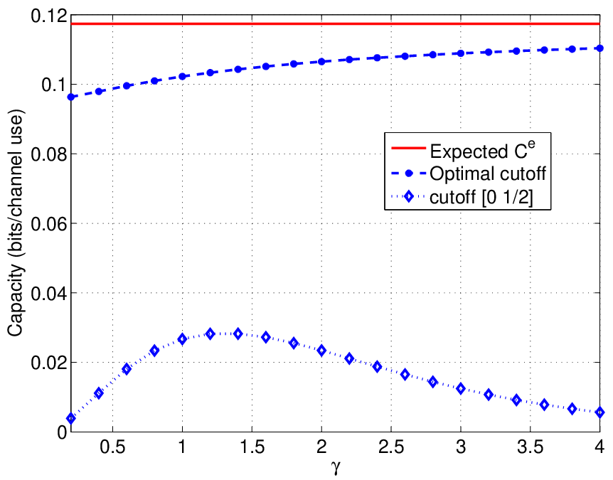
As an example, suppose that the crossover probability is uniformly distributed on . The Shannon capacity is limited by the worst channel state , giving . The capacity versus outage- is . To approximate the expected capacity, we solve for in (25) for each . It is seen that only for , where the two cutoff probabilities satisfy and . For the uniform distribution case, and , which demonstrates that it is unnecessary to use the channel all the time to achieve the expected capacity. In fact no information is sent for .


In Fig. 4 we plot the expected capacity, the outage- capacity, and the capacity versus outage-. Although the capacity versus outage- exceeds the expected capacity for some values of , the outage- capacity is always dominated by the expected capacity , since an outage- code is one of many possible codes for the expected capacity. Define cutoff outage probabilities and . Note that for all . In this range an outage code gives almost the same expected rate as a broadcast code.
In Fig. 5 we plot the rate used in each state by the expected capacity code and the capacity versus outage codes at outage probabilities , and . We see that the code for outage capacity achieves a constant rate for non-outage states and a rate otherwise. For this example, the incremental rates are nonzero only for . Therefore the code for expected capacity achieves a rate when . As decreases from to , the rate gradually increases from to bits per channel use, and stays at this constant level for . Since all channels are equally probable, the area under each curve is the expected rate of that strategy. The area under the expected capacity curve is the largest. The expected capacity curve is, in some places, lower than the curve for outage- capacity. Although the outage- code achieves a rate higher than the broadcast code for expected capacity when , the same code has decoding rate for all other channel states , giving a lower area under the total curve.
A potential advantage of the outage code is its simplicity. The transmission rate is fixed, so the code may be coupled with a conventional source code. The advantage of the expected capacity code is its higher expected rate. The code may be coupled with a multiresolution source code. It is not obvious which strategy yields better end-to-end coding performance in this example. In general, an expected rate code is required to achieve the optimal end-to-end distortion, but this code may use a rate vector on the boundary of the BC capacity region which is different from the rate vector used by the code that achieves the expected capacity [20].
The procedure to solve for the expected capacity is computationally intensive. In the above example, when looking for the optimal which leads to the expected capacity, we first identify the cutoff probabilities and then solve (25) for each in this range. We want to emphasize that the correct cutoff range, although seemingly a very coarse characterization of the optimal solution, is crucial to the expected rate. Consider some alternative approaches:
- •
Optimal cutoff with suboptimal :
(26) - •
Cutoff range :
(27)
The choice of makes convex (), linear () or concave () in both approaches. In Fig. 6, for ranges between and we plot the achievable expected rate using the cutoff range and suboptimal as in (27), the achievable expected rate using the optimal cutoff range and suboptimal as in (26), and the expected capacity of this channel. We observe that the optimal cutoff range yields an expected rate very close to , but the expected rate is clearly suboptimal if we use the cutoff range . By optimizing the cutoff range we actually capture most benefit of the expected-rate code as compared to the conventional code for Shannon capacity.
VII Source-Channel Coding and Separation
Channel capacity theorems deal with data transmission in a communication system. When extending the system to include the source of the data, we also need to consider the data compression problem. For the overall system, the end-to-end distortion is a well-accepted performance metric. When both the source and channel are stationary and ergodic, codes are usually designed to achieve the same end-to-end distortion level for any source sequence and channel realization. However, if the channel model is generalized to such scenarios as the composite channel above, it is natural to introduce generalized end-to-end distortion metrics such as the distortion versus outage and the expected distortion [46], similar to the development of alternative capacity definitions. These alternative distortion metrics are also considered in prior works [47, 48, 49, 19, 20, 50].
The renowned source-channel separation theorem [21, Theorem 2.4] asserts that a target distortion level is achievable if and only if the channel capacity exceeds the source rate distortion function , and a two-stage separate source-channel code suffices to meet the requirement44 4 The separation theorem for lossless transmission [2] can be regarded as a special case of zero distortion.. This theorem enables separate design of source and channel codes and guarantees the optimal performance. However, there are a few underlying assumptions: a single-user channel; a stationary ergodic source and channel; a single distortion level maintained for all transmission. It is known that the separation theorem fails if the first two assumptions do not hold [51, 27]. In fact, the end-to-end distortion metrics also dictate whether the source-channel separation holds for a communication system. In [46] we showed the direct part of source-channel separation under the distortion versus outage metric and established the converse for certain systems. On the contrary, source-channel separation does not hold under the expected distortion metric.
Source-channel separation implies that the operation of source and channel coding does not depend on the statistics of the counterpart. Meanwhile, the source and channel do need to communicate with each other through an interface, which is a single number in the classical separation theorem. For generalized source/channel models and distortion metrics, the interface is not necessarily a single rate and may allow multiple parameters to be agreed on between the source and channel encoders and decoders. As we expect a performance enhancement when source and channel exchange more information through more sophisticated interface, an interesting topic for future research would be to characterize the tradeoff between interface complexity and the achievable end-to-end performance [52].
VIII Conclusions
In view of the pessimistic nature of Shannon capacity for composite channels with CSIR, we propose alternative capacity definitions including capacity versus and expected capacity. These definitions lend insight to applications where side information at the receiver combined with appropriate source coding strategies can exploit these more flexible notions of capacity. We prove capacity theorems or bounds under each definition, and illustrate how expected achievable rates can be improved through examples of Gilbert-Elliot channels and a BSC with random crossover probabilities. While the use of capacity definitions inherently focuses our attention on achievable (expected) rates, we note that the existence of other meaningful measures of performance in the given coding environment. For example, since outage- codes are compatible with conventional source codes while expected capacity codes require multiresolution or multiple description codes, depending on whether or not the corresponding broadcast channel is degraded, the fact that the expected rate of the expected capacity code exceeds that of the outage- code does not guarantee lower end-to-end expected distortion. Furthermore, since a non-ergodic channel experiences a single ergodic mode for all time, there is some justification for performance measures that take the probability of suffering a very low-rate state into account. These topics provide a wealth of interesting questions for future research with some initial work presented in [20, 19, 46].
Appendix A Proof of Lemma 1
We prove if , and vice versa. Therefore equivalent probability measures of and imply identical Shannon capacity. The result is intuitive but we need to address a subtle technical issue: note that and are channel state distributions, while the Shannon capacity is defined through the information density distribution (7), which depends on both input and channel statistics.
Recall the Shannon capacity formula (8)
Denote by the input distribution that achieves the supremum in (8), and by the corresponding information density distribution. For arbitrary , we define
Notice that
| (28) | |||||
where we exchange the order of integral and limit according to dominant convergence theorem. From (28) we see that implies
Assuming , it follows that
Now define as the information density distribution of channel when evaluated at input , i.e.
Since is arbitrary, we see that implies , therefore
Appendix B Proof of Capacity versus Outage Theorem (12)
We first prove the achievability of the capacity versus outage theorem (12). Consider a fixed outage probability .
Encoding: For any input distribution , , and , generate the codebook by choosing , , i.i.d. according to the distribution .
Decoding: Define, for , the typical set as
For any channel output , we decode as follows:
- 1.
If for all , declare an outage;
- 2.
Otherwise, decode to the unique index such that . An error is declared if more than one such index exists.
Outage and Error Analysis: We recall the definition of events in (10) as
Assuming equiprobable inputs, the expected probability of an outage using the above scheme is:
where by definition of we have approaching for large enough. Likewise, when no outage is declared the expected probability of error is
| (29) | |||||
where the last inequality is obtained by noticing that implies
or equivalently
From (29) we see that for all and arbitrary , which completes our proof.
Next we prove the converse of the capacity versus outage theorem (12). Consider any sequence of codes with error probability and outage probability . Let represent the th code in the sequence, and assume a uniform input distribution
For each , let represent the decoding region associated with codeword and equal an analogy of the typical set, defined as
where is arbitrary. Then we have
since the decoding regions cannot overlap. Thus
which goes to zero if and only if by definition of .
Appendix C Proof of Theorem 1
C-A Mapping Broadcast Code to Expected-rate Code
We first show that any broadcast code can be mapped to an expected-rate code, so
| (30) |
for any .
Given a BC code as defined in Definition 6, we represent each message in a binary format consisting of bits and concatenate these bits to form an overall representation of bits, where
| (31) |
These information bits are indexed by the index set . We denote by the set of indices of the bits that correspond to the message set in the BC code. Note that may be empty for some , for different these index sets are mutually exclusive and
| (32) |
The BC code can be mapped to the following expected-rate code with transmit rate given by (31). For any , the bits with define a corresponding message in the message set of the BC code. The encoder for the expected rate code satisfies
where the superscript and BC distinguishes the encoder of the expected-rate code and the broadcast code. For a state in the composite channel, the receiver decodes those information bits with indices in the set
| (33) |
and the decoding rate is . For the composite channel, the decoder output
is obtained by concatenating the binary representations of each , where and
is the decoder output of receiver in the broadcast channel. The decoding error probability for the expected-rate code in channel state is
where the error event for the broadcast code is defined in (15). Notice that
so the expected error probability
as , according to the BC code definition. Therefore the rate
is an achievable expected rate and (30) is proved.
C-B Mapping Expected-rate Code to Broadcast Code
Next we show that for any fixed ,
| (34) |
According to the definition of the expected capacity, there exists a sequence of codes such that
| (35) |
and . The transmitted information bits are indexed by . Since the transmitter and the receiver agree on the index set of those information bits that can be reliably decoded in each channel state , the transmitter can define, for each subset of channel states, the index set of those information bits decodable exclusively for channel states within , i.e.
where
is the complement index set of . Denote by the cardinality of . We observe that are mutually exclusive, the relationship (32) and (33) still hold and the decoding rate satisfies .
The expected-rate code can be mapped to the following BC code. Define the message set of the BC code as
in the sense that each message has the corresponding binary representation . The encoder for the BC code satisfies
where is obtained by concatenating the binary representations of each . When the composite channel is in state , the decoder output is
Since for any satisfying , we define the decoder output for receiver in the BC to be
where the binary representation of each can be obtained by the corresponding bits in .
The error event for receiver of the BC is defined in (15) with the error probability
and the overall error probability
By definition of the expected-rate capacity
Assuming each channel state occurs with strictly positive probability, i.e. , then implies
Therefore the code constructed above is a valid BC code, i.e. , and we conclude
| (36) | |||||
From (35) and (36) we see the inequality (34) is established. Since is arbitrary, Theorem 1 is a result of (30) and (34).
Appendix D Proof of (17)
Consider a two-user BC where the channel to each user is a BEC with erasure probability , , i.e. the conditional marginal distribution satisfies
Assuming , we observe that the BC is stochastically degraded since
where and for
Therefore the capacity region of the BEC-BC is the convex hull of the closure of all satisfying
| (37) |
for some joint distribution . Since the
cardinality of the random variable is bounded by
[1, p. 422] and the channel is symmetric with respect to
the alphabet and , we can take Bernoulli
and as the transition probability of a binary symmetric
channel with crossover probability . This stochastically degraded
BEC-BC together with the auxiliary
random variable is illustrated in Fig. 7.

The capacity region (37) is evaluated to be
| (38) |
where is the binary entropy function. Assuming the two ergodic components are equally probable in the composite channel, the achievable expected rate using a broadcast code is then
Appendix E Proof of Upper Bound for Expected Capacity
Denote by , , and , , the set of codewords and decoding regions corresponding to channel . We fix and define for each and
| (39) | |||||
where (39) follows from (6). Notice that for any with
| (40) | |||||
Furthermore we have
where the chain of inequalities follows from Fatou’s lemma, (40), and the code constraint . Since the probability must be non-negative, we conclude
almost surely (a.s.) in . Thus for any ,
occurs infinitely often a.s. Assuming is bounded by , we then have
also occurs infinitely often a.s. Since is arbitrary, we see that
occurs infinitely often for arbitrary , which gives us the upper bound (18) for expected capacity. Note that the expectation in the upper bound (18) is indeed , so the upper bound can also be proved using the standard technique of Fano’s inequality.
References
- [1] T. Cover and J. Thomas, Elements of Information Theory. Wiley & Sons, Inc., 1991.
- [2] C. Shannon, “A mathematical theory of communication,” Bell Sys. Tech. Journal, vol. 27, pp. 379–423, 623–656, July, Oct. 1948.
- [3] R. Dobrushin, “General formulation of Shannon’s main theorem in information theory,” Amer. Math. Soc. Trans., vol. 33, pp. 323–438, 1963.
- [4] K. Winkelbauer, “On the coding theorem for decomposable discrete information channels I,” Kybernetika, vol. 7, no. 2, pp. 109–123, 1971.
- [5] J. C. Kieffer, “A general formula for the capacity of stationary nonanticipatory channels,” Inform. Contr., vol. 26, no. 4, pp. 381–391, 1974.
- [6] R. Ahlswede, “The weak capacity of averaged channels,” Z. Wahrscheinlichkeitstheorie und Verw. Gebiete, vol. 11, pp. 61–73, 1968.
- [7] S. Verdú and T. S. Han, “A general formula for channel capacity,” IEEE Trans. Inform. Theory, vol. 40, no. 4, pp. 1147–1157, July 1994.
- [8] M. Effros and A. Goldsmith, “Capacity definitions and coding strategies for general channels with receiver side information,” in Proc. IEEE Int. Symp. Inform. Theory (ISIT), Cambridge MA, August 1998, p. 39.
- [9] T. S. Han, Information-Spectrum Method in Information Theory, ser. Applications of mathematics. New York, NY: Springer, 2003.
- [10] R. M. Gray, Entropy and Information Theory. New York: Springer-Verlag, 1990.
- [11] L. Ozarow, S. Shamai, and A. Wyner, “Information theoretical considerations for cellular mobile radio,” IEEE Trans. Veh. Tech., vol. 43, no. 2, pp. 359–378, May 1994.
- [12] G. Foschini and M. Gans, “On limits of wireless communications in a fading environment when using multiple antennas,” Wireless Personal Comm., vol. 6, pp. 311–335, March 1998.
- [13] A. Goldsmith, S. A. Jafar, N. Jindal, and S. Vishwanath, “Capacity limits of MIMO channels,” IEEE J. Sel. Areas Commun., vol. 21, no. 5, pp. 684–702, June 2003.
- [14] L. Zheng and D. N. C. Tse, “Diversity and multiplexing: a fundamental tradeoff in multiple antenna channels,” IEEE Trans. Inform. Theory, vol. 49, pp. 1073–1096, May 2003.
- [15] T. Cover, “Broadcast channels,” IEEE Trans. Inform. Theory, vol. 18, pp. 2–14, Jan. 1972.
- [16] S. Shamai(Shitz), “A broadcast strategy for the Gaussian slowly fading channel,” in Proc. IEEE Int. Symp. Inform. Theory (ISIT), Ulm Germany, June 1997, p. 150.
- [17] S. Shamai and A. Steiner, “A broadcast approach for a single-user slowly fading MIMO channel,” IEEE Trans. Inform. Theory, vol. 49, no. 10, pp. 2617–2635, Oct. 2003.
- [18] M. Effros, A. Goldsmith, and Y. Liang, “Capacity definitions of general channels with receiver side information,” in Proc. IEEE Int. Symp. Inform. Theory (ISIT), Nice, France, June 2007, pp. 921–925.
- [19] D. Gündüz and E. Erkip, “Joint source-channel codes for MIMO block-fading channels,” IEEE Trans. Inform. Theory, vol. 54, no. 1, pp. 116–134, Jan. 2008.
- [20] C. T. K. Ng, D. Gündüz, A. Goldsmith, and E. Erkip, “Minimum expected distortion in Gaussian layered broadcast coding with successive refinement,” in Proc. IEEE Int. Symp. Inform. Theory (ISIT), Nice, France, June 2007, pp. 2226–2230.
- [21] I. Csiszár and J. Körner, Information Theory: Coding Theorems for Discrete Memoryless Systems. New York: Academic Press, 1981.
- [22] D. Blackwell, L. Breiman, and A. Thomasian, “The capacity of a class of channels,” Ann. Math. Stat., vol. 30, pp. 1229–1241, 1959.
- [23] J. Wolfowitz, Coding theorems of information theory. New York: Springer-Verlag, 1964.
- [24] I. Csiszar and P. Narayan, “The capacity of the arbitrarily varying channel,” IEEE Trans. Inform. Theory, vol. 37, no. 1, pp. 18–26, Jan. 1991.
- [25] A. Feinstein, “A new basic theorem of information theory,” IRE Trans. Inform. Theory, vol. IT-4, pp. 2–22, 1954.
- [26] T. S. Han and S. Verdú, “Approximation theory of output statistics,” IEEE Trans. Inform. Theory, vol. 39, no. 3, pp. 752–772, May 1993.
- [27] S. Vembu, S. Verdú, and Y. Steinberg, “The source-channel separation theorem revisited,” IEEE Trans. Inform. Theory, vol. 41, no. 1, pp. 44–54, Jan. 1995.
- [28] R. B. Ash, Information Theory. New York: Interscience Publishers, 1965.
- [29] R. Durrett, Probability: Theory and Examples, 3rd ed. Belmont CA: Duxbury Press, 2005.
- [30] G. Caire and D. Tuninetti, “The throughput of hybrid-ARQ protocols for the Gaussian collision channel,” IEEE Trans. Inform. Theory, vol. 47, no. 5, pp. 1971–1988, May 2001.
- [31] T. Ghanim and M. C. Valenti, “The throughput of hybrid-ARQ in block fading under modulation constraints,” in Conf. on Inform. Sciences and Systems (CISS), Princeton NJ, March 2006, pp. 253–258.
- [32] M. Ancis and D. D. Giusto, “Reconstruction of missing blocks in JPEG picture transmission,” in Proc. IEEE Pacific Rim Conf. on Comm., Computers and Signal Processing, Victoria, BC, August 1999, pp. 288–291.
- [33] A. Goldsmith, Wireless Communications. New York NY: Cambridge University Press, 2005.
- [34] E. Telatar, “Capacity of multi-antenna Gaussian channels,” Euro. Trans. Telecomm. (ETT), vol. 10, no. 6, pp. 585–596, Nov. 1999.
- [35] A. El Gamal, “The capacity of a class of broadcast channels,” IEEE Trans. Inform. Theory, vol. 25, no. 2, pp. 166–169, March 1979.
- [36] R. Gallager, Information Theory and Reliable Communication. New York: Wiley, 1968.
- [37] G. Caire and S. Shamai(Shitz), “On the achievable throughput of a multiple-antenna Gaussian broadcast channel,” IEEE Trans. Inform. Theory, vol. 49, no. 7, pp. 1691–1706, July 2003.
- [38] S. Vishwanath, N. Jindal, and A. Goldsmith, “Duality, achievable rates, and sum-rate capacity of gaussian MIMO broadcast channels,” IEEE Trans. Inform. Theory, vol. 49, no. 10, pp. 2658–2668, Oct. 2003.
- [39] W. Yu and J. Cioffi, “Sum capacity of gaussian vector broadcast channels,” IEEE Trans. Inform. Theory, vol. 50, no. 9, pp. 1875–1892, Sep. 2004.
- [40] P. Viswanath and D. N. C. Tse, “Sum capacity of the vector Gaussian broadcast channels and uplink-downlink duality,” IEEE Trans. Inform. Theory, vol. 49, no. 8, pp. 1912–1921, August 2003.
- [41] H. Weingarten, Y. Steinberg, and S. Shamai(Shitz), “The capacity region of the Gaussian multiple-input multiple-output broadcast channel,” IEEE Trans. Inform. Theory, vol. 52, no. 9, pp. 3936–3964, Sept. 2006.
- [42] D. Gündüz and E. Erkip, “Source and channel coding for quasi-static fading channels,” in Proc. Asilomar Conf. Signals, Systems and Computers, Pacific Grove, CA, Nov. 2005, pp. 18–22.
- [43] M. Mushkin and I. Bar-David, “Capacity and coding for the Gillbert-Elliot channels,” IEEE Trans. Inform. Theory, vol. 35, no. 6, pp. 1277–1290, Nov. 1989.
- [44] P. Bergmans, “Random coding theorem for broadcast channels with degraded components,” IEEE Trans. Inform. Theory, vol. 19, no. 2, pp. 197–207, March 1973.
- [45] D. Luenberger, Optimization by vector space methods. New York NY: John Wiley & Sons, Inc., 1969.
- [46] Y. Liang, A. Goldsmith, and M. Effros, “Distortion metrics of composite channels with receiver side information,” in IEEE Inform. Theory Workshop (ITW), Lake Tahoe, CA, Sept. 2007, pp. 559–564.
- [47] S. Shamai, S. Verdú, and R. Zamir, “Systematic lossy source/channel coding,” IEEE Trans. Inform. Theory, vol. 44, no. 2, pp. 564–579, March 1998.
- [48] Z. Reznic, M. Feder, and R. Zamir, “Distortion bounds for broadcasting with bandwidth expansion,” IEEE Trans. Inform. Theory, vol. 52, no. 8, pp. 3778–3788, August 2006.
- [49] U. Mittal and N. Phamdo, “Hybrid digital-analog (HDA) joint source-channel codes for broadcasting and robust communications,” IEEE Trans. Inform. Thoery, vol. 48, no. 5, pp. 1082–1102, May 2002.
- [50] K. Zachariadis, M. Honig, and A. Katsaggelos, “Source fidelity over a two-hop fading channel,” in IEEE MilCom, Monterey CA, Nov. 2004, pp. 134–139.
- [51] T. Cover, A. El Gamal, and M. Salehi, “Muliple access channels with arbitrarily correlated sources,” IEEE Trans. Inform. Theory, vol. 26, no. 6, pp. 648–657, Nov. 1980.
- [52] Y. Liang, A. Goldsmith, and M. Effros, “Source-channel coding and separation for general communication systems,” To be submitted to IEEE Trans. Inform. Theory, April 2008.