A spectral solver for evolution problems with spatial $\mathbb{S}^{3}$ -topology

Florian Beyer Email: beyer@ann.jussieu.fr

Laboratoire Jacques-Louis Lions
Université Pierre et Marie Curie (Paris 6)
4 Place Jussieu, 75252 Paris, France

Abstract

We introduce a single patch collocation method in order to compute solutions of initial value problems of partial differential equations whose spatial domains are $3$ -spheres. Besides the main ideas, we discuss issues related to our implementation and analyze numerical test applications. Our main interest lies in cosmological solutions of Einstein’s field equations. Motivated by this, we also elaborate on problems of our approach for general tensorial evolution equations when certain symmetries are assumed. We restrict to $\mathrm{U(1)}$ - and Gowdy symmetry here.

1 Introduction

Numerical studies of initial value problems of partial differential equations on certain spatial domains have a long history both in basic research and in applied science, see for instance [6] and references therein. In particular, for applications in geometrical classical theories in physics, as for instance general relativity, Maxwell theory, but also Ricci flow (introduced e.g. in [39]), there are interesting applications where the spatial domain is a $3$ -sphere. In general relativity, spatial $\mathbb{S}^{3}$ -topology plays a particularly important role for the standard model of cosmology based on the spatially homogeneous and isotropic Friedmann-Robertson-Walker solutions (see for instance [22, 40]). Beyond those simple and, at least for certain matter fields, well-understood models with high symmetry, there exist several outstanding open problems; of particular outstanding interest and motivation for this work here are the strong cosmic censorship and BKL conjecture in Gowdy vacuum solutions of Einstein’s field equations for spatial $\mathbb{S}^{3}$ - or $\mathbb{S}^{1}\times\mathbb{S}^{2}$ -topologies [21, 25, 9, 18, 4, 36].

It is not straight forward to deal with “non-trivial” spatial topologies, such as $\mathbb{S}^{3}$ , numerically. Recall the well-known problems occurring at the coordinate axis in the case of standard cylindrical coordinates $(\rho,\phi,z)$ in $\mathbb{R}^{3}$ . These coordinates degenerate at the “axis” given by $\rho=0$ . In typical equations, this has the consequence that derivatives with respect to the azimuthal angle $\phi$ always come together with a factor $1/\rho$ . If $f$ is a smooth function on $\mathbb{R}^{3}$ , then a term like $1/\rho\,\partial_{\phi}f$ is well-behaved at the axis. However, when an equation with such terms is solved numerically, the “formal singularity” $1/\rho$ can cause numerical instabilities. Applications with axial symmetry have a great history in all over science. Just to name examples of numerical studies of axisymmetric problems in general relativity, we list [19, 8, 34]. In this paper, we will not be interested in axial symmetry, however, it is instructive to keep it in mind for the following reason. Let us assume that we cover a dense subset of $\mathbb{S}^{3}$ with one coordinate patch, for instance the Euler coordinates introduced below. Then it turns out that this leads, loosely speaking, to two “axes” on $\mathbb{S}^{3}$ , each of which with similar properties as the axis for cylindrical coordinates on $\mathbb{R}^{3}$ . Hence, we call this the “axis problem” also in the case of spatial $\mathbb{S}^{3}$ -topology.

Alternatively to this approach with one singular coordinate patch on the spatial domain, one can try a multipatch technique. The idea is to cover the spatial domain with several local regular coordinate patches. In general relativity, examples of implementations of the multipatch technique are [38, 11]; of particular interest for our work here are implementations based on spectral methods in [32, 35, 12]. In any case, the multipatch technique does not seem advantageous for the applications which we have in mind. First, its implementation is difficult, since one must find a stable and efficient way of guaranteeing the necessary communication between the local patches. Second, we are interested in cosmological solutions with symmetries, and in order to take full advantage of those, it is often a good idea to adapt the coordinates to the symmetries, even though this can mean that one has to deal with singular coordinate systems. We have decided to develop a single patch code based on the collocation method¹¹ 1 In this paper we will often speak sloppily of spectral or pseudospectral methods when we mean the collocation method. for the spatial discretization. It is general experience that such methods typically yield high accuracy [6]. Furthermore, a spectral single patch approach seems very natural from our geometric point of view, which we introduce in this paper. For the time discretization, we use the method of lines with a Runge Kutta integrator. Such a discretization technique for various spatial domains has a long history in computational physics, see for instance the references and examples in [6]. An alternative approach, which uses spectral discretization both in space and in time, has been reported on in [23]. However, to our knowledge, the case of spatial $\mathbb{S}^{3}$ -topology has not been studied yet.

Our aim is to find numerical solutions of systems of first order quasi-linear evolution PDEs, written schematically as

\partial_{t}f(t,x)+\sum_{i}(A^{i}(f,t,x)\cdot\nabla_{i})f(t,x)+B(t,x,f)=0.

(1)

Here, the unknown $f$ is a vector, the terms $B$ are vector valued, and $A^{i}$ and $\nabla_{i}$ represent a collection of matrices and spatial derivative operators, as explained in more detail later. The spatial domain, represented by the abstract coordinates $x$ , is $\mathbb{S}^{3}$ . We assume in the following, without further notice, that the initial value problem for such a system is well-posed, i.e. that for any choice of initial data in a given regularity class, there exists a unique solution $f$ locally in time, which depends continuously on the initial data in a well-defined manner. In our applications, ignoring the “axis problem” above for the moment, the operators $\nabla_{i}$ can be thought of as the spatial partial derivatives, the quantities $A^{i}$ as symmetric matrices, and all coefficients depend smoothly on their arguments. In this case, the system is symmetric hyperbolic, and well-posedness follows [26, 28]. In particular, when the initial data is smooth, then the solution is smooth until it breaks down. We remark, that in principle our approach applies to other forms of hyperbolicity for Eq. (1), or even parabolic systems.

We will often use the following equivalent geometric language. Namely, we say that we look for solutions of Eq. (1) on $\mathbb{R}\times\mathbb{S}^{3}$ , where time $t$ is interpreted as the canonical coordinate on the factor $\mathbb{R}$ of the manifold $\mathbb{R}\times\mathbb{S}^{3}$ , and the $t=const$ -hypersurfaces have $\mathbb{S}^{3}$ -topology. In this paper, we will often be concerned with the case when $f$ in Eq. (1) represents components of smooth tensor fields. Then we call Eq. (1) “tensorial equation”.

This paper is organized as follows: Section 2 is devoted to the description and discussion of our numerical technique. We show our geometric point of view which leads, in a natural way, to a single patch collocation discretization in space. We demonstrate that it allows a straight forward treatment of the “axis problem” mentioned above. Since we are interested, in particular, in tensorial equations, we discuss several related issues in Section 2.3. Namely, in order to express the tensor fields as collections of smooth functions we have decided to work with smooth global frames on $\mathbb{S}^{3}$ . The formulation of tensorial equations in terms of smooth global frames on $\mathbb{S}^{3}$ leads to certain problems in the presence of symmetries. Two particular classes of symmetries of our interest are discussed. For these sections, but indeed at many places of this paper, some background in differential geometry would be helpful, which can be obtained for instance from [22, 29]. In Section 2.4, we elaborate on our numerical infrastructure in general, and we discuss certain issues related to numerical stability which are present for spatial $\mathbb{S}^{3}$ -topology. In Section 3, we proceed as follows. First, we introduce the mathematical and physical background of our test application. Then we test the code in that setting and elaborate on numerical errors, stability and performance. Finally, in Section 4, we summarize and conclude. We comment briefly on possible problems when some of our special assumptions are dropped, point to open issues and list aspects for future work.

2 Geometric ideas and numerical implementation

2.1 Euler coordinates and the Euler map

In the following, we consider the $3$ -sphere $\mathbb{S}^{3}$ as the submanifold of $\mathbb{R}^{4}$ given by

\mathbb{S}^{3}:=\left\{(x_{1},x_{2},x_{3},x_{4})\in\mathbb{R}^{4}\,\left|\,\sum_{i=1}^{4}x_{i}^{2}=1\right.\right\}.

(2)

The Euler coordinates of $\mathbb{S}^{3}$ , also appearing as Euler angle parametrization, etc. in the literature, is the coordinate patch given by

	$\displaystyle\begin{split}x_{1}&=\cos\frac{\chi}{2}\cos\lambda_{1},\quad x_{2}=\cos\frac{\chi}{2}\sin\lambda_{1},\\ x_{3}&=\sin\frac{\chi}{2}\cos\lambda_{2},\quad x_{4}=\sin\frac{\chi}{2}\sin\lambda_{2},\end{split}$	(3a)
in terms of the coordinate functions $\chi\in[0,\pi]$ , $\lambda_{1},\lambda_{2}\in\left[0,2\pi\right[$ . We will rather use the coordinates $\{\chi,\rho_{1},\rho_{2}\}$ determined by
	$\lambda_{1}=(\rho_{1}+\rho_{2})/2,\quad\lambda_{2}=(\rho_{1}-\rho_{2})/2.$	(3b)

The Euler coordinates smoothly cover the dense subset of $\mathbb{S}^{3}$ given, when the points $\chi=0,\pi$ are taken away. We expect that other choices of coordinates with similar properties are also appropriate. Although the motivation for choosing the Euler coordinates stems from Gowdy symmetry, as becomes clearer later, they are robust enough for more general cases.

Certainly, the relations in Eq. (3) are well-defined for all $\chi,\rho_{1},\rho_{2}\in\mathbb{R}$ . This is also true when we consider $\chi,\rho_{1},\rho_{2}\in(\mathbb{R}\text{ mod }4\pi)$ . Geometrically, the Euler coordinates given by Eq. (3) can thus be interpreted as a smooth map from the $3$ -torus

\mathbb{T}^{3}:=(\mathbb{R}\text{ mod }4\pi)\times(\mathbb{R}\text{ mod }4\pi)\times(\mathbb{R}\text{ mod }4\pi)

to $\mathbb{S}^{3}$ , which we call the Euler map

\begin{split}&\Phi:\mathbb{T}^{3}\rightarrow\mathbb{S}^{3},\\ (\chi,\rho_{1},\rho_{2})\mapsto&\left(\cos\frac{\chi}{2}\cos\frac{\rho_{1}+\rho_{2}}{2},\quad\cos\frac{\chi}{2}\sin\frac{\rho_{1}+\rho_{2}}{2},\right.\\ &\left.\sin\frac{\chi}{2}\cos\frac{\rho_{1}-\rho_{2}}{2},\quad\sin\frac{\chi}{2}\sin\frac{\rho_{1}-\rho_{2}}{2}\right)\in\mathbb{S}^{3}.\end{split}

(4)

The Euler map $\Phi$ is even a diffeomorphism when we restrict it to e.g. $\chi\in]0,\pi[$ and restrict the image correspondingly. But at the points $\chi=0,\pi$ , the inverse is not well-defined. Note, that in the whole paper we will often make the canonical identification of the isomorphic groups $\mathrm{U(1)}$ , $\mathbb{S}^{1}$ , $(\mathbb{R}\text{ mod }2\pi)$ and $(\mathbb{R}\text{ mod }4\pi)$ , and henceforth not distinguish between them. However at this point, our definition of the map requires to stand on $4\pi$ -periodicity at least for the coordinate $\chi$ , but we come to the standard $2\pi$ -periodicity in a moment.

Let $f$ be a smooth function on $\mathbb{S}^{3}$ . In the following we consider $\tilde{f}:=f\circ\Phi$ , where $\Phi$ is the Euler map defined in Eq. (4). Hence $\tilde{f}$ is a smooth function on $\mathbb{T}^{3}$ . For simplicity, we write $f$ instead of $\tilde{f}$ , and often make no difference between the “original function $f$ on $\mathbb{S}^{3}$ ” and the “corresponding function $\tilde{f}$ on $\mathbb{T}^{3}$ ”. If necessary, in order to avoid confusions, we sometimes say that “ $f$ is a smooth function on $\mathbb{T}^{3}$ originating in a smooth function on $\mathbb{S}^{3}$ ”.

Motivated by this simple geometric relation given by the Euler map, our approach is the following one; the details are worked out in the subsequent sections. Our aim is to solve partial differential equations with a spatial domain $\mathbb{S}^{3}$ . Let us suppose that all coefficient functions and unknown functions, which we want to solve for, in the equation are smooth functions on $\mathbb{S}^{3}$ . Furthermore, suppose that all derivative operators stem from smooth globally defined vector fields on $\mathbb{S}^{3}$ . Since $\Phi$ becomes a diffeomorphism, when we restrict it to a dense subset of $\mathbb{S}^{3}$ , all these functions and vector fields correspond in a unique manner to smooth functions and vector fields on the corresponding subset of $\mathbb{T}^{3}$ . Hence, we can solve the equation as if it its spatial domain were $\mathbb{T}^{3}$ . However, because $\Phi$ is not a diffeomorphism globally, we have introduced formal singularities to the equations, analogous to the singularities at the axis of cylindrical coordinates on $\mathbb{R}^{3}$ discussed above. One main conclusion in the following sections is that the hypothesis, that all these quantities on $\mathbb{T}^{3}$ originate in smooth quantities on $\mathbb{S}^{3}$ , allow to regularize the formally singular behavior at those points. By all this, we will successfully make “ $\mathbb{S}^{3}$ periodic in all three spatial directions”, and can henceforth use spectral methods based on the standard Fourier basis for the spatial discretization of the equations.

In all of what follows, we will assume, for simplicity, that all functions involved do not depend on the coordinate $\rho_{2}$ . We call such functions $\mathrm{U(1)}$ -symmetric, and later we interpret this symmetry geometrically. The generalization of the following ideas is, however, straight forward. This assumption has the following nice property. Let $f$ be a smooth $\mathrm{U(1)}$ -symmetric function on $\mathbb{S}^{3}$ . Then $f\circ\Phi$ is $2\pi$ -periodic (instead of $4\pi$ -periodic) in $\chi$ and $\rho_{1}$ . This is so, because we can use the symmetry in $\rho_{2}$ to switch the signs of all terms in Eq. (4) consistently as needed. Hence, in the following, we only need to deal with the standard $2\pi$ -periodicity.

Note, that analogous spectral approaches for equations with spatial domains diffeomorphic to $\mathbb{S}^{2}$ have been implemented before, see for instance [2, 6] and references therein.

2.2 Analysis of Fourier series of given smooth functions on $\mathbb{S}^{3}$

Let $f$ be a given smooth $\mathrm{U(1)}$ -symmetric function on $\mathbb{S}^{3}$ . The corresponding function $f$ on $\mathbb{T}^{3}$ is smooth, and hence has a representation in terms of a Fourier series. We come back to the question of convergence of such a series later. At this stage, we want to assume that this Fourier series is finite, and, without loss of generality, with $N$ summands both in $\chi$ and $\rho_{1}$ . Since $f$ is $\mathrm{U(1)}$ -symmetric function, it is $2\pi$ -periodic in both $\chi$ and $\rho_{1}$ , as argued before. Let $f$ be real valued. Then it must be of the form

f(\chi,\rho_{1})=F_{0}(\chi)+2\,\text{Re}\sum_{p=1}^{N}F_{p}(\chi)e^{ip\rho_{1}}.

(5)

Here, $F_{0}(\chi)$ is a real valued function, and $F_{p}(\chi)$ is allowed to be complex for all $p\geq 1$ . In [3], we demonstrated that the properties of the Euler map under $\mathrm{U(1)}$ -symmetry implies
	$F_{p}(\chi)=\begin{cases}{\displaystyle 2\sum_{n=1}^{N}f_{n,p}\cos n\chi+f_{0,p}}&\text{for $p\geq 0$ even},\\ {\displaystyle-2i\sum_{n=1}^{N}f_{n,p}\sin n\chi}&\text{for $p>0$ odd},\end{cases}$	(6a)
for some, in general, complex coefficients $f_{n,p}$ ; only the coefficients for $p=0$ must be real. Some of the factors in these expressions are chosen for later convenience. Note, that in [3], the coordinates $(\chi,\rho_{1},\rho_{2})$ are defined slightly differently. For example, the function $\chi$ here must be substituted by $2\chi$ to compare to the expressions in [3]. In any case, we further find that for even $p>0$ , there are the “compatibility conditions”
	$f_{0,p}+2\sum_{n=1}^{N}f_{2n,p}=0,\quad\sum_{n=1}^{N}f_{2n-1,p}=0.$	(6b)

These originate in the fact that the functions $F_{p}(\chi)$ must vanish at the degenerated places $\chi=0,\pi$ for all $p>0$ . For odd $p$ , this is implied by the expression Eq. (6a) automatically, and hence there are no compatibility conditions. The corresponding expressions are more complicated, but analogous, when we give up $\mathrm{U(1)}$ -symmetry.

Now, we want to study what happens to the Fourier series of $f$ , when it is differentiated along a smooth tangent vector field on $\mathbb{S}^{3}$ . By this, we mean that the abstract derivative operator $\nabla_{i}$ in Eq. (1) is of the form $\nabla_{i}f=V^{\alpha}\partial_{x^{\alpha}}f$ for a smooth tangent vector field $V=V^{\alpha}\partial_{x^{\alpha}}$ on $\mathbb{S}^{3}$ . Here, our convention is that $x^{\alpha}$ represents three abstract spatial coordinates, which neither need be the Cartesian coordinates, nor the Euler coordinates used before. However, we will restrict to Euler coordinates in the following. Furthermore, we assume Einstein’s summation convention. The coefficients $V^{\alpha}$ are just functions on $\mathbb{S}^{3}$ which are not necessarily smooth when we consider the Euler coordinates. Of particular importance will be the following tangent vector fields, whose origin we explain later and which, with respect to the Euler coordinates, take the form


$\displaystyle Y_{1}$	$\displaystyle=2\sin\rho_{1}\,\partial_{\chi}+2\cos\rho_{1}\,\left(\cot\chi\,\partial_{\rho_{1}}-\csc\chi\,\partial_{\rho_{2}}\right),$	(7a)
$\displaystyle Y_{2}$	$\displaystyle=2\cos\rho_{1}\,\partial_{\chi}-2\sin\rho_{1}\,\left(\cot\chi\,\partial_{\rho_{1}}-\csc\chi\,\partial_{\rho_{2}}\right),$	(7b)
$\displaystyle Y_{3}$	$\displaystyle=2\partial_{\rho_{1}}.$	(7c)

The factors $2$ are chosen for consistency with our discussion in [3]. Now, as we explain later, any smooth vector field $V$ on $\mathbb{S}^{3}$ can be written as a linear combination $V=V^{a}Y_{a}$ with $V^{1}$ , $V^{2}$ , $V^{3}$ smooth functions on $\mathbb{S}^{3}$ . Hence, under the assumption that all differential operators in the equations stem from smooth vector fields on $\mathbb{S}^{3}$ , it follows for $\mathrm{U(1)}$ -symmetry, that all “formally singular” differential operators in our equations must be of the form $-F(\chi,\rho_{1})\cot\chi\partial_{\rho_{1}}$ , with $F$ some smooth function on $\mathbb{S}^{3}$ . Without the assumption of $\mathrm{U(1)}$ -symmetry, there can additionally be singular operators of the form $(F(\chi,\rho_{1},\rho_{2})/\sin\chi)\partial_{\rho_{2}}$ . This shows that the formally singular terms here are of the same type as in the “axis problem”. The differences to the case of cylindrical coordinates on $\mathbb{R}^{3}$ are twofold. First, in the case of $\mathbb{S}^{3}$ , we have two such “axes” simultaneously at $\chi=0$ and $\pi$ . Second, the axis itself is not topologically a line here, but a closed circle. In the following, we restrict our attention to the operator relevant to $\mathrm{U(1)}$ -symmetry $-\cot\chi\partial_{\rho_{1}}$ .

So, let $f$ be as before, and $g:=\partial_{\rho_{1}}f$ . Since $g$ is again a smooth $\mathrm{U(1)}$ -symmetric function on $\mathbb{S}^{3}$ with finite Fourier series, the analogue of Eqs. (5) and (6) holds with $F_{p}(\chi)$ substituted schematically by the function $G_{p}(\chi)$ . Then, for $\chi\not=0,\pi$ , we get,

	$\begin{split}&-\cot\chi\,G_{p}(\chi)\\ &=\begin{cases}{\displaystyle\begin{split}2\Biggl[\mathfrak{c}_{2,p}\sin\chi+\sum_{k=1}^{N}&\Bigl\{(\mathfrak{b}_{k,p}+\mathfrak{b}_{k+1,p})\sin 2k\chi\\ &+(\mathfrak{c}_{k+1,p}+\mathfrak{c}_{k+2,p})\sin(2k+1)\chi\Bigr\}\Biggr]\end{split}}&\text{for $p>0$ even},\\ {\displaystyle\begin{split}2i\Biggl[\mathfrak{b}_{1,p}+\sum_{r=1}^{N}\Bigl\{&(\mathfrak{c}_{r,p}+\mathfrak{c}_{r+1,p})\cos(2r-1)\chi\\ &+(\mathfrak{b}_{r,p}+\mathfrak{b}_{r+1,p})\cos 2r\chi\Bigr\}\Biggr]\end{split}}&\text{for $p>0$ odd}.\end{cases}\end{split}$	(8a)
Here, we define
	$\mathfrak{b}_{r,p}^{N}:=\sum_{n=r}^{N}g_{2n,p},\quad\mathfrak{c}_{r,p}:=\sum_{n=r}^{N}g_{2n-1,p}\quad\text{for }r\geq 1.$	(8b)

The computations leading to this result are described in [3]. This result means that, as soon as the Fourier coefficients of $\partial_{\rho_{1}}f$ are known, the Fourier coefficients of the complete “formally singular term” $-\cot\chi\,\partial_{\rho_{1}}f$ can be computed.

Now, let us consider the general case of a given smooth $\mathrm{U(1)}$ -symmetric function $f$ on $\mathbb{S}^{3}$ . The associated function on $\mathbb{T}^{3}$ has an infinite Fourier representation in a general, with rapidly decreasing coefficients $f_{n,p}$ . This is a standard result from Fourier analysis, which can be found in [37, 7]. This last property means that the modules of the Fourier coefficients is bounded by a uniform constant times any negative integer power of the two summation indices $n$ and $p$ . This property is often referred to as “exponential convergence”. It is a general fact under our conditions that the Fourier series converges pointwise absolutely and even uniformly. We find straight forwardly that the Fourier series of $f$ must be of the form given by Eqs. (6), setting $N\rightarrow\infty$ . The infinite series of the compatibility condition Eq. (6b) converges because the coefficients are rapidly decreasing.

Now consider the inverse question. Let a function be given on $\mathbb{T}^{3}$ , of the form of Eqs. (5) and (6), for $N=\infty$ with rapidly decreasing coefficients $f_{n,p}$ . The standard theory implies that the series converges pointwise absolutely and uniformly to a smooth function $f$ on $\mathbb{T}^{3}$ . However, does $f$ originate in a smooth function on $\mathbb{S}^{3}$ ? In general the answer is no, because the compatibility conditions Eq. (6b) are just necessary, but not sufficient for smoothness. Indeed, it is sufficient that for any $p$ , the function $F_{p}(\chi)$ is a smooth $2\pi$ -periodic function on $\mathbb{R}$ , which has a zero of order $p$ at $\chi=0$ and $\pi$ . In particular, each function $F_{p}(\chi)e^{ip\rho_{1}}$ then originates in a smooth function on $\mathbb{S}^{3}$ . The argument for proving that this implies that $f$ is a smooth function on $\mathbb{S}^{3}$ , uses the theorem about Fourier series on $\mathbb{S}^{3}$ in [37]. Namely one can show that under these assumptions, $f$ as a function on $\mathbb{S}^{3}$ can be represented as an infinite series of spin-weighted spherical harmonics with again rapidly decreasing coefficients.

Consider the derivative $g=\partial_{\rho_{1}}f$ . In particular, the formula for $-\cot\chi\,g$ in Eqs. (8) also holds in the limit $N\rightarrow\infty$ , and the series expressions there converge at least pointwise at all $\chi\not=0,\pi$ . The function $-\cot\chi\,\partial_{\rho_{1}}f$ is a smooth function on $\mathbb{T}^{3}$ because each $F_{p}(\chi)$ in Eq. (5) is a smooth $2\pi$ -periodic function in $\chi$ with appropriate zeros at the “singular places” $\chi=0,\pi$ . This is a nice result because it shows that Eq. (8) is meaningful at the singular locations, and hence allows to evaluate the formally singular term $-\cot\chi\,\partial_{\rho_{1}}f$ explicitly there, even in the limit $N\rightarrow\infty$ . However, we remark that $-\cot\chi\,\partial_{\rho_{1}}f$ does not originate in a smooth function on $\mathbb{S}^{3}$ , because Eqs. (8) is not consistent with Eq. (6). This is not a problem because the formally singular operator is only a part of a differential operator defined by a smooth vector field on $\mathbb{S}^{3}$ . Indeed, the result, when this “full” differential operator is applied to a smooth function, yields a smooth function on $\mathbb{S}^{3}$ .

2.3 Symmetry and related issues for tensorial equations

Before we discuss, how these results can be applied in practice, let us first consider some consequences for tensorial equations.

2.3.1 Smooth frames on $\mathbb{S}^{3}$

Recall, that one of our main assumptions is that, at any given instance of time, all unknowns and coefficients in the equations are smooth functions, and that all differential operators are determined by smooth globally defined vector fields on $\mathbb{S}^{3}$ . However, in order to turn tensorial equations into partial differential equations for smooth scalar functions, we need to introduce smooth frames on $\mathbb{S}^{3}$ . We would like to mention that an alternative way of treating tensorial equations on $\mathbb{S}^{3}$ in the case of Gowdy symmetry, see below, can be found in [18] for the case of spatial $\mathbb{S}^{1}\times\mathbb{S}^{2}$ -topology.

Let us recall some well-known facts. Let $\mathbb{S}^{3}$ be given as in Eq. (2). Assume the standard matrix representation of the Lie group $\mathrm{SU(2)}$ [37]. The map

\Psi:\mathbb{S}^{3}\rightarrow\mathrm{SU(2)},\quad(x_{1},x_{2},x_{3},x_{4})\mapsto\begin{pmatrix}x_{1}+ix_{2}&-x_{3}+ix_{4}\\ x_{3}+ix_{4}&x_{1}-ix_{2}\end{pmatrix}

is a diffeomorphism, which can be used to transport the group structure of $\mathrm{SU(2)}$ to $\mathbb{S}^{3}$ . Hence, both $\mathrm{SU(2)}$ and $\mathbb{S}^{3}$ can be considered as identical Lie groups via the map $\Psi$ . Thus, from the standard $\mathrm{SU(2)}$ group multiplication, we can define left and right translation maps,

L,R:\mathbb{S}^{3}\times\mathbb{S}^{3}\rightarrow\mathbb{S}^{3},\quad(u,v)\mapsto L_{u}(v):=uv,\quad(u,v)\mapsto R_{u}(v):=vu,

so that $L_{u}$ and $R_{u}$ are diffeomorphisms $\mathbb{S}^{3}\rightarrow\mathbb{S}^{3}$ for each point $u\in\mathbb{S}^{3}$ . Those maps can be employed to construct smooth global frames. First one chooses a basis of the tangent space at the unit element $e$ of the group. We choose the Pauli matrices with non-standard normalization

\tilde{Y}_{1}=\begin{pmatrix}0&i\\ i&0\end{pmatrix},\quad\tilde{Y}_{2}=\begin{pmatrix}0&-1\\ 1&0\end{pmatrix},\quad\tilde{Y}_{3}=\begin{pmatrix}i&0\\ 0&-i\end{pmatrix},

considered as elements of $T_{e}(\mathrm{SU(2)})$ . Then, one uses the push forward of $L_{u}$ or $R_{u}$ to transport this basis smoothly to any other point $u\in\mathrm{SU(2)}$

(Y_{a})_{u}:=(L_{u})_{*}(\tilde{Y}_{a}),\quad(Z_{a})_{u}:=(R_{u})_{*}(\tilde{Y}_{a}).

Clearly, $\{Y_{a}\}$ is $\mathrm{SU(2)}$ -left invariant while $\{Z_{a}\}$ is $\mathrm{SU(2)}$ -right invariant and both are smooth global frame fields on $\mathbb{S}^{3}$ . It is straight forward to check that they satisfy

{}[Y_{a},Y_{b}]=2\sum_{c=1}^{3}\epsilon^{\mathchoice{\makebox[4.33765pt][c]{$\displaystyle$}}{\makebox[4.33765pt][c]{$\textstyle$}}{\makebox[2.59009pt][c]{$\scriptstyle$}}{\makebox[1.85005pt][c]{$\scriptscriptstyle$}}\mathchoice{\makebox[3.51666pt][c]{$\displaystyle$}}{\makebox[3.51666pt][c]{$\textstyle$}}{\makebox[2.1029pt][c]{$\scriptstyle$}}{\makebox[1.50208pt][c]{$\scriptscriptstyle$}}\mathchoice{\makebox[3.57375pt][c]{$\displaystyle$}}{\makebox[3.57375pt][c]{$\textstyle$}}{\makebox[2.1205pt][c]{$\scriptstyle$}}{\makebox[1.51463pt][c]{$\scriptscriptstyle$}}}_{{a}{b}{c}}Y_{c},\quad{}[Z_{a},Z_{b}]=2\sum_{c=1}^{3}\epsilon^{\mathchoice{\makebox[4.33765pt][c]{$\displaystyle$}}{\makebox[4.33765pt][c]{$\textstyle$}}{\makebox[2.59009pt][c]{$\scriptstyle$}}{\makebox[1.85005pt][c]{$\scriptscriptstyle$}}\mathchoice{\makebox[3.51666pt][c]{$\displaystyle$}}{\makebox[3.51666pt][c]{$\textstyle$}}{\makebox[2.1029pt][c]{$\scriptstyle$}}{\makebox[1.50208pt][c]{$\scriptscriptstyle$}}\mathchoice{\makebox[3.57375pt][c]{$\displaystyle$}}{\makebox[3.57375pt][c]{$\textstyle$}}{\makebox[2.1205pt][c]{$\scriptstyle$}}{\makebox[1.51463pt][c]{$\scriptscriptstyle$}}}_{{a}{b}{c}}Z_{c},\quad[Y_{a},Z_{b}]=0,

(9)

where $\epsilon^{\mathchoice{\makebox[4.33765pt][c]{$\displaystyle$}}{\makebox[4.33765pt][c]{$\textstyle$}}{\makebox[2.59009pt][c]{$\scriptstyle$}}{\makebox[1.85005pt][c]{$\scriptscriptstyle$}}\mathchoice{\makebox[3.51666pt][c]{$\displaystyle$}}{\makebox[3.51666pt][c]{$\textstyle$}}{\makebox[2.1029pt][c]{$\scriptstyle$}}{\makebox[1.50208pt][c]{$\scriptscriptstyle$}}\mathchoice{\makebox[3.57375pt][c]{$\displaystyle$}}{\makebox[3.57375pt][c]{$\textstyle$}}{\makebox[2.1205pt][c]{$\scriptstyle$}}{\makebox[1.51463pt][c]{$\scriptscriptstyle$}}}_{{a}{b}{c}}$ is the totally antisymmetric symbol with $\epsilon^{\mathchoice{\makebox[3.98613pt][c]{$\displaystyle$}}{\makebox[3.98613pt][c]{$\textstyle$}}{\makebox[2.45pt][c]{$\scriptstyle$}}{\makebox[1.75pt][c]{$\scriptscriptstyle$}}\mathchoice{\makebox[3.98613pt][c]{$\displaystyle$}}{\makebox[3.98613pt][c]{$\textstyle$}}{\makebox[2.45pt][c]{$\scriptstyle$}}{\makebox[1.75pt][c]{$\scriptscriptstyle$}}\mathchoice{\makebox[3.98613pt][c]{$\displaystyle$}}{\makebox[3.98613pt][c]{$\textstyle$}}{\makebox[2.45pt][c]{$\scriptstyle$}}{\makebox[1.75pt][c]{$\scriptscriptstyle$}}}_{{1}{2}{3}}=1$ . Here, the brackets denote the Lie bracket. For $\{Y_{a}\}$ , we have already written the explicit expressions with respect to the Euler coordinates in Eqs. (7). For $\{Z_{a}\}$ , we have


$\displaystyle Z_{1}$	$\displaystyle=-2\sin\rho_{2}\,\partial_{\chi}-2\cos\rho_{2}\,\left(\cot\chi\,\partial_{\rho_{1}}-\csc\chi\,\partial_{\rho_{2}}\right),$	(10a)
$\displaystyle Z_{2}$	$\displaystyle=2\cos\rho_{2}\,\partial_{\chi}-2\sin\rho_{2}\,\left(\cot\chi\,\partial_{\rho_{1}}-\csc\chi\,\partial_{\rho_{2}}\right),$	(10b)
$\displaystyle Z_{3}$	$\displaystyle=2\partial_{\rho_{2}}.$	(10c)

On $\mathbb{R}\times\mathbb{S}^{3}$ with a time function $t$ , we assume that each $t=const$ -hypersurface is diffeomorphic to $\mathbb{S}^{3}$ with Euler coordinates $\{\chi,\rho_{1},\rho_{2}\}$ . Hence, on each of these surfaces, the expressions Eqs. (7) and (10) define the fields $\{Y_{a}\}$ and $\{Z_{a}\}$ . Geometrically, we thus have for all $a=1,2,3$

[\partial_{t},Y_{a}]=[\partial_{t},Z_{a}]=0.

Now we write an arbitrary globally defined smooth frame $\{e_{i}\}$ on $\mathbb{R}\times\mathbb{S}^{3}$ as follows. By $\{e_{i}\}$ we mean the collection of $4$ frame fields $\{e_{0},e_{1},e_{2},e_{3}\}$ . We set

	$e_{0}=\partial_{t},$	(11a)
and write,
	$e_{a}=e^{\mathchoice{\makebox[4.33765pt][c]{$\displaystyle$}}{\makebox[4.33765pt][c]{$\textstyle$}}{\makebox[2.59009pt][c]{$\scriptstyle$}}{\makebox[1.85005pt][c]{$\scriptscriptstyle$}}{b}}_{{a}\mathchoice{\makebox[3.51666pt][c]{$\displaystyle$}}{\makebox[3.51666pt][c]{$\textstyle$}}{\makebox[2.1029pt][c]{$\scriptstyle$}}{\makebox[1.50208pt][c]{$\scriptscriptstyle$}}}Y_{b},$	(11b)

where $(e^{\mathchoice{\makebox[4.33765pt][c]{$\displaystyle$}}{\makebox[4.33765pt][c]{$\textstyle$}}{\makebox[2.59009pt][c]{$\scriptstyle$}}{\makebox[1.85005pt][c]{$\scriptscriptstyle$}}{b}}_{{a}\mathchoice{\makebox[3.51666pt][c]{$\displaystyle$}}{\makebox[3.51666pt][c]{$\textstyle$}}{\makebox[2.1029pt][c]{$\scriptstyle$}}{\makebox[1.50208pt][c]{$\scriptscriptstyle$}}})$ is a smooth $3\times 3$ -matrix valued function with non-vanishing determinant on $\mathbb{S}^{3}$ . Our conventions for frames is that the index $0$ always corresponds to the “time frame vector” $e_{0}$ and $a,b,\ldots=1,2,3$ correspond to the “spatial frame vectors”. When we write indices $i,j,\ldots=0,\ldots,3$ , we mean both the time and spatial frame vectors. For a tensor field $S$ , say for example a covariant $2$ -tensor, we write $S_{ij}:=S(e_{i},e_{j})$ , $S_{ab}:=S(e_{a},e_{b})$ etc. We stress, that it is important to understand, that writing $e_{i}$ , does not mean the $i$ th component of a vector $e$ , but rather the $i$ th vector field of the frame $\{e_{i}\}$ .

2.3.2 Symmetry reductions of tensorial equations

Let $S$ be an arbitrary smooth tensor field on $\mathbb{R}\times\mathbb{S}^{3}$ . We say that $S$ is $\xi$ -invariant, provided $\mathcal{L}_{\xi}S=0$ everywhere. Here $\mathcal{L}_{\xi}$ denotes the Lie derivative along $\xi$ . The coefficients $S_{ij}$ of $S$ , with respect to an arbitrary frame $\{e_{i}\}$ , are constant along $\xi$ , if, and in general only if, $[\xi,e_{i}]=0$ . Now, suppose that the functions $S_{ij}$ of such a tensor are among the unknowns of the system of partial differential equations which we would like to solve. Often, we would like to exploit the symmetry of the unknowns and reduce the equations to some simpler form. If the unknown functions are constant along $\xi$ , such a reduction can be done directly, if $\xi$ has the meaning of a spatial coordinate vector field. Hence, in the following, we will be interested in frames such that $[\xi,e_{i}]=0$ ; in this case, we say that the frame is $\xi$ -invariant.

Let us consider special cases of interest for us. We have already introduced the notion of $\mathrm{U(1)}$ -symmetry for functions before. For general smooth tensor fields $S$ on $\mathbb{R}\times\mathbb{S}^{3}$ , we define it by the requirement that $S$ is $Z_{3}$ -invariant. One can define $\mathrm{U(1)}$ -symmetry more geometrically, but for the purpose of this paper, our definition is sufficient. The integral curves of $Z_{3}=\partial_{\rho_{2}}$ are circles. Hence the symmetry group is isomorphic to $\mathrm{U(1)}$ , which motivates the name. Now, it is straight forward to construct $Z_{3}$ -invariant frames $\{e_{i}\}$ . Namely, for the ansatz Eqs. (11), this requirement is equivalent to

\partial_{\rho_{2}}(e^{\mathchoice{\makebox[4.33765pt][c]{$\displaystyle$}}{\makebox[4.33765pt][c]{$\textstyle$}}{\makebox[2.59009pt][c]{$\scriptstyle$}}{\makebox[1.85005pt][c]{$\scriptscriptstyle$}}{b}}_{{a}\mathchoice{\makebox[3.51666pt][c]{$\displaystyle$}}{\makebox[3.51666pt][c]{$\textstyle$}}{\makebox[2.1029pt][c]{$\scriptstyle$}}{\makebox[1.50208pt][c]{$\scriptscriptstyle$}}})=0,

due to Eqs. (9). The consequence is, that both the frame matrix $(e^{\mathchoice{\makebox[4.33765pt][c]{$\displaystyle$}}{\makebox[4.33765pt][c]{$\textstyle$}}{\makebox[2.59009pt][c]{$\scriptstyle$}}{\makebox[1.85005pt][c]{$\scriptscriptstyle$}}{b}}_{{a}\mathchoice{\makebox[3.51666pt][c]{$\displaystyle$}}{\makebox[3.51666pt][c]{$\textstyle$}}{\makebox[2.1029pt][c]{$\scriptstyle$}}{\makebox[1.50208pt][c]{$\scriptscriptstyle$}}})$ and the frame components of all tensor fields, which are $Z_{3}$ -invariant, are constant along $\rho_{2}$ , and hence are $\mathrm{U(1)}$ -symmetric functions. Provided, our equations are formulated with respect to functions with this property only, the spatial domain reduces to that of the coordinates $\{\chi,\rho_{1}\}$ . We refer to this as the $2+1$ -reduced equations.

Another symmetry assumption of interest is Gowdy symmetry with two spatial symmetry vector fields. We say, that a tensor field is Gowdy symmetric, if it is $\mathrm{U(1)}$ -symmetric and additionally $Y_{3}$ -invariant. Again, this definition can be made more geometric. In any case, let us suppose that a frame field $\{e_{i}\}$ , obeying Eqs. (11) and $[Z_{3},e_{i}]=0$ , is given as before. Now, it turns out, as argued in [3], that the assumption that $\{e_{i}\}$ is a smooth globally defined $Z_{3}$ -invariant frame on $\mathbb{S}^{3}$ , does not allow that it is $Y_{3}$ -invariant in addition. Hence, although we can find a frame such that the frame components of arbitrary Gowdy symmetric tensor fields are constant along $\rho_{2}$ , it is not possible to achieve that in addition they are constant along $\rho_{1}$ ; recall $Y_{3}=\partial_{\rho_{1}}$ . Thus, even if we assumed Gowdy symmetry, the spatial domain of our equations would not reduce directly to that of the coordinate $\chi$ , i.e. not to $1+1$ dimensions. This difficulty is a consequence of our assumption that the frame is smooth globally on the manifold; if we allowed the frame to become singular at some places, then the situation would be different. However, we would get other problems due to the additional singularities.

Nevertheless, even under these assumptions, it is possible to perform the following “indirect” reduction of the equations to $1+1$ dimensions in the case of Gowdy symmetry. For the frame components of any smooth tensor field $S$ , for example in the case of a covariant $2$ -tensor, which is $Y_{3}$ -invariant, we find

Y_{3}(S_{ij})=S_{i^{\prime}j}T^{\mathchoice{\makebox[2.82928pt][c]{$\displaystyle$}}{\makebox[2.82928pt][c]{$\textstyle$}}{\makebox[1.68811pt][c]{$\scriptstyle$}}{\makebox[1.2058pt][c]{$\scriptscriptstyle$}}{i^{\prime}}}_{{i}\mathchoice{\makebox[4.67677pt][c]{$\displaystyle$}}{\makebox[4.67677pt][c]{$\textstyle$}}{\makebox[3.1506pt][c]{$\scriptstyle$}}{\makebox[2.66829pt][c]{$\scriptscriptstyle$}}}+S_{ij^{\prime}}T^{\mathchoice{\makebox[3.71356pt][c]{$\displaystyle$}}{\makebox[3.71356pt][c]{$\textstyle$}}{\makebox[2.29834pt][c]{$\scriptstyle$}}{\makebox[1.64166pt][c]{$\scriptscriptstyle$}}{j^{\prime}}}_{{j}\mathchoice{\makebox[5.56105pt][c]{$\displaystyle$}}{\makebox[5.56105pt][c]{$\textstyle$}}{\makebox[3.76083pt][c]{$\scriptstyle$}}{\makebox[3.10416pt][c]{$\scriptscriptstyle$}}}

(12)

with

T^{\mathchoice{\makebox[2.82928pt][c]{$\displaystyle$}}{\makebox[2.82928pt][c]{$\textstyle$}}{\makebox[1.68811pt][c]{$\scriptstyle$}}{\makebox[1.2058pt][c]{$\scriptscriptstyle$}}{i^{\prime}}}_{{i}\mathchoice{\makebox[4.67677pt][c]{$\displaystyle$}}{\makebox[4.67677pt][c]{$\textstyle$}}{\makebox[3.1506pt][c]{$\scriptstyle$}}{\makebox[2.66829pt][c]{$\scriptscriptstyle$}}}e_{i^{\prime}}:=[Y_{3},e_{i}].

Under our assumptions for the frame Eqs. (11), we see that

T^{\mathchoice{\makebox[3.98613pt][c]{$\displaystyle$}}{\makebox[3.98613pt][c]{$\textstyle$}}{\makebox[2.45pt][c]{$\scriptstyle$}}{\makebox[1.75pt][c]{$\scriptscriptstyle$}}{i^{\prime}}}_{{0}\mathchoice{\makebox[4.67677pt][c]{$\displaystyle$}}{\makebox[4.67677pt][c]{$\textstyle$}}{\makebox[3.1506pt][c]{$\scriptstyle$}}{\makebox[2.66829pt][c]{$\scriptscriptstyle$}}}=0,\quad T^{\mathchoice{\makebox[2.82928pt][c]{$\displaystyle$}}{\makebox[2.82928pt][c]{$\textstyle$}}{\makebox[1.68811pt][c]{$\scriptstyle$}}{\makebox[1.2058pt][c]{$\scriptscriptstyle$}}{0}}_{{i}\mathchoice{\makebox[3.98613pt][c]{$\displaystyle$}}{\makebox[3.98613pt][c]{$\textstyle$}}{\makebox[2.45pt][c]{$\scriptstyle$}}{\makebox[1.75pt][c]{$\scriptscriptstyle$}}}=0.

For the spatial components, one has

T^{\mathchoice{\makebox[4.33765pt][c]{$\displaystyle$}}{\makebox[4.33765pt][c]{$\textstyle$}}{\makebox[2.59009pt][c]{$\scriptstyle$}}{\makebox[1.85005pt][c]{$\scriptscriptstyle$}}{a^{\prime}}}_{{a}\mathchoice{\makebox[6.18513pt][c]{$\displaystyle$}}{\makebox[6.18513pt][c]{$\textstyle$}}{\makebox[4.05258pt][c]{$\scriptstyle$}}{\makebox[3.31255pt][c]{$\scriptscriptstyle$}}}=Y_{3}(e^{\mathchoice{\makebox[4.33765pt][c]{$\displaystyle$}}{\makebox[4.33765pt][c]{$\textstyle$}}{\makebox[2.59009pt][c]{$\scriptstyle$}}{\makebox[1.85005pt][c]{$\scriptscriptstyle$}}{c}}_{{a}\mathchoice{\makebox[3.57375pt][c]{$\displaystyle$}}{\makebox[3.57375pt][c]{$\textstyle$}}{\makebox[2.1205pt][c]{$\scriptstyle$}}{\makebox[1.51463pt][c]{$\scriptscriptstyle$}}})f^{\mathchoice{\makebox[3.57375pt][c]{$\displaystyle$}}{\makebox[3.57375pt][c]{$\textstyle$}}{\makebox[2.1205pt][c]{$\scriptstyle$}}{\makebox[1.51463pt][c]{$\scriptscriptstyle$}}{a^{\prime}}}_{{c}\mathchoice{\makebox[6.18513pt][c]{$\displaystyle$}}{\makebox[6.18513pt][c]{$\textstyle$}}{\makebox[4.05258pt][c]{$\scriptstyle$}}{\makebox[3.31255pt][c]{$\scriptscriptstyle$}}}+2e^{\mathchoice{\makebox[4.33765pt][c]{$\displaystyle$}}{\makebox[4.33765pt][c]{$\textstyle$}}{\makebox[2.59009pt][c]{$\scriptstyle$}}{\makebox[1.85005pt][c]{$\scriptscriptstyle$}}{c}}_{{a}\mathchoice{\makebox[3.57375pt][c]{$\displaystyle$}}{\makebox[3.57375pt][c]{$\textstyle$}}{\makebox[2.1205pt][c]{$\scriptstyle$}}{\makebox[1.51463pt][c]{$\scriptscriptstyle$}}}\epsilon^{\mathchoice{\makebox[3.98613pt][c]{$\displaystyle$}}{\makebox[3.98613pt][c]{$\textstyle$}}{\makebox[2.45pt][c]{$\scriptstyle$}}{\makebox[1.75pt][c]{$\scriptscriptstyle$}}\mathchoice{\makebox[3.57375pt][c]{$\displaystyle$}}{\makebox[3.57375pt][c]{$\textstyle$}}{\makebox[2.1205pt][c]{$\scriptstyle$}}{\makebox[1.51463pt][c]{$\scriptscriptstyle$}}{d}}_{{3}{c}\mathchoice{\makebox[4.16287pt][c]{$\displaystyle$}}{\makebox[4.16287pt][c]{$\textstyle$}}{\makebox[2.55038pt][c]{$\scriptstyle$}}{\makebox[1.8217pt][c]{$\scriptscriptstyle$}}}f^{\mathchoice{\makebox[4.16287pt][c]{$\displaystyle$}}{\makebox[4.16287pt][c]{$\textstyle$}}{\makebox[2.55038pt][c]{$\scriptstyle$}}{\makebox[1.8217pt][c]{$\scriptscriptstyle$}}{a^{\prime}}}_{{d}\mathchoice{\makebox[6.18513pt][c]{$\displaystyle$}}{\makebox[6.18513pt][c]{$\textstyle$}}{\makebox[4.05258pt][c]{$\scriptstyle$}}{\makebox[3.31255pt][c]{$\scriptscriptstyle$}}}.

The matrix $(f^{\mathchoice{\makebox[3.57375pt][c]{$\displaystyle$}}{\makebox[3.57375pt][c]{$\textstyle$}}{\makebox[2.1205pt][c]{$\scriptstyle$}}{\makebox[1.51463pt][c]{$\scriptscriptstyle$}}{a}}_{{c}\mathchoice{\makebox[4.33765pt][c]{$\displaystyle$}}{\makebox[4.33765pt][c]{$\textstyle$}}{\makebox[2.59009pt][c]{$\scriptstyle$}}{\makebox[1.85005pt][c]{$\scriptscriptstyle$}}})$ is defined here as the inverse of the matrix $(e^{\mathchoice{\makebox[4.33765pt][c]{$\displaystyle$}}{\makebox[4.33765pt][c]{$\textstyle$}}{\makebox[2.59009pt][c]{$\scriptstyle$}}{\makebox[1.85005pt][c]{$\scriptscriptstyle$}}{c}}_{{a}\mathchoice{\makebox[3.57375pt][c]{$\displaystyle$}}{\makebox[3.57375pt][c]{$\textstyle$}}{\makebox[2.1205pt][c]{$\scriptstyle$}}{\makebox[1.51463pt][c]{$\scriptscriptstyle$}}})$ . As soon as we fix the transport of the frame in time, we can compute the time derivative of the matrix $(T^{\mathchoice{\makebox[4.33765pt][c]{$\displaystyle$}}{\makebox[4.33765pt][c]{$\textstyle$}}{\makebox[2.59009pt][c]{$\scriptstyle$}}{\makebox[1.85005pt][c]{$\scriptscriptstyle$}}{a^{\prime}}}_{{a}\mathchoice{\makebox[6.18513pt][c]{$\displaystyle$}}{\makebox[6.18513pt][c]{$\textstyle$}}{\makebox[4.05258pt][c]{$\scriptstyle$}}{\makebox[3.31255pt][c]{$\scriptscriptstyle$}}})$ ; we do this for a particular example in Section 3.1. In general, we can expect that these evolution equations for the matrix $(T^{\mathchoice{\makebox[4.33765pt][c]{$\displaystyle$}}{\makebox[4.33765pt][c]{$\textstyle$}}{\makebox[2.59009pt][c]{$\scriptstyle$}}{\makebox[1.85005pt][c]{$\scriptscriptstyle$}}{a^{\prime}}}_{{a}\mathchoice{\makebox[6.18513pt][c]{$\displaystyle$}}{\makebox[6.18513pt][c]{$\textstyle$}}{\makebox[4.05258pt][c]{$\scriptstyle$}}{\makebox[3.31255pt][c]{$\scriptscriptstyle$}}})$ are non-trivial. In any case, the idea for the “indirect” reduction to $1+1$ in the Gowdy case is the following: first, substitute the $Y_{3}$ -derivatives of all tensor field components in the equations by means of Eq. (12). Second, append the evolution equations for the matrix $(T^{\mathchoice{\makebox[4.33765pt][c]{$\displaystyle$}}{\makebox[4.33765pt][c]{$\textstyle$}}{\makebox[2.59009pt][c]{$\scriptstyle$}}{\makebox[1.85005pt][c]{$\scriptscriptstyle$}}{a^{\prime}}}_{{a}\mathchoice{\makebox[6.18513pt][c]{$\displaystyle$}}{\makebox[6.18513pt][c]{$\textstyle$}}{\makebox[4.05258pt][c]{$\scriptstyle$}}{\makebox[3.31255pt][c]{$\scriptscriptstyle$}}})$ to the system of equations and, third, evaluate the equations only at $\rho_{1}=0$ . Then, with respect to the Euler coordinates, all unknowns only depend on $t$ and $\chi$ , and the evolution system is closed. Note, however, that it depends on the properties of the evolution equations of $(T^{\mathchoice{\makebox[4.33765pt][c]{$\displaystyle$}}{\makebox[4.33765pt][c]{$\textstyle$}}{\makebox[2.59009pt][c]{$\scriptstyle$}}{\makebox[1.85005pt][c]{$\scriptscriptstyle$}}{a^{\prime}}}_{{a}\mathchoice{\makebox[6.18513pt][c]{$\displaystyle$}}{\makebox[6.18513pt][c]{$\textstyle$}}{\makebox[4.05258pt][c]{$\scriptstyle$}}{\makebox[3.31255pt][c]{$\scriptscriptstyle$}}})$ , whether the resulting system of evolution equations yields a well-posed initial value problem. In the example, which we discuss later, this is the case.

We remark that under the assumption of $\mathrm{U(1)}$ -symmetry, all results obtained here also hold for spatial $\mathbb{S}^{1}\times\mathbb{S}^{2}$ -topology. We do not elaborate on this further; a discussion is given in [5].

2.4 Numerical implementation

2.4.1 Discretization and our numerical infrastructure

In order to compute approximate solutions of our system of partial differential equations Eq. (1) by means of a computer, we need to discretize the equations and the unknowns. Our analysis before based on Fourier series suggests spectral discretization [7, 6] in space with the standard trigonometric basis. We follow most of the conventions in [6]. In order to keep the presentation as short as possible here, we do not write down formulas wherever we follow the standard conventions. In particular, we use the collocation method. For the spatial grid in any of the spatial dimensions, referred to as $x$ , we set

x_{k}=(k+\mu)\frac{2\pi}{N},\quad k=0,\ldots,N-1,

(13)

where $N$ is the number of grid points in the chosen spatial direction. The quantity $\mu\in[0,1[$ is a shift quantity. For the standard collocation method which we use, the quantity $N$ must be odd.

For simplicity we use the so-called partial summation algorithm [6] for computing the discrete Fourier transforms (DFT) so far; however, we plan to switch to the Fast Fourier Transform algorithm (FFT) [10, 33], in order to optimize performance for high spatial resolutions.

This discretization of the equations and unknowns in space yields a system of ordinary differential equation (ODE) in time for the spectral coefficients of the unknowns, or equivalently for the values of all unknown functions at the spatial grid points. This system of ODEs is called the semi-discrete system. In order to solve this numerically, one must discretize time as well. For this, we have implemented a couple of Runge Kutta (RK) variations described in [33]; namely, first, the non-adaptive $4$ th order RK scheme, second, the $4$ th order “double-step-adaption” RK scheme and, third, the adaptive $5$ th order “embedded” RK scheme. For those schemes, the time adaption is always “global in space”, namely, at a given time the maximal estimated error at all spatial points is taken. The parameter $\eta$ is the desired accuracy, according to Eq. (16.2.7) in [33], where it is called $\Delta_{0}$ . The lower its value, the stronger is the tendency of the adaption scheme to decrease the time step $h$ . For practical reasons, we also define a minimal time step $h_{min}$ , so that the adaption scheme is prevented from reaching unpractically small values of $h$ .

A sophisticated discussion of errors and convergence in such discretization approaches is given in [7]. We will not elaborate on this, in general, very complicated problem analytically. Instead, we will investigate errors and convergence in our test applications empirically in Section 3.2. The positive experience, which people have gathered over many years of research with the collocation method, is summarized in Boyd’s empirical “assumption of equal errors” [6], which we decided to rely on in our numerical work.

It is clear that many classes of problems require adaptive techniques for the spatial resolution. One particular effect for underresolved numerical solutions obtained by the collocation method is aliasing. We have not yet implemented any of the explicit antialiasing recipes, given for instance in [6]. Instead, we use the following simple global spatial adaption technique so far. At each time step of the numerical evolution, the program computes the Fourier transform of one representative unknown function; which one is chosen requires some experiments. In our applications, where symmetry implies that only one spatial direction is significant, it is then sufficient to do the following. From the spectral coefficients of this unknown, the code determines the “power” of the upper third of the frequency spectrum with respect to the significant spatial direction, divided by the total power. It is straight forward to generalized this to more general situations. By “power” we mean the sum over the squares of the modulus of the Fourier coefficients. We call the result of this computation the “adaption norm” $\mathrm{Norm}^{(\textit{adapt})}$ . Besides adaption itself, this “norm” can also be thought of as a measure for the aliasing error. When, during the numerical evolution, $\mathrm{Norm}^{(\textit{adapt})}$ exceeds a prescribed threshold value, the code stops automatically, interpolates all quantities to a higher spatial resolution and continues the run. In each of these adaption steps, we have found it to be reasonable to almost double the spatial resolution. In any case, note that this is a primitive adaption method, since it is “global in space”. In particular, for solutions, which develop sharp localized features, a local adaption method in space would be more desirable. This is a future work project. However, even Gowdy spikes have been treated with our much simpler method in [3].

Let us, furthermore, mention the possibility of the Intel Fortran compiler [24] on Intel CPUs, which we have worked on exclusively up to now, to switch from the standard machine supported number representation called “double precision” with round-off errors of the order $10^{-16}$ to software emulated “quad precision” with round-off errors of the order $10^{-32}$ . Indeed, this possibility is exploited in our applications, as is discussed later.

2.4.2 Practical issues for spatial $\mathbb{S}^{3}$ -topology

In this paper, we discuss two codes for spatial $\mathbb{S}^{3}$ -topology which both use the infrastructure above, but with slight differences. For one of the codes, we assume $\mathrm{U(1)}$ -symmetry with a choice of orthonormal frame reducing the equations to two spatial dimensions; we call this code the $2+1$ -code. For the other code, which we call $1+1$ -code, we assume Gowdy symmetry, and suppose that the indirect reduction to one spatial dimension described before leads to a well-posed initial value formulation. The particular equations which we implement and study in both cases are discussed in Section 3.1.

In order to apply the results, which we obtained for the properties of Fourier series of smooth $\mathrm{U(1)}$ -symmetric functions on $\mathbb{S}^{3}$ in Section 2.2 in our discretization approach, we assume that for any choice of resolution, the solution of the corresponding discretized equations originates in smooth functions on $\mathbb{S}^{3}$ . Let us suppose, that our evolution equations have the property, that if the initial data of the continuum problem is smooth, then the corresponding solution of the continuum equations is smooth. For instance, this is the case for symmetric hyperbolic systems. Then, if the initial data is approximated by functions, which originate in smooth functions on $\mathbb{S}^{3}$ , and, if all our assumptions about the coefficients and derivative operators in the equations before hold, then the solution of the discretized originates in smooth functions on $\mathbb{S}^{3}$ for any resolution. This is at least true, as far as we can neglect errors caused by aliasing and the finite number representation in our computer. Let us assume just for a moment, that these errors can be neglected. In particular, Eq. (8) can be applied to the $2+1$ -code directly. For the $1+1$ -code, we need one further observation, since the equations are only evaluated at $\rho_{1}=0$ , and hence there is no information about even and odd Fourier modes with respect to $\rho_{1}$ . Namely, due to Eq. (6a), all coefficients associated with $\cos$ -modes with respect to $\chi$ must correspond to an even mode with respect to $\rho_{1}$ . Analogously, all coefficients associated with $\sin$ -modes with respect to $\chi$ must correspond to an odd mode with respect to $\rho_{1}$ . This information is sufficient to use Eqs. (8) as in the $2+1$ -case. Now, for even $p>0$ , there are two ways of computing the coefficients $\mathfrak{b}_{r,p}^{N}$ and $\mathfrak{c}_{r,p}^{N}$ of the formally singular terms. Namely, due to the compatibility conditions Eqs. (6b), we can write both

\mathfrak{b}_{r,p}^{N}=\sum_{n=r}^{N/2}g^{N}_{2n,p}=-\frac{1}{2}g^{N}_{0,p}-\sum_{n=1}^{r-1}g^{N}_{2n,p},\quad\mathfrak{c}_{r,p}^{N}=\sum_{n=r}^{N/2}g^{N}_{2n-1,p}=-\sum_{n=1}^{r-1}g^{N}_{2n-1,p}.

For odd $p$ , there is only one way of writing these coefficients. Although each pair is equivalent in exact computations, there can be a difference numerically. We refer to the first way of computing these coefficients as “up-to-down”, since we need the information of all high frequencies to compute the low frequency coefficients recursively. The second variant is called “down-to-up”, since the information from low frequency coefficients is used to compute the high frequency coefficients recursively.

A priori, both ways have the potential to amplify numerical instabilities. In particular, although the solution originates in smooth functions on $\mathbb{S}^{3}$ at one time of the evolution, this together with round-off errors and aliasing can cause a drift, so that the form given by Eqs. (6) are violated eventually. We have not yet built the special structure of the Fourier series into our numerical infrastructure. Thus, it is possible, that such errors accumulate, such that, after some time of evolution, the numerical solution does not represent a smooth solution on $\mathbb{S}^{3}$ anymore. Indeed, we found in our numerical experiments with the $2+1$ -code in [3], that, without precautions, the numerical solution typically drifts away strongly for both the up-to-down and down-to-up method. We were not able to pin-point the problem. However, for the down-to-up method, it turns out to be sufficient, after each time step, to set all those Fourier coefficients to zero explicitly, which are supposed to vanish according to Eq. (6a). With this manipulation, the numerical evolution becomes stable. In particular, Eq. (6b) stays satisfied within reasonable error limits, and the code is convergent and able to reproduce explicitly known solutions. The up-to-down method, however, we were not able to stabilize.

We can expect that similar practical issues exist for the $1+1$ -code. Here, however, we must proceed slightly differently, since the form given by Eqs. (6) cannot be enforced explicitly. In order to control the smoothness of the numerical solution nevertheless, the idea is to control the unknowns directly at the coordinate singularities $\chi=0,\pi$ in terms of ‘‘boundary conditions’’²² 2 This is the terminology from [18]. We use it despite the fact that there are no geometrical boundaries at $\chi=0,\pi$ .. Let the frame $\{e_{i}\}$ be $Z_{3}$ -invariant as before, and let $S$ be one of the unknown $Z_{3}$ -invariant tensor fields. Since $Y_{3}=\pm Z_{3}$ on the symmetry axes, one obtains $Y_{3}(S_{ij})=0$ there. Exploiting this information by means of Eq. (12), implies a homogeneous linear algebraic “boundary system”, which yields the “boundary conditions” for $S$

S_{i^{\prime}j}T^{\mathchoice{\makebox[2.82928pt][c]{$\displaystyle$}}{\makebox[2.82928pt][c]{$\textstyle$}}{\makebox[1.68811pt][c]{$\scriptstyle$}}{\makebox[1.2058pt][c]{$\scriptscriptstyle$}}{i^{\prime}}}_{{i}\mathchoice{\makebox[4.67677pt][c]{$\displaystyle$}}{\makebox[4.67677pt][c]{$\textstyle$}}{\makebox[3.1506pt][c]{$\scriptstyle$}}{\makebox[2.66829pt][c]{$\scriptscriptstyle$}}}+S_{ij^{\prime}}T^{\mathchoice{\makebox[3.71356pt][c]{$\displaystyle$}}{\makebox[3.71356pt][c]{$\textstyle$}}{\makebox[2.29834pt][c]{$\scriptstyle$}}{\makebox[1.64166pt][c]{$\scriptscriptstyle$}}{j^{\prime}}}_{{j}\mathchoice{\makebox[5.56105pt][c]{$\displaystyle$}}{\makebox[5.56105pt][c]{$\textstyle$}}{\makebox[3.76083pt][c]{$\scriptstyle$}}{\makebox[3.10416pt][c]{$\scriptscriptstyle$}}}=0\quad\text{at $\chi=0,\pi$}.

For our particular test case later, we solve the boundary system in Section 3.1.3. Let us assume for the moment that we have solved this system. In general, we would like to have the possibility of either letting the numerical evolution proceed freely and just monitoring, how well those boundary conditions are satisfied, or, if necessary, we would like to enforce the boundary conditions. The latter means that we set the values of the unknowns at $\chi=0,\pi$ explicitly to the values implied by the boundary conditions. In order to make this possible, we modify the spectral conventions slightly as follows, so that both boundary points $\chi=0$ and $\chi=\pi$ correspond to grid points. Let $f$ be some unknown function, which we discretize as

f(\chi)=\frac{a_{0}}{\sqrt{2\pi}}+\frac{1}{\sqrt{\pi}}\sum_{n=1}^{(M-1)/2}(a_{n}\cos n\chi+b_{n}\sin n\chi).

In the standard collocation approach, which we use for the $2+1$ -code, the number of grid points $N$ , according to Eq. (13), is odd, and $M=N$ . Recall that the discrete Fourier transform [6] is the linear map from the values of $f$ at the grid points $(f(x_{0}),\ldots,f(x_{N-1}))$ to the Fourier coefficients $(a_{0},b_{1},a_{1},\ldots,b_{(M-1)/2},a_{(M-1)/2})$ , which is bijective for these choices of $N$ and $M$ . This is true for any choice of shift $\mu$ . For the $1+1$ -code now, we choose $\mu=0$ , any even number $N$ , and set $M=N+1$ . In this case $x_{0}=0$ and $x_{N/2}=\pi$ . One finds easily that for this, the standard discrete Fourier transform is the map

(f(x_{0}),\ldots,f(x_{N-1}))\mapsto(a_{0},b_{1},a_{1},\ldots,b_{N/2-1},a_{N/2-1},0,2a_{N/2}).

Hence, the map has the standard properties except for the highest frequency. The fact, that the discrete Fourier transform always yields zero for the highest $\sin$ -mode can be understood easily, because the value of $\sin n\chi$ is always zero for $n=(M-1)/2$ at $\chi=k\frac{2\pi}{N}$ . The main point is now that this map is nevertheless invertible. For spectral differentiation, we ignore the frequency $n=(M+1)/2$ completely. In practice, it is expected that this is not problematic, since the highest frequencies are typically insignificant. Now, in our numerical experiments, which have so far restricted to the down-to-up method, we find that the $1+1$ -code with this spectral infrastructure is very stable and convergent. This is true even without enforcing the boundary conditions at all and hence without any explicit control of the smoothness in regimes where the solution is relatively smooth. Recall that this is not so for the $2+1$ -code. Furthermore, the violations in the boundary conditions typically converge to zero with increasing resolution. However, if the simulation approaches a non-smooth regime of the solution, it seems often necessary to enforce the boundary conditions; this is discussed for our test applications.

3 Analysis of test applications

Before we test and analyze our numerical method in Section 3.2, we briefly introduce some background for our test application in Section 3.1. More details can be found in our similar discussion in [4], where we emphasize the physical and mathematical ideas and interpret the results.

3.1 Background of the test application

3.1.1 Physical and mathematical background

Our aim is to compute cosmological solutions of Einstein’s theory of relativity; in particular we are interested in the strong cosmic censorship conjecture in Gowdy vacuum solutions of Einstein’s field equations for spatial $\mathbb{S}^{3}$ - or $\mathbb{S}^{1}\times\mathbb{S}^{2}$ -topologies [21, 25, 9, 18, 4, 36]. All our discussions assume vacuum and a cosmological constant $\lambda$ , so that Einstein’s field equations (EFE) in geometric units $c=1$ , $G=1/(8\pi)$ read

\tilde{R}=\lambda\tilde{g}.

(14)

Here $\tilde{g}_{\mu\nu}$ is the spacetime metric, which is the fundamental unknown encoding the information about the gravitational field. Its Ricci tensor $\tilde{R}$ [22] is a $2$ nd order quasi-linear expression in the metric. We will always assume four spacetime dimensions, that the signature of the metric is Lorentzian $(-,+,+,+)$ , and that Cauchy surfaces, i.e. the “surfaces of constant time”, are diffeomorphic to $\mathbb{S}^{3}$ . Furthermore, we suppose $\lambda>0$ .

In [30, 31], Penrose introduced his notion of conformal compactifications. The idea is to rescale the physical metric $\tilde{g}$ by means of a conformal factor $\Omega$ , which is a smooth strictly positive function on the spacetime manifold $\tilde{M}$ . This yields the so called conformal metric

g:=\Omega^{2}\tilde{g}.

Now, loosely speaking, if it is possible to attach those points to $\tilde{M}$ , which are the limit points of vanishing $\Omega$ , so that the new manifold $M$ is smooth and the metric $g$ can be extended as a smooth metric on $M$ , then we say that the original spacetime has a smooth conformal compactification. The references above, but in particular [15], give further necessary technical requirements to make this loose statement rigorous. Under those conditions, the set $\Omega=0$ is a smooth surface in $M$ , called conformal boundary $\mathcal{J}$ . Physically it represent “infinity”. In [15], it is shown, that conformal boundaries must be spacelike hypersurfaces with respect to the conformal metric for all solutions of Eq. (14) with $\lambda>0$ . One calls such solutions “future asymptotically de-Sitter” (FAdS) [13, 1], if its conformal boundary has a smooth non-empty future component $\mathcal{J}^{+}$ ; there is the analogous concept for the past time direction. In particular, the de-Sitter solution [22] is FAdS. Under these conditions, $\mathcal{J}^{+}$ represents the infinite timelike future of $\tilde{M}$ . Some of the asymptotic geometric properties of FAdS solutions are discussed in [3].

Friedrich introduced his conformal field equations (CFE), as reviewed for instance in [15], in order to deal with conformally compactified solutions of Einstein’s field equations. In these conformally invariant equations, the fundamental unknown is the conformal metric $g$ and the conformal factor $\Omega$ related to the physical metric $\tilde{g}$ . The non-trivial property of these equations is, that they are, first, equivalent to Einstein’s field equations wherever $\Omega>0$ , and, second, yield regular hyperbolic evolution equations even where $\Omega=0$ . Under the assumptions above, the CFE allow us to formulate what we call “ $\mathcal{J}^{+}$ -Cauchy problem” [13]. The idea is to prescribe data for the CFE on the hypersurface $\mathcal{J}^{+}$ , including its manifold structure, subject to certain constraints implied by the CFE. These data can then be integrated into the past by means of evolution equations implied by the CFE. Friedrich proved that the $\mathcal{J}^{+}$ -Cauchy problem is well-posed, and that the unique FAdS solution corresponding to a given choice of smooth data on $\mathcal{J}^{+}$ is smooth, as long as it can be extended into the past. It is remarkable that this Cauchy problem allows to control the future asymptotics of the solutions explicitly by the choice of the data on $\mathcal{J}^{+}$ . Concerning the past behavior of the solution corresponding to a given choice of data on $\mathcal{J}^{+}$ , however, there is only limited understanding and a-priori control, because of the complexity of the field equations. In this paper, we will give no details on the constraints on $\mathcal{J}^{+}$ , and say only briefly what the relevant initial data components are, since we do not want to introduce all necessary geometric concepts now. However, we write down a special class of solutions of the constraints in Section 3.1.2. We refer to [13, 3], where the details have been carried out.

We decided to use the so-called general conformal field equations, which are the CFE in conformal Gauss gauge [14, 15]. In our applications, we specialize the gauge even further to what we call Levi-Civita conformal Gauss gauge [3]. In this paper here, we will discuss neither the physical properties, nor the possibly bad implications of this choice of gauge, but just refer to [3, 4]. In any case, assuming, without loss of generality, $\lambda=3$ , and having fixed the residual gauge initial data, as described in [3], the implied set of evolution equations is


	$\displaystyle\partial_{t}e^{\mathchoice{\makebox[4.33765pt][c]{$\displaystyle$}}{\makebox[4.33765pt][c]{$\textstyle$}}{\makebox[2.59009pt][c]{$\scriptstyle$}}{\makebox[1.85005pt][c]{$\scriptscriptstyle$}}{c}}_{{a}\mathchoice{\makebox[3.57375pt][c]{$\displaystyle$}}{\makebox[3.57375pt][c]{$\textstyle$}}{\makebox[2.1205pt][c]{$\scriptstyle$}}{\makebox[1.51463pt][c]{$\scriptscriptstyle$}}}$	$\displaystyle=-\chi^{\mathchoice{\makebox[4.33765pt][c]{$\displaystyle$}}{\makebox[4.33765pt][c]{$\textstyle$}}{\makebox[2.59009pt][c]{$\scriptstyle$}}{\makebox[1.85005pt][c]{$\scriptscriptstyle$}}{b}}_{{a}\mathchoice{\makebox[3.51666pt][c]{$\displaystyle$}}{\makebox[3.51666pt][c]{$\textstyle$}}{\makebox[2.1029pt][c]{$\scriptstyle$}}{\makebox[1.50208pt][c]{$\scriptscriptstyle$}}}e^{\mathchoice{\makebox[3.51666pt][c]{$\displaystyle$}}{\makebox[3.51666pt][c]{$\textstyle$}}{\makebox[2.1029pt][c]{$\scriptstyle$}}{\makebox[1.50208pt][c]{$\scriptscriptstyle$}}{c}}_{{b}\mathchoice{\makebox[3.57375pt][c]{$\displaystyle$}}{\makebox[3.57375pt][c]{$\textstyle$}}{\makebox[2.1205pt][c]{$\scriptstyle$}}{\makebox[1.51463pt][c]{$\scriptscriptstyle$}}},$	(15a)
	$\displaystyle\partial_{t}\chi_{ab}$	$\displaystyle=-\chi^{\mathchoice{\makebox[4.33765pt][c]{$\displaystyle$}}{\makebox[4.33765pt][c]{$\textstyle$}}{\makebox[2.59009pt][c]{$\scriptstyle$}}{\makebox[1.85005pt][c]{$\scriptscriptstyle$}}{c}}_{{a}\mathchoice{\makebox[3.57375pt][c]{$\displaystyle$}}{\makebox[3.57375pt][c]{$\textstyle$}}{\makebox[2.1205pt][c]{$\scriptstyle$}}{\makebox[1.51463pt][c]{$\scriptscriptstyle$}}}\chi_{cb}-\Omega E_{ab}+L^{\mathchoice{\makebox[4.33765pt][c]{$\displaystyle$}}{\makebox[4.33765pt][c]{$\textstyle$}}{\makebox[2.59009pt][c]{$\scriptstyle$}}{\makebox[1.85005pt][c]{$\scriptscriptstyle$}}\mathchoice{\makebox[3.51666pt][c]{$\displaystyle$}}{\makebox[3.51666pt][c]{$\textstyle$}}{\makebox[2.1029pt][c]{$\scriptstyle$}}{\makebox[1.50208pt][c]{$\scriptscriptstyle$}}}_{{{a}}{b}},$	(15b)
	$\displaystyle\partial_{t}\Gamma^{\mathchoice{\makebox[4.33765pt][c]{$\displaystyle$}}{\makebox[4.33765pt][c]{$\textstyle$}}{\makebox[2.59009pt][c]{$\scriptstyle$}}{\makebox[1.85005pt][c]{$\scriptscriptstyle$}}{b}\mathchoice{\makebox[3.57375pt][c]{$\displaystyle$}}{\makebox[3.57375pt][c]{$\textstyle$}}{\makebox[2.1205pt][c]{$\scriptstyle$}}{\makebox[1.51463pt][c]{$\scriptscriptstyle$}}}_{{a}\mathchoice{\makebox[3.51666pt][c]{$\displaystyle$}}{\makebox[3.51666pt][c]{$\textstyle$}}{\makebox[2.1029pt][c]{$\scriptstyle$}}{\makebox[1.50208pt][c]{$\scriptscriptstyle$}}{c}}$	$\displaystyle=-\chi^{\mathchoice{\makebox[4.33765pt][c]{$\displaystyle$}}{\makebox[4.33765pt][c]{$\textstyle$}}{\makebox[2.59009pt][c]{$\scriptstyle$}}{\makebox[1.85005pt][c]{$\scriptscriptstyle$}}{d}}_{{a}\mathchoice{\makebox[4.16287pt][c]{$\displaystyle$}}{\makebox[4.16287pt][c]{$\textstyle$}}{\makebox[2.55038pt][c]{$\scriptstyle$}}{\makebox[1.8217pt][c]{$\scriptscriptstyle$}}}\Gamma^{\mathchoice{\makebox[4.16287pt][c]{$\displaystyle$}}{\makebox[4.16287pt][c]{$\textstyle$}}{\makebox[2.55038pt][c]{$\scriptstyle$}}{\makebox[1.8217pt][c]{$\scriptscriptstyle$}}{b}\mathchoice{\makebox[3.57375pt][c]{$\displaystyle$}}{\makebox[3.57375pt][c]{$\textstyle$}}{\makebox[2.1205pt][c]{$\scriptstyle$}}{\makebox[1.51463pt][c]{$\scriptscriptstyle$}}}_{{d}\mathchoice{\makebox[3.51666pt][c]{$\displaystyle$}}{\makebox[3.51666pt][c]{$\textstyle$}}{\makebox[2.1029pt][c]{$\scriptstyle$}}{\makebox[1.50208pt][c]{$\scriptscriptstyle$}}{c}}+\Omega B_{ad}\epsilon^{{b}\mathchoice{\makebox[3.57375pt][c]{$\displaystyle$}}{\makebox[3.57375pt][c]{$\textstyle$}}{\makebox[2.1205pt][c]{$\scriptstyle$}}{\makebox[1.51463pt][c]{$\scriptscriptstyle$}}{d}}_{\mathchoice{\makebox[3.51666pt][c]{$\displaystyle$}}{\makebox[3.51666pt][c]{$\textstyle$}}{\makebox[2.1029pt][c]{$\scriptstyle$}}{\makebox[1.50208pt][c]{$\scriptscriptstyle$}}{c}\mathchoice{\makebox[4.16287pt][c]{$\displaystyle$}}{\makebox[4.16287pt][c]{$\textstyle$}}{\makebox[2.55038pt][c]{$\scriptstyle$}}{\makebox[1.8217pt][c]{$\scriptscriptstyle$}}},$	(15c)
	$\displaystyle\partial_{t}L_{ab}$	$\displaystyle=-\partial_{t}\Omega\,E_{ab}-\chi^{\mathchoice{\makebox[4.33765pt][c]{$\displaystyle$}}{\makebox[4.33765pt][c]{$\textstyle$}}{\makebox[2.59009pt][c]{$\scriptstyle$}}{\makebox[1.85005pt][c]{$\scriptscriptstyle$}}{c}}_{{a}\mathchoice{\makebox[3.57375pt][c]{$\displaystyle$}}{\makebox[3.57375pt][c]{$\textstyle$}}{\makebox[2.1205pt][c]{$\scriptstyle$}}{\makebox[1.51463pt][c]{$\scriptscriptstyle$}}}L_{cb},$	(15d)
	$\displaystyle\partial_{t}E_{fe}-D_{e_{c}}B_{a(f}\epsilon^{{a}{c}\mathchoice{\makebox[6.91913pt][c]{$\displaystyle$}}{\makebox[6.91913pt][c]{$\textstyle$}}{\makebox[4.18712pt][c]{$\scriptstyle$}}{\makebox[2.9908pt][c]{$\scriptscriptstyle$}}}_{\mathchoice{\makebox[4.33765pt][c]{$\displaystyle$}}{\makebox[4.33765pt][c]{$\textstyle$}}{\makebox[2.59009pt][c]{$\scriptstyle$}}{\makebox[1.85005pt][c]{$\scriptscriptstyle$}}\mathchoice{\makebox[3.57375pt][c]{$\displaystyle$}}{\makebox[3.57375pt][c]{$\textstyle$}}{\makebox[2.1205pt][c]{$\scriptstyle$}}{\makebox[1.51463pt][c]{$\scriptscriptstyle$}}{e)}}$	$\displaystyle=-2\chi^{\mathchoice{\makebox[3.57375pt][c]{$\displaystyle$}}{\makebox[3.57375pt][c]{$\textstyle$}}{\makebox[2.1205pt][c]{$\scriptstyle$}}{\makebox[1.51463pt][c]{$\scriptscriptstyle$}}{c}}_{{c}\mathchoice{\makebox[3.57375pt][c]{$\displaystyle$}}{\makebox[3.57375pt][c]{$\textstyle$}}{\makebox[2.1205pt][c]{$\scriptstyle$}}{\makebox[1.51463pt][c]{$\scriptscriptstyle$}}}E_{fe}+3\chi^{\mathchoice{\makebox[6.91913pt][c]{$\displaystyle$}}{\makebox[6.91913pt][c]{$\textstyle$}}{\makebox[4.18712pt][c]{$\scriptstyle$}}{\makebox[2.9908pt][c]{$\scriptscriptstyle$}}{c}}_{{(e}\mathchoice{\makebox[3.57375pt][c]{$\displaystyle$}}{\makebox[3.57375pt][c]{$\textstyle$}}{\makebox[2.1205pt][c]{$\scriptstyle$}}{\makebox[1.51463pt][c]{$\scriptscriptstyle$}}}E_{f)c}-\chi^{\mathchoice{\makebox[3.57375pt][c]{$\displaystyle$}}{\makebox[3.57375pt][c]{$\textstyle$}}{\makebox[2.1205pt][c]{$\scriptstyle$}}{\makebox[1.51463pt][c]{$\scriptscriptstyle$}}{b}}_{{c}\mathchoice{\makebox[3.51666pt][c]{$\displaystyle$}}{\makebox[3.51666pt][c]{$\textstyle$}}{\makebox[2.1029pt][c]{$\scriptstyle$}}{\makebox[1.50208pt][c]{$\scriptscriptstyle$}}}E^{\mathchoice{\makebox[3.51666pt][c]{$\displaystyle$}}{\makebox[3.51666pt][c]{$\textstyle$}}{\makebox[2.1029pt][c]{$\scriptstyle$}}{\makebox[1.50208pt][c]{$\scriptscriptstyle$}}{c}}_{{b}\mathchoice{\makebox[3.57375pt][c]{$\displaystyle$}}{\makebox[3.57375pt][c]{$\textstyle$}}{\makebox[2.1205pt][c]{$\scriptstyle$}}{\makebox[1.51463pt][c]{$\scriptscriptstyle$}}}g_{ef},$	(15e)
	$\displaystyle\partial_{t}B_{fe}+D_{e_{c}}E_{a(f}\epsilon^{{a}{c}\mathchoice{\makebox[6.91913pt][c]{$\displaystyle$}}{\makebox[6.91913pt][c]{$\textstyle$}}{\makebox[4.18712pt][c]{$\scriptstyle$}}{\makebox[2.9908pt][c]{$\scriptscriptstyle$}}}_{\mathchoice{\makebox[4.33765pt][c]{$\displaystyle$}}{\makebox[4.33765pt][c]{$\textstyle$}}{\makebox[2.59009pt][c]{$\scriptstyle$}}{\makebox[1.85005pt][c]{$\scriptscriptstyle$}}\mathchoice{\makebox[3.57375pt][c]{$\displaystyle$}}{\makebox[3.57375pt][c]{$\textstyle$}}{\makebox[2.1205pt][c]{$\scriptstyle$}}{\makebox[1.51463pt][c]{$\scriptscriptstyle$}}{e)}}$	$\displaystyle=-2\chi^{\mathchoice{\makebox[3.57375pt][c]{$\displaystyle$}}{\makebox[3.57375pt][c]{$\textstyle$}}{\makebox[2.1205pt][c]{$\scriptstyle$}}{\makebox[1.51463pt][c]{$\scriptscriptstyle$}}{c}}_{{c}\mathchoice{\makebox[3.57375pt][c]{$\displaystyle$}}{\makebox[3.57375pt][c]{$\textstyle$}}{\makebox[2.1205pt][c]{$\scriptstyle$}}{\makebox[1.51463pt][c]{$\scriptscriptstyle$}}}B_{fe}+3\chi^{\mathchoice{\makebox[6.91913pt][c]{$\displaystyle$}}{\makebox[6.91913pt][c]{$\textstyle$}}{\makebox[4.18712pt][c]{$\scriptstyle$}}{\makebox[2.9908pt][c]{$\scriptscriptstyle$}}{c}}_{{(e}\mathchoice{\makebox[3.57375pt][c]{$\displaystyle$}}{\makebox[3.57375pt][c]{$\textstyle$}}{\makebox[2.1205pt][c]{$\scriptstyle$}}{\makebox[1.51463pt][c]{$\scriptscriptstyle$}}}B_{f)c}-\chi^{\mathchoice{\makebox[3.57375pt][c]{$\displaystyle$}}{\makebox[3.57375pt][c]{$\textstyle$}}{\makebox[2.1205pt][c]{$\scriptstyle$}}{\makebox[1.51463pt][c]{$\scriptscriptstyle$}}{b}}_{{c}\mathchoice{\makebox[3.51666pt][c]{$\displaystyle$}}{\makebox[3.51666pt][c]{$\textstyle$}}{\makebox[2.1029pt][c]{$\scriptstyle$}}{\makebox[1.50208pt][c]{$\scriptscriptstyle$}}}B^{\mathchoice{\makebox[3.51666pt][c]{$\displaystyle$}}{\makebox[3.51666pt][c]{$\textstyle$}}{\makebox[2.1029pt][c]{$\scriptstyle$}}{\makebox[1.50208pt][c]{$\scriptscriptstyle$}}{c}}_{{b}\mathchoice{\makebox[3.57375pt][c]{$\displaystyle$}}{\makebox[3.57375pt][c]{$\textstyle$}}{\makebox[2.1205pt][c]{$\scriptstyle$}}{\makebox[1.51463pt][c]{$\scriptscriptstyle$}}}g_{ef},$	(15f)
	$\displaystyle\Omega(t)$	$\displaystyle=\frac{1}{2}\,t\,(2-t),$	(15g)
for the unknowns
	$u=\left(e^{\mathchoice{\makebox[4.33765pt][c]{$\displaystyle$}}{\makebox[4.33765pt][c]{$\textstyle$}}{\makebox[2.59009pt][c]{$\scriptstyle$}}{\makebox[1.85005pt][c]{$\scriptscriptstyle$}}{b}}_{{a}\mathchoice{\makebox[3.51666pt][c]{$\displaystyle$}}{\makebox[3.51666pt][c]{$\textstyle$}}{\makebox[2.1029pt][c]{$\scriptstyle$}}{\makebox[1.50208pt][c]{$\scriptscriptstyle$}}},\chi_{ab},\Gamma^{\mathchoice{\makebox[4.33765pt][c]{$\displaystyle$}}{\makebox[4.33765pt][c]{$\textstyle$}}{\makebox[2.59009pt][c]{$\scriptstyle$}}{\makebox[1.85005pt][c]{$\scriptscriptstyle$}}{b}\mathchoice{\makebox[3.57375pt][c]{$\displaystyle$}}{\makebox[3.57375pt][c]{$\textstyle$}}{\makebox[2.1205pt][c]{$\scriptstyle$}}{\makebox[1.51463pt][c]{$\scriptscriptstyle$}}}_{{a}\mathchoice{\makebox[3.51666pt][c]{$\displaystyle$}}{\makebox[3.51666pt][c]{$\textstyle$}}{\makebox[2.1029pt][c]{$\scriptstyle$}}{\makebox[1.50208pt][c]{$\scriptscriptstyle$}}{c}},L_{ab},E_{fe},B_{fe}\right).$		(15h)

The unknowns are the spatial components $e^{\mathchoice{\makebox[4.33765pt][c]{$\displaystyle$}}{\makebox[4.33765pt][c]{$\textstyle$}}{\makebox[2.59009pt][c]{$\scriptstyle$}}{\makebox[1.85005pt][c]{$\scriptscriptstyle$}}{b}}_{{a}\mathchoice{\makebox[3.51666pt][c]{$\displaystyle$}}{\makebox[3.51666pt][c]{$\textstyle$}}{\makebox[2.1029pt][c]{$\scriptstyle$}}{\makebox[1.50208pt][c]{$\scriptscriptstyle$}}}$ of a smooth frame field $\{e_{i}\}$ as in Eq. (11b), with $e_{0}=\partial_{t}$ , which is orthonormal with respect to the conformal metric, the spatial frame components of the second fundamental form $\chi_{ab}$ of the $t=const$ -hypersurfaces with respect to $e_{0}$ , the spatial connection coefficients $\Gamma^{\mathchoice{\makebox[4.33765pt][c]{$\displaystyle$}}{\makebox[4.33765pt][c]{$\textstyle$}}{\makebox[2.59009pt][c]{$\scriptstyle$}}{\makebox[1.85005pt][c]{$\scriptscriptstyle$}}{b}\mathchoice{\makebox[3.57375pt][c]{$\displaystyle$}}{\makebox[3.57375pt][c]{$\textstyle$}}{\makebox[2.1205pt][c]{$\scriptstyle$}}{\makebox[1.51463pt][c]{$\scriptscriptstyle$}}}_{{a}\mathchoice{\makebox[3.51666pt][c]{$\displaystyle$}}{\makebox[3.51666pt][c]{$\textstyle$}}{\makebox[2.1029pt][c]{$\scriptstyle$}}{\makebox[1.50208pt][c]{$\scriptscriptstyle$}}{c}}$ , given by $\Gamma^{\mathchoice{\makebox[4.33765pt][c]{$\displaystyle$}}{\makebox[4.33765pt][c]{$\textstyle$}}{\makebox[2.59009pt][c]{$\scriptstyle$}}{\makebox[1.85005pt][c]{$\scriptscriptstyle$}}{b}\mathchoice{\makebox[3.57375pt][c]{$\displaystyle$}}{\makebox[3.57375pt][c]{$\textstyle$}}{\makebox[2.1205pt][c]{$\scriptstyle$}}{\makebox[1.51463pt][c]{$\scriptscriptstyle$}}}_{{a}\mathchoice{\makebox[3.51666pt][c]{$\displaystyle$}}{\makebox[3.51666pt][c]{$\textstyle$}}{\makebox[2.1029pt][c]{$\scriptstyle$}}{\makebox[1.50208pt][c]{$\scriptscriptstyle$}}{c}}e_{b}=\nabla_{e_{a}}e_{c}-\chi_{ac}e_{0}$ where $\nabla$ is the Levi-Civita covariant derivative operator of the conformal metric, the spatial frame components of the Schouton tensor $L_{ab}$ , which is related to the Ricci tensor of the conformal metric by

L_{ij}=R_{ij}/2-g_{ij}g^{kl}R_{kl}/12,

and the spatial frame components of the electric and magnetic parts of the rescaled conformal Weyl tensor $E_{ab}$ and $B_{ab}$ [15, 16], defined with respect to $e_{0}$ . In this special conformal Gauss gauge, the timelike frame field $e_{0}$ is hypersurface orthogonal, i.e. $(\chi_{ab})$ is a symmetric matrix. In order to avoid confusions, we point out that, in principle, the conformal factor $\Omega$ is part of the unknowns in Friedrich’s formulation of the CFE. However, for vacuum with arbitrary $\lambda$ , it is possible to integrate its evolution equation in any conformal Gauss gauge explicitly [14], so that $\Omega$ takes the explicit form Eq. (15g) in our gauge. We note, furthermore, that, since $(E_{ab})$ and $(B_{ab})$ are tracefree by definition, we can get rid of one of the components for each of the two. Our simple minded choice is the $33$ -component by $E_{33}=-E_{11}-E_{22}$ ; the same for the magnetic part. The evolution equations Eqs. (15e) and (15f) of $E_{ab}$ and $B_{ab}$ are derived from the Bianchi system [15]. In our gauge, the constraint equations implied by the Bianchi system take the form

D_{e_{c}}E^{{c}\mathchoice{\makebox[3.79411pt][c]{$\displaystyle$}}{\makebox[3.79411pt][c]{$\textstyle$}}{\makebox[2.28157pt][c]{$\scriptstyle$}}{\makebox[1.62968pt][c]{$\scriptscriptstyle$}}}_{\mathchoice{\makebox[3.57375pt][c]{$\displaystyle$}}{\makebox[3.57375pt][c]{$\textstyle$}}{\makebox[2.1205pt][c]{$\scriptstyle$}}{\makebox[1.51463pt][c]{$\scriptscriptstyle$}}{e}}-\epsilon^{{a}{b}\mathchoice{\makebox[3.79411pt][c]{$\displaystyle$}}{\makebox[3.79411pt][c]{$\textstyle$}}{\makebox[2.28157pt][c]{$\scriptstyle$}}{\makebox[1.62968pt][c]{$\scriptscriptstyle$}}}_{\mathchoice{\makebox[4.33765pt][c]{$\displaystyle$}}{\makebox[4.33765pt][c]{$\textstyle$}}{\makebox[2.59009pt][c]{$\scriptstyle$}}{\makebox[1.85005pt][c]{$\scriptscriptstyle$}}\mathchoice{\makebox[3.51666pt][c]{$\displaystyle$}}{\makebox[3.51666pt][c]{$\textstyle$}}{\makebox[2.1029pt][c]{$\scriptstyle$}}{\makebox[1.50208pt][c]{$\scriptscriptstyle$}}{e}}B_{da}\chi^{\mathchoice{\makebox[3.51666pt][c]{$\displaystyle$}}{\makebox[3.51666pt][c]{$\textstyle$}}{\makebox[2.1029pt][c]{$\scriptstyle$}}{\makebox[1.50208pt][c]{$\scriptscriptstyle$}}{d}}_{{b}\mathchoice{\makebox[4.16287pt][c]{$\displaystyle$}}{\makebox[4.16287pt][c]{$\textstyle$}}{\makebox[2.55038pt][c]{$\scriptstyle$}}{\makebox[1.8217pt][c]{$\scriptscriptstyle$}}}=0,\quad D_{e_{c}}B^{{c}\mathchoice{\makebox[3.79411pt][c]{$\displaystyle$}}{\makebox[3.79411pt][c]{$\textstyle$}}{\makebox[2.28157pt][c]{$\scriptstyle$}}{\makebox[1.62968pt][c]{$\scriptscriptstyle$}}}_{\mathchoice{\makebox[3.57375pt][c]{$\displaystyle$}}{\makebox[3.57375pt][c]{$\textstyle$}}{\makebox[2.1205pt][c]{$\scriptstyle$}}{\makebox[1.51463pt][c]{$\scriptscriptstyle$}}{e}}+\epsilon^{{a}{b}\mathchoice{\makebox[3.79411pt][c]{$\displaystyle$}}{\makebox[3.79411pt][c]{$\textstyle$}}{\makebox[2.28157pt][c]{$\scriptstyle$}}{\makebox[1.62968pt][c]{$\scriptscriptstyle$}}}_{\mathchoice{\makebox[4.33765pt][c]{$\displaystyle$}}{\makebox[4.33765pt][c]{$\textstyle$}}{\makebox[2.59009pt][c]{$\scriptstyle$}}{\makebox[1.85005pt][c]{$\scriptscriptstyle$}}\mathchoice{\makebox[3.51666pt][c]{$\displaystyle$}}{\makebox[3.51666pt][c]{$\textstyle$}}{\makebox[2.1029pt][c]{$\scriptstyle$}}{\makebox[1.50208pt][c]{$\scriptscriptstyle$}}{e}}E_{da}\chi^{\mathchoice{\makebox[3.51666pt][c]{$\displaystyle$}}{\makebox[3.51666pt][c]{$\textstyle$}}{\makebox[2.1029pt][c]{$\scriptstyle$}}{\makebox[1.50208pt][c]{$\scriptscriptstyle$}}{d}}_{{b}\mathchoice{\makebox[4.16287pt][c]{$\displaystyle$}}{\makebox[4.16287pt][c]{$\textstyle$}}{\makebox[2.55038pt][c]{$\scriptstyle$}}{\makebox[1.8217pt][c]{$\scriptscriptstyle$}}}=0.

(16)

Here, $\epsilon^{\mathchoice{\makebox[4.33765pt][c]{$\displaystyle$}}{\makebox[4.33765pt][c]{$\textstyle$}}{\makebox[2.59009pt][c]{$\scriptstyle$}}{\makebox[1.85005pt][c]{$\scriptscriptstyle$}}\mathchoice{\makebox[3.51666pt][c]{$\displaystyle$}}{\makebox[3.51666pt][c]{$\textstyle$}}{\makebox[2.1029pt][c]{$\scriptstyle$}}{\makebox[1.50208pt][c]{$\scriptscriptstyle$}}\mathchoice{\makebox[3.57375pt][c]{$\displaystyle$}}{\makebox[3.57375pt][c]{$\textstyle$}}{\makebox[2.1205pt][c]{$\scriptstyle$}}{\makebox[1.51463pt][c]{$\scriptscriptstyle$}}}_{{a}{b}{c}}$ is the totally antisymmetric symbol with $\epsilon^{\mathchoice{\makebox[3.98613pt][c]{$\displaystyle$}}{\makebox[3.98613pt][c]{$\textstyle$}}{\makebox[2.45pt][c]{$\scriptstyle$}}{\makebox[1.75pt][c]{$\scriptscriptstyle$}}\mathchoice{\makebox[3.98613pt][c]{$\displaystyle$}}{\makebox[3.98613pt][c]{$\textstyle$}}{\makebox[2.45pt][c]{$\scriptstyle$}}{\makebox[1.75pt][c]{$\scriptscriptstyle$}}\mathchoice{\makebox[3.98613pt][c]{$\displaystyle$}}{\makebox[3.98613pt][c]{$\textstyle$}}{\makebox[2.45pt][c]{$\scriptstyle$}}{\makebox[1.75pt][c]{$\scriptscriptstyle$}}}_{{1}{2}{3}}=1$ , and indices are shifted by means of the conformal metric. The other constraints of the full system above are equally important, but are ignored for the presentation here. Further discussions of that evolution system and the quantities involved can be found in the references above. Note that in Eqs. (15e), (15f) and (16), the fields $\{e_{a}\}$ are henceforth considered as differential operators, using Eq. (11b) and writing the fields $\{Y_{a}\}$ as differential operators in the Euler coordinate basis as in Eqs. (7). Seen as a system of partial differential equations, the system Eqs. (15) is symmetric hyperbolic, and hence the initial value problem is well-posed.

Note that in this gauge, our initial hypersurface $\mathcal{J}^{+}$ corresponds to $t=0$ . The past conformal boundary, if it exists, corresponds to $t=2$ . Hence, our time coordinate runs backwards with respect to physical time.

These equations hold without any symmetry assumptions. In the following we will assume that all unknown fields involved are Gowdy symmetric. For the $1+1$ -code, we need to derive the evolution equations of the matrix $(T^{\mathchoice{\makebox[4.33765pt][c]{$\displaystyle$}}{\makebox[4.33765pt][c]{$\textstyle$}}{\makebox[2.59009pt][c]{$\scriptstyle$}}{\makebox[1.85005pt][c]{$\scriptscriptstyle$}}{a^{\prime}}}_{{a}\mathchoice{\makebox[6.18513pt][c]{$\displaystyle$}}{\makebox[6.18513pt][c]{$\textstyle$}}{\makebox[4.05258pt][c]{$\scriptstyle$}}{\makebox[3.31255pt][c]{$\scriptscriptstyle$}}})$ . The fact that the conformal metric $g$ is $Y_{3}$ -invariant, implies, after straight forward computations, that the matrix $(T_{ab}):=(T^{\mathchoice{\makebox[4.33765pt][c]{$\displaystyle$}}{\makebox[4.33765pt][c]{$\textstyle$}}{\makebox[2.59009pt][c]{$\scriptstyle$}}{\makebox[1.85005pt][c]{$\scriptscriptstyle$}}{a^{\prime}}}_{{a}\mathchoice{\makebox[6.18513pt][c]{$\displaystyle$}}{\makebox[6.18513pt][c]{$\textstyle$}}{\makebox[4.05258pt][c]{$\scriptstyle$}}{\makebox[3.31255pt][c]{$\scriptscriptstyle$}}}g_{a^{\prime}b})$ is antisymmetric. Our choice of frame transport is parallel transport with respect to the conformal metric. This implies, after some algebra, that

\partial_{t}(T^{\mathchoice{\makebox[4.33765pt][c]{$\displaystyle$}}{\makebox[4.33765pt][c]{$\textstyle$}}{\makebox[2.59009pt][c]{$\scriptstyle$}}{\makebox[1.85005pt][c]{$\scriptscriptstyle$}}{a^{\prime}}}_{{a}\mathchoice{\makebox[6.18513pt][c]{$\displaystyle$}}{\makebox[6.18513pt][c]{$\textstyle$}}{\makebox[4.05258pt][c]{$\scriptstyle$}}{\makebox[3.31255pt][c]{$\scriptscriptstyle$}}})=0.

Hence, since the original system of equations is symmetric hyperbolic, also the “indirect reduction” to $1+1$ -dimensions is symmetric hyperbolic. So, the initial value problem for these equations is also well-posed.

3.1.2 A class of initial data

As initial data on $\mathcal{J}^{+}$ , we use the “Berger data”, which are solutions of the constraints derived for $\mathrm{U(1)}$ - and Gowdy symmetry in [3]. Those data are close to data of the $\lambda$ -Taub-NUT solutions and hence are particularly interesting for the strong cosmic censorship conjecture [4]. Here, we restrict to Gowdy symmetry. Under the conventions above, these data take the form


$\displaystyle(e^{\mathchoice{\makebox[4.33765pt][c]{$\displaystyle$}}{\makebox[4.33765pt][c]{$\textstyle$}}{\makebox[2.59009pt][c]{$\scriptstyle$}}{\makebox[1.85005pt][c]{$\scriptscriptstyle$}}{b}}_{{a}\mathchoice{\makebox[3.51666pt][c]{$\displaystyle$}}{\makebox[3.51666pt][c]{$\textstyle$}}{\makebox[2.1029pt][c]{$\scriptstyle$}}{\makebox[1.50208pt][c]{$\scriptscriptstyle$}}})$	$\displaystyle=\mathrm{diag}(1,1,a_{3}),$	(17a)
$\displaystyle(\chi_{ab})$	$\displaystyle=\mathrm{diag}(-1,-1,-1),$	(17b)
$\displaystyle\Gamma^{\mathchoice{\makebox[3.98613pt][c]{$\displaystyle$}}{\makebox[3.98613pt][c]{$\textstyle$}}{\makebox[2.45pt][c]{$\scriptstyle$}}{\makebox[1.75pt][c]{$\scriptscriptstyle$}}{1}\mathchoice{\makebox[3.98613pt][c]{$\displaystyle$}}{\makebox[3.98613pt][c]{$\textstyle$}}{\makebox[2.45pt][c]{$\scriptstyle$}}{\makebox[1.75pt][c]{$\scriptscriptstyle$}}}_{{1}\mathchoice{\makebox[3.98613pt][c]{$\displaystyle$}}{\makebox[3.98613pt][c]{$\textstyle$}}{\makebox[2.45pt][c]{$\scriptstyle$}}{\makebox[1.75pt][c]{$\scriptscriptstyle$}}{2}}$	$\displaystyle=0,\quad\Gamma^{\mathchoice{\makebox[3.98613pt][c]{$\displaystyle$}}{\makebox[3.98613pt][c]{$\textstyle$}}{\makebox[2.45pt][c]{$\scriptstyle$}}{\makebox[1.75pt][c]{$\scriptscriptstyle$}}{2}\mathchoice{\makebox[3.98613pt][c]{$\displaystyle$}}{\makebox[3.98613pt][c]{$\textstyle$}}{\makebox[2.45pt][c]{$\scriptstyle$}}{\makebox[1.75pt][c]{$\scriptscriptstyle$}}}_{{1}\mathchoice{\makebox[3.98613pt][c]{$\displaystyle$}}{\makebox[3.98613pt][c]{$\textstyle$}}{\makebox[2.45pt][c]{$\scriptstyle$}}{\makebox[1.75pt][c]{$\scriptscriptstyle$}}{3}}=-1/a_{3},\quad\Gamma^{\mathchoice{\makebox[3.98613pt][c]{$\displaystyle$}}{\makebox[3.98613pt][c]{$\textstyle$}}{\makebox[2.45pt][c]{$\scriptstyle$}}{\makebox[1.75pt][c]{$\scriptscriptstyle$}}{1}\mathchoice{\makebox[3.98613pt][c]{$\displaystyle$}}{\makebox[3.98613pt][c]{$\textstyle$}}{\makebox[2.45pt][c]{$\scriptstyle$}}{\makebox[1.75pt][c]{$\scriptscriptstyle$}}}_{{2}\mathchoice{\makebox[3.98613pt][c]{$\displaystyle$}}{\makebox[3.98613pt][c]{$\textstyle$}}{\makebox[2.45pt][c]{$\scriptstyle$}}{\makebox[1.75pt][c]{$\scriptscriptstyle$}}{2}}=0,\quad\Gamma^{\mathchoice{\makebox[3.98613pt][c]{$\displaystyle$}}{\makebox[3.98613pt][c]{$\textstyle$}}{\makebox[2.45pt][c]{$\scriptstyle$}}{\makebox[1.75pt][c]{$\scriptscriptstyle$}}{1}\mathchoice{\makebox[3.98613pt][c]{$\displaystyle$}}{\makebox[3.98613pt][c]{$\textstyle$}}{\makebox[2.45pt][c]{$\scriptstyle$}}{\makebox[1.75pt][c]{$\scriptscriptstyle$}}}_{{2}\mathchoice{\makebox[3.98613pt][c]{$\displaystyle$}}{\makebox[3.98613pt][c]{$\textstyle$}}{\makebox[2.45pt][c]{$\scriptstyle$}}{\makebox[1.75pt][c]{$\scriptscriptstyle$}}{3}}=1/a_{3},$	(17c)
$\displaystyle\Gamma^{\mathchoice{\makebox[3.98613pt][c]{$\displaystyle$}}{\makebox[3.98613pt][c]{$\textstyle$}}{\makebox[2.45pt][c]{$\scriptstyle$}}{\makebox[1.75pt][c]{$\scriptscriptstyle$}}{2}\mathchoice{\makebox[3.98613pt][c]{$\displaystyle$}}{\makebox[3.98613pt][c]{$\textstyle$}}{\makebox[2.45pt][c]{$\scriptstyle$}}{\makebox[1.75pt][c]{$\scriptscriptstyle$}}}_{{2}\mathchoice{\makebox[3.98613pt][c]{$\displaystyle$}}{\makebox[3.98613pt][c]{$\textstyle$}}{\makebox[2.45pt][c]{$\scriptstyle$}}{\makebox[1.75pt][c]{$\scriptscriptstyle$}}{3}}$	$\displaystyle=0,\quad\Gamma^{\mathchoice{\makebox[3.98613pt][c]{$\displaystyle$}}{\makebox[3.98613pt][c]{$\textstyle$}}{\makebox[2.45pt][c]{$\scriptstyle$}}{\makebox[1.75pt][c]{$\scriptscriptstyle$}}{1}\mathchoice{\makebox[3.98613pt][c]{$\displaystyle$}}{\makebox[3.98613pt][c]{$\textstyle$}}{\makebox[2.45pt][c]{$\scriptstyle$}}{\makebox[1.75pt][c]{$\scriptscriptstyle$}}}_{{3}\mathchoice{\makebox[3.98613pt][c]{$\displaystyle$}}{\makebox[3.98613pt][c]{$\textstyle$}}{\makebox[2.45pt][c]{$\scriptstyle$}}{\makebox[1.75pt][c]{$\scriptscriptstyle$}}{2}}=1/a_{3}-2a_{3},\quad\Gamma^{\mathchoice{\makebox[3.98613pt][c]{$\displaystyle$}}{\makebox[3.98613pt][c]{$\textstyle$}}{\makebox[2.45pt][c]{$\scriptstyle$}}{\makebox[1.75pt][c]{$\scriptscriptstyle$}}{1}\mathchoice{\makebox[3.98613pt][c]{$\displaystyle$}}{\makebox[3.98613pt][c]{$\textstyle$}}{\makebox[2.45pt][c]{$\scriptstyle$}}{\makebox[1.75pt][c]{$\scriptscriptstyle$}}}_{{3}\mathchoice{\makebox[3.98613pt][c]{$\displaystyle$}}{\makebox[3.98613pt][c]{$\textstyle$}}{\makebox[2.45pt][c]{$\scriptstyle$}}{\makebox[1.75pt][c]{$\scriptscriptstyle$}}{3}}=0,\quad\Gamma^{\mathchoice{\makebox[3.98613pt][c]{$\displaystyle$}}{\makebox[3.98613pt][c]{$\textstyle$}}{\makebox[2.45pt][c]{$\scriptstyle$}}{\makebox[1.75pt][c]{$\scriptscriptstyle$}}{2}\mathchoice{\makebox[3.98613pt][c]{$\displaystyle$}}{\makebox[3.98613pt][c]{$\textstyle$}}{\makebox[2.45pt][c]{$\scriptstyle$}}{\makebox[1.75pt][c]{$\scriptscriptstyle$}}}_{{3}\mathchoice{\makebox[3.98613pt][c]{$\displaystyle$}}{\makebox[3.98613pt][c]{$\textstyle$}}{\makebox[2.45pt][c]{$\scriptstyle$}}{\makebox[1.75pt][c]{$\scriptscriptstyle$}}{3}}=0,$	(17d)
$\displaystyle(L_{ab})$	$\displaystyle=\mathrm{diag}\Bigl((5-3/a_{3}^{2})/2,\,\,(5-3/a_{3}^{2})/2,\,\,(-3+5/a_{3}^{2})/2\Bigr),$	(17e)
$\displaystyle(B_{ab})$	$\displaystyle=\mathrm{diag}\Bigl(-4(1-a_{3}^{2})/a_{3}^{3},\,\,-4(1-a_{3}^{2})/a_{3}^{3},\,\,8(1-a_{3}^{2})/a_{3}^{3}\Bigr),$	(17f)
$\displaystyle(E_{ab})$	$\displaystyle=\left(\begin{array}[]{ccc}E_{0}+C_{2}\,w_{20}&0&-\sqrt{2}\,a_{3}\,C_{2}\,\mathrm{Re}\,w_{21}\\ 0&E_{0}+C_{2}\,w_{20}&-\sqrt{2}\,a_{3}\,C_{2}\,\mathrm{Im}\,w_{21}\\ -\sqrt{2}\,a_{3}\,C_{2}\,\mathrm{Re}\,w_{21}&-\sqrt{2}\,a_{3}\,C_{2}\,\mathrm{Im}\,w_{21}&-2(E_{0}+C_{2}\,w_{20})\end{array}\right).$

The induced conformal $3$ -metric of $\mathcal{J}^{+}$ is a Berger sphere with a free parameter $a_{3}>0$ . The only inhomogeneous, i.e. space dependent part of the initial data is given by the components $E_{ab}$ . For our definition of the functions $w_{np}$ , consult [3]; we just note that, with respect to the Euler coordinates, we have

w_{20}=\cos\chi,\quad w_{21}=\sin\chi\,e^{-i\rho_{1}}/\sqrt{2}.

For all these data, one finds

(T^{\mathchoice{\makebox[4.33765pt][c]{$\displaystyle$}}{\makebox[4.33765pt][c]{$\textstyle$}}{\makebox[2.59009pt][c]{$\scriptstyle$}}{\makebox[1.85005pt][c]{$\scriptscriptstyle$}}{a^{\prime}}}_{{a}\mathchoice{\makebox[6.18513pt][c]{$\displaystyle$}}{\makebox[6.18513pt][c]{$\textstyle$}}{\makebox[4.05258pt][c]{$\scriptstyle$}}{\makebox[3.31255pt][c]{$\scriptscriptstyle$}}})=\begin{pmatrix}0&2&0\\ -2&0&0\\ 0&0&0\end{pmatrix}.

In total this family of solutions of the constraints has three free parameters $a_{3}>0$ , $E_{0}\in\mathbb{R}$ and $C_{2}\in\mathbb{R}$ . We remark that the reason for the strange names of these parameters is consistency with our notation in [3].

3.1.3 Boundary control for the $1+1$ -code

In Section 2.4.2, we have motivated our boundary control approach for the $1+1$ -code. Because the analysis depends strongly on the particular equations and choice of frame transport, it was not possible to give a further discussion there in full generality. Hence, let us continue here for our special choice of equations and frame transport. Due to what was said before, we have

(T^{\mathchoice{\makebox[4.33765pt][c]{$\displaystyle$}}{\makebox[4.33765pt][c]{$\textstyle$}}{\makebox[2.59009pt][c]{$\scriptstyle$}}{\makebox[1.85005pt][c]{$\scriptscriptstyle$}}{a^{\prime}}}_{{a}\mathchoice{\makebox[6.18513pt][c]{$\displaystyle$}}{\makebox[6.18513pt][c]{$\textstyle$}}{\makebox[4.05258pt][c]{$\scriptstyle$}}{\makebox[3.31255pt][c]{$\scriptscriptstyle$}}})=\begin{pmatrix}0&2&0\\ -2&0&0\\ 0&0&0\end{pmatrix},

for all $t$ , for our choice of initial data. In this case, we say, that the frame is “boundary adapted”. Now, we introduce the new fields

E_{11}^{*}:=(E_{11}+E_{22})/2,\quad E_{22}^{*}:=(E_{11}-E_{22})/2,

(18)

and similar for the magnetic part $B_{ab}$ , so that the boundary system, introduced in Section 2.4.2, yields the following conditions at $\chi=0$ and $\chi=\pi$ ,

E_{12}=E_{13}=E_{22}^{*}=E_{23}=0,\quad B_{12}=B_{13}=B_{22}^{*}=B_{23}=0,

(19)

whereas $E_{11}^{*}$ and $B_{11}^{*}$ are free. For all other symmetric invariant $2$ -tensor fields, for instance the $2$ nd fundamental form, we get analogous relations, but, in addition, the 3-3-components are free, if the tensor is not tracefree. Since the behavior of the connection coefficients $\Gamma^{\mathchoice{\makebox[4.33765pt][c]{$\displaystyle$}}{\makebox[4.33765pt][c]{$\textstyle$}}{\makebox[2.59009pt][c]{$\scriptstyle$}}{\makebox[1.85005pt][c]{$\scriptscriptstyle$}}{b}\mathchoice{\makebox[3.57375pt][c]{$\displaystyle$}}{\makebox[3.57375pt][c]{$\textstyle$}}{\makebox[2.1205pt][c]{$\scriptstyle$}}{\makebox[1.51463pt][c]{$\scriptscriptstyle$}}}_{{a}\mathchoice{\makebox[3.51666pt][c]{$\displaystyle$}}{\makebox[3.51666pt][c]{$\textstyle$}}{\makebox[2.1029pt][c]{$\scriptstyle$}}{\makebox[1.50208pt][c]{$\scriptscriptstyle$}}{c}}$ can be derived on the symmetry axes as well, which are the only non-tensorial objects in our set of unknowns, we obtain a complete set of boundary conditions for all the unknowns. The quantity $\mathrm{Norm}^{(\textit{BC})}$ is now defined as the sum of the actual absolute numerical boundary values of all those unknowns, which are supposed to be zero there according to these results. Monitoring $\mathrm{Norm}^{(\textit{BC})}$ in a numerical computation, yields information on how well the boundary conditions are satisfied.

In order to implement the $1+1$ -code numerically, we write the unknowns in terms of the new electric and magnetic fields defined in Eq. (18). Actually, it would be better to introduce the analogous combinations of fields for the other unknowns, but this has not yet been done. Hence, so far, the code lacks a clean way of enforcing e.g. the boundary condition $\chi_{11}-\chi_{22}=0$ at $\chi=0$ and $\pi$ . To circumvent this problem temporarily, we have decided to work with a “partial enforcement” scheme, which, at a given time of the evolution, enforces all boundary conditions except for those of this type. In addition, we monitor the quantity $\mathrm{Norm}^{(\textit{BC})}$ , and so far this treatment has turned out to be sufficient.

3.2 Numerical results for the test application

In [3], we have performed a couple of tests with the $2+1$ -code, discussed the findings and drew conclusions about the numerical method. Here, we rather focus on the $1+1$ -code, and show so far unpublished tests and discussions in Section 3.2.1. Afterwards in Section 3.2.2, we also compare a simulation done with the $2+1$ -code and the $1+1$ -code directly.

We just note that we have not made systematic investigations of the CFL condition for our codes yet.

3.2.1 Analysis of computations with the $1+1$ -code

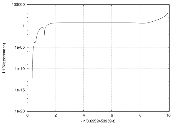
For our numerical test case here, we choose $a_{3}=0.7$ , $C_{2}=0.1$ and $E_{0}=0$ in Eqs. (17) as initial data parameters, corresponding to the “large inhomogeneity case” in [3] and to one of the simulations presented in [4]. The associated solution turns out to develop a singularity, and hence can be seen as an interesting test case for our code. The evolution of a spatial norm of the curvature invariant called Kretschmann scalar is shown in Fig. 2. All the results we show here were done without the automatic spatial adaption approach described in Section 2.4.1, because, in order to study convergence, it seems more useful to control and adapt the spatial resolution manually. The adaption norm, computed with respect to $E_{13}$ , was used only for estimating the aliasing error. The time integration was done with the adaptive $5$ th order embedded RK scheme with control parameters $\eta$ and $h_{\min}$ as discussed in Section 2.4.1. For these runs, we decided to use the “partial enforcement” scheme of the boundary conditions, explained in Section 3.1.3. All runs were done with double precision.

Refer to caption — Fig. 1: Evolution of curvature for the “large inhomogeneity case”

The constraints Eq. (16) are satisfied initially up to machine precision. However, due to numerical errors, those constraints typically become violated more and more with increasing evolution time. Let us define $\mathrm{Norm}^{(\textit{constr})}$ as the $L^{1}$ -norm of the sum of the absolute values of each of the six components of the left hand sides of Eqs. (16) at a given instant of time, all that divided by $\mathrm{tr}\,(\chi_{ab})$ , in order to factor out the observed collapse of the solution. $L^{p}$ -norms of functions on $\mathbb{S}^{3}$ are always evaluated here by means of their corresponding functions on $\mathbb{T}^{3}$ and the standard $L^{p}$ -norm on $\mathbb{T}^{3}$ . Another norm, which measures how well the numerical solution satisfies Einstein’s field equations, is

\mathrm{Norm}^{(\textit{einstein})}:=\left\|(\tilde{R}_{ij}-\lambda\tilde{g}_{ij})/\Omega(t)\right\|_{L^{1}(\mathbb{S}^{3})},

where the Ricci tensor $\tilde{R}_{ij}$ of the physical metric $\tilde{g}_{ij}$ is evaluated algebraically from the conformal Schouton tensor $L_{ij}$ and derivatives of the conformal factor $\Omega$ . The indices in this expression are defined with respect to the physical orthonormal frame given by $\tilde{e}_{i}=\Omega e_{i}$ . The norm is computed by summing over the $L^{1}$ -norms of each component.

Now, we will distinguish two phases of the evolution for these initial data, in which different aspects and effects are important: the early evolution close to $\mathcal{J}^{+}$ for $t$ between $0.0$ and $0.69$ , and the late evolution close to the singularity, which we find at $t\approx 0.69520493$ . In order to avoid confusions, we recall that the terms “early” and “late” are always understood with respect to the time coordinate $t$ , which, however, runs backwards with respect to the physical time.

At early times, it is achieved easily that the spatial discretization error is not significant, until some later time when small spatial structure starts to form more rapidly. One hint that this is true, as we do not show here, is that $\mathrm{Norm}^{(\textit{adapt})}$ is more or less constant over a long time period, and small. Another hint is that the behaviors of $\mathrm{Norm}^{(\textit{constr})}$ and $\mathrm{Norm}^{(\textit{einstein})}$ are not strongly influenced by the spatial resolution. See Fig. 2 and 4, where $N$ represents the number of spatial grid points, which is constant in this early regime. Indeed, the higher $N$ , the larger is the initial value $\mathrm{Norm}^{(\textit{constr})}$ due to higher round-off errors for computing spatial derivatives. This is not visible for $\mathrm{Norm}^{(\textit{einstein})}$ , since this quantity is defined purely algebraically in the unknowns. In Fig. 2, we see that $\mathrm{Norm}^{(\textit{constr})}$ grows less, the higher the time resolution is, i.e., in particular, the smaller the parameters $\eta$ and eventually also $h_{min}$ are. However, we always observe at least weak approximately exponential growth. In Fig. 4, we see a similar behavior for $\mathrm{Norm}^{(\textit{einstein})}$ . We do not show here that there is neither a particular growth of $\mathrm{Norm}^{(\textit{constr})}$ , nor of $\mathrm{Norm}^{(\textit{einstein})}$ , at the symmetry axes. Rather, the maximal growth takes place, where the curvature increases most strongly. This can be seen as a confirmation that our treatment of the coordinate singularities works well, cf. [3]. Note that there is an optimal time resolution, in the sense that, if we choose a higher resolution, the constraint error and $\mathrm{Norm}^{(\textit{einstein})}$ are actually increased caused by higher round-off errors. Although we do not show any plots, we want to mention, that we have experimented with “quad precision”. For the $1+1$ -code, this yields reasonable performance and has several consequences. First, the initial data for the constraint violations are decreased by many orders of magnitude, since those are determined primarily by the precision of the numerical number representation. By choosing appropriate resolutions, we find that the constraint violations and $\mathrm{Norm}^{(\textit{einstein})}$ can then be kept several orders of magnitude smaller than in the double precision case during the whole run. However, they always show exponential growth, which suggests that this is the typical behavior of the constraint propagation in our system of equations. Furthermore, quad precision allows us to work in a regime in which discretization errors are much larger than round-off errors, and hence it is easier to interpret convergence tests.

Fig. 4 shows the behavior of $\mathrm{Norm}^{(\textit{BC})}$ . The errors at the boundaries are small and stable, despite of some weak growth, which is expected in situations close to a singularity. In these tests, this error does not decrease for higher resolutions, which is a hint that round-off errors have a significant effect. With quad precision, we were able to confirm that the violations of the boundary conditions become smaller, consistent with increasing resolution.

Concerning the late evolution, the following is found. The following figures, Fig. 6 to Fig. 8, show a very small time neighborhood of the final time, where the runs were stopped and where the solution blows up. In the runs underlying these plots, we adapted the spatial resolution several times during the runs manually; the number $N$ in the figures is the final spatial resolution in each case. Each manual spatial adaption step is visible in the plots as a jump, because for different spatial resolutions, the numerical values of the norms slightly change. In all these runs, we choose $\eta=10^{-13}$ , and hence the time steps $h$ decrease so strongly that $h=h_{min}$ at that time when the runs were stopped. In this late time regime, the errors are dominated by spatial discretization errors, because the solution has the property that spatial structures shrink without bound. This can be seen by looking at the late time plot of the adaption norm in Fig. 6. It shows, how strongly the demand for spatial resolution grows with time, but also, that it is possible to gain control by increasing the resolution at least temporarily. However, the demand for spatial resolution increases very strongly with time, and it turns into a difficult numerical issue to keep track of that eventually. In Fig. 6, we demonstrate, how the choice of spatial resolution influences the propagation of the constraint violations, and that this quantity converges to a weakly exponentially growing for sufficiently high spatial resolutions. This is a promising result, and shows that the constraint propagation is more or less under control, as long as it is possible to increase the resolution in practice.

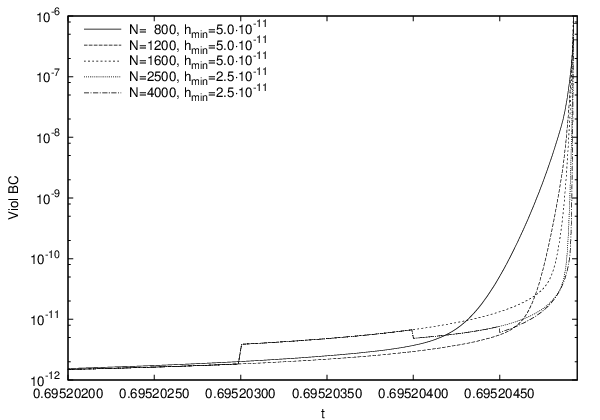
Fig. 8 shows the violations of the boundary conditions. They turn out to be very small and under control for sufficiently large resolutions. The higher the final spatial resolution is, the smaller these violations appear. Finally, in Fig. 8 we show $\mathrm{Norm}^{(\textit{einstein})}$ . We do not observe a very strong difference between the various resolutions; indeed, in order to make the differences visible at all, the time axis represents an even smaller time neighborhood now. It is unexpected that at very late times this norm is not necessarily smaller the higher the resolution is, and it has to be investigated whether this is a problem.

3.2.2 Comparison of a computation with the $2+1$ - and $1+1$ -code for a Gowdy symmetric solution

Next, we want to compare directly the numerical results obtained with the $2+1$ -code and the $1+1$ -code for a Gowdy symmetric solution of our equations. We restrict to a singularity free case, since we do not want to be spoiled by the lack of spatial resolution, in particular for the $2+1$ -code. The following initial data parameters are chosen: $a_{3}=0.93$ , $E_{0}=0$ and $C_{2}=0.5$ , which correspond to the “regular case” in [3]. The corresponding solution is smooth for all $0\leq t\leq 2$ and hence develops a smooth past conformal boundary at $t=2$ . Fig. 9 shows the evolution of the curvature invariant Kretschmann scalar. We show neither convergence plots, nor the error quantities before, since the situation is very similar to the early phase of the singular solution in the previous section. Instead, we report only on one run done with one fixed resolution: the size of the time step is $h=5\cdot 10^{-4}$ and the number of spatial points is $N=40$ for the $1+1$ -code and $N_{\chi}=41$ , $N_{\rho_{1}}=21$ for the $2+1$ -code. We use the non-adaptive $4$ th order RK time integrator, and the automatic spatial adaption has been switched off here as well.

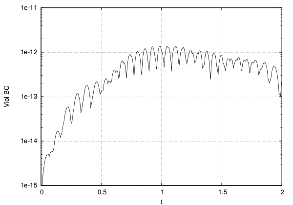
The run with the $1+1$ -code was done without enforcing the boundary conditions now, cf. Fig. 11. We see that this error stays very small and is stable. In order to illustrate, how well the results obtained with the $1+1$ - and the $2+1$ -code coincide, let us define the following norm

\mathrm{Norm}^{(\textit{diff})}:=\Bigl|(E_{11}^{(1+1)}|_{\chi=\pi})-(E_{11}^{(2+1)}|_{\chi=\pi,\,\rho_{1}=0})\Bigr|.

Consider Fig. 11 where this norm is plotted vs. time. We find very good agreement between the two codes. Some deviations can be expected, since in the $2+1$ -code, Gowdy symmetry is valid only approximately; see more comments in [3]. So far, we have made no effort to explain the oscillatory behavior in both figures, but we conjecture them to be caused by aliasing, since its amplitude becomes smaller, the higher the spatial resolution is. We have also compared more variables at other grid points and found similar results.

4 Summary and conclusions

The purpose of this paper is to introduce our numerical approach for the study of evolution equations with spatial $\mathbb{S}^{3}$ -topology. First, we have given details on a geometric point of view in order to find a natural discretization. Second, we have discussed issues related to the implementation and, third, analyzed test applications. By all this we have demonstrated the feasibility of this approach. Indeed, these techniques have been applied elsewhere, for instance in [3, 4, 5].

Although our main interest lies in the field of general relativity, we believe that the applicability of the method is more general. For the presentation of this paper, we made a couple of special choices which need to be overcome in order to use the method in more general situations. First, our analysis is based on $\mathrm{U(1)}$ -symmetry so far. We believe that it is straight forward to generalize in principle. Furthermore, we decided to formulate the equations in terms of smooth global frames on $\mathbb{S}^{3}$ . This had the consequence that only singular terms of special type are present, and with this knowledge, we were able to work out the Fourier series of the formally singular terms explicitly in Section 2.2. However, in general, as soon as we have a-priori knowledge about the structure of the formally singular terms in the equations, and if their type is not completely different than ours, a similar regularization is possible. Hence, from this point of view, one should be able to modify our method to cases, where other kinds of frames or spatial coordinates are used. In our application, we made a special choice of coordinate gauge and frame transport. This implied that, in particular, the matrix $(T^{\mathchoice{\makebox[4.33765pt][c]{$\displaystyle$}}{\makebox[4.33765pt][c]{$\textstyle$}}{\makebox[2.59009pt][c]{$\scriptstyle$}}{\makebox[1.85005pt][c]{$\scriptscriptstyle$}}{a^{\prime}}}_{{a}\mathchoice{\makebox[6.18513pt][c]{$\displaystyle$}}{\makebox[6.18513pt][c]{$\textstyle$}}{\makebox[4.05258pt][c]{$\scriptstyle$}}{\makebox[3.31255pt][c]{$\scriptscriptstyle$}}})$ is constant in time. If the original evolution equations imply a well-posed initial value problem, then, in this gauge, also the evolution equations for Gowdy symmetry reduced to $1+1$ dimensions have this property. For other gauges, however, this might not be the case. A further issue turns up when the frame transport does not keep the orthonormal frame boundary adapted in the sense of Section 3.1.3. Then a different boundary treatment than ours might become necessary. As a last point of this certainly incomplete list, we mention that we have not made experiments with other time integrators yet. Of particular interest might be implicit schemes, for instance, to treat parabolic evolution equations.

We believe that our current numerical infrastructure has not yet been pushed to its limits, but is also not yet really optimized for high spatial resolutions. For instance, we still do not use FFT but only the partial summation scheme. Also it may be true, that there is a more optimal trade-off between accuracy and efficiency for other time integrators than the Runge Kutta schemes of our choice; comments on this can be found in [6]. Furthermore, it might make sense to think about parallelization of the code. This should be straight forward with some publicly available FFT libraries, for instance [17]. We expect, that the $1+1$ -code, in its current form, is limited to a few thousand spatial grid points. We want to stress that this turned out to be sufficient in our runs with $\mathbb{T}^{3}$ -topology in [3]. There, we were able to reproduce “spiky features” numerically. Hence, we are optimistic that also such difficult phenomena can be studied with our numerical infrastructure in $1+1$ dimensions. Dependent on the kind of the application, one may nevertheless doubt, if spectral methods are suitable at all. In general, it is fair to say that, although these methods are highly accurate for lower resolutions, they might be too inefficient for high resolutions. Thus it makes sense, to also investigate into other methods, for instance finite differencing methods, maybe with multipatch [38, 11, 27], in order to make systematic comparison studies. Further automatic local spatial adaption, usually called adaptive mesh refinement, would be desirable; for instance cosmological solutions with spikes have been investigated with such techniques in [20], however not for $\mathbb{S}^{3}$ -topology.

In summary, due to the results of the tests here and in [3, 4, 5], we believe that our numerical approach has promising potentials, which have not been fully exhausted yet, for many kinds of applications with spatial $\mathbb{S}^{3}$ -topology and beyond. For instance, we find it particularly appealing that our infrastructure can be used directly also for problems with spatial $\mathbb{T}^{3}$ -topology and, at least for Gowdy symmetry, with $\mathbb{S}^{1}\times\mathbb{S}^{2}$ -topology [5]. For the applications, which we have in mind, future research will show, how much the method must be modified, or whether completely new approaches will become necessary, in order to deal with probably much more severe phenomena than those present in the classes of solutions considered so far.

Acknowledgments

This work was supported in part by the Göran Gustafsson Foundation, the Partner Group of the Max Planck Institute for Gravitational Physics in FaMAF, Córdoba, Argentina, and by the Agence Nationale de la Recherche (ANR) through the Grant 06-2-134423 entitled Mathematical Methods in General Relativity (MATH-GR) at the Laboratoire J.-L. Lions (Université Pierre et Marie Curie). We would like to thank in particular Jörg Frauendiener, Helmut Friedrich and David Garfinkle for discussions and comments, and the relativity group at FaMAF in Córdoba also for their hospitality.

References

[1] L. Andersson and G.J. Galloway. dS/CFT and spacetime topology. Adv. Theor. Math. Phys., 6:307–327, 2002, hep-th/0202161.
[2] R. A. Bartnik and A. H. Norton. Einstein equations in the null quasi-spherical gauge. III: Numerical algorithms. preprint, 1999, gr-qc/9904045.
[3] F. Beyer. Asymptotics and singularities in cosmological models with positive cosmological constant. PhD thesis, Max Planck Institute for Gravitational Physics, Sep. 2007, gr-qc/0710.4297.
[4] F. Beyer. Investigations of solutions of Einstein’s field equations close to $\lambda$ -Taub-NUT. Class. Quant. Grav., 25:235005, 2008, arXiv:0804.4224 [gr-qc].
[5] F. Beyer. Investigations of the instability of Nariai asymptotics within the Gowdy class. preprint, 2009, arXiv:0902.2532 [gr-qc].
[6] J.P. Boyd. Chebyshev and Fourier Spectral Methods. Dover Publications, Inc., 2nd edition, 2001.
[7] C. Canuto, M.Y. Hussaini, A. Quarteroni, and T.A. Zang. Spectral Methods in Fluid Dynamics. Springer, 1988.
[8] M.W. Choptuik, E.W. Hirschmann, S.L. Liebling, and F. Pretorius. An axisymmetric gravitational collapse code. Class. Quant. Grav., 20:1857–1878, 2003, gr-qc/0301006.
[9] P. Chruściel, J. Isenberg, and V. Moncrief. Strong cosmic censorship in polarized Gowdy space-times. Class. Quant. Grav., 7:1671–1680, 1990.
[10] J.W. Cooley and J.W. Tukey. An algorithm for the machine calculation of complex Fourier series. Math. Comput., 19:297–301, 1965.
[11] P. Diener, E.N. Dorband, E. Schnetter, and M. Tiglio. New, efficient, and accurate high order derivative and dissipation operators satisfying summation by parts, and applications in three-dimensional multi-block evolutions. J. Sci. Comput., 32:109–145, 2007, gr-qc/0512001.
[12] M.D. Duez, F. Foucart, L.E. Kidder, H.P. Pfeiffer, M.A. Scheel, and S.A. Teukolsky. Evolving black hole-neutron star binaries in general relativity using pseudospectral and finite difference methods. Phys. Rev. D, 78(10):104015, 2008.
[13] H. Friedrich. Existence and structure of past asymptotically simple solutions of Einstein’s field equations with positive cosmological constant. J. Geom. Phys., 3(1):101–117, 1986.
[14] H. Friedrich. Einstein equations and conformal structure: Existence of anti-De Sitter-type spacetimes. J. Geom. Phys., 17:125–184, 1995.
[15] H. Friedrich. The Conformal Structure of Spacetime: Geometry, Analysis, Numerics, chapter ”Conformal Einstein Evolution”. Lecture Notes in Physics. Springer, 2002.
[16] H. Friedrich and G. Nagy. The initial boundary value problem for Einstein’s vacuum field equations. Commun. Math. Phys., 201:619–655, 1999.
[17] M. Frigo and S.G. Johnson. FFTW Library, http://www.fftw.org/.
[18] D. Garfinkle. Numerical simulations of Gowdy spacetimes on $S^{2}\times S^{1}\times R$ . Phys. Rev. D, 60(10):104010, Oct. 1999, gr-qc/9906019.
[19] D. Garfinkle and G.C. Duncan. Numerical evolution of Brill waves. Phys. Rev. D, 63:044011, 2001, gr-qc/0006073.
[20] D. Garfinkle, W.C. Lim, F. Pretorius, and P.J. Steinhardt. Evolution to a smooth universe in an ekpyrotic contracting phase with $w>1$ . Phys. Rev., D78:083537, 2008, arXiv:0808.0542 [gr-qc].
[21] R.H. Gowdy. Vacuum space-times with two parameter spacelike isometry groups and compact invariant hypersurfaces: Topologies and boundary conditions. Ann. Phys., 83:203–241, 1974.
[22] S.W. Hawking and G.F.R. Ellis. The large scale structure of space-time. Cambridge University Press, 1973.
[23] J. Hennig and M. Ansorg. A Fully Pseudospectral Scheme for Solving Singular Hyperbolic Equations. preprint, 2008, arXiv:0801.1455 [gr-qc].
[24] Intel. Intel Fortran Compiler, http://www.intel.com/support/performancetools/.
[25] J. Isenberg and V. Moncrief. Asymptotic behavior of the gravitational field and the nature of singularities in Gowdy space-times. Ann. Phys., 199:84–122, 1990.
[26] F. John. Partial Differential equations. Springer, 4th edition, 1982.
[27] L. Lehner, O. Reula, and M. Tiglio. Multi-block simulations in general relativity: high order discretizations, numerical stability, and applications. Class. Quant. Grav., 22:5283–5322, 2005, gr-qc/0507004.
[28] A. Majda. Compressible Fluid Flow and Systems of Conservation Laws in several space dimensions. Springer, 1984.
[29] B. O’Neill. Semi-Riemannian Geometry with Applications to Relativity. Academic Press, Inc, 1983.
[30] R. Penrose. Asymptotic properties of fields and space-time. PRL, 10:66–68, 1963.
[31] R. Penrose. Singularities and time-asymmetry. In S.W. Hawking and W. Israel, editors, General Relativity – An Einstein Centenary Survey. Cambridge University Press, 1979.
[32] H.P. Pfeiffer, L.E. Kidder, M.A. Scheel, and S.A. Teukolsky. A multidomain spectral method for solving elliptic equations. Comput. Phys. Commun., 152:253–273, 2003, gr-qc/0202096.
[33] W.H. Press, S.A. Teukolsky, W.T. Vetterlin, and B.P. Flannery. Numerical Recipes in C. Cambridge University Press, 2nd edition, 1999.
[34] O. Rinne. Axisymmetric numerical relativity. PhD thesis, University of Cambridge, 2005, gr-qc/0601064.
[35] M. A. Scheel, H. P. Pfeiffer, L. Lindblom, L. E. Kidder, O. Rinne, and S. A. Teukolsky. Solving Einstein’s equations with dual coordinate frames. Phys. Rev. D, 74:104006, 2006, gr-qc/0607056.
[36] F. Ståhl. Fuchsian analysis of $S^{2}\times S^{1}$ and $S^{3}$ Gowdy spacetimes. Class. Quant. Grav., 19:4483–4504, 2002, gr-qc/0109011.
[37] M. Sugiura. Unitary Representations and Harmonic Analysis. North-Holland, Kodansha, 2nd edition, 1990.
[38] J. Thornburg. Black-hole excision with multiple grid patches. Class. Quant. Grav., 21:3665–3691, 2004.
[39] P. Topping. Lectures on the Ricci Flow. Cambridge University Press, 2006.
[40] J. Wainwright and G.F.R. Ellis. Dynamical Systems in Cosmology. Cambridge University Press, 1997.

A spectral solver for evolution problems with spatial 𝕊3\mathbb{S}^{3}-topology