Signatures of a hidden cosmic microwave background
Abstract
If there is a hidden photon – i.e. a light abelian gauge boson in the hidden sector – its kinetic mixing with the standard photon can produce a hidden cosmic microwave background (hCMB). For meV masses, resonant oscillations happen after nucleosynthesis (BBN) but before CMB decoupling, increasing the effective number of neutrinos () but also the baryon to photon ratio at decoupling. The current agreement between BBN and CMB data provides new constraints on the kinetic mixing. However, if one includes Lyman- data, is preferred. It is tempting to interpret this effect in terms of the hCMB. Interestingly, the required parameters will be tested in the near future by laboratory experiments.
pacs
14.70.Pw, 98.80.CqMost embeddings of the standard model into a more unified theory, in particular the ones based on supergravity or superstrings, predict the existence of a hidden sector whose inhabitants have only very weak interactions with the standard model. The gauge interactions in the hidden sector generically involve U(1) factors. Usually, it is assumed that the corresponding gauge bosons are very heavy, in order to avoid observational constraints. However, in realistic string compactifications, one of these hidden photons may indeed be light, with a mass in the sub-eV range, arising from a Higgs or Stückelberg mechanism. In this case, the dominant interaction with the visible sector photon will be through gauge kinetic mixing [2], i.e. the system can be parametrized by the low-energy effective Lagrangian,
| (1) | |||||
where and are the photon () and hidden photon () field strengths. The dimensionless mixing parameter can be generated at an arbitrarily high energy scale and does not suffer from any kind of mass suppression from the messenger particles communicating between the visible and the hidden sector. This makes it an extremely powerful probe of high scale physics. Typical predicted values for in realistic string compactifications range between and [3].
The most prominent implication of the kinetic mixing term is that photons are no longer massless propagation modes. Similar to neutrino mixing the propagation and the interaction eigenstates are misaligned. The kinetic mixing term can be removed by changing the basis , where , . Since and differ only by a typically unobservable charge renormalization we will drop the subscript from now on. In the basis the kinetic term is diagonal but kinetic mixing provides an off-diagonal term in the mass-squared matrix,
| (2) |
As a result one expects vacuum photon-sterile oscillations [4] as in the case of .
In this letter, we examine the implications of this simple scenario for late cosmology.
We focus on the meV mass range where a thermal population of hidden photons can be created through
resonant oscillations after BBN but before CMB decoupling.
This ‘hidden CMB’ (hCMB) will contribute to the effective number of additional neutrinos at decoupling and,
since some photons will disappear, will increase the baryon to photon ratio with respect to the BBN value.
Moreover, we will argue that possible distortions of the thermal nature of the CMB spectrum are very small
in the parameter range allowed by other constraints.
Effects of a post BBN hCMB production.- Let us assume that at the time of BBN there is no hidden photon thermal bath present. For the case where kinetic mixing is the only interaction with standard model particles, this will be justified later. Additional light particles charged under the hidden U(1)h would appear as minicharged particles (MCPs) which could mediate the formation of a hCMB before BBN. Given the existent constraints on the number of additional neutrinos at BBN and on MCPs [5] we will not discuss this possibility here and focus instead on the case when there is only a hidden photon.
The oscillation of photons into hidden-sector photons decreases the photon number and energy density () leaving the total energy unchanged. The key parameter will be the fraction of that is converted into hidden photons, .
We will see that inelastic processes are effective after hCMB decoupling. Therefore the remaining photons will regain a black body distribution, albeit, due to the energy loss, at a lower temperature,
| (3) |
Since neutrinos remain unchanged during the hCMB formation, the ratio of neutrino and photon temperatures will also increase. The invisible energy density (in radiation) at decoupling can be estimated using CMB anisotropies and is often quoted as the effective number of ‘standard’ neutrinos, by normalizing it with . In our case,
| (4) |
is the sum of neutrino and hidden photon contributions.
Strong limits on at decoupling arise from global fits of CMB anisotropies alone [6] or combined with large scale structure data [7]. Inclusion of Lyman- data favors values [8], although this might well be due to systematics [9]. A recent analysis of WMAP5 plus other CMB anisotropy probes, large scale structure (no Ly-) and supernovae data provides [10]
| (5) |
which, using the standard, , turns (5) into
| (6) |
As a conservative example of the inclusion of Ly- data we propose [9], suggesting . It is worth noting however that values as high as can be found also in the literature [8].
Since is proportional to , the baryon to photon ratio (which would otherwise remain constant) is also modified according to
| (7) |
Indeed the value for inferred from the abundances of the light elements produced at BBN and the one obtained by measuring temperature fluctuations in the CMB [10] agree within their error bars,
| (8) | |||
| (9) |
which allows us to set the bound .
Photon oscillations in the early universe plasma.- The formalism to study the dynamics of a thermal bath of particles that undergo ‘flavor’ oscillations among the different species was developed some time ago [11, 12], for a textbook treatment see [13].
The state of an ensemble of and is described by a 2-by-2 density matrix,
| (10) |
where has the Pauli matrices as components and is a ‘flavor polarization vector’ carrying all the information of the ensemble. The modulus gives the degree of coherence, corresponding to a pure () state, while to a completely incoherent state, which of course defines the state of ‘flavor equilibrium’. The transverse components contain the quantum correlations.
The time evolution of the ensemble is given by a precession of (flavor oscillations) and a shrinking of its transverse component (decoherence due to absorption and scattering), according to Stodolsky’s formula [12]
| (11) |
Here is the ‘flavor magnetic field’ given by
| (12) |
where is the energy and we have included the refraction properties of the medium (basically an electron plasma) as a photon ‘effective mass’, given by the plasma frequency with the fine-structure constant, and the electron mass and density.
The damping factor equals half the collision rate of photons [12], here dominated by Thomson scattering, .
Before dealing with the details of the calculation, we will try to gain some intuition about the main points of the cosmology of the system. For temperatures below keV, electrons and positrons have annihilated leaving an electron relic density which balances the charge of protons, namely . Using the BBN central value (8), we find
| (13) |
As the universe expands, the density decreases and so do the plasma mass and absorption rate. The ratio is, however, independent of and very small, . Therefore the damping term in (11) is typically smaller than the precession rate , the only possible exception being the resonant case to be discussed later. In this situation we can use the precession-averaged in (11), which then turns into [13]. Under these conditions a significant hCMB will form if the rate
| (14) |
exceeds the expansion rate of the universe, given by the Hubble parameter eV.

Isocontours of have been plotted in Fig. 1, showing the possible history of the hCMB formation for different values of and . During its evolution, the universe moves on a horizontal line of fixed from high temperature (right) to low temperatures (left). We can clearly distinguish three different regimes separated in time by a resonant peak occurring at , the temperature at which has decreased enough to match exactly .
a) In an early stage, for , is so large that the hidden photon is comparatively massless; photons are very close to being both interaction and propagation eigenstates and oscillations are strongly suppressed by the effective mixing angle given by
| (15) |
This is in contrast to the usual cosmology of exotic particles. Light hidden photons are completely decoupled for high enough temperatures (as long as their only relevant coupling is the kinetic mixing). This justifies our earlier claim and allows us to set the initial conditions for the system to , i.e. a pure photon bath without hidden photons. As the temperature approaches , increases and can even be enhanced compared to . Hidden photons will be effectively produced when crossing the line in Fig. 1.
b) In a small region around , the production can be effective even for very small . Unfortunately, the precession average is not justified because typically . Below we provide details on the calculation in this regime.
c) For , the averaging procedure is again justified.
In this regime, and we recover the well known vacuum case.
The evolution will again freeze out after crossing the line
in Fig. 1.
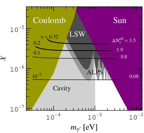
Resonant production.- ¿From Fig. 1 it is clear that for (larger values are excluded by laboratory experiments, see Fig. 2) production is effective only in the resonant regime. Therefore, we need an approximation that is valid in the vicinity of the resonance. Moreover, since the resonance happens only for a short period of time, the simple criterion is not sufficient to ensure that a sizable hCMB is produced. Accordingly we have to calculate the integrated production.
In the vicinity of the resonance, the oscillation frequency is minimal () and indeed typically much smaller than the damping factor . The evolution of in a general ‘strong damping’ regime was studied in [12] where it was found that the flavor relaxation rate is given by
| (16) |
with and . The strong damping condition reads simply . In the interesting region this is typically fulfilled because . At the low energy end of the spectrum we will typically violate the strong damping regime, but this region contributes comparatively little to the energy density.
The physical meaning of (16) is clear regarding (11). Since damps , will rapidly become attached to the axis (regardless of the initial value). Note that, for , is a stationary solution of (11) for which the production rate would vanish. Now let us switch on a small . The precession caused by tries to move away from the -axis. However, any transverse component is immediately damped away again because . While the precession keeps constant, it is decreased by the damping. Therefore, while the direction of will remain roughly constant, its modulus will slowly decrease in time and we approach ‘flavor equilbrium’ at a rate (16).
Integrating Eqs. (11), (16) over time we can calculate the transition probability,
| (17) |
where we have used a parametrisation in terms of the temperature instead of time. Since the relevant part of the integral comes from the vicinity of the resonance, we expand the denominator of around up to the relevant quadratic term. Expressed in terms of , and using finally , the integral is
| (18) | |||
where we have evaluated the braced combination at (since it does not depend on ) and used .
Our main result, namely the fraction of the energy stored in the hCMB, is obtained by integrating the probability over the Boltzmann distribution,
| (19) |
To be conservative we shall cut off the integral at small frequencies where the strong damping approximation breaks down, , corresponding to keV. If is large, this can affect a sizable part of the spectrum. Otherwise, we obtain an analytic expression by expanding (17),
| (20) |
During this epoch, double Compton scattering is active,
since is
typically (for meV). Therefore the remaining photons will
regain a black body spectrum after the resonant production.
Discussion and conclusions.- In the region , the fraction of photons converted into hidden photons depends only very weakly on the mass (cf. Eq. (20) and Fig. 2). For , the resonant production would be sufficiently strong to convert roughly half the photon energy into hidden photons. This would clearly be in contradiction with cosmological observations: even the conversion of a small part of the photon energy into hidden photons may leave observable traces in the effective number of relativistic species and in the baryon to photon ratio . Using , from the upper limit on in Eq. (5), or the slightly weaker constraint , from the upper limit on in Eq. (8), one obtains an upper bound , in the mass range (cf. Fig. 2). In the mass range , this improves upon the previously established upper bounds on – from searches for deviations from the Coulomb law and from light-shining-through-walls (LSW) experiments – by a factor of up to (cf. Fig. 2).
As mentioned earlier, inclusion of Lyman- data seems to favor higher values of [8, 9]. It is tempting to interpret this in terms of an hCMB (for an alternative explanation see [20]). Fortunately, the parameter region corresponding to the required energy fraction, , can be explored in the near future by pure laboratory experiment, notably by LSW experiments [16] or an experiment exploiting microwave cavities [18] (cf. Fig. 2). Furthermore, the hidden photon CMB itself could be tested by an experiment like ADMX [21] in which hidden photons entering a cavity can be reconverted into detectable ordinary photons.
References
- [2] B. Holdom, Phys. Lett. B 166, 196 (1986); R. Foot, and X. G. He, Phys. Lett. B 267, 509 (1991).
- [3] K. R. Dienes et al., Nucl. Phys. B 492, 104 (1997); S. A. Abel and B. W. Schofield, Nucl. Phys. B 685, 150 (2004); S. A. Abel et al., hep-ph/0608248; 0803.1449 [hep-ph].
- [4] L. B. Okun, Sov. Phys. JETP 56, 502 (1982).
- [5] S. Davidson, S. Hannestad and G. Raffelt, JHEP 0005, 003 (2000).
- [6] K. Ichikawa et al., 0803.0889 [astro-ph]; J. Dunkley et al. [WMAP], 0803.0586 [astro-ph].
- [7] G. Mangano et al., JCAP 0703, 006 (2007); K. Ichikawa, M. Kawasaki and F. Takahashi, JCAP 0705, 007 (2007); E. Komatsu et al. [WMAP], 0803.0547 [astro-ph].
- [8] U. Seljak et al., JCAP 0610, 014 (2006); M. Cirelli and A. Strumia, JCAP 0612, 013 (2006).
- [9] J. Hamann et al., JCAP 0708, 021 (2007).
- [10] V. Simha and G. Steigman, 0803.3465 [astro-ph].
- [11] R. A. Harris and L. Stodolsky, Phys. Lett. B 116, 464 (1982).
- [12] L. Stodolsky, Phys. Rev. D 36, 2273 (1987).
- [13] G. G. Raffelt, “Stars As Laboratories For Fundamental Physics” Chicago, USA: Univ. Pr. (1996) 664 p
- [14] D. F. Bartlett and S. Loegl, Phys. Rev. Lett. 61, 2285 (1988); E. R. Williams, J. E. Faller and H. A. Hill, Phys. Rev. Lett. 26, 721 (1971).
- [15] J. Redondo, 0801.1527 [hep-ph].
- [16] M. Ahlers et al., 0711.4991 [hep-ph], and refs. therein.
- [17] See http://alps.desy.de/e55 .
- [18] J. Jaeckel and A. Ringwald, Phys. Lett. B 659, 509 (2008).
- [19] S. Gninenko and J. Redondo, 0804.3736 [hep-ex].
- [20] K. Ichikawa et al., JCAP 0705, 008 (2007).
- [21] S. Asztalos et al., Phys. Rev. D 64, 092003 (2001).