Coupling-geometry-induced temperature scales in the conductance of Luttinger liquid wires
Abstract
We study electronic transport through a one-dimensional, finite-length quantum wire of correlated electrons (Luttinger liquid) coupled at arbitrary position via tunnel barriers to two semi-infinite, one-dimensional as well as stripe-like (two-dimensional) leads, thereby bringing theory closer towards systems resembling setups realized in experiments. In particular, we compute the temperature dependence of the linear conductance of a system without bulk impurities. The appearance of new temperature scales introduced by the lengths of overhanging parts of the leads and the wire implies a which is much more complex than the power-law behavior described so far for end-coupled wires. Depending on the precise setup the wide temperature regime of power-law scaling found in the end-coupled case is broken up in up to five fairly narrow regimes interrupted by extended crossover regions. Our results can be used to optimize the experimental setups designed for a verification of Luttinger liquid power-law scaling.
pacs
71.10.Pm, 73.63.Nm, 71.10.-w1 Introduction
Theoretically, it is well established that the low-energy physics of a wide class of one-dimensional (1d) metallic electron systems (quantum wires) with two-particle interaction is described by the Luttinger Liquid (LL) phenomenology [1]. One of the characterizing properties of LL physics is the power-law scaling of a variety of physical observables as function of external parameters. For spin-rotationally invariant and spinless systems the corresponding exponents can all be expressed in terms of a single parameter, the LL-parameter . On the experimental side the situation is less clear. Much effort has been put into measurements aiming at a verification of LL behavior by observing the predicted power-law scaling. However, in many of those experiments sources for the observed behavior other than LL physics cannot be ruled out in a completely satisfying way [2].
The gap between the status of theory and experiment is partly related to an insufficient theoretical modeling of the experimentally available setups. In many experiments on quantum wires realized e.g. by single wall carbon nanotubes or semiconductor heterostructures, the temperature dependence of the linear conductance was measured [3]. A typical experimental system in which the finite-length LL wire is coupled via tunnel barriers to two quasi two-dimensional, stripe-like (Fermi liquid) leads is sketched in figure 1. In the preparation the precise position of the contact regions and its width, as well as the quality of the contacts is still difficult to control. In contrast to the experimental geometry the theoretical description is mostly done by considering end-contacted wires, in which the lead electrons tunnel into the end of the wire and the leads terminate at the contacts. Here we partly bridge the gap between the simplicity of the theoretical modeling and the complexity of the experimental setup by considering a microscopic model of a quantum wire with 1d as well as stripe-like (two-dimensional) leads, which arbitrarily couple to the wire. Undoubtedly, in order to achieve direct comparison to experimental data true ab-initio simulations of the specific experimental setup would be desirable. Yet, the available ab-initio methods do not capture LL physics and thus cannot be used in the present context. Therefore, microscopic modeling is the method of choice to extend the LL physics originally derived within effective field-theories. We show that the length scales set by the overhanging parts of the leads and the wire introduce new energy scales, which strongly affect the temperature dependence of the conductance. The curves become much more complex than the ones obtained from the simplified modeling.

Throughout this paper we consider the case of spinless fermions. We expect that our results—with the appropriate changes [2] in the equations relating scaling exponents to the LL parameter —directly carry over to the case of spin- electrons if the two-particle interaction is long-ranged (unscreened) in real space (that is, if the term of the g-ology classification [4] can be neglected) and spin-rotationally invariant. This is generally assumed to be the case in single wall carbon nanotubes [5]. For semiconductor heterostructures the range of the interaction can strongly depend on the screening properties of the surrounding environment (free carriers). In the presence of a sizable backscattering component () the asymptotic low-energy regime is usually reached via a complex crossover behavior [6, 7, 8]. We expect the same to hold for the more realistic setups studied here, which would render the behavior of even more complex (and less “universal”) than described in the present work.
The most elementary understanding of the temperature dependence of the linear conductance of a LL wire can be gained using Fermi’s Golden Rule like arguments. The local single-particle spectral function of a translationally invariant, infinite LL scales as , with measured relative to the chemical potential and [2]. For a semi-infinite LL and , with being the distance from the boundary and denoting the Fermi velocity, the power-law scaling of the now -dependent spectral weight is instead given by the boundary exponent [9, 10]. Beyond the energy scale the bulk exponent is recovered. Fermis Golden Rule then predicts, for tunneling into the bulk of a LL while tunneling into the end leads to . The LL parameter (for repulsive interactions; in the noninteracting case) is model dependent [1, 2]. Only for a few cases (for an example see below) its exact dependence on the model parameters such as the strength of the two-particle interaction and the filling of the band is known analytically. For small interactions parameterized by the amplitude , generically goes as with the model and parameter dependent scale . From this Taylor expansion one can infer that is linear in and for small interactions dominates over which is quadratic.
In experimental setups the particles leave the LL wire at a second contact. To obtain the conductance of this type of system one is tempted to simply take the inverse of the sum of the two resistances resulting from the tunnel barriers. In the presence of inelastic scattering processes this is certainly correct. In the absence of such processes, an approximation used in the present paper, it is however less clear if this leads to the correct result for the conductance. In [11] and [12] it was shown using scattering theory that for low-transmittance contacts and at temperatures sufficiently larger than the scale , with the Fermi velocity and the length of the interacting wire, adding the two resistances and taking the invers gives the correct result. We note in passing that this can not be extended to the case of more than two impurities [12].
The Fermi Golden Rule like considerations on the conductance of a LL wire usually do not take the geometry of the reservoirs into account explicitely but only use their Fermi liquid properties. For the case of end-contacted wires the above results were confirmed within a microscopic modeling of the semi-infinite leads (1d noninteracting tight-binding chain) and the wire (1d tight-binding chain of spinless fermions with nearest-neighbor interaction) [11, 12]. The linear conductance shows power-law scaling for temperatures , with the number of lattice sites in the interacting wire and the bandwidth. Other approaches to include the end-contacted leads into the model are based on the so-called local Luttinger liquid picture [13] and on the concept of radiative boundary conditions [14], where the wire is modeled by an effective field-theory (bosonization) [2].
We here extend the functional renormalization group (fRG) approach used to study the linear response transport [11] as well as the finite bias steady-state nonequilibrium transport [15] through an end-contacted wire (described by a microscopic model) to investigate the role of the contacts and the leads more thoroughly. The reservoirs are modeled as two-dimensional tight-binding stripes of variable width (including the case of 1d leads) and contacted to the 1d interacting wire at arbitrary positions. This generically leads to overhanging parts of the wire as well as of the leads (see figure 1). We show that they set new energy scales and the temperature range of power-law scaling of , , breaks up into up to five different regimes of variable size. This leads to a temperature dependence of which is much richer than the simple scaling , which for sufficiently long wires, holds over several decades in within the simplified modeling described above. Our results show that it is difficult to find clear evidence for LL behavior of in the generically used setups.
To fully cover all relevant temperature regimes and treat systems of experimental length, i. e. in the micrometer range, we have developed an algorithm which allows us to compute the conductance for systems of up to lattice sites. Including the stripe-like leads requires a substantial extension of the order algorithm developed for 1d leads [16].
The rest of the paper is organized as follows. In section 2 the microscopic model used to describe the quantum wire and the leads is introduced. In section 3 and the appendix it is shown in detail, how to calculate the conductance through the system using scattering theory. Section 4 is a short survey of the fRG method and the generalizations necessary to include stripe-like leads are described. In section 5 our results for the temperature dependence of the conductance are presented and discussed. We conclude with a summary in section 6.
2 The Microscopic Model
We consider spinless fermions on a finite 1d lattice with nearest-neighbor hopping and nearest-neighbor two-body interaction , coupled to two semi-infinite, stripe-like, and noninteracting tight-binding leads. For simplicity all lattice constants are assumed to be equal and chosen to be unity. The system is sketched in figure 2. The Hamiltonian of the site quantum wire reads ()
with
| (1) |
where denotes the fermionic annihilation (creation) operator in Wannier states at site . We here consider the case of half-filling of the leads as well as of the wire. To assure the latter the density operator in the last line of (1) is shifted by . We expect similar results to hold away from half-filling.
The leads are assumed to be noninteracting
where stands for (left) and (right) and the symbol denotes the set of lattice points of lead . The extensions of the leads in the -direction given by are allowed to differ. The hopping matrix elements are assumed to connect nearest neighbors only.
The 1d wire and the stripe-like leads are coupled via hopping terms, described by
| (2) |
The matrix elements will be specified later.
The full Hamiltonian of the system reads
| (3) |
The model for an infinite isolated wire with interaction between all sites can be solved exactly using the Bethe ansatz [17]. The system is a LL for all fillings and interactions except for half-filling at , where a charge density wave forms () or phase separation occurs (). From the Bethe ansatz solution, the LL parameter can be computed and reads for half filling and [18]
| (4) |

3 Single particle scattering
3.1 General relations
The fRG procedure in the approximation scheme described in section 4 yields a frequency independent self-energy of the interacting wire at the end of the fRG flow. This can be interpreted as a single-particle (scattering) potential and incorporated into a renormalized single-particle Hamiltonian. As described in detail in [11] for end-coupled wires with 1d leads one can compute the conductance from single-particle scattering theory [19] using a generalized Landauer-Büttiker approach [20].
We therefore consider the single-particle Hamiltonian
| (5) |
where is the effective single-particle Hamiltonian for the wire at the end of the fRG flow (which includes the generated scattering potential) and the ’s are single-particle versions of the terms introduced in the last section. For the states in the single-particle Hilbert space we use standard Dirac notation. In the scattering problem to be solved, the first three terms of are considered to be the unperturbed part , while the couplings to the leads are considered as the perturbation . We closely follow the steps for the corresponding scattering problem with end-contacted, 1d leads [11].
The main difference of working with higher dimensional leads is the occurrence of transverse scattering channels. The orthonormal single-particle eigenstates of the isolated semi-infinite leads are standing waves with the wavenumber in the -direction and labeling the transverse modes
The corresponding eigenenergies are
| (6) | |||||
with the nearest-neighbor hopping matrix elements and .
We now consider the scattering of a particle from the left to the right lead (or vice versa) coupled via to the wire. The outgoing scattering states follow from the Lippmann-Schwinger equation [21]
| (7) |
where is the resolvent of the full single-particle Hamiltonian.
If we define as the “complement” of this yields
| (8) |
Using with we obtain
Only elastic scattering occurs with . This is enforced by the free resolvent matrix elements . It is easier to see this in a mixed representation, local in the -direction and using the transverse channel number as the additional quantum number
| (9) | |||||
The second equality holds for larger than the involved in the coupling of the lead and the quantum wire. To derive this relation we used the result for the resolvent of a semi-infinite 1d chain () with nearest-neighbor hopping
| (10) | |||||
where the second line holds for . For the wavenumber is the solution of and the velocity is given by . In [11] only the result for was presented. For the resolvent matrix element decays exponentially with the distance and are thus “closed” channels in (9). This happens if , and is determined by energy conservation . The velocity in (9) is given by . The prefactor of the outgoing plane wave in (9) gives the transmission probability for the scattering
| (11) | |||||
Taking the sum over compatible with and over the values of the corresponding “open” channels we define [20]
| (12) |
The unitarity of the -matrix guarantees . This quantity determines the conductance in the generalized Landauer-Büttiker formula [20]
| (13) |
where denotes the Fermi function and is the unit of the quantized conductance. Note that for our interacting problem the flowing self-energy and thus as well as the effective transmission probability become and dependent (for details, see below).
The Landauer-Büttiker formula (13) holds in the abscence of inelastic processes due to the two-particle interaction (that is for vanishing imaginary part of the self-energy) [19]. Such processes do not appear in our approximate treatment of the interaction and using (13) does thus not present an additional approximation.
For the calculation of the transmission probability one has to compute the matrix elements of the full resolvent. This can be reduced to the inversion of a -matrix, using Feshbach projection [11]
| (14) | |||||
where and are projection operators. Here we use as the projection operator onto the wire and the one on the leads.
The special geometry (mimicking a generic experimental setup) used in section 5 is shown in figure 3. Each site of the wire lying on top of a site of the lead (as shown in the figure) is coupled to this site via a hopping term . The length scales appearing in the system are also defined in the figure. Note that the overall length .

The projected inverse Green function takes the form shown in figure 17 of the appendix. We need the tridiagonal elements of this Green function to calculate the right-hand side of the flow equations (16) and (17), see section 4. An algorithm to compute these elements is presented in the appendix. Furthermore, to calculate the transmission amplitude (11) we need the -elements of the Green function with and , i. e. the elements connecting the left and right contact region. An algorithm to efficiently compute these elements is also briefly sketched in the appendix [22].
For simplicity, we assume the hoppings in the leads and in the wire to be equal and define this as our unit of energy, i. e. .
3.2 One-dimensional leads
The appearance of new temperature scales is most easily seen in the case of one-dimensional leads, i.e. . For and leads weakly coupled to the wire, i.e. the transmission probability consists of narrow resonances near the eigenvalues of the wire without contacts. The integrated weight of the Lorentzian resonance near is [11]
Here the partial widths are given by
with the site of the wire to which lead couples. In the temperature regime the Landauer Büttiker formula simplifies to
| (15) |
We return to this expression when discussing our numerical results.
4 The Functional Renormalization Group
In this section we present a short outline of the fRG at finite temperature , which we use to treat the interacting system. General aspects of the fRG can be found in [23], [24], and [25], while its application to inhomogeneous LLs is described in [8], [11] and [16]. By comparison to results for small systems obtained by density-matrix renormalization group and to exact results from bosonization and Bethe ansatz for the asymptotic behavior, it was shown that the fRG in the truncation scheme used here captures the relevant physics not only in the asymptotic low-energy regime but also on finite energy scales [11, 16]. Towards the end of this section, we describe the extensions of the method necessary when dealing with stripe-like leads.
Starting point of our implementation of the fRG is the introduction of an infrared energy cutoff in the Matsubara frequencies of the noninteracting propagator. This leads to a -dependence of the generating functional of the one-particle irreducible Green functions (vertex functions). Taking the derivative of this functional with respect to leads to an exact, but infinite, hierarchy of coupled first order differential equations for the vertex functions. We truncate this hierarchy by neglecting the -particle vertices with . In order to reduce the numerical effort, we project the 2-particle vertex function onto the Fermi points and parameterize it by a nearest-neighbor interaction of amplitude [11, 16]. Finally, we neglect the feedback of the 1-particle vertex (the self-energy) onto the flow of the 2-particle vertex function, that is the flowing effective interaction [16]. The resulting set of equations is integrated from the initial cutoff down to , at which the original, cutoff-free problem is recovered. For end-contacted, interacting wires and weak to intermediate interactions this approximate approach was shown to provide reliable results by comparison with exact analytical and numerical results [8, 11, 16].
Within our approximation the self-energy becomes real, frequency-independent and tridiagonal in position space. It acquires a dependence on the temperature and size of the interacting wire and can thus be interpreted as a (- and -dependent) single-particle scattering potential. This leads to an effective single-particle Hamiltonian with renormalized onsite energies and hopping matrix elements.
As mentioned in the introduction to leading order the scaling exponent of the tunneling conductance into an end-coupled LL is linear in . In contrast, tunneling into a translationally invariant (bulk) LL is characterized by an exponent which for small is quadratic [2]. First order scaling exponents were also found in other setups of inhomogeneous LLs (e.g. LLs with a single impurity [9, 11, 16] and Y-junctions of LLs; see e.g. Ref. [26] ). In all cases in which predictions for the scaling exponents of inhomogeneous LLs from alternative approaches (e.g. effective field-theories) exist those were reproduced to linear order using our truncated fRG method [11, 16, 26]. However, our truncation procedure does not capture bulk LL physics, as terms of order are only partly kept in the flow equation for the self-energy. In particular, the terms of order obtained in a perturbative calculation of the self-energy of a translationally invariant LL (evaluated at the Fermi momentum ), leading to the bulk LL power laws when resummed by an RG method, are neglected in our approach. We thus expect that, in situations which are dominated by bulk LL physics (for examples see below) the scaling exponent vanishes within our approximation.
The set of flow equations to be solved reads [16]
| (16) | |||||
| (17) | |||||
| (18) |
where we specialized the flow equation for the effective interaction to the case of half-filling. The implementation of finite temperatures requires at each step of the flow the replacement of the flow parameter by the nearest Matsubara frequency [8].
In order to compute the right-hand side of the flow equations for one has to compute the tridiagonal elements of the matrix inverting the given -matrix . To cover all relevant energy scales and to treat systems of lengths in the micrometer range we need an algorithm, which allows us to calculate these matrix elements more efficiently than the standard order methods [27]. In the case of 1d leads, itself is tridiagonal and the tridiagonal elements can be computed in order time [16, 28]. For stripe-like leads consists of tridiagonal blocks, connected on the sub- and superdiagonal to full blocks, one for each contact region. The explicit structure is depicted in figure 17 of the appendix. There we present an algorithm, in which the problem of inverting the full -matrix is split up into the multiple inversion of each isolated block. Thus, we can readily use the order algorithm for the tridiagonal parts and some standard algorithm [27] for the full matrices. The bottleneck of the method is therefore the width of the stripe-like leads, which determines the size of the full matrices.
5 Results
5.1 One-dimensional leads arbitrarily coupled to a noninteracting wire
We first consider the conductance through a clean quantum wire with two semi-infinite 1d leads (stripe-like lead with a width of one lattice site) coupled at arbitrary position of the leads and the wire. This introduces four additional length scales, namely and , apart from the overall length of the wire (see figure 3). They strongly effect the temperature dependence of the conductance.
First we shortly comment on even-odd-effects arising from the fact that the coupling sites in the wire as well as those in the leads can each be even or odd and so can be the overall length of the chain. Within the notation introduced in section 3.1, the coupling sites in the wire are and , those in the leads and . For , the derivative of the Fermi function in (13) becomes a -function and the integral is given by the effective transmission evaluated at the Fermi energy. This shows even-odd-effects. For the conductance reaches a nonvanishing value only if the coupling sites are all odd. For even sites the local spectral density at the Fermi energy vanishes, leading to . If, for odd coupling sites and , the overall length is taken to be odd, holds. For temperatures of the order of and higher these even-odd effects vanish. We mainly consider systems with odd and coupling at odd sites. This implies for , which also holds for the interacting system.

In figure 4, the conductance of a noninteracting wire coupled at the ends is compared to the conductance of a system coupled in the bulk. The leads are weakly connected with and terminate at the contacts (no overhanging parts, ). For the bulk-coupled case we chose , (circles). The conductance of the end-coupled wire (solid line) starts at for , crosses over into a plateau at a scale (left vertical dashed line) and finally falls off as for (band effect). For the bulk-coupled case the plateau region breaks up into three clearly distinguishable regimes with the two additional crossover scales and indicated by the other two vertical dashed lines. In the first region with a plateau with the same conductance as for the end-coupled chain appears. At the two additional scales the conductance crosses over to new plateaus with lower conductance values and finally falls off for . The dashed line shows the conductance of the bulk-coupled system using the approximate analytical expression (15) for comparison. For temperatures in the range we find excellent agreement with the exact result obtained from (13).
Note that the overhanging parts of the wire and of the leads enter symmetrically in (15). Thus, choosing , and , gives an identical conductance as that shown by the circles and dashed line in figure 4. Obviously this will no longer hold in the presence of interactions in the wire.
All four new temperature scales, i.e. and can be resolved using the analytical expression (15) for a very large system (that is for a very small lower bound ). This is shown as the dashed line in figure 5. The solid line shows the conductance for a system coupled at the ends for comparison.

After identifying the relevance of the additional energy scales due to the overhanging parts of the wire and the leads for noninteracting wires we turn to the interacting case.
5.2 One-dimensional leads arbitrarily coupled to an interacting wire
As described in section 4 the approximate fRG flow leads to a nontrivial static self-energy for the interacting wire which is tridiagonal in the site indices. At half-filling and for tunnel barriers as used here the diagonal part vanishes and the effective potential is given by a nonlocal term, the modulated hopping . If the leads are coupled to the ends of the wire (with and without overhanging parts of the leads), the two contact barriers are the source of (nonlocal) potentials which oscillate as (for half-filling) and decay as , where denotes the distance from the ends (at and , respectively). The prefactor of the decay is universal in the sense that it does not depend on the strength of the tunnel barriers and and is the same even for , that is a decoupled wire with open boundaries. The power-law decay is cut off at a scale set by the temperature beyond which decays exponentially. Scattering off this effective potential leads to the power-law scaling of the local spectral weight and the conductance discussed in the introduction with the exponents determined by the universal prefactor [7, 11].
A typical off-diagonal component of the self-energy of a bulk-coupled interacting wire is shown in figure 6. From the ends of the wire the oscillations with universal prefactor emerge and become exponentially damped at a distance (indicated by the vertical dashed line). For clarity only one end is shown in the main plot. The coupling to the lead (at site 1087) introduces similar oscillations but with a nonuniversal prefactor. In contrast to the situation found close to an end-contact these oscillations do not lead to a power-law suppression of the spectral weight close to the coupling site resulting from the local inhomogeneity. Furthermore, as discussed in section 4 our truncated fRG procedure does not capture bulk LL power laws with exponents of order . Thus, within our approximation the spectral weight close to the coupling site in the bulk shows no power-law behavior at all.

Figures 7 to 9 show the conductance for several parameter sets and temperatures larger than , i.e. temperatures in the regime in which in the noninteracting case the plateaus emerge. The length of the wire is sites which corresponds to roughly a micrometer taking typical lattice constants. The vertical dashed lines terminating at the different curves indicate the new energy scales for the corresponding parameter set. The curves for the corresponding end-coupled systems without any overhanging parts are included in the figures for comparison (dashed lines). The effective exponent of , computed as the logarithmic derivative of the conductance, is shown as the right inset in each figure. The left inset shows the setups of interest.

In figure 7 we focus on wires with . For all three temperature regimes,
the usual power law is found. Note that for the system with , (dotted line) the first temperature regime is too small for a plateau in the effective exponent to develop. However, by reducing one can extend this regime, such that the effective exponent tends towards .
Already this simple case with no overhanging parts of the wire (that is the particles tunnel into the end of the interacting wire) demonstrates our central result. The power law, which for end-contacted wires of experimental length without any overhanging parts of the leads was found to hold over several decades, is split up into significantly smaller temperature regimes (of roughly one decade) with power-law scaling interrupted by extended crossover regimes. Thus the three plateaus of different conductance obtained in the noninteracting case develop into power laws with the same exponent in the presence of two-particle interactions. For each temperature regime the appearance of the latter can be traced back to the spatial dependence of the self-energy . Over the whole temperature range , when moving from the left to the right contact the fermions have to pass the long ranged oscillations with universal amplitude originating from the ends of the wires. For these are well separated, such that the simple arguments presented previously hold, implying that .
The role of the length scales resulting from overhanging parts is further exemplified in figure 8 for systems with and but varying . Beginning with a purely end-coupled system (; dashed line) the left coupling site is moved into the bulk of the wire. For temperatures the particles pass both oscillatory potentials originating from the ends of the wire and the situation of fermions tunneling in and out of the two ends is effectively recovered. This leads to power-law scaling of the conductance with exponent . With increasing the crossover scale decreases and the effective exponent reaches inside a smaller and smaller temperature regime (see the inset). For the system with the largest (; dashed-dotted line in figure 8), the interval becomes too small for the logarithmic derivative to reach its asymptotic value (see the inset). For temperatures the oscillations originating at the left end of the wire are exponentially damped at the position of the left contact and to the right of it. On their direct path from the left to the right contact the fermions thus only experience the potential originating from the right end of the wire. As discussed in the introduction one such potential is sufficient for the spectral weight close to its origin to scale as . One is thus tempted to conclude that follows a power law with exponent also for . Figure 8 shows that this is not the case. Instead, the effective exponent seems to approach an asymptotic value which is significantly smaller than (see the dashed-dotted line). The naive expectation ignores the complexity of the scattering problem. For example, the fermions can also move to the left of the left contact before reaching the right lead. Below we further characterize the behavior in this regime.

As a third example in figure 9 we show results obtained for (no overhanging parts of the leads) and different positions of the coupling to the wire . In the regime , the conductance follows the power law since the oscillations of from the two boundaries reach beyond the positions of the contacts. For (dotted line) this regime becomes too small for the power law to develop. For , the oscillations from the boundary, originating at the site of the longer overhanging part, are already cut off as the exponential damping sets in at , i.e. . In this regime the curves seem to show power-law behavior with an exponent smaller than similar to the behavior discussed in connection with figure 8. In the third regime , the oscillations from the boundaries do not reach the region between the left and right contact (due to the exponential damping) and no power-law behavior can be found (see the conductance plateau of the dotted and dashed-dotted line in the main part of figure 9). This is in accordance with the fact that the oscillations of originating from the bulk contacts do not have the same effect on the spectral weight as the ones coming from the boundaries of the wire (no power-law suppression). We expect the conductance in this temperature regime to show power-law scaling with the bulk LL exponent not captured by our truncated fRG procedure.

To obtain a better understanding of the apparent second exponent smaller than found above, figure 10 shows the logarithmic derivative of in the temperature regime for a system with and . Curves for different interaction strengths are plotted. For (double-dashed-dotted line and below) one is tempted to conclude that scales like . The lower horizontal line shows for numerically calculated within the fRG-implementation used here [11]. However, for the plateau of the logarithmic derivative becomes strongly tilted, such that no definite statement about any power law can be made (compare the solid horizontal line showing for with the dashed curve). Attempts to treat the underlying scattering problem, e.g. with phase-averaging [12] or methods developed for Y-junctions [26] have not yet led to a consistent picture. Furthermore, in this temperature regime might be altered if bulk LL behavior is properly introduced.

The conductance through “mixed” systems, that is those with overhanging parts of the quantum wire as well
as overhanging parts of the leads, shows an even richer temperature dependence. As in the noninteracting
case (see figure 5) up to five different temperature regimes and the
corresponding crossover regimes might appear in
. The behavior
sufficiently away from the characteristic energy scales set by the lengths of the
overhanging parts can be understood as explained above.
These considerations show that for a generic experimental system with four overhanging parts all having different lengths and not all of them being several orders of magnitude smaller than the total length of the wire it will be very difficult (if not impossible) to observe clear indications of a single power law in . We next show that considering stripe-like leads, as being realized in the experiments, does not improve this situation.
5.3 Stripe-like leads arbitrarily coupled to a quantum wire
We here extend our analysis to stripe-like leads, as realized in many experiments. For this setup the parameter space grows linearly with increasing the number of coupling sites, e.g. for five sites at each contact, we can freely choose ten couplings . To prevent a proliferation of parameters we therefore focus on equal couplings, .

Figure 11 shows the conductance of a noninteracting quantum wire with , , and for varying width of the leads . The vertical lines indicate the temperature scales and , which turned out to be relevant for 1d leads. They seem to be of equal importance for stripe-like leads (see below). The overall shape of the curves is unaltered by increasing the width of the leads. For large numbers of lead channels approaches the unitary conductance of a single channel wire. This trend can be counteracted by reducing the strength of the lead-wire coupling.
In the case of 1d leads we identified two pronounced even-odd-effects. The dependence on the total length of the wire is also found for stripe-like leads. The vanishing local spectral density at even sites of the wire gives rise to the second even-odd-effect. For stripe-like leads one coupling site of the wire has to be odd and this effect vanishes as the leads become broader.

Next we further investigate the relevance of the energy scales identified for 1d leads starting with the noninteracting case. Figure 12 shows the conductance for similar configurations as in figure 4, but with . For comparison, the results for the end-coupled system with , , and are included. Overall, the conductance is considerably higher than in figure 4 as expected from the results shown in figure 11. At the temperature scales , , and , the conductance subsequently crosses over to lower plateaus. However, the complete equivalence of and is lost even for the non-interacting case as the geometric equivalence is no longer present.

Figure 13 shows a typical off-diagonal component of the self-energy for the case of stripe-like leads coupled to the bulk of an interacting wire. For comparison to the case of 1d leads the parameters are chosen the same as in figure 6. The oscillations emerging from the boundaries are expectedly unaffected by the width of the leads. The contact region itself (of size ; lower panel in the figure) contains a superposition of oscillations emerging from all coupling sites. The symmetric decay of these oscillations results from the fact that we chose all couplings to be equal. The oscillations originating from the left contact to the left and the right contact to the right however still fall off as the inverse distance up to a scale beyond which they decay exponentially. As for 1d leads these oscillations do not induce a power-law suppression of the spectral density within our fRG approximation. Because of these similarities the temperature dependence of for an interacting wire with stripe-like leads can be traced back to the case of 1d leads.

In figure 14 we focus on end-coupled systems (no overhanging parts) with (weak coupling). The only energy scales emerging are and . For , the conductance scales as . The closeness of the results for and shows the minor importance of the even-odd effect. Figure 15 shows systems with tunneling into the end of the wire but with overhanging leads. For comparison the end-coupled case without overhanging leads is shown as the dashed line. As in the case of 1d leads the universally decaying oscillations from the ends of the system induce power laws in the three temperature regimes introduced by the overhanging parts. For a wire of roughly a micrometer in length it is difficult to clearly resolve these power laws due to the extended crossover regions and the upper (bandwidth ) and lower (cutoff scale ) bounds of any power-law scaling. We thus choose in order to reduce the number of regimes to two. Even in this case the two power laws cannot be resolved for a single parameter set (compare the dashed-dotted and dotted lines).

The case of leads coupled to the bulk of the interacting wire and terminating at the contacts is shown in figure 16. As anticipated from the noninteracting case (figure 12), the temperature scales introduced by the additional length scales and are still present. In all three temperature regimes
the conductance is governed by the same behavior as in the case of 1d leads. In the first regime the oscillations from the boundaries strongly superpose the coupling sites, thus we find . Note that to better resolve the second and third regime, this first regime is chosen such small in the curves shown that the asymptotic value of the exponent is not reached. The second regime is exemplified by the dashed-double-dotted curve. After crossing over at scale , the conductance seems to follow a power law. However, as explained in detail in the section on 1d leads, this can not definitely be confirmed and the behavior might be altered in the presence of the bulk LL power law. In the third regime, the oscillations in the self-energy from the boundaries are cut off by the exponential fall-off at scale before reaching the contact region, thus, no power-law behavior can be found within the truncated fRG (figure 16, dashed-dotted line). We expect the conductance in this regime to show scaling with the bulk LL exponent if computed with an improved approximation which properly describes also bulk LL behavior.

The conductance of “mixed systems” with overhanging parts of the leads and the wire again shows an even richer temperature dependence which can be understood by combining the cases studied above.
6 Summary
In the present study we were aiming at a more realistic modeling of transport through interacting 1d quantum wires showing LL physics by considering stripe-like leads of variable width coupled to the wire at arbitrary positions via tunnel barriers. We showed that the overhanging parts of the leads and the wire, which generically appear in experimental setups designed for a verification of LL power-law scaling, strongly modify the temperature dependence of the linear conductance. For end-contacted wires of experimental length with leads terminating at the contacts the range of possible power-law scaling (with exponent ) bound by and extends over roughly four decades. In the presence of up to four additional energy scales induced by the lengths of the four overhanging parts and the corresponding extended crossover regimes the regions of possible scaling become so small that the power laws are not visible. This shows the difficulties to clearly confirm power-law behavior in transport experiments with LL wires.
One might speculate that the situation becomes even worse if inelastic two-particle scattering processes neglected in our approximate treatment of the interaction (and also in bosonization) are taken into account. They set a new upper energy scale for the simple scaling behavior considered here which is presumably smaller than the band width . Power laws might further be obscured by the presence of relaxation and dissipation in the leads, not included in our calculations.
The optimal setup to observe the boundary exponent is an end-contacted, long wire with no overhanging parts of wire or leads for which one can expect scaling to hold for . Although our approximation does not include the bulk LL exponent the results indicate that the best setup to observe is a long wire with leads which both couple to the bulk of the wire and which terminate at the contacts.
Our approach allows for more general systems with e.g. leads of asymmetric widths, random wire-lead couplings or screened interactions in the contact regions.
Appendix
Calculation of resolvent matrix elements
In order to compute the right-hand side of the flow equations (16) and (17) for the self-energy, one needs the tridiagonal elements of the Green function . In the case of 1d leads itself is tridiagonal and these elements can be computed in order time [16, 28] with being the length of the wire. In the geometry with stripe-like leads, introduced in section 3.1, the inverse Green function is of the structure shown in figure 17. Large tridiagonal blocks (the middle and overhanging parts of the wire) are connected on the sub- and superdiagonal to (small) full blocks (the contact regions). We can exploit the tridiagonal structure of large parts of this matrix enabling us to treat lattice systems with up to sites11 1 Our calculations were performed on a standard desktop PC. Thus the maximum system size reachable can be easily extended by using more elaborate hardware.. To achieve this, we make multiple use of the projection formalism introduced in section 3.1 to split the problem such that we only have to invert matrices of size and structure of the isolated blocks 1 to 5 (figure 17). This allows us to use the effective order time algorithm for the tridiagonal parts and some standard algorithm [27] for the (small) full matrices. Thus, the bottleneck of this algorithm is the size of the full matrices.
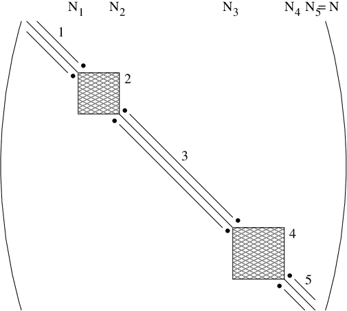
In the first step of the algorithm the full Hamiltonian appearing in the Green function is split into five smaller parts , referring to block respectively, and elements with connecting block and (with ), i.e.
| (19) |
We next define the projection operators on each block. Then we project the full Green function onto the block, whose elements we want to compute, thereby reducing the effort of inverting the full matrix to the inversion of an effective matrix of size and structure of block of the inverse Green function. We will exemplify this by calculating the elements of block 1 as well as those elements on the sub- and superdiagonal connecting block 1 and 2. Making subsequent use of the projection formula (14), we obtain
with . We calculate the elements of block 1 of the Green function by going through this hierarchy from bottom to top, having only to invert matrices of size and structure of the isolated blocks at each step. The computations for the other blocks of can be performed similarly.
The element can be calculated by splitting into and to write
with . After projecting onto the relevant block , one ends up with
The relevant elements of can be efficiently calculated using the algorithm introduced above for the blocks. Again the calculation of the other elements can be performed analogously.
For the calculation of the transmission probability (11) we need all matrix elements with and of the Green function . We use an algorithm which only requires the inversion of matrices of size and structure of the isolated blocks 1 to 5. We split the full Hamiltonian (19) into blocks and connecting elements and decompose
with . Multiplication with projection operators and yields
The elements of can be easily computed as the disconnected blocks of can be inverted individually. The elements , , , can be calculated by splitting into blocks and bonds and projecting onto the blocks needed. Details of the rather lengthy procedure can be found elsewhere [22].
References
References
- [1] Haldane F D M 1981 J. Phys. C: Solid State Phys.14 1585
- [2] For a short review of theory and experiment see Schönhammer K 2005 Luttinger Liquids: The Basic Concepts in Interacting Electrons in Low Dimensions ed D Baeriswyl (Dordrecht: Kluwer Academic Publishers)
- [3] Tans S J, Devoret M H, Dai H, Thess A, Smalley R E, Geerligs L J and Dekker C 1997 Nature(London) 386 474; Tans S J, Verschueren A R M and Dekker C 1998 Nature(London) 393 49; Auslaender O M, Yacoby A, de Picciotto R, Baldwin K W, Pfeiffer L N and West K W 2000 Phys. Rev. Lett.84 1764; Yao Z, Postma H W C, Balents L and Dekker C 1999 Nature(London) 402 273; Bockrath M, Cobden D H, Lu J, Rinzler A G, Smalley R E, Balents L and McEuen P L 1999 Nature(London) 397 598; Postma H W C, Teepen T, Yao Z, Grifoni M and Dekker C 2001 Science 293 76; de Picciotto R, Stormer H L, Pfeiffer L N, Baldwin K W and West K W 2001 Nature(London) 411 51; Gao B, Komnik A, Egger R, Glattli D C and Bachtold A 2004 Phys. Rev. Lett.92 216804
- [4] Sólyom J 1979 Adv. Phys. 28 201
- [5] Egger R and Gogolin A O 1997 Phys. Rev. Lett.79 5082; Kane C, Balents L and Fisher M P A 1997 Phys. Rev. Lett.79 5086
- [6] Meden V, Metzner W, Schollwöck U, Schneider O, Stauber T and Schönhammer K 2000 Eur. J. Phys.B 16 631
- [7] Yue D, Glazman L I and Matveev K A 1994 Phys. Rev.B 49 1966
- [8] Andergassen S, Enss T, Meden V, Metzner W, Schollwöck U and Schönhammer K 2006 Phys. Rev.B 73 045125
- [9] Kane C L and Fisher M P A 1992 Phys. Rev. Lett.68 1220; Kane C L and Fisher M P A 1992 Phys. Rev.B 46 7268; Kane C L and Fisher M P A 1992 Phys. Rev.B 46 15233
- [10] Fabrizio M and Gogolin A O 1995 Phys. Rev.B 51 17827
- [11] Enss T, Meden V, Andergassen S, Barnabé-Thériault X, Metzner W and Schönhammer K 2005 Phys. Rev.B 71 155401
- [12] Jakobs S G, Meden V, Schoeller H and Enss T 2007 Phys. Rev.B 75 035126
- [13] Maslov D L and Stone M 1995 Phys. Rev.B 52 R5539; Ponomarenko V V 1995 Phys. Rev.B 52 R8666; Safi I and Schulz H J 1995 Phys. Rev.B 52 R17040; Maslov D L 1995 Phys. Rev.B 52 R14368
- [14] Egger R and Grabert H 1996 Phys. Rev. Lett.77 538; Trauzettel B, Egger R and Grabert H 2002 Phys. Rev. Lett.88 116401
- [15] Jakobs S G, Meden V and Schoeller H 2007 Phys. Rev. Lett.99 150603
- [16] Andergassen S, Enss T, Meden V, Metzner W, Schollwöck U and Schönhammer K 2004 Phys. Rev.B 70 075102
- [17] Yang C N and Yang C P 1966 Phys. Rev.150 321; Yang C N and Yang C P 1966 Phys. Rev.150 327; Yang C N and Yang C P 1966 Phys. Rev.151 258
- [18] Haldane F D N 1980 Phys. Rev. Lett.45 1358
- [19] Oguri A 2001 J. Phys. Soc. Japan70 2666
- [20] See Imry Y 1997 Introduction to Mesoscopic Physics (Oxford: Oxford University Press) and references therein
- [21] Taylor J R 1972 Scattering Theory (New York: John Wiley and Sons)
- [22] For a detailed derivation see Wächter P (Ph.D. thesis, Universität Göttingen) in preparation.
- [23] Salmhofer M 1998 Renormalization (Berlin: Springer)
- [24] Salmhofer M and Honerkamp C 2001 Prog. Theor. Phys. 105 1
- [25] Meden V Lecture Notes, http://www.theorie.physik.uni-goettingen.de/meden/funRG/
- [26] Barnabé-Thériault X, Sedeki A, Meden V and Schönhammer K 2005 Phys. Rev.B 71 205327
- [27] Press W H, Teukolsky S A, Vetterling W T and Flannery B P 1992 Numerical Recipes in C (Cambridge: Cambridge Unviversity Press)
- [28] Details can be found in Enss T 2004 Renormalization, Conservation Laws and Transport in Correlated Electron Systems (Ph.D. thesis, Universität Stuttgart)