Maximum likelihood estimation of a multidimensional log-concave density
Abstract
Let be independent and identically distributed random vectors with a log-concave (Lebesgue) density . We first prove that, with probability one, there exists a unique maximum likelihood estimator of . The use of this estimator is attractive because, unlike kernel density estimation, the method is fully automatic, with no smoothing parameters to choose. Although the existence proof is non-constructive, we are able to reformulate the issue of computing in terms of a non-differentiable convex optimisation problem, and thus combine techniques of computational geometry with Shor’s -algorithm to produce a sequence that converges to . For the moderate or large sample sizes in our simulations, the maximum likelihood estimator is shown to provide an improvement in performance compared with kernel-based methods, even when we allow the use of a theoretical, optimal fixed bandwidth for the kernel estimator that would not be available in practice. We also present a real data clustering example, which shows that our methodology can be used in conjunction with the Expectation–Maximisation (EM) algorithm to fit finite mixtures of log-concave densities. An R version of the algorithm is available in the package LogConcDEAD – Log-Concave Density Estimation in Arbitrary Dimensions.
Keywords: Computational geometry, log-concavity, maximum likelihood estimation, non-differentiable convex optimisation, nonparametric density estimation, Shor’s -algorithm
1 Introduction
Modern nonparametric density estimation began with the introduction of a kernel density estimator in the pioneering work of Fix and Hodges (1951), later republished as Fix and Hodges (1989). For independent and identically distributed real-valued observations, the appealing asymptotic theory of the mean integrated squared error was provided by Rosenblatt (1956) and Parzen (1962). This theory leads to an asymptotically optimal choice of the smoothing parameter, or bandwidth. Unfortunately, however, it depends on the unknown density through the integral of the square of the second derivative of . Considerable effort has therefore been focused on finding methods of automatic bandwidth selection (cf. Wand and Jones, 1995, Chapter 3, and the references therein). Although this has resulted in algorithms, e.g. Chiu (1992), that achieve the optimal rate of convergence of the relative error, namely , where is the sample size, good finite sample performance is by no means guaranteed.
This problem is compounded when the observations take values in , where the general kernel estimator (Deheuvels, 1977) requires the specification of a symmetric, positive definite bandwidth matrix. The difficulties involved in making the choices for its entries mean that attention is often restricted either to bandwidth matrices that are diagonal, or even to those that are scalar multiples of the identity matrix. Of course, practical issues of automatic bandwidth selection remain.
In this paper, we propose a fully automatic nonparametric estimator of , with no tuning parameters to be chosen, under the condition that is log-concave – that is, is a concave function. The class of log-concave densities has many attractive properties and has been well-studied, particularly in the economics, sampling and reliability theory literature. See Section 2 for further discussion of examples, applications and properties of log-concave densities.
In Section 3, we show that if are independent and identically distributed random vectors with a log-concave density, then with probability one there exists a unique log-concave density that maximises the likelihood function,
Before continuing, it is worth noting that without any shape constraints on the densities under consideration, the likelihood function is unbounded. To see this, we could define a sequence of densities that represent successively close approximations to a mixture of ‘spikes’ (one on each ), such as , where denotes the density. This sequence satisfies as (cf. Figure 2). In fact, a modification of this argument may be used to show that the likelihood function remains unbounded even if we restrict attention to unimodal densities.


Figure 2 gives a diagram illustrating the structure of the maximum likelihood estimator on the logarithmic scale. This structure is most easily visualised for two-dimensional data, where one can imagine associating a ‘tent pole’ with each observation, extending vertically out of the plane. For certain tent pole heights, the graph of the logarithm of the maximum likelihood estimator can be thought of as the roof of a taut tent stretched over the tent poles. The fact that the logarithm of the maximum likelihood estimator is of this ‘tent function’ form constitutes part of the proof of its existence and uniqueness.
In Section 4, we discuss the computational problem of how to adjust the tent pole heights so that the corresponding tent functions converge to the logarithm of the maximum likelihood estimator. One reason that this computational problem is so challenging in more than one dimension is the fact that it is difficult to describe the set of tent pole heights that correspond to concave functions. The key observation, discussed in Section 4, is that it is possible to minimise a modified objective function that it is convex (though non-differentiable). This allows us to apply the powerful non-differentiable convex optimisation methodology of the subgradient method (Shor, 1985) and a variant called Shor’s -algorithm, which has been implemented by Kappel and Kuntsevich (2000).
As an illustration of the estimates obtained, Figure 3 presents plots of the maximum likelihood estimator, and its logarithm, for 1000 observations from a standard bivariate normal distribution. These plots were created using the LogConcDEAD package (Cule et al., 2008a) in R (R Development Core Team, 2008), which exploits the interactive surface-plotting software available in the rgl package (Adler and Murdoch, 2007).
In Section 5 we present simulations to compare the finite-sample performance of the maximum likelihood estimator with kernel-based methods. The results are striking: even when we use the theoretical, optimal bandwidth for the kernel estimator (or an asymptotic approximation to this when it is not available), we find that the maximum likelihood estimator has a rather smaller mean integrated squared error for moderate or large sample sizes, despite the fact that this optimal bandwidth depends on properties of the density that would be unknown in practice. This suggests that the maximum likelihood estimator is able to adapt to the local smoothness of the underlying density automatically.
Nonparametric density estimation is a fundamental tool for the visualisation of structure in exploratory data analysis, and has an enormous literature that includes the monographs of Devroye and Györfi (1985), Silverman (1986), Scott (1992) and Wand and Jones (1995). Our proposed method may certainly be used for this purpose; however, it may also be used as an intermediary stage in more involved statistical procedures. For instance:
- 1.
In classification problems, we have populations of interest, and assume in this discussion that these have densities on . We observe training data of the form , where if , then has density . The aim is to classify a new observation as coming from one of the populations. Problems of this type occur in a huge variety of applications, including medical diagnosis, archaeology, ecology etc. – see Gordon (1981), Hand (1981) or Devroye et al. (1996) for further details and examples. A natural approach to classification problems is to construct density estimates , where is based on the observations, say, from the th population, namely . We may then assign to the th population if . In this context, the use of kernel-based estimators in general requires the choice of separate bandwidth matrices, while the corresponding procedure based on the log-concave maximum likelihood estimates is again fully automatic.
- 2.
Clustering problems are closely related to the classification problems described above. The difference is that, in the above notation, we do not observe , and have to assign each of to one of the populations. A common technique is based on fitting a mixture density of the form , where the mixture proportions are positive and sum to one. Under the assumption that each of the component densities is log-concave, we show in Section 6 that our methodology can be extended to fit such a finite mixture density, which need not itself be log-concave – cf. Section 2. We also illustrate this clustering algorithm on a Wisconsin breast cancer data set in Section 6, where the aim is to separate observations into benign and malignant component populations.
- 3.
A functional of the true underlying density may be estimated by the corresponding functional of a density estimator, such as the log-concave maximum likelihood estimator. Examples of functionals of interest include probabilities, such as , moments, e.g. , and the differential entropy, . It may be possible to compute the plug-in estimator based on the log-concave maximum likelihood estimator analytically, but in Section 7, we show that even if this is not possible, in many cases of interest we can sample from the log-concave maximum likelihood estimator , and hence obtain a Monte Carlo estimate of the functional. This nice feature also means that the log-concave maximum likelihood estimator can be used in a Monte Carlo bootstrap procedure for assessing uncertainty in functional estimates – see Section 7 for further details.
- 4.
The fitting of a nonparametric density estimate may give an indication of the validity of a particular smaller model (often parametric). Thus, a contour plot of the log-concave maximum likelihood estimator may provide evidence that the underlying density has elliptical contours, and thus suggest that a model that exploits this elliptical symmetry.
- 5.
In the univariate case, Walther (2002) describes methodology based on log-concave density estimation for addressing the problem of detecting the presence of mixing in a distribution. As an application, he cites the Pickering/Platt debate (Swales, 1985) on the issue of whether high blood pressure is a disease (in which case observed blood pressure measurements should follow a mixture distribution), or simply a label attached to people in the right tail of the blood pressure distribution. As a result of our algorithm for computing the multidimensional log-concave maximum likelihood estimator, this methodology extends immediately to more than one dimension.
There has been considerable recent interest in shape-restricted nonparametric density estimation, but most of it has been confined to the case of univariate densities, where the computational algorithms are more straightforward. Nevertheless, as was discussed above, it is in multivariate situations that the automatic nature of the maximum likelihood estimator is particularly valuable. Walther (2002), Dümbgen and Rufibach (2007) and Pal et al. (2007) have proved the existence and uniqueness of the log-concave maximum likelihood estimator in one dimension and Dümbgen and Rufibach (2007), Pal et al. (2007) and Balabdaoui et al. (2008) have studied its theoretical properties. Rufibach (2007) has compared different algorithms for computing the univariate estimator, including the iterative convex minorant algorithm (Groeneboom and Wellner, 1992; Jongbloed, 1998), and three others. Dümbgen et al. (2007) also present an Active Set algorithm, which has similarities with the vertex direction and vertex reduction algorithms described in Groeneboom et al. (2008). For univariate data, it is also well-known that there exist maximum likelihood estimators of a non-increasing density supported on (Grenander, 1956) and of a convex, decreasing density (Groeneboom et al., 2001).
In Section 8, we give a brief concluding discussion, and suggest some directions for future research. Finally, we present in Appendix A a glossary of terms and results from convex analysis and computational geometry that appear in italics at their first occurrence in the main body of the paper; the references are Rockafellar (1997) and Lee (1997). Proofs are deferred to Appendix B, except that the beginning of the proof of Theorem 2 is given in the main text, as the ideas and notation introduced are needed in the remainder of the paper.
2 Log-concave densities: examples, applications and properties
Many of the most commonly-encountered parametric families of univariate distributions have log-concave densities, including the family of normal distributions, gamma distributions with shape parameter at least one, distributions with , Weibull distributions with shape parameter at least one, Gumbel, logistic and Laplace densities; see Bagnoli and Bergstrom (1989) for other examples. Univariate log-concave densities are unimodal and have fairly light tails – it may help to think of the exponential distribution (where the logarithm of the density is a linear function on the positive half-axis) as a borderline case. Thus Cauchy, Pareto and lognormal densities, for instance, are not log-concave. Mixtures of log-concave densities may be log-concave, but in general they are not; for instance, for , the location mixture of standard univariate normal densities is log-concave if and only if .
The assumption of log-concavity is a popular one in economics; Caplin and Naelbuff (1991b) show that in the theory of elections and under a log-concavity assumption, the proposal most preferred by the mean voter is unbeatable under a 64% majority rule. As another example, in the theory of imperfect competition, Caplin and Naelbuff (1991a) use log-concavity of the density of consumers’ utility parameters as a sufficient condition in their proof of the existence of a pure-strategy price equilibrium for any number of firms producing any set of products. See Bagnoli and Bergstrom (1989) for many other applications of log-concavity to economics. Brooks (1998) and Mengersen and Tweedie (1996) have exploited the properties of log-concave densities in studying the convergence of Markov chain Monte Carlo sampling procedures.
An (1998) lists many useful properties of log-concave densities. For instance, if and are (possibly multidimensional) log-concave densities, then their convolution is log-concave. In other words, if and are independent and have log-concave densities, then their sum has a log-concave density. The class of log-concave densities is also closed under the taking of pointwise limits. One-dimensional log-concave densities have increasing hazard functions, which is why they are of interest in reliability theory. Moreover, Ibragimov (1956) proved the following characterisation: a univariate density is log-concave if and only if the convolution is unimodal for every unimodal density . There is no natural generalisation of this result to higher dimensions.
As was mentioned in Section 1, this paper concerns multidimensional log-concave densities, for which fewer properties are known. It is therefore of interest to understand how the property of log-concavity in more than one dimension relates to the univariate notion. Our first proposition below is intended to give some insight into this issue. It is not formally required for the subsequent development of our methodology in Sections 3 and 4, although we did apply the result when designing our simulation study in Section 5. We assume throughout that log-concave densities are with respect to Lebesgue measure on the affine hull of their support, and ‘ has a log-concave density’ means ‘there exists a version of the density of that is log-concave’.
Proposition 1.
Let be a -variate random vector having density with respect to Lebesgue measure on . For a subspace of , let denote the orthogonal projection of onto . Then in order that be log-concave, it is:
- 1.
necessary that for any subspace , the marginal density of is log-concave and the conditional density of given is log-concave for each
- 2.
sufficient that for every -dimensional subspace , the conditional density of given is log-concave for each .
The part of Proposition 1(a) concerning marginal densities is an immediate consequence of Theorem 6 of Prékopa (1973). One can regard Proposition 1(b) as saying that a multidimensional density is log-concave if the restriction of the density to any line is a (univariate) log-concave function.
It is interesting to compare the properties of log-concave densities presented in Proposition 1 with the corresponding properties of Gaussian densities. In fact, Proposition 1 remains true if we replace ‘log-concave’ with ‘Gaussian’ throughout (at least, provided that in part (b) we also assume there is a point at which is twice differentiable). These shared properties suggest that the class of log-concave densities is a natural, infinite-dimensional generalisation of the class of Gaussian densities.
3 Existence, uniqueness and structure of the maximum likelihood estimator
Let denote the class of log-concave densities on with -dimensional support, and let . The degenerate case where the support is of dimension smaller than can also be handled, but for simplicity of exposition we concentrate on the non-degenerate case. Suppose that are a random sample from . We say that is a (nonparametric) maximum likelihood estimator of if it maximises over .
Theorem 2.
Suppose that . Then, with probability one, a nonparametric maximum likelihood estimator of exists and is unique.
First Part of Proof. We may assume that are distinct and their convex hull, , is a -dimensional polytope (an event of probability one when ). By a standard argument in convex analysis (Rockafellar, 1997, p. 37), for each there exists a function with the property that is the least concave function satisfying for all . Informally, is a ‘tent function’, and a typical example is depicted in Figure 2. Let denote ‘the class of tent functions’. Let denote the set of all log-concave functions on , and for , define
Suppose that maximises over . The main part of the proof, which is completed in the Appendix, consists of showing that
- (i)
for
- (ii)
for
- (iii)
- (iv)
- (v)
there exists such that if , then .
Although step (iii) above gives us a finite-dimensional class of functions to which belongs, the proof of Theorem 2 gives no indication of how to find the member of this class that maximises the likelihood function. We therefore seek an iterative algorithm to compute the estimator, but first we describe the structure we see in Figure 2 in Section 1 more precisely. From now on, we assume:
- (A1):
-
, and every subset of of size is affinely independent.
Note that when , the event in (A1) has probability one. From step (iii) in the proof of Theorem 2 above, there exists such that . As illustrated in Figure 2, and justified formally by Corollary 17.1.3 and Corollary 19.1.2 of Rockafellar (1997), the convex hull of the data, , may be triangulated in such a way that coincides with an affine function on each simplex in the triangulation. In other words, if is a -tuple of distinct indices in , and , then there exists a finite set consisting of such -tuples, with the following three properties:
- (i)
- (ii)
the relative interiors of the sets are pairwise disjoint
- (iii)
for some and . Here and below, denotes the usual Euclidean inner product in .
In the iterative algorithm that we propose in Section 4 for computing the maximum likelihood estimator, we need to find convex hulls and triangulations at each iteration. Fortunately, these can be computed efficiently using the Quickhull algorithm of Barber et al. (1996).
4 Computation of the maximum likelihood estimator
4.1 Reformulation
As a first attempt to find an algorithm which produces a sequence that converges to the maximum likelihood estimator in Theorem 2, it is natural to try to minimise numerically the function
Although this approach might work in principle, one difficulty is that is not convex, so this approach is extremely computationally intensive, even with relatively few observations. Another reason for the numerical difficulties stems from the fact that the set of -values on which attains its minimum is rather large: in general it may be possible to alter particular components without changing . Of course, we could have defined as a function of rather than as a function of the vector of tent pole heights . Our choice, however, motivates the following definition of a modified objective function:
| (4.1) |
The great advantages of minimising rather than are seen by the following theorem.
Theorem 3.
Assume (A1). The function is a convex function satisfying . It has a unique minimum at , say, and .
Thus Theorem 3 shows that the unique minimum of belongs to the minimum set of . In fact, it corresponds to the element of the minimum set for which for . Informally, then, is ‘a tent function with all of the tent poles touching the tent’.
In order to compute the function at a generic point , we need to be able to evaluate the integral in (4.1). In the notation of Section 3, we may write
For each , let be the matrix whose th column is for , and let . Then the affine transformation takes the unit simplex to . Letting , we can then establish by a simple change of variables and induction on that if are non-zero and distinct, then
| (4.2) |
Further details of this calculation can be found in a longer version of this paper (Cule et al., 2008b). The singularities that occur when some of may be zero or equal are removable. Thus, although (4.2) is a little complicated, it allows the computation of our objective function.
4.2 Nonsmooth optimisation
There is a vast literature on techniques of convex optimisation (cf. Boyd and Vandenberghe (2004), for example), including the method of steepest descent and Newton’s method. Unfortunately, these methods rely on the differentiability of the objective function, and the function is not differentiable. This can be seen informally by studying the schematic diagram in Figure 2 again. If the th tent pole, say, is touching but not critically supporting the tent, then decreasing the height of this tent pole does not change the tent function, and thus does not alter the integral in (4.1); on the other hand, increasing the height of the tent pole does alter the tent function and therefore the integral in (4.1). This argument may be used to show that at such a point, the th partial derivative of does not exist.
The set of points at which is not differentiable constitute a set of Lebesgue measure zero, but the non-differentiability cannot be ignored in our optimisation procedure. Instead, it will be necessary to derive a subgradient of at each point . This derivation, along with a more formal discussion of the non-differentiability of , can be found in the Appendix.
The theory of non-differentiable, convex optimisation is perhaps less well-known than its differentiable counterpart, but a fundamental contribution was made by Shor (1985) with his introduction of the subgradient method for minimising non-differentiable, convex functions defined on Euclidean spaces. A slightly specialised version of his Theorem 2.2 gives that if is a subgradient of at , then for any , the sequence generated by the formula
has the property that either there exists an index such that , or and as , provided we choose the step lengths so that as , but .
Shor recognised, however, that the convergence of this algorithm could be slow in practice, and that although appropriate step size selection could improve matters somewhat, the convergence would never be better than linear (compared with quadratic convergence for Newton’s method near the optimum – see Boyd and Vandenberghe (2004, Section 9.5)). Slow convergence can be caused by taking at each stage a step in a direction nearly orthogonal to the direction towards the optimum, which means that simply adjusting the step size selection scheme will never produce the desired improvements in convergence rate.
One solution (Shor, 1985, Chapter 3) is to attempt to shrink the angle between the subgradient and the direction towards the minimum through a (necessarily nonorthogonal) linear transformation, and perform the subgradient step in the transformed space. By analogy with Newton’s method for smooth functions, an appropriate transformation would be an approximation to the inverse of the Hessian matrix at the optimum. This is not possible for nonsmooth problems, because the inverse might not even exist (and will not exist at points at which the function is not differentiable, which may include the optimum).
Instead, we perform a sequence of dilations in the direction of the difference between two successive subgradients, in the hope of improving convergence in the worst-case scenario of steps nearly perpendicular to the direction towards the minimiser. This variant, which has become known as Shor’s -algorithm, has been implemented in Kappel and Kuntsevich (2000). Accompanying software SolvOpt is available from http://www.uni-graz.at/imawww/kuntsevich/solvopt/.
Although the formal convergence of the -algorithm has not been proved, we agree with the authors’ claims that it is robust, efficient and accurate. Of course, it is clear that if we terminate the -algorithm after any finite number of steps and apply the original Shor algorithm using our terminating value of as the new starting value, then formal convergence is guaranteed. We have not found it necessary to run the original Shor algorithm after termination of the -algorithm in practice.
If denotes the sequence of vectors in produced by the -algorithm, we terminate when
- •
- •
for
- •
for some small . The first two termination criteria follow Kappel and Kuntsevich (2000), while the third is based on our knowledge that the true optimum corresponds to a density (Section 3). As default values, and throughout this paper, we took and .
Table 1 gives approximate running times and number of iterations of Shor’s -algorithm required for different sample sizes and dimensions on an ordinary desktop computer (1.8GHz, 2GB RAM). Unsurprisingly, the running time increases relatively quickly with the sample size, while the number of iterations increases approximately linearly with . Each iteration takes longer as the dimension increases, though it is interesting to note that the number of iterations required for the algorithm to terminate decreases as the dimension increases. When , we recommend the Active Set algorithm of Dümbgen et al. (2007), which is implemented in the R package logcondens (Rufibach and Dümbgen, 2006).
| 1.5 secs (260) | 50 secs (1270) | 4 mins (2540) | 24 mins (5370) | |
| 6 secs (170) | 100 secs (820) | 7 mins (1530) | 44 mins (2740) | |
| 23 secs (135) | 670 secs (600) | 37 mins (1100) | 224 mins (2060) |
5 Finite sample performance
| LogConcDEAD | Kernel (opt MISE) | Kernel (LSCV) | |
| 100 | 0.00620(0.000222) | 0.00431 | 0.00622(0.000383) |
| 500 | 0.00161(0.0000514) | 0.00164 | 0.00199(0.0000844) |
| 1000 | 0.000983(0.0000289) | 0.00106 | 0.00122(0.0000495) |
| 2000 | 0.000599(0.0000155) | 0.000686 | 0.000803(0.0000276) |
| LogConcDEAD | Kernel (opt MISE) | Kernel (LSCV) | |
| 100 | 0.00607(0.000283) | 0.00440 | 0.00827(0.000583) |
| 500 | 0.00168(0.0000573) | 0.00167 | 0.00240(0.000122) |
| 1000 | 0.00100(0.0000295) | 0.00108 | 0.00142(0.0000662) |
| 2000 | 0.000608(0.0000154) | 0.000700 | 0.000868(0.0000331) |
| LogConcDEAD | Kernel (opt AMISE) | Kernel (LSCV) | |
| 100 | 0.00588(0.000222) | 0.00644 | 0.00800(0.000339) |
| 500 | 0.00143(0.0000478) | 0.00220 | 0.00291(0.0000687) |
| 1000 | 0.000802(0.0000236) | 0.00139 | 0.00194(0.0000456) |
| 2000 | 0.000451(0.0000110) | 0.000874 | 0.00130(0.0000209) |
| LogConcDEAD | Kernel (opt MISE) | Kernel (LSCV) | |
| 100 | 0.00504(0.000206) | 0.00384 | 0.00515(0.000195) |
| 500 | 0.00136(0.0000745) | 0.00145 | 0.00179(0.0000515) |
| 1000 | 0.000747(0.0000622) | 0.000945 | 0.00116(0.0000376) |
| 2000 | 0.000543(0.0000553) | 0.000610 | 0.000683(0.0000121) |
| LogConcDEAD | Kernel (opt MISE) | Kernel (LSCV) | |
| 100 | 0.00434(0.00158) | 0.00304 | 0.00514(0.000322) |
| 500 | 0.000996(0.0000622) | 0.00117 | 0.00146(0.000442) |
| 1000 | 0.000640(0.0000502) | 0.000760 | 0.000880(0.000176) |
| 2000 | 0.000445(0.0000455) | 0.000492 | 0.000583(0.0000192) |
| LogConcDEAD | Kernel (opt MISE) | Kernel (LSCV) | |
| 100 | 0.00467(0.000139) | 0.00326 | 0.00484(0.000244) |
| 500 | 0.00173(0.0000522) | 0.00126 | 0.00150(0.000363) |
| 1000 | 0.00122(0.0000456) | 0.000819 | 0.000925(0.0000131) |
| 2000 | 0.00105(0.0000340) | 0.000530 | 0.000577(0.0000651) |
| LogConcDEAD | Kernel (opt MISE) | Kernel (LSCV) | |
| 100 | 0.00426(0.000131) | 0.00240 | 0.00505(0.000279) |
| 500 | 0.000835(0.0000302) | 0.00106 | 0.00143(0.0000338) |
| 1000 | 0.000442(0.0000236) | 0.000737 | 0.000888(0.0000139) |
| 2000 | 0.000304(0.0000238) | 0.000508 | 0.000579(0.00000985) |
| LogConcDEAD | Kernel (opt MISE) | Kernel (LSCV) | |
| 100 | 0.00467(0.000147) | 0.00254 | 0.00550(0.000361) |
| 500 | 0.000812(0.0000301) | 0.00112 | 0.00152(0.0000367) |
| 1000 | 0.000431(0.0000249) | 0.000778 | 0.000922(0.0000145) |
| 2000 | 0.000304(0.0000233) | 0.000537 | 0.000603(0.00000676) |
| LogConcDEAD | Kernel (opt AMISE) | Kernel (LSCV) | |
| 100 | 0.00365(0.000142) | 0.00344 | 0.0741(0.00400) |
| 500 | 0.000779(0.0000243) | 0.00136 | 0.00192(0.0000518) |
| 1000 | 0.000538(0.000104) | 0.000922 | 0.00123(0.0000262) |
| 2000 | 0.000292(0.0000414) | 0.000622 | 0.000849(0.0000228) |
| LogConcDEAD | Kernel (opt MISE) | Kernel (LSCV) | |
| 100 | 0.00395(0.000124) | 0.00214 | 0.00446(0.000242) |
| 500 | 0.000743(0.0000272) | 0.000946 | 0.00124(0.0000298) |
| 1000 | 0.000446(0.0000218) | 0.000656 | 0.000822(0.0000179) |
| 2000 | 0.000265(0.0000202) | 0.000452 | 0.000508(0.00000537) |
| LogConcDEAD | Kernel (opt MISE) | Kernel (LSCV) | |
| 100 | 0.00319(0.000100) | 0.00168 | 0.00371(0.000203) |
| 500 | 0.000596(0.0000231) | 0.000748 | 0.00103(0.0000340) |
| 1000 | 0.000329(0.0000173) | 0.000520 | 0.000656(0.0000160) |
| 2000 | 0.000220(0.0000171) | 0.000358 | 0.000410(0.00000519) |
| LogConcDEAD | Kernel (opt MISE) | Kernel (LSCV) | |
| 100 | 0.00328(0.0000930) | 0.00166 | 0.00296(0.000120) |
| 500 | 0.000803(0.0000184) | 0.000751 | 0.000998(0.000254) |
| 1000 | 0.000552(0.0000169) | 0.000525 | 0.000613(0.0000892) |
| 2000 | 0.000401(0.0000133) | 0.000364 | 0.000404(0.00000488) |
Our simulation study considered, for and , the following densities:
- (a)
standard normal,
- (b)
dependent normal, , with
- (c)
the joint density of independent components
- (d-f)
the normal location mixture for (d) , (e) , (f) . An application of Proposition 1 gives that such a normal location mixture is log-concave if and only if .
In Tables 2 and 3 we present, for each density and for four different sample sizes, an estimate of the mean integrated squared error (MISE) of the nonparametric maximum likelihood estimator based on 100 Monte Carlo iterations. We also show the MISE for the kernel density estimates with a Gaussian kernel and, for all of the normal and mixture of normal examples, the choice of bandwidth that minimises the MISE. In the gamma example, exact MISE calculations are not possible, so we took the bandwidth that minimises the asymptotic mean integrated squared error (AMISE). These optimal bandwidths can be computed using the formulae in Wand and Jones (1995, Sections 4.3 and 4.4). As minimisation of the expressions for both the MISE and the AMISE requires knowledge of certain functionals of the true density that would be unknown in practice, we also provide a comparison with an empirical bandwidth selector based on least squares cross validation (LSCV) (Wand and Jones, 1995, Section 4.7). The LSCV bandwidths were computed using the ks package (Duong, 2007) in R, and we used the option of constraining the bandwidth matrices to be diagonal in cases (a) and (c) where the components are independent.
We see that in cases (a)-(e) the log-concave maximum likelihood estimator has a smaller MISE than the kernel estimate with bandwidth chosen by LSCV, and at least for moderate and large sample sizes, the difference is quite dramatic. Even more remarkably, in these cases the log-concave estimator also outperforms the kernel estimate with optimally chosen bandwidth when the sample size is not too small. It seems that for small sample sizes, the fact that the convex hull of the data is rather small hinders the performance of the log-concave estimator, but that this effect is reduced as the sample size increases. The log-concave estimator copes well with the dependence in case (b), and it also deals particularly impressively with case (c), where the true density decays to zero at the boundary of the positive orthant.
In case (f), where the log-concavity assumption is violated, the performance of our estimator is not as good as the kernel estimate with the optimally chosen bandwidth, but is still comparable in most cases with the LSCV method. One would not expect the MISE of to approach zero as if log-concavity is violated, and in fact we conjecture that in this case the log-concave maximum likelihood estimator will converge to the density that minimises the Kullback–Leibler divergence over . Such a result would be interesting for robustness purposes, because it could be interpreted as saying that provided the underlying density does not violate the log-concavity assumption too seriously, the log-concave maximum likelihood estimator is still sensible.
6 Clustering example
In a recent paper, Chang and Walther (2008) introduced an algorithm which combines the univariate log-concave maximum likelihood estimator with the EM algorithm (Dempster et al., 1977), to fit a finite mixture density of the form
| (6.1) |
where the mixture proportions are positive and sum to one, and the component densities are univariate and log-concave. The method is an extension of the standard Gaussian EM algorithm, e.g. Fraley and Raftery (2002), which assumes that each component density is normal. Once estimates have been obtained, clustering can be carried out by assigning to the th cluster those observations for which . Chang and Walther (2008) show empirically that in cases where the true component densities are log-concave but not normal, their algorithm tends to make considerably fewer misclassifications and have smaller mean absolute error in the mixture proportion estimates than the Gaussian EM algorithm, with very similar performance in cases where the true component densities are normal.
Owing to the previous lack of an algorithm for computing the maximum likelihood estimator of a multidimensional log-concave density, Chang and Walther (2008) discuss an extension of the model in (6.1) to a multivariate context where the univariate marginal densities of each component in the mixture are assumed to be log-concave, and the dependence structure within each component density is modelled with a normal copula. Now that we are able to compute the maximum likelihood estimator of a multidimensional log-concave density, we can carry this method through to its natural conclusion. That is, in the finite mixture model (6.1) for a multidimensional log-concave density , we simply assume that each of the component densities is log-concave. An interesting problem that we do not address here that of finding appropriate conditions under which this model is identifiable – see Titterington et al. (1985, Section 3.1) for a nice discussion.
6.1 EM algorithm
An introduction to the EM algorithm can be found in McLachlan and Krishnan (1997). Briefly, given current estimates of the mixture proportions and component densities at the th iteration of the algorithm, we update the estimates of the mixture proportions by setting for , where
is the current estimate of the posterior probability that the th observation belongs to the th component. We then update the estimates of the component densities in turn using the algorithm described in Section 4, choosing to be the log-concave density that maximises
The incorporation of the weights in the maximisation process presents no additional complication, as is easily seen by inspecting the proof of Theorem 2. As usual with methods based on the EM algorithm, although the likelihood increases at each iteration, there is no guarantee that the sequence converges to a global maximum. In fact, it can happen that the algorithm produces a sequence that approaches a degenerate solution, corresponding to a component concentrated on a single observation, so that the likelihood becomes arbitrarily high. The same issue can arise when fitting mixtures of Gaussian densities, and in this context Fraley and Raftery (2002) suggest that a Bayesian approach can alleviate the problem in these instances by effectively smoothing the likelihood. In general, it is standard practice to restart the algorithm from different initial values, taking the solution with the highest likelihood.
6.2 Breast cancer example
We illustrate the log-concave EM algorithm on the Wisconsin breast cancer data set of Street et al. (1993), available on the UCI Machine Learning Repository website (Asuncion and Newman, 2007):
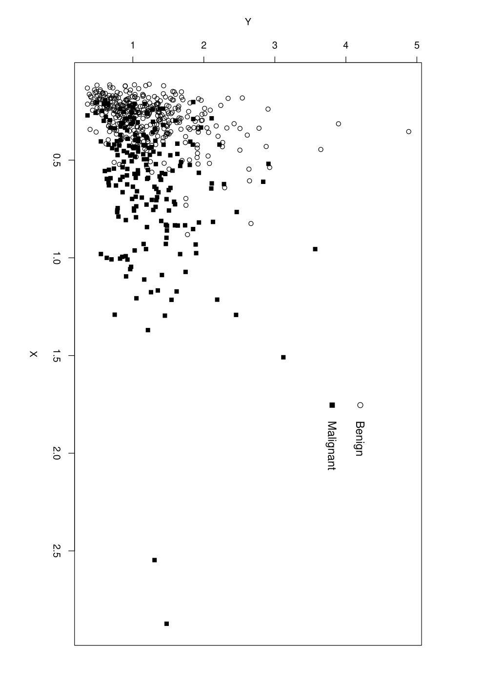


The data set was created by taking measurements from a digitised image of a fine needle aspirate of a breast mass, for each of 569 individuals, with 357 benign and 212 malignant instances. We study the problem of trying to diagnose (cluster) the individuals based on the standard errors of two of the measurements, namely the radius of the cell nucleus (mean of distances from center to points on the perimeter, ) and its texture (standard deviation of grey-scale values, ). The data are presented in Figure 4(a). In fact, the full data set consists of 30 measurements for each patient, representing the mean, standard error and ‘worst’ (mean of the three largest values) of 10 different features computed for each cell nucleus in the image. Since one would reasonably expect the means of each feature to be approximately normally distributed, and hence the Gaussian EM algorithm to be appropriate, we took the standard errors of the first two measurements to illustrate the log-concave EM algorithm methodology.
It is important also to note that although for this particular data set we do know whether a particular instance is benign or malignant, we did not use this information in fitting our mixture model. Instead this information was only used afterwards to assess the performance of the method, as reported below. Thus we are studying a clustering (or unsupervised learning) problem, by taking a classification (or supervised learning) data set and ‘covering up the labels’ until it comes to performance assessment.
The skewness in the data suggests that the mixture of Gaussians model may be inadequate, and in Figure 4(b) we show the contour plot and misclassified instances from this model. The corresponding plot obtained from the log-concave EM algorithm is given in Figure 4(c), while Figure 4(d) plots the fitted mixture distribution from the log-concave EM algorithm. For this example, the number of misclassified instances is reduced from 144 with the Gaussian EM algorithm to 121 with the log-concave EM algorithm.
In some examples, it will be necessary to estimate , the number of mixture components. In the general context of model-based clustering, Fraley and Raftery (2002) cite several possible approaches for this purpose, including methods based on resampling (McLachlan and Basford, 1988) and an information criterion (Bozdogan, 1994). Further research will be needed to ascertain which of these methods is most appropriate in the context of log-concave component densities.
7 Plug-in estimation of functionals, sampling and the bootstrap
Suppose has density . Often, we are less interested in estimating a density directly than in estimating some functional . Examples of functionals of interest (some of which were given in Section 1), include:
- (a)
- (b)
Moments, such as , or
- (c)
The differential entropy of (or ), defined by
- (d)
The highest density region, defined by , where is the largest constant such that . Hyndman (1996) argues that this is an informative summary of a density; note that subject to a minor restriction on , we have .
Each of these may be estimated by the corresponding functional of the log-concave maximum likelihood estimator. In examples (a) and (b) above, may also be written as a functional of the corresponding distribution function , e.g. . In such cases, it is more natural to use the plug-in estimator based on the empirical distribution function, , of the sample , and indeed in our simulations we found that the log-concave plug-in estimator did not offer an improvement on this method. In the other examples, however, an empirical distribution function plug-in estimator is not available, and the log-concave plug-in estimator is a potentially attractive procedure.
7.1 Monte Carlo estimation of functionals and sampling from the density estimate
For some functionals we can compute analytically. If this is not possible, but we can write , we may approximate by
for some (large) , where are independent samples from . Conditional on , the strong law of large numbers gives that as . In practice, even when analytic calculation of was possible, this method was found to be fast and accurate.
In order to use this Monte Carlo procedure, we must be able to sample from . Fortunately, this can be done efficiently using the following rejection sampling procedure. As in Section 4, for let be the matrix whose th column is for , and let , so that maps the unit simplex to . Recall that , and let , where for . Write
We may then draw an observation from as follows:
- (i)
Select , selecting with probability
- (ii)
Select and independently. If
accept the point and set . Otherwise, repeat (ii).
7.2 Simulation study
In this section we illustrate some simple applications of this technique to functionals (c) and (d) above, using the Monte Carlo procedure and sampling scheme described in Section 7.1. Estimates are based on random samples from a distribution, and we compare the performance of the LogConcDEAD estimate with that of a kernel-based plug-in estimate, where the bandwidth matrix was chosen using our knowledge of the underlying density to minimise the MISE.
Table 4(a) gives mean squared errors (with Monte Carlo standard errors) of the plug-in estimates of the differential entropy. In Table 4(b) we study the plug-in estimators of the highest density region , and measure the quality of the estimation procedures through , where and denotes set difference. Highest density regions can be computed once we have approximated the sample versions of using the density quantile algorithm described in Hyndman (1996, Section 3.2).
For the differential entropy estimators, we find a similar pattern to that observed in Section 5: the log-concave plug-in estimator provides an improvement on the kernel-based estimator for the moderate and large sample sizes in our simulations. For the case of highest density regions, the relative performance of the log-concave estimator is better for the estimation of smaller density regions. In Figure 5, we illustrate the estimation of three highest density regions based on 500 points from a distribution. For comparison, a kernel-based plug-in estimate (where the regions are not guaranteed to be convex) is also given.
| LogConcDEAD | Kernel | |
| 100 | 0.0761(0.00629) | 0.0457(0.00304) |
| 500 | 0.00819(0.000653) | 0.0137(0.000839) |
| 1000 | 0.00378(0.000391) | 0.00716(0.000581) |
| 2000 | 0.00177(0.000232) | 0.00427(0.000345) |
| LogConcDEAD | Kernel | |
| 100 | 0.0872(0.0024)/0.110(0.0033)/0.121(0.0047) | 0.0753(0.0017)/0.0995(0.0028)/0.0959(0.0038) |
| 500 | 0.0419(0.0010)/0.0587(0.0014)/0.0680(0.0022) | 0.0467(0.0011)/0.0609(0.0013)/0.0637(0.0019) |
| 1000 | 0.0311(0.00075)/0.0447(0.0011)/0.0536(0.0016) | 0.0376(0.00095)/0.0476(0.0012)/0.0477(0.0015) |
| 2000 | 0.0241(0.00054)/0.0363(0.00080)/0.0448(0.0013) | 0.0322(0.00081)/0.0371(0.00098)/0.0399(0.0013) |


In real data examples, we are unable to assess uncertainty in our functional estimates by taking repeated samples from the true underlying model. Nevertheless, the fact that we can sample from the log-concave maximum likelihood estimator does mean that we can apply standard bootstrap methodology to compute standard errors or confidence intervals, for example. Finally, we remark that the plug-in estimation procedure, sampling algorithm and bootstrap methodology extend in an obvious way to the case of a finite mixture of log-concave densities.
8 Concluding discussion
We have developed methodology that gives a fully automatic nonparametric density estimate under the condition that the density is log-concave, and shown how it may be extended to fit finite mixtures of log-concave densities. We have indicated a wide range of possible applications, including classification, clustering and functional estimation problems. The area of shape-constrained estimation is currently undergoing rapid growth, as evidenced by the many recent publications cited in the penultimate paragraph of Section 1, as well as recent workshops in Oberwolfach (November 2006), Eindhoven (October 2007) and Bristol (November 2007). We hope that this paper will stimulate further interest and research in the field.
As well as the continued development and refinement of the computational algorithms and graphical displays of estimates, and studies of theoretical performance, there remain many challenges and interesting directions for future research. These include:
- (i)
Studying other shape constraints. These have received some attention for univariate data, dating back to Grenander (1956), but much less in the multivariate setting.
- (ii)
Developing both formal and informal diagnostic tools for assessing the validity of shape constraints.
- (iii)
Assessing the uncertainty in shape-constrained nonparametric density estimates, through confidence intervals/bands.
- (iv)
Developing analogous methodology for discrete data from shape-constrained distributions.
- (v)
Examining nonparametric shape constraints in regression problems.
- (vi)
Studying methods for choosing the number of clusters in nonparametric, shape-constrained mixture models.
Appendix A Glossary of terms and results from convex analysis and computational geometry
All of the definitions and results below can be found in Rockafellar (1997) and Lee (1997). The epigraph of a function is the set
We say is concave if its epigraph is non-empty and convex as a subset of ; note that this agrees with the terminology of Barndorff-Nielsen (1978), but is what Rockafellar (1997) calls a proper concave function. If is a convex subset of then provided is not identically , it is concave if and only if
for and . A non-negative function is log-concave if is concave, with the convention that . The support of a log-concave function is , a convex subset of .
A subset of is affine if for all and . The affine hull of , denoted , is the smallest affine set containing . Every non-empty affine set in is parallel to a unique subspace of , meaning that there is a unique subspace of such that , for some . The dimension of is the dimension of this subspace, and more generally the dimension of a non-empty convex set is the dimension of its affine hull. A finite set of points is affinely independent if is -dimensional. The relative interior of a convex set is the interior which results when we regard as a subset of its affine hull. The relative boundary of is the set difference between its closure and its relative interior. If is an affine set in , then an affine transformation (or afffine function) is a function such that for all and .
The closure of a concave function on , denoted , is the function whose epigraph is the closure in of . It is the least upper semi-continuous, concave function satisfying . The function is closed if . An arbitrary function on is continuous relative to a subset of if its restriction to is a continuous function. A non-zero vector is a direction of increase of on if is non-decreasing for every .
The convex hull of finitely many points is called a polytope. The convex hull of affinely independent points is called a -dimensional simplex (pl. simplices). If is a convex set in , then a supporting half-space to is a closed half-space which contains and has a point of in its boundary. A supporting hyperplane to is a hyperplane which is the boundary of a supporting half-space to . Thus , for some and such that for all with equality for at least one .
If is a finite set of points in such that is a -dimensional polytope in , then a face of is a set of the form , where is a supporting hyperplane to . The vertex set of , denoted , is the set of -dimensional faces (vertices) of . A subdivision of is a finite set of -dimensional polytopes such that is the union of and the intersection of any two distinct polytopes in the subdivision is a face of both of them. If and are two subdivisions of , then is a refinement of if each is contained in some . The trivial subdivision of is . A triangulation of is a subdivision of in which each polytope is a simplex.
If is a -dimensional polytope in , is a -dimensional face of and , then there is a unique supporting hyperplane to containing . The polytope is contained in exactly one of the closed half-spaces determined by , and if is in the opposite open half-space, then is visible from . If is a finite set in such that , if and is a subdivision of , then the result of pushing is the subdivision of obtained by modifying each as follows:
- (i)
If , then
- (ii)
If and is -dimensional, then
- (iii)
If and is -dimensional, then . Also, if is any -dimensional face of that is visible from , then .
If is a convex function on , then is a subgradient of at if
for all . If is differentiable at , then is the unique subgradient to at ; otherwise the set of subgradients at has more than one element. The one-sided directional derivative of at with respect to is
which always exists (allowing and as limits) provided is finite.
Appendix B Proofs
Proof of Proposition 1
(a) If is log-concave, then for , we can write
a product of log-concave functions. Thus is log-concave for each .
(b) Let be distinct and let . Let be the -dimensional subspace of whose orthogonal complement is parallel to the affine hull of (i.e. the line through and ). Writing for the marginal density of and for the common value of and , the density of at is
Thus is log-concave, as required.
Completion of the Proof of
Theorem 2
We prove each of the steps (i)–(v)
outlined in Section 3 in turn. First note that if
, then by Carathéodory’s theorem (Theorem 17.1 of
Rockafellar (1997)), there exist distinct indices
with , such that with each and . Thus, if , then by Jensen’s inequality,
so for some . But then . This proves (i).
Now suppose for some . Then is a convex set containing , a set which has strictly larger -dimensional Lebesgue measure than that of . We therefore have , which proves (ii).
To prove (iii), we first show that is closed. Suppose that for but that . Then since for all , we may assume that there exists such that . If is in the relative interior of , then since and are continuous at (by Theorem 10.1 of Rockafellar (1997)), we must have
The only remaining possibility is that is on the relative boundary of . But is closed by Corollary 17.2.1 of Rockafellar (1997), so writing for the closure of a concave function , we have , where we have used Corollary 7.3.4 of Rockafellar (1997) to obtain the middle equality. It follows that is closed and , which proves (iii).
Note that has no direction of increase, because if , is a non-zero vector and is large enough that , then . It follows by Theorem 27.2 of Rockafellar (1997) that the supremum of is finite (and is attained). Using properties (i) and (ii) as well, we may write , say, where . Thus , for some . But then
with equality only if . This proves (iv).
To prove (v), we may assume by (iv) that is a density. Let and let . We show that when is large, in order for to be a density, must be negative with so large that . First observe that if and , then for sufficiently large we must have , and then
(The fact that follows by Jensen’s inequality.) Hence, denoting Lebesgue measure on by , we have
Thus
For to be a density, then, we require when is large. But then
when is sufficiently large. This proves (v).
It is not hard to see that for any , the function is continuous on the compact set , and thus the proof of the existence of a maximum likelihood estimator is complete. To prove uniqueness, suppose that and both and maximise . We may assume , and and are supported on . Then the normalised geometric mean
is a log-concave density, with
However, by Cauchy–Schwarz, , so . Equality is obtained if and only if almost everywhere, but since and are continuous relative to (Theorem 10.2 of Rockafellar (1997)), this implies that . An alternative way of proving the uniqueness of the maximum likelihood estimator may be based on the fact that for all , provided and are distinct elements of .
Proof of Theorem 3
For and , the function
is the least concave function
satisfying for , so
. The convexity of follows from this
and the convexity of the exponential function. It is clear that
, since for
.
From Theorem 2, we can find such that with for , and this minimises . For any other which minimises , by the uniqueness part of Theorem 2 we must have , so .
B.1 Non-differentiability of and computation of subgradients
In this section, we find explicitly the set of points at which the function defined in (4.1) is differentiable, and compute a subgradient of at each point. For , define
The set is the index set of those simplices that have as a vertex. Let denote the set of vectors with the property that for each , if for any then
is affinely independent in . This is the set of points for which no tent pole is touching but not critically supporting the tent. Notice that the complement of has zero Lebesgue measure in . For and , and in the notation of Section 4, let
Proposition 4.
Assume (A1). (a) For , the function is differentiable at and for satisfies
(b) For , the function is not differentiable at , but the vector is a subgradient of at .
Proof.
By Theorem 25.2 of Rockafellar (1997), it suffices to show that for , all of the partial derivatives exist and are given by the expression in the statement of the proposition. For and , let , where denotes the th unit coordinate vector in . For sufficiently small values of , we may write
for certain values of and . If , then and for sufficiently small . On the other hand, if , then there are two cases to consider:
- (i)
If , then for sufficiently small , we have , where denotes a -vector of ones, so that and
- (ii)
If for some , then for sufficiently small , we have , so that and .
It follows that
where to obtain the final line we have made the substitution , after taking the limit as .
(b) If , then it can be shown that there exists a unit coordinate vector in such that the one-sided directional derivative at with respect to , denoted , satisfies . Thus is not differentiable at . To show that is a subgradient of at , it is enough by Theorem 25.6 of Rockafellar (1997) to find, for each , a point such that and such that is differentiable at with . This can be done by sequentially making small adjustments to the components of in the same order as that in which the vertices were pushed in constructing the triangulation. ∎
A subgradient of at any may be computed using Proposition 4, (B.1) and (4.2) once we have a formula for
when are non-zero and distinct. In Cule et al. (2008b), it is shown that the required formula is
| (B.1) |
References
- Adler and Murdoch (2007) Adler, D. and Murdoch, D. (2007) rgl: 3D visualization device system (OpenGL). URL http://rgl.neoscientists.org. R package version 0.75.
- An (1998) An, M. Y. (1998) Logconcavity versus logconvexity: A complete characterization. J. Econom. Theory, 80, 350–369.
- Asuncion and Newman (2007) Asuncion, A. and Newman, D. J. (2007) UCI Machine Learning Repository. URL http://www.ics.uci.edu/~mlearn/MLRepository.html.
- Bagnoli and Bergstrom (1989) Bagnoli, M. and Bergstrom, T. (1989) Log-concave probability and its applications. Unpublished manuscript.
- Balabdaoui et al. (2008) Balabdaoui, F., Rufibach, K. and Wellner, J. A. (2008) Maximum likelihood estimation of a logconcave density and its distribution function. URL arXiv:0708.3400v2. Preprint.
- Barber et al. (1996) Barber, C. B., Dobkin, D. P. and Huhdanpaa, H. (1996) The quickhull algorithm for convex hulls. ACM Trans. Math. Software, 22, 469–483. URL http://www.qhull.org.
- Barndorff-Nielsen (1978) Barndorff-Nielsen, O. (1978) Information and Exponential Families in Statistical Theory. New York: Wiley.
- Boyd and Vandenberghe (2004) Boyd, S. and Vandenberghe, L. (2004) Convex Optimization. Cambridge University Press.
- Bozdogan (1994) Bozdogan, H. (1994) Choosing the number of clusters, subset selection of variables, and outlier detection on the standard mixture-model cluster analysis. In New Approaches in Classification and Data Analysis (eds. E. Diday, Y. Lechevallier, M. Schader, P. Bertrand and B. Burtschy), 169–177. New York: Springer-Verlag.
- Brooks (1998) Brooks, S. P. (1998) MCMC convergence diagnosis via multivariate bounds on log-concave densities. Ann. Statist., 26, 398–433.
- Caplin and Naelbuff (1991a) Caplin, A. and Naelbuff, B. (1991a) Aggregation and imperfect competition: On the existence of equilibrium. Econometrica, 25–59.
- Caplin and Naelbuff (1991b) Caplin, A. and Naelbuff, B. (1991b) Aggregation and social choice: A mean voter theorem. Econometrica, 1–23.
- Chang and Walther (2008) Chang, G. and Walther, G. (2008) Clustering with mixtures of log-concave distributions. Computational Statistics and Data Analysis. To appear.
- Chiu (1992) Chiu, S.-T. (1992) An automatic bandwidth selector for kernel density estimation. Biometrika, 79, 771–782.
- Cule et al. (2008a) Cule, M., Gramacy, R. and Samworth, R. (2008a) LogConcDEAD: Maximum likelihood estimation of a log-concave density. R package version 1.1-0.
- Cule et al. (2008b) Cule, M. L., Samworth, R. J. and Stewart, M. I. (2008b) Maximum likelihood estimation of a multidimensional log-concave density. Available at http://www.statslab.cam.ac.uk/~rjs57/Research.html.
- Deheuvels (1977) Deheuvels, P. (1977) Estimation non parametrique de la densité par histogrammes generalisés II. Publ. l’Inst. Statist. l’Univ Paris, 22, 1–23.
- Dempster et al. (1977) Dempster, A., Laird, N. and Rubin, D. (1977) Maximum likelihood from incomplete data via the EM algorithm. J. Roy. Statist. Soc., Ser. B, 39, 1–38.
- Devroye and Györfi (1985) Devroye, L. and Györfi, L. (1985) Nonparametric Density Estimation : The View. New York: Wiley.
- Devroye et al. (1996) Devroye, L., Györfi, L. and Lugosi, G. (1996) A Probabilistic Theory of Pattern Recognition. New York: Springer.
- Dümbgen et al. (2007) Dümbgen, L., Hüsler, A. and Rufibach, K. (2007) Active set and em algorithms for log-concave densities based on complete and censored data. URL arXiv:0709.0334v2. Preprint.
- Dümbgen and Rufibach (2007) Dümbgen, L. and Rufibach, K. (2007) Maximum likelihood estimation of a log-concave density: basic properties and uniform consistency. URL arXiv:0709.0334v2. Preprint.
- Duong (2007) Duong, T. (2007) ks: Kernel smoothing. URL http://web.maths.unsw.edu.au/~tduong. R package version 1.4.11.
- Fix and Hodges (1951) Fix, E. and Hodges, J. L. (1951) Discriminatory analysis – nonparametric discrimination: Consistency properties. Tech. Rep. 4, Project no. 21-29-004, USAF School of Aviation Medicine, Randolph Field, Texas.
- Fix and Hodges (1989) Fix, E. and Hodges, J. L. (1989) Discriminatory analysis – nonparametric discrimination: Consistency properties. Internat. Statist. Rev., 57, 238–247.
- Fraley and Raftery (2002) Fraley, C. F. and Raftery, A. E. (2002) Model-based clustering, discriminant analysis, and density estimation. J. Amer. Statist. Assoc., 97, 611–631.
- Gordon (1981) Gordon, A. D. (1981) Classification. London: Chapman and Hall.
- Grenander (1956) Grenander, U. (1956) On the theory of mortality measurement II. Skand. Aktuarietidskr., 39, 125–153.
- Groeneboom et al. (2001) Groeneboom, P., Jongbloed, G. and Wellner, J. A. (2001) Estimation of a convex function: Characterizations and asymptotic theory. Ann. Statist., 29, 1653–1698.
- Groeneboom et al. (2008) Groeneboom, P., Jongbloed, G. and Wellner, J. A. (2008) The support reduction algorithm for computing nonparametric function estimates in mixture models. J. Computational and Graphical Statist. URL arXiv:math.ST/0405511. To appear.
- Groeneboom and Wellner (1992) Groeneboom, P. and Wellner, J. A. (1992) Information Bounds and Nonparametric Maximum Likelihood Estimation. Basel: Birkhäuser.
- Hand (1981) Hand, D. J. (1981) Discrimination and Classification. New York: Wiley.
- Hyndman (1996) Hyndman, R. J. (1996) Computing and graphing highest density regions. The American Statistician, 50, 120–126.
- Ibragimov (1956) Ibragimov, I. A. (1956) On the composition of unimodal distributions. Theory Prob. Appl., 1, 255–260.
- Jongbloed (1998) Jongbloed, G. (1998) The iterative convex minorant algorithm for nonparametric estimaton. J. Computational and Graphical Statist., 7, 310–321.
- Kappel and Kuntsevich (2000) Kappel, F. and Kuntsevich, A. (2000) An implementation of Shor’s -algorithm. Computational Optimization and Applications, 15, 193–205.
- Lee (1997) Lee, C. W. (1997) Subdivisions and triangulations of polytopes. In Handbook of Discrete and Computational Geometry (eds. J. E. Goodman and J. O’Rourke), pp. 271–290. New York: CRC Press.
- McLachlan and Basford (1988) McLachlan, G. J. and Basford, K. E. (1988) Mixture Models: Inference and Applications to Clustering. New York: Marcel Dekker.
- McLachlan and Krishnan (1997) McLachlan, G. J. and Krishnan, T. (1997) The EM Algorithm and Extensions. New York: Wiley.
- Mengersen and Tweedie (1996) Mengersen, K. L. and Tweedie, R. L. (1996) Rates of convergence of the Hastings and Metropolis algorithms. Ann. Statist., 24, 101–121.
- Pal et al. (2007) Pal, J., Woodroofe, M. and Meyer, M. (2007) Estimating a Polya frequency function. In Complex datasets and Inverse problems, Networks and Beyond Tomography, vol. 54 of Lecture Notes - Monograph Series, 239–249. IMS.
- Parzen (1962) Parzen, E. (1962) On the estimation of a probability density function and the mode. Ann. Math. Statist., 33, 1065–76.
- Prékopa (1973) Prékopa, A. (1973) On logarithmically concave measures and functions. Acta Scientarium Mathematicarum, 34, 335–343.
- R Development Core Team (2008) R Development Core Team (2008) R: A Language and Environment for Statistical Computing. R Foundation for Statistical Computing, Vienna, Austria. URL http://www.R-project.org. ISBN 3-900051-07-0.
- Rockafellar (1997) Rockafellar, R. T. (1997) Convex Analysis. Princeton, New Jersey: Princeton University Press.
- Rosenblatt (1956) Rosenblatt, M. (1956) Remarks on some nonparametric estimates of a density function. Ann. Math. Statist., 27, 832–837.
- Rufibach (2007) Rufibach, K. (2007) Computing maximum likelihood estimators of a log-concave density function. J. Statist. Computation and Simulation, 77, 561–574.
- Rufibach and Dümbgen (2006) Rufibach, K. and Dümbgen, L. (2006) logcondens: Estimate a Log-Concave Probability Density from iid Observations. URL http://www.stanford.edu/~kasparr,http://www.stat.unibe.ch/~duembgen. R package version 1.2.
- Scott (1992) Scott, D. W. (1992) Multivariate Density Estimation. New York: Wiley.
- Shor (1985) Shor, N. Z. (1985) Minimization Methods for Non-Differentiable Functions. Berlin: Springer-Verlag.
- Silverman (1986) Silverman, B. W. (1986) Density Estimation for Statistics and Data Analysis. London: Chapman and Hall.
- Street et al. (1993) Street, W. M., Wolberg, W. H. and Mangasarian, O. L. (1993) Nuclear feature extraction for breast tumor diagnosis. IS & T/SPIE International Symposium on Electronic Imaging: Science and Technology, 1905, 861–870.
- Swales (1985) Swales, J. D., ed. (1985) Platt Vs. Pickering: An Episode in Recent Medical History. Cambridge: The Keynes Press.
- Titterington et al. (1985) Titterington, D. M., Smith, A. F. M. and Makov, U. E. (1985) Statistical Analysis of Finite Mixture Distributions. Chichester: Wiley.
- Walther (2002) Walther, G. (2002) Detecting the presence of mixing with multiscale maximum likelihood. J. Amer. Statist. Assoc., 97, 508–513.
- Wand and Jones (1995) Wand, M. P. and Jones, M. C. (1995) Kernel Smoothing. CRC Press, Florida: Chapman and Hall.