Supersymmetric Wilson loops at two loops
Abstract:
We study the quantum properties of certain BPS Wilson loops in supersymmetric Yang-Mills theory. They belong to a general family, introduced recently, in which the addition of particular scalar couplings endows generic loops on with a fraction of supersymmetry. When restricted to , their quantum average has been further conjectured to be exactly computed by the matrix model governing the zero-instanton sector of YM2 on the sphere. We perform a complete two-loop analysis on a class of cusped Wilson loops lying on a two-dimensional sphere, finding perfect agreement with the conjecture. The perturbative computation reproduces the matrix-model expectation through a highly non-trivial interplay between ladder diagrams and self-energies/vertex contributions, suggesting the existence of a localization procedure.
1 Introduction
The CFT correspondence [1, 2, 3] is a particularly striking example of relation between gauge theories in four dimensions and string theories: supersymmetric Yang-Mills (SYM) theory is expected be dual to type IIB superstring theory on . In order to check this powerful connection one would like to compare results for the same observables as obtained from the different sides of the correspondence. Unfortunately, while it is relatively easy to compute quantities at weak coupling through familiar gauge techniques and at strong coupling by exploiting string methods, there is no overlap between the regions of validity of the two calculations. The original checks of the conjecture have been therefore restricted to compare highly protected quantities, such as correlation functions of chiral operators, where the full complexity of perturbation theory does not need to be taken into account.
In the last years the situation has experienced a dramatic improvement with the discovery of integrability in SYM at large [4]: Bethe ansatz techniques applied to the computation of anomalous dimensions of local operators have opened the possibility to extrapolate results from weak to strong coupling. The most astonishing example involves the so-called cusp anomaly, whose nonperturbative expression is encoded into an exact integral equation [5]: the weak coupling perturbative solution agrees with the Feynman diagram expansion [6] while the strong coupling asymptotic solution [7]-[11] reproduces the sigma-model result obtained from string theory [12]-[14].
More recently we have seen also an impressive advance in studying scattering amplitudes in SYM at large : a particulary intriguing conjecture for the all-order form of MHV -gluon amplitudes has been proposed in [15], starting from the weak coupling expansion. The BDS conjecture was found to be consistent with the string computation performed at strong coupling by Alday and Maldacena [16] for . Quite surprisingly Wilson loops play a central role in this last development, the amplitude itself being calculated from light-like loops in string theory. This unexpected relation, appearing in string theory from a T-dual description of the scattering process, holds even at weak coupling [17, 18, 19, 20] and survives the recent six-gluons calculations [21, 22, 23] while disproving the BDS conjecture in its original form. The cusp anomaly is also part of this story, appearing directly in the amplitudes through divergent and finite terms: actually its original definition was exactly given in terms of light-like Wilson loops [24, 25].
The importance of Wilson loops in checking /CFT correspondence emerges also in a different computation, that represents an older example of interpolation between weak and strong coupling: the circular Wilson loop, whose exact expectation value, calculated from the gauge theory side, appears to be captured by a matrix model [26, 27], encoding the full perturbative expansion. This result is consistent with the /CFT prediction, the strong coupling limit being precisely reproduced by string computations including an infinite series of corrections [28, 29, 30] (see also [31]-[35]). Nevertheless the belief that a matrix model controls the circular Wilson loops was largely based on the original two-loop computation [26], showing that in Feynman gauge only exchange diagrams contribute to the quantum average, self-energies and vertex diagrams describing the true SYM interactions summing to zero in the final result. A subsequent argument [27], based on the conformal relation between the circle and the trivial straight line, was often advocated to justify the assumption that interacting diagrams decouple at all orders, at least in Feynamn gauge, but a clear reason for this astonishing cancelation was missing. Doubts on this all-order behavior, based on Wilson loops correlators at three-loops, were raised in [36, 37] while it was soon realized that there are many matrix models, with the same two-loop expansion, leading to the string result at strong coupling [38].
On the other hand the circular Wilson loop is invariant under a particular subset of superconformal transformations, generated by combinations of ’s and ’s charges: with respect to the full superconformal group it is a 1/2 BPS object. For long time it was suspected that the deep reason behind the exact matrix model computation should be found in the BPS property: in particular the vanishing of interacting diagrams suggested the existence of some twisted version of the theory [39], making the circular Wilson loop a topological observable. Recently it was proved [40] that this is indeed the case: the theory can be formulated on in such a way that the path integral localizes on a finite dimensional space and reduces to a simple gaussian matrix model. The circular Wilson loop, due to its invariance properties, can be computed as an observable in this matrix model, leading to the expected result: quite interestingly instanton corrections are claimed to be absent. The author has studied also the more general situation of theories obtaining localization on more complicated matrix models and instanton corrections.
It is very tempting therefore to study generalizations of the circular Wilson loops, carrying some amount of superconformal invariance: they could generate new exact computations at gauge theory level, in principle testable at strong coupling by string theory. An important step in this direction has been taken in [41]: the authors have been able to construct a family of supersymmetric Wilson loop operators in SYM, modifying the scalar couplings with the geometrical contour. For a generic curve on an in space-time the loop preserves two supercharges but they discussed special cases which preserves 4, 8 and 16 supercharges. They also found for certain loops explicit dual string solutions. Of particular interest are the loops restricted to because a one-loop computation suggests the equivalence with analogous observables in purely bosonic Yang-Mills theory on the sphere. Two-dimensional Yang-Mills theory on compact surfaces can also be solved by localization [42] and one would suspect the methods presented in [40] for the circular loop may be extended to the present situation. Another interesting feature is that the contours are not constrained to be smooth and possible links with the cusp anomaly may be explored.
To pursue the above program it is important to check the equivalence between supersymmetric Wilson loops on and two-dimensional Yang-Mills observables beyond the leading perturbative order: even at two loops this involves a non-trivial technical computation. Basically one should calculate the fourth-order contribution, in closed form, to a generic contour lying on a sphere embedded in space-time: all the loops in this family are, in particular, non-planar. The strategy followed in the case of the circle [26] was first to prove finiteness of a generic loop, with the usual scalar coupling, in the Feynman gauge and then to show, in the circular case, the cancelation between self-energy diagrams and vertex diagram, without computing any integrals at this order. The sum of ladder diagrams can be instead performed rather easily, being reduced to a matrix model problem because the effective propagators turns out to be constant. The situation here appears far more complicated: it is not guaranteed to find similar properties and the conjectured result could be recovered through a delicate combination of ladder and interacting diagrams.
In this paper we are mainly concerned with this problem and we perform the two-loop computation needed to support the conjecture. We will restrict ourselves to a class of contours made by two longitudes separated by an arbitrary angle: these contours have cusps but, as we will see later, no divergence arises thanks to the peculiar scalar couplings. We find that the equivalence with Yang-Mills theory on the sphere survives at two loops in a rather non-trivial way: in fact only when ladder diagrams are combined with self-energy and vertex graphs the expected result is recovered. The plan of the paper is the following: in section 2 we briefly review the properties of the family of loops introduced in [41], paying particular attention to tha case of , and we explain the details of the conjectured relation with YM2. Section 3 is devoted to the perturbative expansion of supersymmetric Wilson loops: in particular we derive a compact formula that encodes the contribution of self-energy and vertex diagrams to the two-loop expansion of supersymmetric Wilson loops in SYM. It gives a manifestly finite result and it is based on a particularly intriguing “subtraction” procedure, suggested by the light-cone gauge formulation of the theory. In section 4 we specialize our computations to the case of the cusped loops on : by a mixed combination of analytical and numerical calculations we obtain the fourth-order contribution, finding exact agreement with the two-dimensional theory. In section 5 we report on our conclusions and possible future developments. The relation of the formulas presented in section 3 with the light-cone gauge is the subject of Appendix A. Appendix B contains instead some technical material on the relevant integrals. After submission, another paper [43] appeared addressing the same issues.
2 Supersymmetric Wilson loops and YM2
In the context of /CFT correspondence it is quite natural to consider generalizations of the familiar Wilson loop operator: the gauge multiplet of SYM includes besides one gauge field, six real scalars and four complex spinor fields and it is then possible to incorporate them through suitable couplings to the contour. We will consider here the extra coupling of the scalars (with ) leading to the following expression [44, 45] for the Wilson loop
| (1) |
where is the path of the loop and are arbitrary couplings. While this choice is reminiscent of the ten dimensional origin of the observable, we remark that fermionic couplings can be also considered [46].
To generically preserve some SUSY one should require that the norm of be one, but that alone is only locally sufficient. If one considers the supersymmetry variation of the loop, then at every point along the loop one finds different conditions for preserving supersymmetry. Only if all those conditions commute, will the loop be globally supersymmetric. This happens, for example, in the case of the straight line, where is a constant vector and one takes also to be constant: at every point one finds indeed the same equation. This possibility has been generalized by Zarembo [47], who assigned for every tangent vector in a unit vector in by a matrix and took . If the contour is contained within a one-dimensional linear subspace of , half of the super-Poincaré symmetries generated by and are preserved, while inside a 2-plane of them survives. More generally inside we have SUSY and for a generic curve .
An interesting property of those loops is that their expectation values seem to be trivial, with evidence both from perturbation theory, from /CFT duality and from a topological argument [47, 48, 49, 50, 51]. Although surprisingly this makes these observables somehow trivial if one would explore the interpolation between weak and strong coupling in . On the other hand it is clear that some amount of supersymmetry should be present in order to get exact results: one can therefore resort to different loops, preserving some combination of the super-Poincaré and the super-conformal symmetries, generated by and .
The first celebrated example is the circular Wilson loop [26, 27]: the contour parameterizes a (euclidean) circle while is a constant unit vector in . Its BPS properties are simply understood: the vacuum of SYM has 32 supercharges generated by the spinors
| (2) |
where is related to the Poincaré supersymmetries and is related to the super-conformal ones. Here are the usual Dirac matrices of while we will denote by the Dirac matrices, acting on the -symmetry index of (the two sets of matrices are taken to mutually anti-commute). At the linear order the supersymmetry variation of the Wilson loop is proportional to
| (3) |
The above combination vanishes when
| (4) |
these configurations preserve 1/2 of the supersymmetries, always involving super-conformal transformations. The quantum behavior of this class of loops is far more interesting than their straight line cousins. For the circular loop, conformal invariance predicts that the expectation value of the loop operator is independent of the radius of the circle. In their seminal paper [26] Erickson, Semenoff and Zarembo found that the sum of all planar Feynman diagrams which have no internal vertices (which includes both rainbow and ladder diagrams) in the ’t Hooft limit produces the expression
| (5) |
where is the Bessel function. Taking the large limit gives
| (6) |
which has an exponential behavior identical to the prediction of the /CFT correspondence [52, 53],
| (7) |
It is intriguing that this sum of a special class of diagrams produced the exact asymptotic behavior that is predicted by the /CFT correspondence, considering that it does not include any diagrams which have internal vertices. Assuming that the /CFT prediction is indeed the correct asymptotic behavior, one could optimistically guess that corrections to the sum of ladder diagrams cancel and the result (5) is exact. This expectation was checked in [26] by computing the leading order corrections to (5) coming from diagrams with internal vertices. These occur at order and these diagrams do indeed cancel exactly when the spacetime dimension is four. Assuming the vanishing of the interacting diagrams at higher-order at finite either (consistently with the fourth-order calculations ) an exact expression for the Wilson loop, by summing the ladder diagrams, has been further proposed [27]
| (8) |
We see that the exact value of the Wilson loop is obtained by computing a particular observable in a gaussian matrix model, encoding the full resummation of the perturbative series. We stress that this expression has been argued on the basis of some properties of the theory in Feynman gauge: the basic assumption that interacting diagrams give vanishing contribution has been checked indeed in this gauge. Moreover the ladder diagrams can be summed by the matrix model (8) because of the peculiar structure of the combined vector-scalar propagator: let us consider the -th order term in the Taylor expansion of the loop
We are interested in all Wick contractions in the free-field theory, which represent the contribution of ladder diagrams: in Feynman gauge for the circular loop we have
| (9) |
Since each propagator is effectively constant, we can easily perform the sum, and account for the factors of , by doing the calculation in the zero-dimensional field theory, namely the matrix model (8).
The above picture has passed many tests along the years but only recently an argument valid at any order in perturbation theory (and also at non perturbative level) has been proposed [40]: in particular the new construction is gauge-independent and directly produces the result (8) for the Wilson loop without referring to Feynman diagrams. The idea consists in formulating SYM on : the relevant supersymmetries are generated by conformal Killing spinors that reduces, in the decompactification limit, to the superconformal spinors (2). The partition function of the theory can be computed exactly by deforming the action with a -exact term and applying a localization procedure: the path-integral collapses on the zero-modes (on ) of some scalar fields of the theory, becoming in this way a simple gaussian matrix model. Quite remarkably gauge fields play no role in the functional integration, the theory localizing into the (trivial) set of gauge flat-connection on . The circular Wilson loop can be obtained exactly as a -invariant observable in this construction, thanks to its BPS property, and therefore localizes into the constant modes as well. Instanton contributions are also argued [40] to decouple completely from the matrix computation and therefore (8) seems to be exact also at non perturbative level.
These results can be seen as an explanation of the role of the SUSY invariance in the cancelations appearing at perturbative level, underlying the birth of the magic matrix integrals: it would be nice of course to discover more general situations in which exact computations can be performed in this way. Quite happily a new class of BPS Wilson loops, generalizing the circular loop, has been introduced in [41]: a simple way to understand their construction is to observe that it is possible to pack three of the six real scalars into a self-dual tensor
| (10) |
and to involve the modified connection
| (11) |
in the Wilson loop. The crucial elements in this construction are the tensors : they can be defined by the decomposition of the Lorentz generators in the anti-chiral spinor representation () into Pauli matrices
| (12) |
where the projector on the anti-chiral representation is included (). The matrix appearing in (10) is dimensional and is norm preserving, i.e. is the unit matrix (an explicit choice of is and all other entries zero).
These ’s are basically the same as ’t Hooft’s symbols used in writing down instanton solutions, a fact not surprising because the gauge field is self-dual there. Another, more geometric, realization of them is in terms of the invariant one-forms on
| (13) | ||||
where are the right (or left-invariant) one-forms and are the left (or right-invariant) one-forms: explicitly
| (14) |
The BPS Wilson loops can then be written in terms of the modified connection as
| (15) |
We remark that this construction needs the introduction of a length-scale, as seen by the fact that the tensor (10) has mass dimension one instead of two. The whole procedure should be consistent therefore when we fix the scale of the Wilson loop. Actually the operator (15) is supersymmetric only restricting the loop to be on a three dimensional sphere. This sphere can be taken embedded in , or coincide with fixed-time slice of . The authors of [41] have shown that requiring that the supersymmetry variation of these loops vanishes for arbitrary curves on leads to the two equations
| (16) | ||||
that can be solved consistently: they concluded that for a generic curve on the Wilson loop preserves of the original supersymmetries. For special curves, when there are extra relations between the coordinates and their derivatives, there will be more solutions and the Wilson loops will preserve more supersymmetry. A particular interesting case is when the loop lies on a : it is possible to show that these Wilson loops are generically 1/8 BPS and the first perturbative contribution can be explicitly evaluated [41] as
| (17) |
where is the area of the sphere and are the areas determined by the loop. This result deserves some comment: first of all we notice that there is no dependence from the radius of , the scale length decoupling consistently with conformal invariance. More intriguingly we see that the overall result does not depend on the particular shape of the loop, but just on the area of the two sectors : it suggests a sort of invariance under area preserving transformations. This fact and the appearance of the peculiar combination resemble a similar result for pure Yang-Mills theory on the two-dimensional sphere [54]. In that case the theory is completely solvable [55] and the exact expression for the ordinary Wilson loop is available [56, 57]: restricting the full answer to zero-instanton sector, following the expansion of [42], one obtains
| (18) |
where is a Laguerre polynomial. In the decompactification limit this expression exactly coincides with the perturbative calculation of [58], performed by using the light-cone gauge and the Wu-Mandelstam-Liebbrandt prescription [59, 60, 61], showing that truly non perturbative contributions are not captured in this formulation of the theory. Let us notice that this result is equal to the expectation value of the circular Wilson loop in the gaussian Hermitian matrix model (8), after a rescaling of the coupling constant. After identifying the two-dimensional coupling constant with the four-dimensional one through , we see that the first order expansion of (18) coincides with (17): the authors of [41] have therefore conjectured that the 1/8 BPS Wilson loops constructed on can be computed exactly, leading to the two-dimensional result and claimed more generally the equivalence with the computation of Wilson loop on YM2 on the sphere.
We will try in the following sections to substantiate this conjecture computing higher-order corrections to their results.
3 Two-loop expansion for supersymmetric loops on
In this section we discuss the expansion at the first two perturbative orders of supersymmetric Wilson loops lying on . In order to perform a quantum analysis in Feynman gauge, we will need to adopt a regularization procedure, since, as we will see, divergent diagrams could appear in intermediate steps of the computations. We choose the familiar dimensional reduction, consisting in considering SYM in dimensions as a dimensional reduction of SYM in ten dimensions. The final results will turn out nevertheless finite, even in presence of cusps on the contour: we will demonstrate explicitly this property up two loops. In so doing we will derive a compact expression for the contribution of interacting diagrams, that will allow us to perform plain numerical computations in section 4.
The first ingredient in our computations is the effective propagator appearing in the perturbative expansion of the Wilson loop . the analogous of (9), taking into account the explicit couplings of vectors and scalars to the countour. We shall adopt the short notation and consequently and we easily derive
| (19) |
The Wilson loops (15) are obtained by choosing , where are the ’t Hooft symbol and is a rectangular matrix, satisfying and we have chosen an with unit radius. For this choice, we find
| (20) |
where we have exploited the following relation which holds for the ’t Hooft symbols
| (21) |
This, in turn, implies that our effective propagator has the simple form
| (22) |
Since we shall be mainly interested in contours lying on a unit sphere inside the original the last term in (22) identically vanishes: in this case the four vector cannot be in fact linearly independent. We are then left with a reduced propagator of the form
| (23) |
In order to investigate the singular behavior of the supersymmetric Wilson loop, it is instructive to study the effective propagator when approaches , .. when the two points on the contour are about to collide: it is convenient to rearrange as follows
| (24) |
Let us consider the case of smooth loops: the above expression (24) is composed by two contributions, that are of the same order in the coincidence limit. A straightforward Taylor-expansion gives indeed for (24) the following leading behavior and it is completely finite when . An analogous result holds for smooth loops with the usual constant coupling, where is a constant unit vector in , as first shown in [26]. In this last case divergencies at coinciding points could appear when considering loops endowed with cusps and are related to the famous ”cusp anomaly”, as discussed in [62]. We can examine the non-smooth loop in our case as well: here the situations is more subtle. Let and be the extreme of the propagator approaching the cusp from the left and the right respectively. If the cusp is located at , we can always choose the parametrization of the contour such that and with and . Then we find that the leading behavior of when both and are close to zero is given just by the second term
| (25) |
A simple power counting argument shows that this object is integrable around for all the values of less than and in particular for . This regular behavior entails therefore an important difference between the family of loops with the new scalar couplings and the ones previously considered: no singular contribution is associated here to the presence of the cusp. In some way the celebrated cusp anomaly appears to be smoothed away at the leading order when considering this class of supersymmetric Wilson loop. Actually we shall see that this also occurs at two loops and probably it is true at all orders.
We are ready to list and to analyze the different contributions in the expansion up to the order . We shall perform firstly our analysis for a generic contour and subsequently, in the next section, we shall consider the specific example of spherical sector whose boundary is two longitudes of the sphere .
At the order , since no singular behavior is present at coincident points we can write the relevant integral directly in four dimensions. Denoting the loop with , we find that the single-exchange contribution is given by
| (26) |
At the order , the different contributions are not separately finite and we have to introduce the regularization procedure. Firstly, we shall consider the effect of the one loop correction to the effective propagator (23). The relevant diagrams are schematically displayed in fig. 1 and in the following we shall refer to them as the bubble diagrams.

The value of the contribution in Feynman gauge can be easily computed with the help of [26], where the one-loop correction to the gauge and scalar propagator has been calculated. The final result is
| (27) |
Apart from the different power in the denominator, the integrand is identical to (26). The coefficient instead exhibits a pole in , which keeps track of the divergence in the loop integration.
The next step, at this order, is to investigate the so-called spider diagrams, namely the perturbative contributions coming from the gauge vertex and the scalar-gauge vertex (see fig. 2). We have to compute
| (28) |
where the short notation stands for the relevant combination
and
| (29) |
After a simple, but tedious computation, in Feynman gauge takes the form
| (30) |
where we have introduced the symbol
that is a totally antisymmetric object in the permutations of and its value is when . The quantity 11 1 is evaluated and its properties are discussed in details in appendix . is defined as the following integral in momentum space

| (31) |
It is quite important, at this point, to understand the potential divergences arising in (30) when : their appearance originates directly from the integration over the contour. In fact. since the integral (31) is finite and regular for , singularities can only arise in the contour integration when two of the collide. In that case, a pole at appears in the expression of : for one finds (see app. B)
| (32) |
The same behavior occurs when or since is totally symmetric in the exchange of the : we observe three different regions, namely , which are potential sources of divergences. Actually, the situation is better than what one would naively expect: the true singularity at appears just in a single region, for the following reasons. One observes that the divergent behavior at becomes integrable because of the presence of the kinematical pre-factor , inherited by the vector/scalar coupling, which nicely vanishes in this limit. The contribution coming from the region becomes instead ineffective due to the derivative with respect to , when acting on . The only dangerous singularity appears when approaches .
A similar pattern for the divergences was discussed in [26] for the usual Wilson-Maldacena loop (the loop with constant ). The authors made the crucial observation that the residual divergence at is exactly compensated by a contribution coming from the one-loop correction to the effective propagator (see fig. 1, bubble diagram). A subtle cancelation among singularities in the contour integration and the loop integration yields a completely finite result for the Wilson-Maldacena loop at the fourth-order in perturbation theory, in the case of smooth circuits. This nice conclusion suggests that the divergences appearing in each diagram are indeed gauge artefacts and do not have a physical meaning, canceling out in the final result. In particular, one could expect that all the diagrams can be made separately finite with a suitable choice of gauge: in appendix , as an example, it is shown that the light-cone gauge does enjoy this property for smooth circuits lying in the plane orthogonal to light-cone directions.
The situation is analogous for the class of supersymmetric Wilson-loop we are considering. Firstly, we shall show that we can explicitly factor out the divergent part of the spider diagram and that it has the same form of the bubble contribution. This can be achieved by rearranging the original expression (30) for with the help of this trivial identity:
| (33) |
The definition and the properties of the function are listed in appendix B. With this addition, the expression can be rearranged by decomposing as the sum of two different contributions, , as follows
| (34) |
where we have used
| (35) |
We start by focussing our attention on : it has exactly the same structure of the result , produced by the bubble diagrams, as can be easily inferred looking at the kinematical prefactor. We are led to collect all these contributions and sum them together. Exploiting the explicit behavior of for and , as given in appendix B, we can write the sum of all bubble-like contributions as
| (36) |
In other words, when we sum the term present in (34) to the original one-loop correction coming from the bubble diagrams, we obtain a completely finite result , where the pole in has disappeared. Since the contour integration is also finite in this limit, we can consistently pose in (36).
The finiteness of (36) clearly hints that also the combination appearing in (34) is free of divergencies, as approaches two: this is indeed the case. In appendix B we show that contribution can be rewritten as follows, once the derivatives have been explicitly taken
| (37) |
Here we have denoted with the following combination of the original coordinates
which appears in the argument of the hypergeometric function . The integral (37) is nicely convergent in the limit , in fact by setting we find
| (38) |
We remark that the original power-like singularity for has disappeared and it has been replaced by a milder logarithmic one, which is integrable both for smooth and cusped loops.
We can actually go further and extract from (38) another bubble-like contribution that cancels completely ! With the help of the following identity
| (39) |
we can integrate by part (38). We arrive to the following expression
| (40) |
We see that the first term exactly cancels and the only surviving contribution from the spider and the bubble diagrams can be written as a relatively simple convergent integral
| (41) |
It is remarkable that this expression holds for any kind of loop on , both cusped and smooth, and being free of divergencies is amenable, if necessary, to a plain numerical evaluation, once the contour is specified. An analogous representation for planar contours with a constant coupling is given in Appendix A: in the circular case is easily seen to vanish by simple symmetry arguments, recovering without tears the result of [26].
This is not of course the end of story: we have still to consider the double-exchange diagrams to the perturbative expansion of the Wilson loop, namely we have to analyze the contribution
| (42) |
Recalling that the effective propagator has the color structure , the relevant Green function can be written as
| (43) |
The term multiplying is symmetric in the exchange of all the and therefore is insensitive to the path-ordering. It simply yields the square of the single-exchange contribution
| (44) |
This simple manipulation expresses the trivial exponentiation of the so-called abelian part of the Wilson loop. The remaining contribution, which is proportional to , is usually called the maximally non-abelian part and it is the new ingredient in the double-exchange contribution. We are left to compute the integral
| (45) |
This contribution is of course finite and we can set safely again .
4 The cusped loop on
In the present section we will provide a fourth-order evidence that the supersymmetric Wilson loops lying on are actually equivalent to the usual, non-supersymmetric Wilson loops of Yang-Mills theory on a 2-sphere in the Wu-Mandelstam-Leibbrandt prescription [59, 60, 61], as conjectured in [41] on the basis of a one-loop calculation. We have not been able to show this equivalence in general: one should compute (41) and (45) for a generic contour on and compare the total result with the expansion of (18) at order (the abelian part of the Wilson loop being trivially recovered). This task seems particulary difficult, especially because we do not see any simple way in which (41) and (45) could generate something proportional to . In the parent circular case, that corresponds to a contour winding the equator of , two obvious simplifications appear: the vanishing of (41) and the constant behavior of the effective propagator, that allows an easy computation of (45). For a generic loop on both properties seem to disappear, at least in Feynman gauge, and the matrix model result could be recovered only through a delicate interplay among interacting and double-exchange contributions. We are led therefore to check, as first instance, the conjecture against a particular class of loops, for which the calculation of (41) and (45) is relatively easy. We will focus on a particular family of BPS Wilson loops that can be obtained as follows. Consider a loop made of two arcs of length connected at an arbitrary angle , i.e. two longitudes on the two-sphere: an explicit parametrization is
| (46) |
This path starts from the south pole of the sphere for . When increases, we move along a meridian up to the north pole , which is reached for . From the north pole, we move back to the south pole along the meridian and we again reach the south pole when . In other words, this path is the border of a spherical sector whose angular width is given by . Notice that our parametrization for the contour is nothing else but its stereographic projection on the plane. After this projection, our contour appears as an infinite angular sector (see fig. 3). We will call our contour the .

Let us start by discussing, as a warm up, the lowest order contribution. For this kind of loop the single exchange splits in three sub-diagrams:


The diagram and are equal, since we cannot distinguish the two longitudes. We have that
| (47) |
The diagram is given by
| (48) |
where we have performed the change of variable . Next we pose and we integrate over . Then we get22 2 The integral (49) can be computed with the Residue theorem applied to the function for a contour that encircles the cut of the logarithm. The cut is taken along the positive real axis.
| (49) |
Summing the three different contributions, we find the first-order contribution
| (50) |
consistently with the general result of [41] and the related conjecture,once one notes that .
The next step is to tackle the double-exchange diagrams, as first contributions at order . Since the abelian part of these diagrams is given by the square of the contribution of order , as we have seen in the previous section, we shall focus our attention only to the maximally non-abelian part. The relevant diagrams can be separated in three different families, according to the number of propagators with both ends on the same edge of the circuit.


To begin with, we have the case of diagrams of fig. 5. The contributions of diagram (Ia) and (Ib) are equal. Their value is
| (51) |
Consider now the second family of diagrams represented in fig. 6. Again the two diagrams are equal and we can write
| (52) |
The integration over and are trivial and can be performed analytically. We have
| (53) |


We could now perform the integration over since the integrand is a rational function of this variable, but this is not particularly convenient. We would end up indeed with a function of that we cannot integrate analytically, but only numerically. For this reason, we start our numerical analysis already at the level of . The result as a function of is given in fig. 7.

We consider finally the last diagram contributing to the double-exchange. It is schematically drawn fig. 8. The actual integral to evaluate for this diagram is given by
| (54) |

where we have performed the following change of variables and and then we have rearranged the order of the different integrations. In this form, the integration over and can be performed analytically, while the residual two integrations can be done numerically. The final result for is plotted in fig. 9

.

Having evaluated the double-exchange diagrams, we are left to consider the effective contribution due to the interactions and summarized in the result (41), found in Section 3. In order to write the actual integrals we have to compute, we distinguish two cases: (A) when the legs of the vertex are attached to the same edge of the circuit (see fig. 10 ) and (B) when the legs of the vertex are not attached to the same edge of the circuit (see figs. 11, 12 ). The diagrams belonging to the family (A) vanish. To convince the reader let us consider , for example, the first of the two diagrams that it is given by
| (55) |
This integral is equal to zero because the integrand is antisymmetric in the interchange , while the integration region is symmetric. We are finally left with the diagrams belonging to the family (B). We have six diagrams: (1) three with two legs of the vertex attached to first edge of the spherical wedge and (2) three with two legs attached to second edge. The contribution of the two classes is equal because our loop is symmetric under reflection with respect the longitude . We shall consider the first class only and we will multiply the result by two. Then the total contribution of the interaction is given by the following integral


| (56) |
where
| (57) |
If we expand the logarithms in this expression, we can always perform one integration analytically: the argument of each logarithm always depends only on two of the three variables. It turns out that one of the three integrations always reduces to find the primitive of a rational function. As we have done before, the remaining two integrations can be easily performed numerically and the result is given in fig. 13
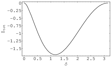
. We can finally collect all the results to obtain the maximal nonabelian contribution at order :
| (58) |
The plot for is given in fig. 14. We can easily perform a fit of the numerical result with a polynomial of the following form . This particular dependence is necessary in order to be in agreement with the conjectured relation with the zero-instanton sector of pure Yang-Mills theory on the sphere.

The coefficient is easily determined and it is . The difference between and the polynomial is less than over the whole range of the value of .
Thus we have
| (59) |
that exactly coincides with the second order expansion of the matrix model result (18), after the inclusion of the abelian contribution.
We have checked therefore the conjecture at two loops, at least for this particular class of loops. Now some remarks are in order: first of all we notice that in Feynman gauge double-exchange diagrams and the interactions conspire to reproduce the matrix model expression. This has to be contrasted with the circular Wilson loop case, where interactions vanish and simple exchange diagrams carry over the exact result. This suggests that probably there are more clever gauge choice to unveil the birth of the matrix model, may be contour-dependent. The second observation is that our formulae allow easily to perform explicit computations for other contours: all the integrals are in fact finite, and it is just matter of patience to put them on computer and evaluate them numerically. We remark again that in spite of the presence of the cusp, these supersymmetric Wilson loops are indeed finite.
5 Conclusions
In this paper we have studied at quantum level a family of supersymmetric Wilson loops in SYM which have been proposed in [41]. The contours are restricted to an submanifold of space-time and then for a curve of arbitrary shape a prescription for the scalar couplings guarantees that the resulting loop is globally supersymmetric. We have shown that no divergence arises in the perturbative expansion, also when non-smooth ”cusped” curves are considered and we derived a general compact representation for the contribution of interactions at order . Finally we presented a two-loop computation, supporting the evidence that this class of loops, that in general preserve four supercharges, may be described by a perturbative calculation in two-dimensional bosonic Yang-Mills theory on . We chose a “wedge” contour and we performed the necessary analytical and numerical evaluation to find consistency with the conjecture proposed in [41]. The agreement with the prediction of the matrix model, describing the zero-instanton sector of Yang-Mills theory on , is achieved in Feynman gauge after a non trivial conspiration of ladder and interacting diagrams: in this sense the situation here is quite different from the familiar circular Wilson loop, where exchange diagrams alone produce the correct matrix integral.
Many open questions remain of course to be answered: while our two-loop calculation points towards the validity of the correspondence between supersymmetric Wilson loops on and the gaussian matrix model of zero-instanton YM2, further checks, involving other contours and, may be, higher perturbative orders, are certainly welcome. More ambitiously one would like to generalize the localization approach on , elaborated in [40] for the circular loop, to the present situation, where a different amount of supersymmetry is preserved. In particular it would be important to understand the contributions of instantons in this case: instantons have been claimed to decouple in fact when the contour is a circle [40]. Another direction of work is to study, in this context, correlators of Wilson loops, to understand if the matrix model/two-dimensional Yang Mills description still holds: in the same spirit it would be also interesting to study the correlators with chiral primary operators, as done in [64] for a different class of loops. We end by observing that supersymmetry protects, in this case, cusped loops from being divergent: in a sense the BPS property smooths away the cusp anomalous behavior. It would be intriguing to understand better this last point and find, if any, connections among these exact results and the recent discovered perturbative properties of scattering amplitudes of SYM. All these directions are currently under investigations.
Acknowledgments
Two of us (DS and FP) would like thank to Galileo Galilei Institute for Theoretical Physics for hospitality during the completion of this work. DS and LG warmly thank N. Drukker for an illuminating discussion.
Appendices
Appendix A Light-cone analysis of planar Maldacena-Wilson loop
Contributions to the Wilson-loop at in light-cone gauge
In this Appendix we present an analysis of the contributions at to a space-like planar Maldacena-Wilson loop in light-cone gauge. We shall show that the diagrams are separately finite and no divergence arises from the integration over a smooth circuit.
Let us briefly recall some basic definitions and notations.
The light-cone gauge is characterized by the introduction of a light-cone vector leading to the gauge condition , being the vector potential (internal indices are understood). The free vector propagator in momentum space takes the form
being a null vector () such that . The usual choice is and . The first term in the propagator corresponds to its expression in Feynman gauge, whereas the second term is characteristic of the light-cone gauge.
Since the loop we are concerned with lies on the plane orthogonal to the gauge vectors, the contribution due to the exchange of two free propagators will not be different from the one in Feynman gauge and thereby will not be considered here.
The self-energy correction.
In ref.[63] the self-energy corrections to the gluon and scalar propagators at for SUSY have been computed. Since the Wilson loop we are considering lies on the plane orthogonal to the gauge vectors and , it is easy to convince oneself that only “transverse” Green functions contribute, which, in turn, get only corrections in this gauge [60], at variance with the more familiar Feynman gauge [26]. Since we expect that all the will be finite, there will be no need of a dimensional regularization. Typically in momentum space the gluon transverse Green function receives the correction
| (60) |
where , is the Euler’s dilogarithm and .
A direct calculation shows that the term containing the dilogarithm, when Fourier transformed and integrated over the contour, gives a vanishing contribution. Then the one-loop correction to the single exchange is
| (61) |
The triple vertex correction
The triple vertex diagram appears in the expansion of the Wilson-loop at the order . It corresponds to compute (we have suppressed a total factor , that will be inserted back at the end of the calculation)
| (62) |
where
| (63) |
and is defined in (29). Since the measure of integration is invariant under cyclic permutations, the integrand in (62) can simply be written as
| (64) |
To begin with, we shall compute
| (65) |
We have introduced the short-handed notation The tree-level correlation function is given in ref. [63]. We get
| (66) |
with . Then the contribution to the Wilson-loop is given by
| (67) |
where is the same function defined in sec. 3. Eq.(67) can be then cast in the form
| (68) |
which implicitly defines the functions and . Actually for a planar space-like Maldacena-Wilson loop the function can be rewritten in a way which is manifestly Lorentz invariant. Any reference to the original light-like directions disappears. The explicit expressions for and are given in appendix B.
Similarly, the scalar contribution turns out to be
| (69) |
where symmetry properties of the integrals have been suitably taken into account. Summing together vector and scalar contributions, we eventually obtain
| (70) |
This expression, a part from the kinematical factor, is identical to in (34). From here on we can follow exactly the same steps taken in sec. 3. We shall again find that cancels with a term coming from integrating by parts .
Eventually we are left with the gauge invariant result
| (71) |
We stress again that in light-cone gauge both self-energy correction and triple-vertex contribution are finite, at variance with what happens in Feynman gauge; there the two corrections exhibit a pole at and only in their sum the pole cancels and the finite quantity is eventually recovered.
It is almost trivial to realize that vanishes identically when the contour is a circle. Choosing the usual trigonometric parametrization for the circle, we can write
| (72) |
since the integrand
| (73) |
is antisymmetric under the exchange , while the measure and the region of integration are symmetric.
Appendix B Some properties of the integrals and
For the integral defined in (31) one can easily perform the integration over the momenta. In order to integrate over , we first introduce the Feynman parametrization for the two denominators, which depends on . Then we perform the change of variable . This yields
| (74) |
The integral over can be now evaluated by means of the Schwinger representation for the denominator in (74). We obtain
| (75) |
The integral over the second momentum can be now performed by introducing a second Schwinger parameter . We end up with the following parametric representation for
| (76) |
By setting , we can first integrate over and then over . In fact
| (77) |
In the last equality, we have used the following integral given on the table
| (78) |
This representation is useful to study the behavior around , and . Since (74) is manifestly symmetric in the exchange and , it is sufficient to study the behavior only around . The other two cases will obviously display a similar behavior. At we find
| (79) |
The integral is defined as follows
| (80) |
The origin of this object is explained in appendix A and it is related to light-cone gauge analysis of the Wilson-loop. There, its definition is given in momentum space. The expression (80) is obtained performing the integration over the momenta along the same path followed for .
In the following we shall compute its behavior at , and . At :
| (81) |
At :
| (82) |
At :
| (83) |
A useful combination of and :
In the following we shall show that the following combination of the derivatives of and ,
| (84) |
can be reduced to a very simple form. First, we shall take the derivative. We find
| (85) |
where
| (86) |
Since
| (87) |
the expression for can be rewritten as follows
| (88) |
The derivative of can be now computed by using the well-known properties of the hypergeometric functions:
| (89) |
where we have used the identity
| (90) |
Thus
| (91) |
References
- [1] J. M. Maldacena, Adv. Theor. Math. Phys. 2, 231 (1998) [Int. J. Theor. Phys. 38, 1113 (1999)] [arXiv: hep-th/9711200].
- [2] S. S. Gubser, I. R. Klebanov and A. M. Polyakov, Phys. Lett. B 428, 105 (1998) [arXiv: hep-th/9802109].
- [3] E. Witten, Adv. Theor. Math. Phys. 2, 253 (1998) [arXiv: hep-th/9802150].
- [4] J. A. Minahan and K. Zarembo, JHEP 0303, 013 (2003) [arXiv: hep-th/0212208].
- [5] N. Beisert, B. Eden and M. Staudacher, J. Stat. Mech. 0701, P021 (2007) [arXiv: hep-th/0610251].
- [6] Z. Bern, M. Czakon, L. J. Dixon, D. A. Kosower and V. A. Smirnov, Phys. Rev. D 75, 085010 (2007) [arXiv: hep-th/0610248].
- [7] M. K. Benna, S. Benvenuti, I. R. Klebanov and A. Scardicchio, Phys. Rev. Lett. 98, 131603 (2007) [arXiv: hep-th/0611135].
- [8] L. F. Alday, G. Arutyunov, M. K. Benna, B. Eden and I. R. Klebanov, JHEP 0704, 082 (2007) [arXiv: hep-th/0702028].
- [9] B. Basso, G. P. Korchemsky and J. Kotanski, Phys. Rev. Lett. 100, 091601 (2008) [arXiv: hep-th/0708.3933].
- [10] M. Beccaria, G. F. De Angelis and V. Forini, JHEP 0704, 066 (2007) [arXiv:hep-th/0703131].
- [11] I. Kostov, D. Serban and D. Volin, [arXiv: hep-th/0801.2542].
- [12] S. S. Gubser, I. R. Klebanov and A. M. Polyakov, Nucl. Phys. B 636, 99 (2002) [arXiv: hep-th/0204051].
- [13] S. Frolov and A. A. Tseytlin, Nucl. Phys. B 668, 77 (2003) [arXiv: hep-th/0304255].
- [14] R. Roiban, A. Tirziu and A. A. Tseytlin, JHEP 0707, 056 (2007) [arXiv: hep-th/0704.3638].
- [15] Z. Bern, L. J. Dixon and V. A. Smirnov, Phys. Rev. D 72, 085001 (2005) [arXiv: hep-th/0505205]
- [16] L. F. Alday and J. M. Maldacena, JHEP 0706, 064 (2007) [arXiv: hep-th/0705.0303].
- [17] J. M. Drummond, J. Henn, G. P. Korchemsky and E. Sokatchev, [arXiv: hep-th/0712.1223].
- [18] J. M. Drummond, J. Henn, G. P. Korchemsky and E. Sokatchev, Nucl. Phys. B 795, 52 (2008) [arXiv: hep-th/0709.2368].
- [19] J. M. Drummond, G. P. Korchemsky and E. Sokatchev, Nucl. Phys. B 795, 385 (2008) [arXiv: hep-th/0707.0243].
- [20] A. Brandhuber, P. Heslop and G. Travaglini, Nucl. Phys. B 794, 231 (2008) [arXiv: hep-th/0707.1153].
- [21] J. M. Drummond, J. Henn, G. P. Korchemsky and E. Sokatchev, [arXiv: hep-th/0712.4138].
- [22] Z. Bern, L. J. Dixon, D. A. Kosower, R. Roiban, M. Spradlin, C. Vergu and A. Volovich, [arXiv: hep-th/0803.1465].
- [23] J. M. Drummond, J. Henn, G. P. Korchemsky and E. Sokatchev, [arXiv: hep-th/0803.1466].
- [24] G. P. Korchemsky and A. V. Radyushkin, Nucl. Phys. B 283, 342 (1987).
- [25] G. P. Korchemsky and G. Marchesini, Nucl. Phys. B 406, 225 (1993) [arXiv: hep-ph/9210281].
- [26] J. K. Erickson, G. W. Semenoff and K. Zarembo, Nucl. Phys. B 582 (2000) 155 [arXiv: hep-th/0003055].
- [27] N. Drukker and D. J. Gross, J. Math. Phys. 42, 2896 (2001) [arXiv: hep-th/0010274]
- [28] N. Drukker and B. Fiol, JHEP 0502, 010 (2005) [arXiv: hep-th/0501109].
- [29] N. Drukker, S. Giombi, R. Ricci and D. Trancanelli, JHEP 0704, 008 (2007) [arXiv: hep-th/0612168].
- [30] S. Yamaguchi, JHEP 0605, 037 (2006) [arXiv: hep-th/0603208].
- [31] J. Gomis and F. Passerini, JHEP 0608, 074 (2006) [arXiv: hep-th/0604007].
- [32] J. Gomis and F. Passerini, JHEP 0701, 097 (2007) [arXiv: hep-th/0612022].
- [33] K. Okuyama and G. W. Semenoff, JHEP 0606, 057 (2006) [arXiv: hep-th/0604209].
- [34] S. A. Hartnoll and S. P. Kumar, JHEP 0608, 026 (2006) [arXiv: hep-th/0605027].
- [35] S. Giombi, R. Ricci and D. Trancanelli, JHEP 0610, 045 (2006) [arXiv: hep-th/0608077].
- [36] J. Plefka and M. Staudacher, JHEP 0109, 031 (2001) [arXiv: hep-th/0108182].
- [37] G. Arutyunov, J. Plefka and M. Staudacher, JHEP 0112, 014 (2001) [arXiv: hep-th/0111290].
- [38] G. Akemann and P. H. Damgaard, Phys. Lett. B 513, 179 (2001) [Erratum-ibid. B 524, 400 (2002)] [arXiv: hep-th/0101225].
- [39] C. Vafa and E. Witten, Nucl. Phys. B 431, 3 (1994) [arXiv: hep-th/9408074].
- [40] V. Pestun, [arXiv: hep-th/0712.2824].
- [41] N. Drukker, S. Giombi, R. Ricci and D. Trancanelli, [arXiv: hep-th/0711.3226].
- [42] E. Witten, J. Geom. Phys. 9, 303 (1992) [arXiv: hep-th/9204083].
- [43] D. Young, “BPS Wilson Loops on at Higher Loops,” arXiv:0804.4098 [hep-th].
- [44] S. J. Rey and J. T. Yee, Eur. Phys. J. C 22, 379 (2001) [arXiv: hep-th/9803001].
- [45] J. M. Maldacena, Phys. Rev. Lett. 80, 4859 (1998) [arXiv: hep-th/9803002].
- [46] M. Bianchi, M. B. Green and S. Kovacs, JHEP 0204, 040 (2002) [arXiv: hep-th/0202003].
- [47] K. Zarembo, Nucl. Phys. B 643, 157 (2002) [arXiv: hep-th/0205160].
- [48] Z. Guralnik and B. Kulik, JHEP 0401 (2004) 065 [arXiv: hep-th/0309118].
- [49] Z. Guralnik, S. Kovacs and B. Kulik, Int. J. Mod. Phys. A 20, 4546 (2005) [arXiv: hep-th/0409091].
- [50] A. Dymarsky, S. Gubser, Z. Guralnik and J. M. Maldacena, [arXiv: hep-th/0604058].
- [51] A. Kapustin and E. Witten, [arXiv: hep-th/0604151].
- [52] N. Drukker, D.J. Gross and H. Ooguri, Phys.Rev.D60:125006,1999, [arXiv: hep-th/9904191].
- [53] D. Berenstein, R. Corrado, W. Fischler and J. Maldacena, Phys. Rev. D59, 105023 (1999), [arXiv: hep-th/9809188].
- [54] A. Bassetto and L. Griguolo, Phys. Lett. B 443, 325 (1998) [arXiv: hep-th/9806037].
- [55] A. A. Migdal, Sov. Phys. JETP 42, 413 (1975) [Zh. Eksp. Teor. Fiz. 69, 810 (1975)].
- [56] V. A. Kazakov and I. K. Kostov, Nucl. Phys. B 176, 199 (1980).
- [57] B. E. Rusakov, Mod. Phys. Lett. A 5 (1990) 693.
- [58] M. Staudacher and W. Krauth, Phys. Rev. D 57, 2456 (1998) [hep-th/9709101].
- [59] T. T. Wu, Phys. Lett. B 71, 142 (1977).
- [60] S. Mandelstam, Nucl. Phys. B 213, 149 (1983).
- [61] G. Leibbrandt, Phys. Rev. D 29, 1699 (1984).
- [62] Y. Makeenko, P. Olesen and G. W. Semenoff, Nucl. Phys. B 748, 170 (2006) [arXiv: hep-th/0602100].
- [63] A. Bassetto and G. De Pol, Phys. Rev. D 77, 045001 (2008) [arXiv:hep-th/ 0705.4414].
- [64] G. W. Semenoff and D. Young, Phys. Lett. B 643, 195 (2006) [arXiv: hep-th/0609158].