Minimum-energy broadcast in random-grid ad-hoc networks: approximation and distributed algorithms Note: Research partially supported by the European Union under the Project AEOLUS
Abstract
The Min Energy Broadcast problem consists in assigning transmission ranges
to the nodes of an ad-hoc network in order to guarantee a
directed spanning tree from a given source node and, at the
same time, to minimize the energy consumption (i.e. the
energy cost) yielded by the range assignment.
Min Energy Broadcast is known to be NP-hard.
We consider random-grid
networks where nodes are chosen independently at random from
the points of a square grid in the
plane. The probability of the existence of a node at a given point
of the grid does depend on that point, that is, the probability
distribution can be non-uniform.
By using information-theoretic arguments, we
prove a lower bound
on
the energy cost of any feasible solution for this problem.
Then, we provide
an efficient solution of energy cost not larger than
.
Finally, we present a fully-distributed
protocol that constructs a broadcast range assignment of energy cost
not larger than ,
thus still yielding constant approximation.
The energy load is well balanced and, at the same time, the
work complexity (i.e. the energy due to all message
transmissions of the protocol)
is asymptotically optimal. The completion time of
the protocol is only an factor slower than the
optimum. The approximation quality of our distributed solution is also
experimentally evaluated.
All bounds hold with probability at least
.
1 Introduction
Range assignments in ad-hoc networks
In ad-hoc networks, nodes are able to vary their transmission ranges in order to provide good network connectivity and low energy consumption at the same time. More precisely, the transmission ranges determine a (directed) communication graph over the set of nodes: a node , with transmission range , can transmit to another node (so, edge ) if and only if belongs to the disk centered in and of radius . The transmission range of a node depends, in turn, on the energy power supplied to the node. In particular, the power required by a node to correctly transmit data to another station must satisfy the inequality , where is the Euclidean distance between and . In several works [2, 13, 18, 25], it is assumed that nodes can arbitrarily vary their transmission range over the ”large” set . However, in some important network scenarios (like sensor networks), this assumption is not realistic: the adopted technology allows nodes to have only few possible transmission range values. For this reason, we adopt the model considered in [10, 11, 17, 39] where nodes are able to choose their transmission range from a restricted set .
A fundamental class of algorithmic problems arising from
ad-hoc wireless networks consists in the range
assignment problems: find a transmission range assignment such that (1) the resulting communication
graph satisfies a given connectivity property , and (2) the
energy cost of the assignment is
minimized (see [18, 25]).
Several research works
[2, 13, 9, 18] have been devoted to the Min Energy Broadcast problem
where is defined as follows: Given a source node
, the communication graph has to contain a directed spanning
tree rooted at (a branching from ).
Previous theoretical results on Min Energy Broadcast concern
worst-case analysis only. This problem is known to be
NP-hard [13] even when
for and is set to any fixed positive constant.
The most famous approximation algorithm is the MST-based
heuristic [18]. This heuristics works in
time and its performance analysis has been the
subject of several works over the last years
[13, 19, 37]. In [2], it is finally proved
the tight bound 6 on its approximation ratio. More
recently, a new polynomial-time algorithm is provided in
[9] that achieves approximation ratio close to 4. This
algorithm applies a rather complex edge-contraction technique on
the MST-based solution. Its present best version works in
time and the design of any efficient distributed
version seems to be a very hard task.
It is important to observe that the MST-based heuristic is ”far” from achieving optimal solutions even on a complete square grid of points [6, 20]: its worst-case approximation ratio on such grids is not smaller than 3. In [20], it is also experimentally observed that this heuristic has a bad behavior when applied to random regular instances such as faulty square grids. Furthermore, the MST-based heuristic requires a large range set .
The above discussion leads us to study Min Energy Broadcast over random grid networks. Given a grid of points of the Euclidean plane (without loss of generality, adjacent points are placed at unit distance), each point11 1 For the sake of simplicity, we here assume that points are labelled with index . is selected as a node of the random grid network independently with probability . This node probability can be any value in the interval where and are two arbitrary positive constants in the interval . We remark that our random grids are in general non uniform: Random grids provide a good model for several ad-hoc and sensor networks. On one hand, by varying the ’s values, it is possible to model non homogenous input configurations with regions of different node densities. On the other hand, the grid structure guarantees a minimal distance among nodes: this is often a desired property in order to optimize area coverage and avoid message collisions. Nevertheless, as discussed later, all our results also hold for the standard uniform random distribution (i.e. the random input formed by choosing points independently and uniformly at random from a 2-dimensional square) [26, 34].
Our results
We
provide a lower bound on the energy cost of feasible solutions
for any range assignment problem on random grids where the
required property implies the existence of a
disk cover. We say that a range assignment is a
(disk) covering assignment if it guarantees that every node of
the network is within the positive range of some node.
Min Energy Broadcast is just one of those important cases requiring
covering range assignments.
Let be the minimum
positive range in
. For any , if
then
we prove that
the energy cost of any covering range assignment is with high
probability22
2
Here and in the sequel the term with high probability
means that the event holds with probability
at least for some constant . (in
short, w.h.p.)
at least . Observe that the
lower bound tends to for any such that
, so for minimal ranges much smaller
than
the connectivity threshold
[16, 23, 34, 35].
The proof’s technique of the lower bound departs
significantly from all those adopted in this topic and uses
information-theoretic arguments. By using this result, we will
prove that the next two algorithms are almost optimal.
We provide a simple and efficient algorithm for random grids that uses minimal range and returns a solution of energy cost not larger than w.h.p.: In virtue of our lower bound, this is very close to the optimum. Observe that our lower bound holds for any covering range assignment while the upper bound holds for feasible range assignments of Min Energy Broadcast: this implies that, for , the extra-cost, due to the required tree connectivity property, is ”almost” negligible in random grids (it is still an open problem whether this is in fact negligible). Our algorithmic solution works in time and needs a set of logarithmic size (in ). The range assignment is inspired to the one provided in [6] for complete square grids (i.e. every point of the grid is a node of the network). However, the probabilistic cost analysis of our construction for random grids is definitely not related to that in [6].
It is common opinion
that the development of
efficient, provably-good distributed algorithms is presently the major challenge about
range assignment problems [5, 37, 18].
We provide an efficient distributed algorithm
for Min Energy Broadcast on random grids. We investigate the performance of the protocol
in two different scenarios:
single broadcast and many-broadcast, i.e., a sequence
of consecutive broadcast operations.
In both cases, besides the energy cost of the returned range assignment,
we consider further important complexity aspects that determine the quality of a
distributed solution.
- Work Complexity.
In the ad-hoc network model, the work complexity of a distributed
algorithm (i.e. protocol)
for Min Energy Broadcast is defined as the sum of the energy cost
of all
transmissions made by the protocol to perform the broadcast
operation [24, 28, 36].
This complexity measure thus considers both the cost
to construct the range assignment and the cost to
use it to broadcast the message (the latter being
exactly the cost of the range assignment defined for centralized algorithms).
Since both the above energy costs are paid by the
nodes,
a protocol can be really considered energy efficient only if it has
a small work complexity.
- Energy-Load Balancing. In some real ad-hoc
networks (such as sensor networks), it is also important to equally distribute
the energy load to all nodes. For instance,
solutions, assigning large ranges to few nodes, are
not feasible in scenarios where nodes have limited
battery charges. In such a case, we aim to design
solutions that are well energy-load balanced.
Notice that, in the many-broadcast scenario, this
corresponds to maximize network lifetime according
to the model in [7, 8].
- (Amortized) Completion Time. Another relevant aspect of
a broadcast protocol is the completion time, i.e., the
number of time steps required to complete one
broadcast operation. In the many-broadcast scenario, the
amortized completion time is the average completion
time for one broadcast operation.
Our aim is to derive a protocol having
provably-good performance with respect to all the
above complexity aspects. To the best of our knowledge, no
available protocol has been shown to have
this overall performance.
We first define a very simple
range assignment where only one positive range in is
used, provided that it is not smaller than
where is a suitable positive constant (observe again that this value is asymptotically equivalent
to the connectivity threshold).
This
solution is then shown to be w.h.p. feasible and to have an energy
cost not larger than . Thanks to our lower bound, the achieved energy cost yields a constant
approximation ratio. Moreover, this simple range assignment can
be constructed and managed by an efficient
protocol. We assume every node
initially knows and its relative position with respect to the grid
only. Positioning information can be obtained
by using GPS systems or Ad-Hoc Positioning System (APS) [32].
This assumption is reasonable in
static ad-hoc networks since every node can
store once and for all its position in the set-up phase.
The protocol exploits a
fully-distributed pivot-election strategy borrowed from
[7].
We prove
that the work complexity of the protocol is
equivalent to the energy cost of the centralized version and
hence, thanks again to our lower bound
(clearly, a lower bound for the energy cost is also a lower bound for the work complexity), it achieves a constant
approximation ratio as well. It is important to emphasize that the
best distributed
algorithm to compute an MST
in the ad-hoc model has an
expected work complexity [22, 24, 29, 30]. By
comparing this bound with the work complexity achieved by our protocol, we can
state that any MST-based solution [18, 9] cannot yield
good work complexity in this scenario. Other distributed solutions have been
considered in the literature [5, 28, 36, 38], however their
performance analysis is based on experimental tests only.
We also compared the work complexity of our protocol to the energy cost
of the centralized MST-based solution over thousands of random instances with
different sizes and densities. The average performance ratio
between the two solutions is always between 2 and 3 (see Section
4.1) thus confirming our analytical results.
Our protocol yields a
good energy-load balanced solution: there are
pivots, i.e., the nodes having range (the remaining nodes have range 0). Furthermore, thanks to
the pivot-election strategy [7], a good energy-load
balance is also obtained with respect to an arbitrary sequence of broadcast
operations, i.e., for the many-broadcast scenario. At every new
operation, the pivot task is indeed assigned to nodes according to
a Round Robin rule. We show this yields an almost optimal
life-time of the network according to the energy
consumption model in [7, 8].
As for the single
broadcast scenario,
the completion time of our protocol is slower than the optimum
by a factor. As for the many-broadcast scenario,
when the number of broadcast operations
is , then the amortized completion time is
optimal.
Finally, we notice that, by using the technique in [31], our protocol can be emulated on the standard uniform random distribution [26, 34]. The same holds for the centralized algorithm achieving cost and for the lower bound as well. The relative proofs for the uniform distribution are easier and, so, they are omitted in this extended abstract.
Paper’s Organization
1.1 Preliminaries
The square grid of points will be indexed from to . Without loss of generality, the distance between adjacent points is set to 1. To each point of , a probability value is assigned such that where and are arbitrary constants in . We consider the random input model where an instance has probability
Observe that this probability distribution is equivalent to select each point independently with probability . A selected point will be called node. In the sequel, a subset selected according to the above random distribution will be simply called random set.
A set of disks is said to be an -cover for if the following properties hold: i) All disks of have radius at least , where is some positive value. ii) Every disk of has its center on a node of . iii) Every node of is covered by some disk of .
Observe that a range assignment can be represented by the family of disks yielded by the positive values of , and its energy cost is defined as
| (1) |
Furthermore, a feasible range assignment for the Min Energy Broadcast problem, with input and , uniquely determines an -cover for having the same cost. Notice that the converse is not true in general.
2 The lower bound
In this section, we provide a lower bound on the cost of any covering range assignment for a random set .
Definition 1
Let be the probability that a random set has an -cover of cost not larger than .
Theorem 2
Let and be three constants such that and . Let be any random set. Then, for any with , for sufficiently large , and for
it holds that
The above theorem clearly implies our lower bound stated in the Introduction and it requires no restriction about the transmission-range set but a lower bound on that does not depend on . In particular, if is any positive constant then, for sufficiently large grids and a sufficiently large constant (so does not depend on ), is not larger than the inverse of an exponential function in .
The theorem’s proof makes use of the following combinatorial result.
Lemma 3
Let be a partition of the points in and let be any -tuple of integers such that . Then, the number of subsets of such that () admitting an -cover with and is at most
where and
We now provide a brief description of the information-theoretic approach adopted to prove the above lemma.
Let be a subset of points of satisfying the hypothesis of the lemma. By exploiting the -cover , we will prove that can be encoded into a binary string of length at most
The lemma thus follows since the
number of these sets cannot exceed the number of binary
strings of the above length.
Proof of Lemma 3
Let be a subset of points of satisfying the hypothesis of the lemma. Consider the -cover of having the same centers of and where each radius in is replaced with a radius . Clearly, this change is negligible in terms of cost.
We now show that, thanks to , can be encoded into a binary string of length at most
Thus the thesis follows by noting that the number of these sets cannot exceed the number of binary strings of the above length.
The binary string encoding is the concatenation of four substrings , , and .
- a)
-
reports the number of centers of .
- b)
-
reports information to recover the indices of the nodes of that are centers in (we assume that the points in the grid are numbered from to ).
- c)
-
reports information to recover the radii of the nodes in .
- d)
-
reports information to recover the indices of the nodes in .
We now explain how these data are encoded and then bound the length of each of the four substrings.
- a)
-
The number of centers in is at most . Thus we encode it by a binary string of fixed length (i.e. ). Hence
(2) - b)
-
The centers of are a subset of the points in and so we encode them by a string of fixed length, i.e.
Since in the cover, each of the centers has radius at least , it must hold . From the hypothesis , we get
(3) As for substring , we obtain
Observe that in the above inequalities we used
since the function is increasing in the range ; then, from (3), is in the range .
- c)
-
Let now be the radii in arranged by increasing order of the indices of the centers. In order to give the information on the radii of , we encode string in binary where bit is encoded as , bit as and the symbol as . We thus get
(4) In the above inequalities, we first used since the product is maximized when all factors have the same value. Next, we used since the function is increasing in the range ; the value of is in the range ; and for . Finally, we bounded using (3).
- d)
-
In order to encode the nodes in , we use strings. The -th string encodes the points of in . The points of in covered by are a subset of the points in covered by . Hence, we encode these points with a binary string of length
Since for integers and where it holds that , we get
(5) where is the number of points of covered by . We now give an upper bound for .
Let be the number of points of covered by a disk of radius and, for each of these points, consider the square of area centered in the point. These squares are disjoint and are covered by the disk obtained by extending the radius of disk to . So, the number of points of covered by a disk of radius is bounded by . Moreover, it holds that
where the last inequality follows since . We thus obtain
Proof of Theorem 2
We assume
For any , with , define the binary function as follows
Clearly, it holds that
| (10) |
Let us partition into regions where such that for
Define as the expected number of points in , i.e., . Let be the family of subsets of having, in each region, a number of points not too small w.r.t. the expected number, i.e,
From (10) we get
| (11) |
We start giving an upper bound on the first addend of the right-hand of the above equation. Let
and, for each , define
Consider any set such that for every . Then,
| (12) |
where the last step follows from Lemma 3. Function is decreasing in and
We thus get
| (13) |
Assume without loss of generality that the points in are numbered in increasing order w.r.t. their probability i.e. . Let where , for . Consider any set , then
where
and
Function is decreasing for , so it holds that
Moreover, for every , it holds that . Thus, by setting and , we get
| (16) |
Function is increasing for and, by a simple calculus, we obtain
| (17) |
Moreover since
(15) implies
| (18) |
We now give an upper bound on the second addend in (11). Let , then
| (19) | |||||
3 An almost optimal solution
We now provide an efficient construction of a covering range assignment for a random set of energy cost very close to the lower bound . Then we will transform it, with additional cost only, into a feasible broadcast range assignment that uses ranges and such that the (positive) smallest among them, i.e. , is .
The disk covering construction
The construction of the covering is recursive and exploits a
tiling of the square with octagons and triangles.
The square of side is partitioned into
four triangles and an octagon (see Figure 1); up to
when there exists a triangle with side , it is
further on partitioned into five triangles (three small and two
big triangles) and an octagon (see Figure 2).


Starting from this partition, it is possible to produce a disk covering as follows (in the sequel, a range assignment is seen as a disk assignment with centers on nodes in ):
- •
for each triangle of the partition, if it contains at least one node, then one of them is selected as center of a disk having radius . Observe that this disk covers any other point inside the same triangle.
- •
for each octagon, if it contains at least one point that is not covered yet, then Lemma 5 implies that there is a node at distance to the center of the octagon, w.h.p. Let this node be the center of a disk having radius , where is the radius of the disk that circumscribes the considered octagon; the introduced disk covers all points in the octagon.
Theorem 4
Given a random set , then, w.h.p., disk covering has cost
Proof.
Let be the set of all the octagons in the partition, and for each call the radius of the disk that circumscribes octagon . Denoting by be the number of triangles in the partition, by construction it holds that:
| (20) |
Let be the side of the triangles created during the first step and let be the side of the first octagon (see Figure 1). The following equations hold: and . From these, we derive:
| (21) |
The recursive step depicted in Figure 2 produces triangles of two different sides and an octagon. Let and be the lengths of the sides of the bigger triangles, the smaller triangles and the octagon, respectively. These lengths are tied from the following relationships: , and , implying:
| (22) |
From (21) and (22), the triangles of the partition, generated during step , have side length , where and is the smallest integer value such that , i.e.,
| (23) |
Observe that all octagons (but the first one) of the partition are produced by partitioning some triangle of side length , . Denote by the radius of the disk that circumscribes the first octagon, by the radius of the disk that circumscribes the octagon produced by partitioning a triangle of side length , and by the number of such triangles. Then, we can rewrite (20) as follows:
| (24) |
We remind that the radius of the disk that circumscribes a regular octagon having side is . So, we can use (21) and (22) to compute the following values of and , respectively, where :
| (25) |
In order to compute the value of , observe that trivially (see Figure 1) and (see Figure 2). At step , . Unrolling the recursion we get:
| (26) |
In order to evaluate , we bound all terms appearing in (24) by exploiting (25) and (26):
| (27) | |||||
| (28) |
By combining Equations (26) and (23) we obtain:
| (29) | |||||
where the last step is true because . Furthermore,
| (30) |
Equation (26) implies that ; Then, from (29) we get:
| (31) |
By combining formulas (24), (27), (28), (30) and (31) we conclude that
From Covering to Broadcasting
In order to guarantee that the produced covering becomes a broadcast, we need to connect the source to the disk centers in . We start from the source, located in any place of the square, and build a chain of disks towards the center of the grid. Thanks to Lemma 5, the maximum radius of such disks can be bounded by , w.h.p. (see Fig. 3). We now show that the additional cost due to this construction turns out to be sub-linear.
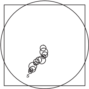
The cost of the connection between the source and the center of the square is w.h.p. Then we have to connect all the other centers to points already reached by the information sent from the source. The total cost due to this step is bounded by . By replacing the formulas for and we get:
This cost is sub-linear since it is . It is not hard to verify that the above overall construction can be performed in time.
4 An efficient distributed protocol
Let us consider the following simple algorithm to construct a broadcast range assignment. Let be any range in such that where is the constant determined by Lemma 5 below.
Algorithm cell-alg.
- a.
-
Grid is partitioned into square cells of side length .
- b.
-
In every non-empty cell, choose one of its nodes and assign range to it. This node is called the pivot of the cell.
- c.
-
The cell containing the source will have the source as pivot.
- d.
-
All other nodes have range 0.
The proof of the following lemma is a simple application of Chernoff’s Bound.
Lemma 5
Let , , and be three constants such that and . Let be a random grid. Consider the partition of into square cells of side length where . Then, a constant exists such that every cell contains w.h.p. at least nodes. Constant can be set as .
It is then easy to prove the following
Theorem 6
Algorithm cell-alg yields a broadcast range assignment that is w.h.p. feasible and its cost satisfies
Thanks to our lower bound in Theorem 2, cell-alg yields constant approximation.
Making it in distributed way
Algorithm cell-alg can be converted, without paying any extra energy cost, into an efficient, energy-load balanced protocol that performs a sequence of broadcast operations. We describe the protocol for the many-broadcast scenario and, thus, besides minimizing the energy spent by a single broadcast operation, we aim to evenly distribute the transmission task among all nodes (but the source).
According to the standard radio communication model
[3, 12, 27], we assume that nodes act in discrete
uniform time steps and are non spontaneous. However, we
assume a weaker, local synchronous model: if, at a given
time step , the range of a message transmission covers a cell,
then, at time step , (only) the nodes of that cell are
activated
and, so, they will agree on the same time step.
We assume that every node knows the number of points and its
relative coordinates in the square grid . From its relative
coordinates every node computes a unique local label with
respect to its cell. These local labels vary from to
.
The -th
message sent by the source is denoted as . Phase
consists of the sequence of time steps where is
broadcasted. We assume that
contains the value .
The protocol performs, in parallel, two tasks: i) it constructs a broadcast communication graph starting from the source and ii) transmits the source message along this graph to all nodes. The procedure is executed for every broadcast operation from source . Every node keeps a local counter counter initially set to .
Procedure Broadcast()
Source transmits, with range , where is the index of its cell.
All nodes (but ):
- •
If then ( is the constant of Lemma 5)
- –
When a node receives, for the first time w.r.t. phase , from the pivot of a neighbor cell , it becomes active.
- –
An active node, at every time step, increments its local counter counter by one and checks whether its local label is equal to the value of its counter. If this is the case, it becomes the pivot of its cell and transmits, with range , where is the index of its cell.
- –
When an active node in cell receives , it (so the pivot as well) records in a local array the current value of its counter, i.e. the local label of the pivot, and becomes inactive.
- –
- •
else (i.e. )
- –
When a node receives, for the first time w.r.t. phase , from the pivot of a neighbor cell , it checks if its local label is equal to . If this is the case, it becomes the pivot of its cell and transmits, with range , where is the index of its cell.
- –
Fact 7
Even though nodes initially do not know anything about each other, all nodes in the same cell are activated (and disactivated) at the same time step; so, their local counters share the same value at every time step. Furthermore, after the first broadcast operations (i.e. phases), all nodes in the same cell know the set of pivots of that cell.
More precisely, if are the local labels of the nodes in a cell, then, during the first broadcast operations (i.e. phases), the pivot of the cell at phase will be the node having local label .
Procedure Broadcast has the following properties.
Energy Cost. As for each single broadcast operation, Broadcast yields a broadcast range assignment equivalent to that of cell-alg. So, Theorem 6 holds as well.
Work Complexity.
Definition 8
Let be the set of all messages sent by the nodes according to a protocol . Then, the work complexity of is
The overall number of node transmissions (i.e. the
message complexity) of every execution of Broadcast is .
Each transmission has range , so the work complexity is not
larger than .
As for the many-broadcast scenario, our lower
bound in Theorem 2 easily implies that a work
is w.h.p. required to perform a sequence of
broadcasts (since the lower bound holds for the energy cost).
It follows that our protocol achieves an almost optimal work
complexity for the many-broadcast operation as well.
Load Balancing and Network Lifetime. The expensive pivot’s
task is evenly assigned, w.h.p., to
nodes (see Lemma
5) in the same cell by using a round robin
schedule.
This
is crucial when the number of broadcasts increases and nodes have limited battery charge.
As for the many-broadcast operation, it is possible to show that
our protocol achieves an almost maximal lifetime according to the
consumption model in [8, 7]. In this model,
the goal is to maximize the lifetime of the
network while
guaranteeing, at any phase , a broadcast operation from the source.
Formally, each node is initially equipped with a battery charge33
3
Here we assume that,
at the very beginning, all nodes
are in the same energy situation. . Whenever a node
transmits with range , its battery charge is
reduced by amount where
denotes the range assigned to node and is a fixed constant
depending on the adopted technology.
We assume , however, all our results holds for any
.
Then, the Max LifeTime problem is to maximize the
number of independent broadcast operations till some node will die
(i.e. its battery charge becomes 0).
In [8],
Max LifeTime is shown to be NP-hard.
Theorem 9
Broadcast performs a sequence of independent broadcast operations whose length is only a constant factor smaller than the optimum, w.h.p.
Sketch of proof. We have already observed that the work complexity
of Broadcast for any single broadcast operation is not larger than
, where is a positive constant and is
the optimal work complexity. So, the maximal number of
independent broadcast operations is not larger than .
Thanks to the local round robin strategy in every cell, the energy
load of the many-broadcast operation is well balanced over at
least a (large) constant fraction of all nodes. So the
number of broadcast operations perform by Broadcast is at least
,
w.h.p.
(Amortized) Completion Time.
Theorem 10
The amortized completion time (i.e. the average number of time steps to perform one broadcast operation) over a sequence of broadcast operations is w.h.p.
Sketch of proof. For a single broadcast operation performed by Broadcast, we define the delay of a cell as the number of time steps from its activation time till the selection of its pivot. Observe that the sum of delays introduced by a cell during the first broadcasts is at most . Then, the delay of any cell becomes 0 for all broadcasts after the first ones. Moreover, a broadcast can pass over at most cells. By assuming that a maximal length path (this length being together with maximal cell delay can be found in each of the first broadcasts, we can bound the maximal overall delay with
| (32) |
Finally, the number of time steps required by every broadcast without delays is
| (33) |
since the length of any path on the broadcast
tree is .
By combining
(32) and (33), we get the theorem bound.
For brevity’s sake, the amortized completion time has been analyzed without considering the interferences due to collisions among pivot transmissions [3]. However, in order to avoid such collisions, we can further organize Broadcast into iterative stages: in every stage, only cells with not colliding pivot transmissions are active. Since the number of cells that can interfere with a given cell is constant, this further scheduling will increase the overall time by a constant factor only. This iterative process can be efficiently performed in a distributed way since every node knows and its position, so it knows its cell.
Corollary 11
The completion time of one single broadcast operation is .
The worst scenario for our protocol occurs when is
small, say . Indeed, assume that a transmission range
is available in , then we get
an amortized completion time that is a
factor larger then the optimum. Notice that in this
case, the network
diameter is w.h.p.
Whenever , we instead get amortized completion
time which is optimal.
| vs | ||||||||
|---|---|---|---|---|---|---|---|---|
| # of feasible sol. | min | average | max | # of feasible sol. | min | average | max | |
| 13 | 744/1000 | 2.044 | 2.072 | 2.118 | 1000/1000 | 2.544 | 2.808 | 3.086 |
| 20 | 892/1000 | 1.896 | 2.092 | 2.145 | 999/1000 | 2.506 | 2.666 | 2.994 |
| 25 | 762/1000 | 2.040 | 2.127 | 2.164 | 998/1000 | 2.341 | 2.617 | 2.808 |
| 30 | 740/1000 | 2.163 | 2.217 | 2.242 | 997/1000 | 2.512 | 2.610 | 2.666 |
| 50 | 858/1000 | 2.313 | 2.398 | 2.450 | 999/1000 | 2.673 | 2.824 | 2.949 |
| 100 | 967/1000 | 2.300 | 2.347 | 2.352 | 1000/1000 | 2.604 | 2.659 | 2.702 |
4.1 Experimental results
In this subsection, we present the experimental results we have obtained by running Algorithm cell-alg. We have generated instances for every side length
and for node-probability . As usual, our implementation benefits of some parameter tuning and optimization: the pivot node (but the source node) inside every cell is the one closer to the center of the cell and useless, redundant ranges are removed. These tasks can be performed also by the distributed protocol, after the first phase (i.e. for ), without paying any extra energy cost since, after that time, every node of a cell knows all its cell neighbors. Moreover, the transmission range is set44 4 Notice that, for the tested sizes , this range is smaller than the threshold defined in Section 4: this is the reason why the feasibility rate is not 100% for large . to , while the cell-size parameter is set to . Notice that, according to such choices, the feasibility (i.e., the existence of a path from the source node to all other nodes in the induced communication graph) is tested too. In Table 1 (columns "# of feasible sol."), the number of feasible solutions for the different combinations of and are reported.
The solution costs of cell-alg are compared to the cost
of the solution returned by the centralized MST-based algorithm.
We remind that while the energy cost of cell-alg is an upper bound
on the work complexity of our distributed procedure Broadcast the
energy cost of the MST-based solution does not provide any
information about the work complexity of its distributed
implementations (this can be much larger).
Table 1 shows, for all chosen
values of and , the minimum, average and maximum
ratio between the costs of the solutions returned by the two
algorithms. As for cell-alg, only the costs of feasible
solutions are considered.
References
- [2] C. Ambuehl. An optimal bound for the MST algorithm to compute energy efficient broadcast trees in wireless networks. In Proc. of 32th ICALP, 1139–1150, 2005.
- [3] R. Bar-Yehuda, O. Goldreich, and A. Itai. On the time-complexity of broadcast in multi-hop radio networks: An exponential gap between determinism and randomization, JCSS, 45, 104-126, 1992.
- [4] R. Bar-Yehuda, A. Israeli, and A. Itai. Multiple communication in multi-hop radio networks, SICOMP, 22 (4), 875-887, 1993.
- [5] M. Cagali, J. Hubaux, and C. Enz. Minimum-energy broadcast in all-wireless networks: np-completeness and distribution issues. In Proc. of ACM MOBICOM, 172–182, 2002.
- [6] T. Calamoneri, A. Clementi, M. Di Ianni, M. Lauria, A. Monti, and R. Silvestri. Minimum Energy Broadcast and Disk Cover in Grid Wireless Networks. In Proc. of SIROCCO’06, LNCS, 2006.
- [7] T. Calamoneri, A. Clementi, E. Fusco and R. Silvestri. Maximizing the number of broadcast operations in static random geometric ad-hoc networks. In Proc. of OPODIS, LNCS, 2007.
- [8] G. Calinescu, S. Kapoor, A. Olshevsky, A. Zelikovsky. Network lifetime and power assignment in ad how wireless networks. In Proc. of ESA, LNCS, 2003.
- [9] I. Caragiannis, M. Flammini, and L. Moscardelli. An exponential improvement on the MST heuristic for the minimum energy broadcast problem. In Proc. of ICALP, LNCS, 2007.
- [10] M. Cardei and D-Z Du. Improving wireless sensor network lifetime through power organization. Wireless Networks, 11, 333–340, 2005.
- [11] M. Cardei, J. Wu, and M. Lu. Improving network lifetime using sensors with adjustable sensing ranges. Int. J. Sensor Networks, 1 (1/2), 41–49, 2006.
- [12] M. Chrobak, L. Gasieniec, and W. Rytter. Fast broadcasting and gossiping in radio networks, J. Algorithms, 43(2), 177–189, 2002.
- [13] A. Clementi, P. Crescenzi, P. Penna, G. Rossi and P. Vocca. On the Complexity of Computing Minimum Energy Consumption Broadcast Subgraphs. In Proc. of 18th STACS, LNCS 2010, 121–131, 2001. Full version in http://www.dia.unisa.it/penna/no-blood-for-oil.html.
- [14] A. Clementi, P. Penna, and R. Silvestri. On the Power Assignment Problem in Radio Networks. ACM Mobile Networks and Applications (MONET), 9, 125–140, 2004.
- [15] P. Crescenzi and V. Kann, A Compendium of NP Optimization Problems. http://www.nada.kth.se/viggo/wwwcompendium/.
- [16] A. Dessmark and A. Pelc. Broadcasting in geometric radio networks. Journal of Discrete Algorithms, 2006.
- [17] O. Egecioglu and T. Gonzalez. Minimum-energy broadcast in simple graphs with limited node power. In Proc. of IASTED PDCS, 2001.
- [18] A. Ephremides, G.D. Nguyen, and J.E. Wieselthier. On the Construction of Energy-Efficient Broadcast and Multicast Trees in Wireless Networks. In Proc. of 19th IEEE INFOCOM, 585–594, 2000.
- [19] M.Flammini, R.Klasing, A.Navarra, S.Perennes. Improved Approximation Results for the Minimum Energy Broadcasting Problem, Algorithmica, 49(4), 318–336, 2007.
- [20] M. Flammini, A. Navarra, and S. Perennes. The Real Approximation Factor of the MST Heuristic for the Minimum Energy Broadcast. In Proc. of WEA, 22–31, 2005.
- [21] A. D. Flaxman, A. M. Frieze, and J. C. Vera. On the average case performance of some greedy approximation algorithms for the uncapacitated facility location problem. In Proc. of 37-th ACM STOC, 441–449, 2005.
- [22] R. Gallager, P. Humblet, and P. Spira. A distributed algorithm for minimum spanning tree. ACM Trans. on Progr. Languages and Systems, 5 (1), 66–77, 1983.
- [23] P. Gupta and P.R. Kumar. Critical power for asymptotic connectivity in wireless networks. In Stochastic Analysis, Control, Optimization and Applications. Birkhauser, 547–566, 1999.
- [24] M. Khan, G. Pandurangan, and V.S.A. Kumar. Distributed Algorithms for Constructing Approximate Minimum Spanning Trees in Wireless Sensor Networks. IEEE Transactions on Parallel and Distributed Systems, 2008, to appear.
- [25] L. M. Kirousis, E. Kranakis, and D. Krizanc, and A. Pelc. Power Consumption in Packet Radio Networks. Theoretical Computer Science, 243, 289–305, 2000.
- [26] G. Kozma, Z. Lotker, M. Sharir, and G. Stupp. Geometrically aware communication in random wireless networks. In Proc. of 23rd ACM PODC, 2004.
- [27] E. Kranakis, D. Krizanc, and A. Pelc. Fault-tolerant broadcasting in radio networks. Journal of Algorithms, 39, 47–67, 2001.
- [28] X. Li, G. Calinescu and P. Wan. Distributed construction of planar spanner and routing for ad hoc wireless networks. Proc. of INFOCOM, 2002.
- [29] X. Li. Localized construction of low weighted structures and its applications in in wireless ad-hoc networks. ACM Wireless Networks, 2003.
- [30] X. Li, Y. Wang, W. Song, and O. Frieder. Localized low-weight graph and its applications in wireless ad-hoc networks. In Proc. of IEEE INFOCOM, 2004.
- [31] Z. Lotker and A. Navarra. Managing Random Sensor Networks by means of Grid Emulation. In Proc. of NETWORKING, LNCS 3976, 2006.
- [32] D. Niculescu and B. Nath. Ad-Hoc Positioning System (APS). In Proc. of IEEE GLOBECOM, 2001.
- [33] K. Pahlavan and A. Levesque. Wireless Information Networks. Wiley-Interscience, 1995.
- [34] M. Penrose. Random Geometric Graphs. Oxford University Press, 2003.
- [35] P. Santi and D. M. Blough. The Critical Transmitting Range for Connectivity in Sparse Wireless Ad Hoc Networks IEEE Trans. on Mobile Computing, 2: 25-39, 2003.
- [36] R. Ramanathan and R. Rosales-Hain. Topology control of multihop wireless networks using transmit power adjustment. In Proc. of IEEE-INFOCOM, 2000.
- [37] G. Calinescu, X.Y. Li, O. Frieder, and P.J. Wan. Minimum-Energy Broadcast Routing in Static Ad Hoc Wireless Networks. In Proc. of 20th IEEE INFOCOM, 1162–1171, April 2001.
- [38] Y. Wang, X. Li, and O. Frieder. Distributed Spanner with bounded degree for wireless ad hoc networks. IEEE Trans. on Computers, 53(12): 1629–1635, 2004.
- [39] J. Wu and S. Yang. Coverage and connectivity in sensor networks with adjustable ranges. Proc. of Intern. Workshop on Mobile and Wireless Networking (MWN), 2004.