Transonic and subsonic flows in general relativistic radiation hydrodynamics

Consider a general-relativistic system — a compact core immersed in a steadily accreting selfgravitating gas. The gravitational binding energy of the infalling gas can be converted to a radiation. Assume that an external distant observer can measure total luminosity, asymptotic temperature and redshifts of the radiation. Let be known: the total (asymptotic) mass of the system and the physics of the mixture of gas and radiation. Then it would be natural to ask: what mass is within the compact body? Alternatively, the mass of the core would be known and the total mass would require determination.

The main goal of this paper is the numerical investigation of this problem for stationary flows. We assume spherical symmetry and adopt thin gas approximation in the transport equation. It is already known from studies of newtonian radiation hydrodynamics [1] — [3] that supersonic flows are generically not fixed by total luminosity, asymptotic temperature and redshift. To each set of such data there can correspond two solutions with different gas abundances. Changing luminosity one obtains two curves, on the luminosity-(gas abundance) diagram, that originate at a bifurcation point. This point is unique, for given boundary data. General-relativistic supersonic flows with small redshifts are similar to newtonian ones in that they also branch from a bifurcation transonic flow. In the case of high redshifts supersonic general-relativistic flows can be absent. A similar picture appears in transonic flows of perfect gases, newtonian or general-relativistic, without radiation. In this case boundary data can consist of the mass accretion rate and the asymptotic speed of sound [4] and the only unique solution — a branching point — corresponds to the maximal accretion.

Accretion systems with subsonic flows are not determined by the data described hitherto. One needs additional information, for instance the asymptotic gas density, in order the specify the solution completely. We discover, however, an interesting fact valid in the newtonian case and in the low-redshift regime of general relativity: transonic flows encompass, on the luminosity-(gas abundance) diagram, the set filled with subsonic flows. Therefore the two transonic branches provide estimates of the mass abundance of corresponding subsonic solutions. In particular, numerical analysis suggests that the most luminous flow is supersonic. This picture is valid in the newtonian level and also in the general-relativistic case, for small redshifts. If redshifts are large, then the boundary of the set of subsonic solutions may consist of transonicor subsonic flows, but it is remarkable that the shape of the set of subsonic solutions is only weakly dependent on redshifts. In particular, the flow with maximal luminosity is unique.

This investigation can be useful in the analysis of two important issues. There is the question of identification of the so-called Thorne-Żytkow stars [5], that consist of a hard core and overblown atmosphere. They are conjectured to result in the merger of a main sequence star with a neutron star or a black hole. If the core consists of a neutron star, then its mass is roughly known. Results of this paper show that one can estimate the total mass by measuring luminosity, asymptotic temperature and redshifts. Another interesting application would be to distinguish compact stars (neutron stars or gravastars [6]) from black holes, but the present analysis would require further elaboration. Within the scenario investigated here it does not seem feasible to distinguish between a black hole or a gravastar, but the investigation of stability can possibly give further information.

The organization of the rest of this paper is following. Section 2 presents spherically symmetric equations of radiation hydrodynamics. The next section explains the concept of quasistationary solutions. The interaction of gas and radiation is treated in the thin gas approximation [7]. The final form of required equations is displayed. Boundary conditions are described in Section 4. The next Section brings a discussion of boundary conditions. In particular, we explain the relation between the binding energy of collapsing fluids and radiation redshifts. We demonstrate in Section 6 that supersonic solutions constitute a one-sided boundary for the set of subsonic solutions in newtonian test fluids. Section 7 shows main results of this paper — relations between transonic and subsonic flows in the general-relativistic case. The last section contains a summary.

We use comoving coordinates $t,r,0\leq\theta\leq\pi,0\leq\phi<2\pi$: time, coordinate radius and two angle variables, respectively. The metric can be chosen in the form

$$ds^{2}=-N^{2}dt^{2}+\tilde{a}dr^{2}+R^{2}d\Omega^{2}.$$

(1)

$R$ in (1) is the area radius. The infall velocity of gas is equal to $U=\frac{1}{N}\frac{dR}{dt}$ and it is related to extrinsic curvatures of the Cauchy hypersurface $t=\mathrm{const}$,

$$\left(\mathop{\mathrm{tr}}K-K^{r}_{r}\right)R=2U.$$

(2)

$\mathop{\mathrm{tr}}K$ is the trace of the extrinsic curvature and $K_{r}^{r}$ is its radial-radial component.

The energy-momentum tensor reads $T_{\mu\nu}=T_{\mu\nu}^{B}+T_{\mu\nu}^{E}$, where the baryonic part is given by $T_{\mu\nu}^{B}=(\rho+p)U_{\mu}U_{\nu}+pg_{\mu\nu}$ with the time-like and normalized four-velocity $U_{\mu}$, $U_{\mu}U^{\mu}=-1$. The radiation part has only four nonzero components, $T_{0}^{0E}\equiv-\rho_{E}=-T_{r}^{rE}$ and $T^{E}_{r0}=T^{E}_{0r}$, which is consistent with the so-called thin gas approximation (see next section).

A comoving observer would measure local mass densities, material $\rho=T^{B\mu\nu}U_{\mu}U_{\nu}$ and radiation $\rho_{E}$, respectively. The baryonic current is defined as $j^{\mu}\equiv\rho_{0}U^{\mu}$, where $\rho_{0}$ is the baryonic mass density. Define $n_{\mu}$ as the unit normal to a centered (coordinate) sphere lying in the hypersurface $t=\mathrm{const}$ and $k$ as the related mean curvature scalar, $k={R\over 2}\nabla_{i}n^{i}=\frac{1}{\sqrt{\tilde{a}}}\partial_{r}R$. The comoving radiation flux density reads $j=U_{\mu}n^{\nu}NT^{\mu E}_{\nu}/\sqrt{\tilde{a}}=NT^{0E}_{r}/\sqrt{\tilde{a}}$.

We assume a polytropic equation of state for the baryonic matter, $p=K\rho_{0}^{\Gamma}$ ($K$ and $\Gamma$ are constants) and the relation

$$\rho=\rho_{0}+h,$$

(3)

where the internal energy $h$ is easily shown to be equal to $p/(\Gamma-1)$. The equations of motion consist, in the spherically symmetric case, of three Einstein equations, of two constraints [8]

$$\frac{1}{R}\partial_{R}\left(Rk^{2}\right)=-R\Bigl(8\pi\left(\rho+\rho_{E}\right)+\frac{3}{4}(K_{r}^{r})^{2}\Bigr)+\frac{1}{R}+\frac{R}{4}(\mathop{\mathrm{tr}}K)^{2}+\frac{R}{2}\mathop{\mathrm{tr}}KK_{r}^{r},$$

(4)

$$\frac{\partial_{r}(K_{r}^{r}-\mathop{\mathrm{tr}}K)}{\sqrt{\tilde{a}}}=-\frac{3}{R}kK_{r}^{r}-8\pi j+\frac{1}{R}k\mathop{\mathrm{tr}}K,$$

(5)

and one dynamical equation

	$\displaystyle\partial_{t}(K_{r}^{r}-\mathop{\mathrm{tr}}K)=\frac{3N}{4}(K_{r}^{r})^{2}-\frac{Nk^{2}}{R^{2}}-\frac{2k}{R\sqrt{\tilde{a}}}\partial_{r}N+\frac{N}{R^{2}}$				(6)
			$\displaystyle+8\pi NT_{r}^{r}+\frac{3}{4}N(\mathop{\mathrm{tr}}K)^{2}-\frac{3N}{2}\mathop{\mathrm{tr}}KK_{r}^{r}.$

The baryonic current is conserved,

$$\nabla_{\mu}j^{\mu}=0.$$

(7)

There are four conservation equations $\nabla_{\mu}T^{\mu B}_{\nu}=-\nabla_{\mu}T^{\mu E}_{\nu}={\mathcal{F}}_{\nu}$ (here $\nu=0,r$). The quantity ${\mathcal{F}}_{\nu}$ is called the radiation force density and it describes interaction between baryons and radiation. Its radial component will be written as ${\mathcal{F}}_{r}\equiv k\sqrt{\tilde{a}}F_{r}$; $F_{r}$ is defined later. The formulation of general-relativistic radiation hydrodynamics presented here agrees with that of Park [9] and Miller and Rezzola [10], and (on a Schwarzschildean background) with Thorne et. al [11]. One can solve formally both constraints, arriving at [8]

	$\displaystyle k=\sqrt{1-\frac{2m(R)}{R}+U^{2}},$
	$\displaystyle K_{r}^{r}=\partial_{R}U-4\pi R\frac{j}{k},$
	$\displaystyle\mathop{\mathrm{tr}}K={1\over R^{2}}\partial_{R}\left(UR^{2}\right)-4\pi R\frac{j}{k}.$		(8)

Here $m(R)$ is the quasilocal mass

$$m(R)=m(R_{\infty})-4\pi\int_{R}^{R_{\infty}}drr^{2}\left(\rho+\rho_{E}+\frac{Uj}{k}\right).$$

(9)

The integration in (9) extends from $R$ to the outer boundary $R_{\infty}$ of the accretion system. $m(R_{\infty})$ can be equal (or arbitrarily close) to the total asymptotic mass $M$. The contribution to the mass coming from the exterior of $R_{\infty}$ can be neglected. Comoving coordinates can be understood as a choice of a particular integral-type gauge condition [12]. In what follows we will use the comoving spacetime foliations, with the time $t$ but often with the areal radius $R$ instead of the comoving radius $r$. The parametrization ($t$, $R$) can be interpreted as corresponding to an observer at rest at $R$.

One can choose an alternative set of coordinates in a different spacetime foliation, in the so-called polar gauge $\mathop{\mathrm{tr}}K=K_{r}^{r}$ (no summation), with the time $t_{S}=t_{S}(R,t)$ and the areal variable $R$. We do not employ these variables here (but see a remark below).

A simple but lengthy calculation shows that the local mass changes according to the following rule

$$\partial_{t_{S}}m(R)=\left(\partial_{t}-NU\partial_{R}\right)m(R)=4\pi\left(NkR^{2}\left(j\left(1+\left(\frac{U}{k}\right)^{2}\right)+2\rho_{E}{U\over k}\right)+NUR^{2}\left(\rho+p\right)\right)_{R}^{R_{\infty}}+A_{\infty},$$

(10)

where $A_{\infty}$ is the value of $-4\pi NUR^{2}\left(\rho+\rho_{E}+\frac{Uj}{k}\right)$ at $R=R_{\infty}$. It is interesting to note that the expression $4\pi NkR^{2}\left(j\left(1+\left(\frac{U}{k}\right)^{2}\right)+2U\rho_{E}/k\right)$ represents the radiation flux measured by an observer located at $R$ in the polar gauge foliation. The mass contained in the annulus $(R,R_{\infty})$ changes if the fluxes on the right hand side do not cancel. In the case of quasistationary flows the mass is approximately constant.

We will say that the accretion process is quasistationary if all relevant quantities measured in the rest frame are approximately constant during time intervals much smaller than certain characteristic time scale $T$. In analytical terms, we assume that $\partial_{t_{S}}X=(\partial_{t}-NU\partial_{R})X=0$ for $X=\rho_{0}$, $\rho$, $j$, $U$…

Under quasistationarity assumption the evolution equation (6) can be written as

$$U\frac{dU}{dR}=\frac{k^{2}}{N}\frac{dN}{dR}-\frac{m(R)}{R^{2}}-4\pi R\left(p+\rho_{E}\right)$$

(11)

From this one easily obtains

$$N=k\exp\left(-4\pi\int_{R}^{R_{\infty}}dr\frac{r}{k^{2}}\left(\rho+p+2\rho_{E}+\frac{Uj}{k}\right)\right).$$

(12)

The local accretion mass rate ${\dot{M}}$ is defined as

$${\dot{M}}\equiv-4\pi UR^{2}\rho_{0}.$$

(13)

The baryonic current conservation equation (7) takes the form $\partial_{R}{\dot{M}}=-16\pi^{2}jR^{3}\frac{\rho_{0}}{k}$; thus the local mass accretion rate ${\dot{M}}$ can change, but the quantity

$$\tilde{M}\equiv-4\pi UR^{2}\rho_{0}-(4\pi)^{2}\int_{R}^{R_{\infty}}drr^{3}j\frac{\rho_{0}}{k}$$

(14)

remains constant, $\frac{d}{dR}\tilde{M}=0$. Notice that ${\dot{M}}\left(R_{\infty}\right)=\tilde{M}$.

As the characteristic time scale one can choose the quantity related to the runaway instability, $T\equiv M/\tilde{M}$. One can obtain a rough estimate $\frac{d}{dt}\tilde{M}\leq CM^{2}$ where $C$ is a constant (see [1] for the corresponding derivation in the newtonian case). Let $M_{0}$ be the initial mass. Then $M\leq 1/\left(1-CM_{0}t\right)$. If $M/\tilde{M}\gg t$ then $M\approx M_{0}$ and if $t\approx T$ then $M\gg M_{0}$; thus the time $T$ sets the time scale for the runaway instability.

The radiation force density has only one nonzero component. It is a simple exercise to show that the conservation of $\tilde{M}$ and relation (3) imply, for polytropic gases, the vanishing of the zeroth component of the radiation force, ${\mathcal{F}}_{0}$. Therefore the two related energy and radiation energy balance equations read

	$\displaystyle NU\frac{d\rho}{dR}+N\mathop{\mathrm{tr}}K\left(p+\rho\right)$	$\displaystyle=$	$\displaystyle 0$
	$\displaystyle\frac{N}{UR^{2}}\frac{d}{dR}\left(U^{2}R^{2}\rho_{E}\right)+\frac{k}{R^{2}N}\frac{d}{dR}\left(N^{2}R^{2}j\right)-8\pi NRj\frac{\rho_{E}}{k}$	$\displaystyle=$	$\displaystyle 0.$		(15)

The two other energy-momentum conservation equations are displayed below. The relativistic Euler equation is given by

$$\frac{1}{N}\frac{dN}{dR}\left(p+\rho\right)+\frac{dp}{dR}=F_{r}$$

(16)

and the transport equation reads

$$\frac{N}{UR^{2}}\frac{d}{dR}\left(U^{2}R^{2}j\right)+\frac{k}{R^{2}N}\frac{d}{dR}\left(N^{2}R^{2}\rho_{E}\right)-8\pi Rj^{2}\frac{N}{k}=-NkF_{r}.$$

(17)

There enters an important phenomenological assumption that can be easily expressed in terms of quantities related with comoving coordinates. Namely we assume the so-called thin gas approximation [7]

$$F_{r}=\kappa\rho_{0}j.$$

(18)

The only direct interaction between baryons and radiation is through elastic Thompson scattering. $\kappa$ is a material constant, depending in particular on the Thompson cross section $\sigma$, $\kappa=\sigma/\left(4\pi m_{p}c\right)$. $c$ is the speed of light and $m_{p}$ is the proton mass.

In summary, the complete set of equations would consist of eqs (8), (9) and (12–18).

It is convenient to express all relevant quantities in terms of the speed of sound $a$, given by $a^{2}\equiv{dp\over d\rho}$, because we will search for flows possessing transonic points. We find that it is computationally expedient to replace the radiation energy balance equation (the second of eqs (15)) by the total energy conservation

$${\dot{M}}N\frac{\Gamma-1}{\Gamma-1-a^{2}}+2{\dot{M}}N\frac{\rho_{E}}{\rho_{0}}=4\pi R^{2}jNk\left(1+\frac{U^{2}}{k^{2}}\right)+C.$$

(19)

Equation (19) is a direct consequence of quasistationarity and the equation (10). The constant $C$ is the asymptotic flux (i.e., flowing through the sphere of a radius $R_{\infty}$) in (10).

Furthermore, write down eq. (17) as

	$\displaystyle\frac{NU}{R^{2}}\frac{d}{dR}\left(R^{2}j\right)=-\kappa kNj\rho_{0}-\frac{kN}{R^{2}}\frac{d}{dR}\left(R^{2}\rho_{E}\right)-$				(20)
			$\displaystyle 2Nj\frac{dU}{dR}-2k\rho_{E}\frac{dN}{dR}+8\pi NR\frac{j^{2}}{k}.$

and replace the term $\frac{NU}{R^{2}}\frac{d}{dR}\left(R^{2}j\right)$ in the second of equations (15). After some algebra one arrives at

	$\displaystyle\left(1-\frac{2m(R)}{R}\right)\frac{N}{R^{2}}\frac{d}{dR}\left(R^{2}\rho_{E}\right)=-\kappa k^{2}Nj\rho_{0}+2N\left(U\rho_{E}-kj\right)\frac{dU}{dR}+$				(21)
			$\displaystyle 2k\left(jU-k\rho_{E}\right)\frac{dN}{dR}+8\pi NR\left(j^{2}-j\rho_{E}\frac{U}{k}\right).$

Below we display a number of relations, that can be easily obtained from the equation of state and (3), namely

	$\displaystyle\frac{p}{\rho_{0}}$	$\displaystyle=$	$\displaystyle\frac{\Gamma-1}{\Gamma}\frac{a^{2}}{\Gamma-1-a^{2}},$
	$\displaystyle\frac{p+\rho}{\rho_{0}}$	$\displaystyle=$	$\displaystyle\frac{\Gamma-1}{\Gamma-1-a^{2}},$
	$\displaystyle\frac{\partial_{R}p}{p+\rho}$	$\displaystyle=$	$\displaystyle\partial_{R}\ln\left(\frac{\rho+p}{\rho_{0}}\right)=-\partial_{R}\ln\left(\Gamma-1-a^{2}\right),$
	$\displaystyle\rho_{0}$	$\displaystyle=$	$\displaystyle\rho_{0\infty}\left(\frac{a}{a_{\infty}}\right)^{\frac{2}{\Gamma-1}}{\left(1-\frac{a^{2}_{\infty}}{\Gamma-1}\right)^{\frac{1}{\Gamma-1}}\over\left(1-\frac{a^{2}}{\Gamma-1}\right)^{\frac{1}{\Gamma-1}}}.$		(22)

It is useful to insert (22) into Eqs. (14—18). One obtains following equations:

1. i)

   the gas energy density conservation equation (the first of eqs. (15))

   	$\displaystyle\frac{d}{dR}\ln a^{2}=-\frac{\Gamma-1-a^{2}}{a^{2}-\frac{U^{2}}{k^{2}}}\times$				(23)
   			$\displaystyle\Biggl(\frac{1}{k^{2}R}\left(\frac{m}{R}-2U^{2}+4\pi R^{2}\left(\rho_{E}+p+j\frac{U}{k}\right)\right)-$
   			$\displaystyle\kappa j\left(1-\frac{a^{2}}{\Gamma-1}\right)\Biggr);$

2. ii)

   the baryonic mass conservation

   $$\frac{dU}{dR}=-\frac{U}{\Gamma-1-a^{2}}\frac{d}{dR}\ln a^{2}-\frac{2U}{R}+\frac{4\pi Rj}{k};$$

   (24)

3. iii)

   the equation for the lapse

   $$\frac{dN}{dR}=N\left(\kappa j\frac{\Gamma-1-a^{2}}{\Gamma-1}+\frac{d}{dR}\ln\left(\Gamma-1-a^{2}\right)\right).$$

   (25)

   Eq. (25) follows from (16) and (22).

Equations (19), (21) and (23—25) constitute, with $k$ and $m(R)$ given by (8) and (9), the complete model used in numerical calculations reported in next sections. A remark is in order. It is clear from the inspection of (23) that if $a^{2}=\frac{U^{2}}{k^{2}}$ (the speed of sound equals the spatial length of the infall velocity) then the expression $\frac{1}{k^{2}R}\left(\frac{m}{R}-2U^{2}+4\pi R^{2}\left(\rho_{E}+p+j\frac{U}{k}\right)\right)-\kappa j\left(1-\frac{a^{2}}{\Gamma-1}\right)$ must vanish. There are four different ways of passing through the transonic point (similarly as in the newtonian analysis in [13]) and only one of those corresponds to the accretion.

The overall picture of the system is as follows. A ball of gas is enclosed by a sphere $S_{\infty}$ of a radius $R_{\infty}$ and connected, via a narrow transient zone filled with baryonic matter and radiation, to the Schwarzschild vacuum spacetime. It is clear that by careful arrangement of data the mass within the transient zone can be negligible. Therefore we assume that the asymptotic mass $M$ is equal to $m\left(R_{\infty}\right)$ (see Eq. (9)).

Boundary conditions at the outer sphere $S_{\infty}$ are needed for the radiation quantities $j$, $\rho_{E}$, the mass accretion rate ${\dot{M}}$, the square of the speed of sound $a^{2}_{\infty}$ and the baryonic mass $\rho_{\infty}$. We assume that $a^{2}_{\infty}\gg M/R_{\infty}\gg U^{2}_{\infty}$; the second inequality means that infall velocity is much smaller than the escape velocity. These inequalities guarantee the fulfillment of the Jeans criterion for the stability (see a discussion in [1] and studies of stability of accreting flows in newtonian hydrodynamics [17]), suggesting the stability of solutions.

One can derive, after some algebra involving manipulations of equations (20) and (21), the approximate equation $\frac{d}{dR}\left(\left(\rho_{E}-j\right)R^{2}\right)\approx 0$ in the asymptotic region. This means, taking into account the fact that $R_{\infty}$ can be arbitrarily large, that one can safely assume $j_{\infty}=\rho_{E_{\infty}}$. Furthermore, the total luminosity is with good accuracy given by $L_{0}=4\pi R^{2}_{\infty}j_{\infty}$ and it must be related to the accretion rate by the formula

$$L_{0}\equiv\alpha{\dot{M}}_{\infty}.$$

(26)

The coefficient $\alpha$ determines the relative binding energy. We assume

$$\alpha\equiv 1-\frac{N\left(R_{0}\right)}{k\left(R_{0}\right)}\sqrt{1-\frac{2m\left(R_{0}\right)}{R_{0}}},$$

(27)

where $R_{0}$ is the outer radius of the hard core of the system. The last two formulae can be justified by two arguments. First, in the nonrelativistic limit one gets $\alpha=|\phi\left(R_{0}\right)|$; $\alpha$ is equal to the absolute value of the newtonian potential on the surface of the hard body. It is clear now that (26) is just the statement that all available binding energy is transformed into radiation, and that there is an implicit assumption that the heat capacity of the core is negligible. Second, the condition of stationarity implies the existence of the approximate time-like Killing vector. By employing standard reasoning [18], one arrives at the two formulae (26) and (27). Thus $\alpha$ can be regarded as a proper binding energy. Let us remark that $\alpha$ gives the standard measure of the gravitational red- or blue-shift. If stationary observers detect $\omega_{0}$ at $R_{0}$ and $\omega$ at infinity, and $1/\omega\ll 2M$ (the geometric optics condition — see [19] for a discussion) then $\omega=\left(1-\alpha\right)\omega_{0}$.

In conclusion, boundary data consist of the binding energy coefficient $\alpha$, total luminosity $L_{0}$ and the asymptotic speed of sound $a^{2}_{\infty}$. Not only $L_{0}$ but also the two remaining quantities can be in principle determined from observations: $\alpha$ from the measurement of the highest redshift and $a^{2}_{\infty}$ from the asymptotic temperature. Then $j_{\infty}=\rho_{E_{\infty}}=L_{0}/\left(4\pi R^{2}_{\infty}\right)$, and the mass accretion rate ${\dot{M}}=L_{0}/\alpha$. These data in fact specify transonic flows up to, possibly, a bifurcation; for given data there can exist two solutions. In the case of subsonic flows another boundary condition is needed, for instance the baryonic mass density $\rho_{\infty}$. We show later that transonic flows can give bounds onto some characteristics of relevant subsonic solutions.

In the Bondi model [13] the selfgravity of gases is neglected. The relevant equations can be obtained from these presented above in the following way: assume the test gas approximation, $\alpha=j=\rho_{E}=0$, $k=N=1$ and $\Gamma-1-a^{2}\approx\Gamma-1$. In this approximation $\rho=\rho_{0}$. The whole problem reduces to two algebraic equations

$$\dot{M}=C$$

(28)

$$\frac{U^{2}}{2}+\frac{a^{2}}{\Gamma-1}-\frac{M}{R}=\frac{a^{2}_{\infty}}{\Gamma-1}.$$

(29)

From (28) one has $U=\frac{-{\dot{M}}}{4\pi\rho R^{2}}$. Since now $\rho=\rho_{\infty}\left({a^{2}\over a^{2}_{\infty}}\right)^{\frac{1}{\Gamma-1}}$, one obtains

$$U^{2}=2\frac{\beta}{R^{4}}\left(\frac{a^{2}_{\infty}}{a^{2}}\right)^{\frac{2}{\Gamma-1}},$$

(30)

where $\beta\equiv\frac{{\dot{M}}^{2}}{32\pi^{2}\rho_{\infty}^{2}}$. Insertion of (30) into (29) yields

$$\frac{\beta}{R^{4}}\left(\frac{a^{2}_{\infty}}{a^{2}}\right)^{\frac{2}{\Gamma-1}}+\frac{a^{2}}{\Gamma-1}-\frac{M}{R}=\frac{a^{2}_{\infty}}{\Gamma-1}.$$

(31)

Thus newtonian transonic flows have this interesting property that the quantity $\beta$ is given by a simple analytic formula involving boundary data:

$$\beta\equiv\beta_{c}={M^{4}\over 32a^{6}_{\infty}}\left({2\over 5-3\Gamma}\right)^{5-3\Gamma\over\left(\Gamma-1\right)};$$

(32)

that means that, given ${\dot{M}}$ and $a_{\infty}$, the density $\rho_{\infty}$ and $\rho$ is also specified. One finds from Eq. (31) that

$$\frac{da^{2}}{d\beta}=-\left(\Gamma-1\right)\frac{U^{2}a^{2}}{\beta}\frac{1}{a^{2}-U^{2}}$$

(33)

and there exists (from the implicit function theorem [14]) a local solution $a^{2}(\beta)$. One infers from (33) that outside the supersonic sphere the speed of sound decreases with the increase of $\beta$. Taking that into account, one concludes from the inspection of (30), that the infall velocity increases with the increase of $\beta$. Therefore subsonic flows, for which $U^{2}<a^{2}$, can exist only for values of the parameter $\beta$ smaller than $\beta_{c}$. That means that, given a transonic and subsonic flows with the same data $a_{\infty}$, ${\dot{M}}$, the asymptotic mass density of the subsonic flow must be bigger than that ($\rho_{c\infty}$) of the (test fluid) transonic flow,

$$\rho_{\mathrm{sub}\infty}>\rho_{\mathrm{c}\infty}.$$

(34)

Notice that the asymptotic mass density of transonic flows can be represented as $\rho_{\mathrm{c}\infty}\equiv\beta_{\mathrm{c}}/{\dot{M}}$; therefore the mass density is now completely specified by the other data. Another way of rephrasing (34) is to say that test fluid flows are more efficient than subsonic ones in the sense that a given mass accretion rate demands less gas in the first case than in the other. See also another derivation in [15]. One can infer from this description that the branch of test fluid transonic flows embraces from below the set of subsonic solutions, in the (mass accretion rate)-(gas abundance) diagram.

The same conclusion holds true for the Shakura model [16], assuming the test fluid approximation. Indeed, in this case one has instead of Eq. (32) the following [1]

	$\displaystyle|\phi(R_{0})|\left(\exp\left(-{GL_{0}M\over R|\phi(R_{0})|L_{E}}\right)-1\right)=$				(35)
			$\displaystyle\frac{\beta}{R^{4}}\left(\frac{a^{2}_{\infty}}{a^{2}}\right)^{\frac{2}{\Gamma-1}}+\frac{a^{2}}{\Gamma-1}-\frac{M}{R}-\frac{a^{2}_{\infty}}{\Gamma-1},$

where only $a^{2}$ and $\beta$ depend on the mass parameter $\rho_{\infty}$. Here $\phi(R_{0})$ is the newtonian potential on the surface of the compact core and $G$ denotes the gravitational constant. One can find the dependence of $a^{2}$ as the function of $\rho_{\infty}$ in a similar way as before. Thus a supersonic flow with a given luminosity can have less gas than a subsonic flow of the same luminosity.

In particular, again we observe that subsonic flows lie above the supersonic (test fluid) branch, in the luminosity-(gas abundance) diagram. Numerical studies show more, that the set of subsonic solutions has a parabola-shaped boundary that consists only of transonic solutions. The edge of the parabola has maximal luminosity.

Below we will study how much of the newtonian picture drawn in the preceding section is valid in the general-relativistic case.

The equations are put in the evolution form, see eqs. (19), (21), (23-25). We start from the outer boundary $R_{\infty}$ and evolve inwards until the equality

$$\alpha=1-\frac{N\left(R\right)}{k\left(R\right)}\sqrt{1-\frac{2m\left(R\right)}{R}}$$

(36)

is met. The corresponding value of the radius is denoted as $R_{0}$ and it is regarded as the size of the inner core. It appears that the 4th order Runge-Kutta method fails almost immediately and for that reason we employed the 8th order Runge-Kutta method [20].

We assume required boundary data $j_{\infty}=\rho_{E_{\infty}}$, the mass accretion rate ${\dot{M}}_{\infty}$, the speed of sound $a^{2}_{\infty}$, the parameter $\alpha$ and the baryonic mass density $\rho_{\infty}$. Inequalities $U^{2}_{\infty}\ll M/R_{\infty}\ll a^{2}_{\infty}$ are obeyed, since this ensures the Jeans length of the configuration to be much larger than $R_{\infty}$, which in turn suggests stability of the configuration (see a discussion in [1]). Solutions are obtained by the method of shooting. Given $a^{2}_{\infty}$, $\alpha$ and $L_{0}=\alpha{\dot{M}}_{\infty}$, one should vary the asymptotic baryonic mass density $\rho_{0\infty}$. We find that solutions exist for a finite range of $b_{1}\leq\rho_{0\infty}\leq b_{2}$. The change of the luminosity $L_{0}$, while keeping constant $a^{2}_{\infty}$ and $\alpha$, results in another segment of solutions with baryonic densities $b_{1}^{\prime}\leq\rho_{0\infty}\leq b_{2}^{\prime}$. Solutions corresponding to the extremal baryonic densities $b_{1}(L_{0}),b_{2}(L_{0})$ are shown in Figs 1-3 as the bifurcation curves. Each point on the first three figures (1-3) within the region enclosed by bifurcation curves represents a solution with a specific value of the asymptotic baryonic density and fixed boundary data ($a^{2}_{\infty}$, $\alpha$ and $L_{0}=\alpha{\dot{M}}_{\infty}$).

The numerical integration is straightforward with the important exception of transonic solutions. It is clear from Eq. (23) that the flow becomes critical at a sonic point and if $a^{2}=U^{2}/k^{2}$ then

$$\frac{1}{k^{2}R}\left(\frac{m}{R}-2U^{2}+4\pi R^{2}\left(\rho_{E}+p+j\frac{U}{k}\right)\right)=\kappa j\left(1-\frac{a^{2}}{\Gamma-1}\right).$$

(37)

The numerical strategy for finding transonic flows is as follows. For a density $\rho_{0\infty}$ chosen at random one either obtains no solution at all or a subsonic solution. Using the bisection method one can obtain a boundary of the solution set, later on called the bifurcation curve. This search process can be automated and it works well for all values of the parameter $\alpha$. For small parameters $\alpha$ one gets convincing numerical evidence that the bifurcation curve consists solely of transonic solutions.

When $\alpha$ is close to one, then the automated search produces a bifurcation curve, but the question whether it consists of transonic flows has to be studied in a more detailed way. If $\alpha$ is significant then the numerical problem becomes quite sensitive on tiny deviations – of the order of $10^{-15}\rho_{0}$ – from the right values of the asymptotic mass density. The bifurcation curve is found within some margin error and that error would in many cases be larger than $10^{-15}\rho_{0}$; thence automated search becomes inconclusive. Investigating collected data one can in some cases determine the character of a solution that lies on the bifurcation curve.

Another subtle problem is evolving Eq. (23) in the vicinity of the sonic point. The analytic reason is due to the fact that the sonic point is a critical spatial point at which coalesce four different solutions: two accretion branches and two wind branches, in each case one inside and one outside of the sonic sphere. This agrees with the well known feature of the standard Bondi accretion of test fluids [13]. The accretion flow solution consists of two branches, that existing outside of the sonic sphere and the other that bifurcates inward from the sonic point. The accretion branch is unstable beneath the sonic sphere. From the numerical point of view when the denominator $a^{2}-U^{2}/k^{2}$ of Eq. (23) is small (smaller than $10^{-12}$) then the whole fraction is calculated with a large error. For that reason there must exist a procedure for checking the value of $a^{2}-U^{2}/k^{2}$ at a point and if it becomes too small then a regularization method must be implemented. It appears that it is enough to do this regularization only during one step while passing through the sonic point.

We assumed following asymptotic parameters. We choose $M_{\odot}/M=5.95496\times 10^{-7}$, where $M_{\odot}$ is the Solar mass. Let us remark here that, while a definite choice is needed by the nature of numerical calculation, there is nothing pecular in the above data. One can repeat this analysis assuming that the total mass is of the order of the Solar mass.

The parameter $\kappa=\sigma/\left(4\pi m_{p}c\right)$, as we explained earlier. In this paper we adopt the traditional choice of units $G=c=1$ and supplement it by the scaling $M=1$. This leads to the value of the $\kappa=2.1326762\times 10^{21}\left(M_{\odot}/M\right)$, that is $\kappa=1.27\times 10^{15}$. The size of the system is $R_{\infty}=10^{6}$. The speed of sound is given by $a^{2}_{\infty}=4\times 10^{-4}$ in all numerical calculations that are described below. The Eddington luminosity reads $L_{E}=4\pi M/\kappa=9.9847\times 10^{-15}$.

Figures 1–3 show accreting solutions on the diagram luminosity-(mass of the central core). Each point within the set embraced by two curves (bifurcation curves) corresponds to an accretion solution. Solutions are absent outside of this region. Typically, for small binding energies (that is, small $\alpha$) and small luminosity $L_{0}$, there exist two accreting solutions possessing sonic points, with asymptotic densities $\rho_{0\infty 1}$ and $\rho_{0\infty 2}$. There appear subsonic flows for each $\rho_{0\infty}\in\left(\rho_{0\infty 1},\rho_{0\infty 2}\right)$. Thus the two bifurcation branches of transonic flows embrace a set of subsonic flows. Accreting stationary flows are absent above the bifurcation point, which maximizes the luminosity. All that is illustrated in Figure 1.

Two forthcoming figures demonstrate that with increase of the parameter $\alpha$ the shape of the set of subsonic solutions does not change significantly. Its boundary, however, can consist both of subsonic or transonic flows. We call corresponding solutions lying on the bifurcation curve as extreme. Figure 2 is done for $\alpha=0.5$.

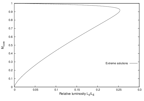
Figure 3 presents the bifurcation curve for $\alpha=0.9$. The bifurcation point with the luminosity $L_{0}=0.31130L_{E}$ on the extreme curve corresponds to a subsonic solution (see Fig. 8 for the behaviour of its speed of sound and of the infall velocity).

A transonic solution exists for $L_{0}=0.1L_{E}$, $\alpha=0.9$ on the lighter branch, but the partner lying on the more massive branch is a subsonic flow, as shown in Fig. 4.

Figure 5 shows how squares of the speed of sound $a^{2}$ and of the spatial velocity $U^{2}/k^{2}$ depend on $R$ for different gas abundances. The flow with greater gas abundance (hence with a relatively lighter compact center) possesses a sonic point that is closer to the center than in the other case. Intuitive explanation is that for greater gas density the radiation pressure is bigger and prohibits quick falloff; the infall velocity can approach the speed of sound only close to the gravity center.

Figure 6 sketches the behaviour of the speed of sound and $U^{2}/k^{2}$ for one of the subsonic solutions, with identical boundary data – but different baryonic densities – as for the flows depicted in Fig. 5.

The next figure shows characteristics of the bifurcation solution for the binding energy parameter $\alpha=0.0025$. The striking feature is that the content of gas abundance approaches $0.31$. We observed earlier that in the pure hydrodynamic accretion [4] the maximum accretion rate occurs when the gas abundance is equal to $1/3$. That is valid both in the general-relativistic [4] and newtonian [21] case. In the Shakura model [1] one can analytically prove that at the bifurcation point the luminosity is maximal and the gas abundance must be smaller that $1/3$. The inspection of Figures 1 – 3 shows that this property is satisfied also in the general-relativistic case. Here brightest flows coincide with bifurcation points. Their gas abundance is always smaller than 1/3 and decreases with the increase of $L_{0}/L_{E}$.

The last figure displays the dependence of $a^{2}$ and $U^{2}/k^{2}$ on the area radius $R$ in the case of the most luminous solutions corresponding to $\alpha=0.9$. It is clear that it is a subsonic flow.

The present analysis is fully general-relativistic, with the backreaction effects included. The picture emerging here is different from the former investigation of spherical accretion in which the space-time geometry has been fixed and therefore backreaction has been ignored [22]. The main new feature is the existence of an upper limit for the asymptotic baryonic mass density and of a massive bifurcation branch. The new striking element is the fact that the brightest configuration is unique for given redshift $\alpha$ and asymptotic speed of sound. In the case of low $\alpha$ (which is associated with low luminosity) the brightest object flow is rich in gas — about 1/3 of its mass is in the gaseous accreting matter [4].

On the other hand general-relativistic radiating systems with accreting gas behave in a qualitatively similar way to selfgravitating newtonian ones for small redshifts (i.e., for small binding energies). In both cases one observes the following feature: two arms of the bifurcation curve of transonic flows embrace, in the diagram $L_{0}-m(R_{0})$ (or the gas abundance versus asymptotic luminosity $L_{0}$), a set of subsonic solutions (see Fig. 1). For given asymptotic data ($M$ — the total mass, $L_{0}$ — asymptotic luminosity and $a^{2}_{\infty}$ — the asymptotic speed of sound) there exist two transonic solutions and an infinite number of subsonic solutions with intermediate baryonic densities. The mass of the central core in subsonic flows is comprised between two bounds of the two limiting transonicflows. The bifurcation point, where the two supersonic branches cross and the luminosity is maximal for a given (binding energy) parameter $\alpha$, is unique.

Some features of this picture change in the case of larger redshifts. This happens at some value of the parameter $\alpha$ larger than $10^{-2}$. The massive part of the bifurcation curve is replaced by a curve of subsonic solution (inspect Figs 2 and 3). Transonic flows survive only on that section of the test fluid bifurcation branch where most of the mass is comprised in the compact core and the luminosity is relatively low. One observes (for instance for $\alpha=0.5$ and $\alpha=0.9$) that as one increases the total luminosity $L_{0}$, the transonic flows completely cease to exist on the bifurcation curve and they are replaced by subsonic solutions. Nevertheless the set of all flows has a similar shape that in the case of small $\alpha$, as exemplified in Fig. 1 – 3. Subsonic solutions are not specified uniquely for given boundary data, as we point out earlier, but the length of the interval of allowed values of the asymptotic baryonic density $\rho_{0\infty}$ becomes shorter with the increase of $L_{0}$. The solution corresponding to the maximal luminosity is unique. In particular flows corresponding to highest possible luminosities (that can be close to the Eddington luminosity $L_{E}$ if $\alpha$ is close to $1$) are uniquely determined.

Finally, it is interesting that quasi-stationary solutions of the model considered in this paper can have a significant abundance of the gas. Accreting systems with maximal luminosities (in particular close to the Eddington luminosity) can possess even 33% of gas for small redshifts and still almost 10% of gas for $\alpha=0.9$. It is an open and important question whether this picture is valid for generic nonspherical flows.

This paper has been partially supported by the MNII grant 1PO3B 01229. Zdobysław Świerczyński thanks the Pedagogical University for the research grant. Krzysztof Roszkowski thanks the Foundation for Polish Science for financial support.

References

- [1] J. Karkowski, E. Malec and K. Roszkowski, Astronomy and Astrophysics, 479, 161(2008).
- [2] E. Malec and K. Roszkowski, Journal of Physics, C66, 012062(2007).
- [3] K. Roszkowski, Acta Phys. Pol. B38, 3925(2007).
- [4] J. Karkowski, E. Malec, B. Kinasiewicz, P. Mach and Z. Świerczyński, Phys. Rev. D73, 021503(R)(2006).
- [5] Thorne, K. S. and Zytkow, A. N., ApJ, 212, 832(1977).
- [6] Mazur, P. O. and Mottola, E., Proc. Nat. Acad. Sci., 101, 9545(2004)
- [7] D. Mihalas and B. W. Mihalas, Foundation of Radiation Hydrodynamics, Oxford University Press New York Oxford 1984.
- [8] M. Iriondo, E. Malec and N. O’ Murchadha, Phys. Rev. D54, 4792(1996)
- [9] M.-G. Park & G. S. Miller ApJ, 371, 708(1991).
- [10] L. Rezzolla & J. C. Miller, Class. and Quantum Grav., 11, 1815(1994).
- [11] K. S. Thorne, R. A. Flammang & A. N. Żytkow, MNRAS, 194, 475(1981).
- [12] E. Malec, Phys. Rev. D60, 104043(1999).
- [13] H. Bondi, Mon. Not. R. Astron. Soc. 112, 192(1952).
- [14] L. Schwarz, Analyse Mathematique (Paris: Hermann) 1967.
- [15] P. Padmanabhan, Theoretical Astrophysics, Vol. 1: Astrophysical Processes, Cambridge University Press, 2000.
- [16] N. I. Shakura, 1974, Astr. Zh, 51, 441(1974).
- [17] P. Mach, Acta Phys. Pol. B38, 3935(2007); B. Kinasiewicz, P. Mach and E. Malec, Int. J. of Geometric Meth. in Mod. Phys. 4, 197(2007).
- [18] B. Schutz, A First Course in General Relativity, Cambridge University Press, 1997.
- [19] J. Karkowski and E. Malec, Classical and Quantum Gravity 20, 85-92, (2003).
- [20] E. Hairer, S.P. Norsett and G. Wanner, Solving Ordinary Differential Equations I. Nonstiff Problems. 2nd Edition, Springer Series in Computational Mathematics, Springer-Verlag, 1993.
- [21] B. Kinasiewicz, PhD thesis, Jagiellonian University 2007.
- [22] F. C. Michel, Astrophys. Space Sci. 15, 153(1972); M.-G. Park and UJ. P. Ostriker,Astrophysics J. 347; 679 (1989); A. Babul et al., Astrophysics J, 347, 59 (1989); M.-G. Park, Astronomy and Astrophysics, 274, 642(1993).