Stability of the U(1) spin liquid with spinon Fermi surface in 2+1 dimensions

Fractionalized phase is a novel state of correlated many-body systems where low energy excitations carry fractional quantum numbers of microscopic degrees of freedom. In 1+1D, a spin-charge separation, which is an example of fractionalization, can naturally occur due to the low dimensionality[1]. In 2+1D, fractional quantum Hall states support excitations which have fractional electric charges[2]. Finding a fractionalized phase in time-reversal symmetric 2+1D systems is an outstanding problem in condensed matter physics[3, 4].

In fractionalized phases, there exist non-local correlations which are not captured by the conventional symmetry breaking picture[5]. Those correlations are associated with a condensation of stringy objects in space[6] or membranes in space-time[7]. It turned out that the most natural framework to describe those correlations is gauge theory, where the gauge field describes transverse fluctuations of condensed strings or membranes.

Spin liquid is a fractionalized state where an elementary excitation is spinon which carries spin $1/2$ but no charge[3]. Among a variety of possible spin liquid states[5], the state which has fermionic spinons and an emergent U(1) gauge field has been proposed for many 2+1D strongly correlated electron systems including high temperature superconductors, frustrated magnets and heavy fermion systems. Although high $T_{c}$ superconductors have the conventional superconducting ground state, the normal state shows non-Fermi liquid behaviors which are possibly due to a proximity to a spin liquid state[4, 11]. Frustrated magnets are simpler systems than the high $T_{c}$ cuprates in that there is no low energy charge mode. At the moment, there are promising candidate materials[12, 13] for which the U(1) spin liquid states with fermionic spinons have been proposed[8, 9, 10]. Related fractionalized phases have been studied in heavy fermion systems near magnetic quantum critical points[14] and frustrated bose systems[15]. In the U(1) spin liquid states, fermionic spinons have either nodal points or Fermi surfaces. The gapless spinons are strongly coupled with the U(1) gauge field at low energies and there is no well-defined quasiparticle[16, 17, 18, 19, 20, 21].

Because of underlying lattice structures, the U(1) gauge field is compact, which allows for a topological defect called instanton (or monopole). Instanton, as a localized object in space-time, describes an event where the flux of the gauge field changes by $2\pi$. Understanding dynamics of instantons is crucial because the fractionalized state is stable only if instantons are suppressed in the long distance limit. It has been known that if there is no gapless spinon, instantons always proliferate, resulting in confinement. In this case, spin liquid states are not stable and spinons are permanently confined[22]. In the presence of gapless spinons, it is possible that the gauge field is screened and instanton becomes irrelevant in the low energy limit. If this happens, fractionalized phase is stable and spinons arise as low energy excitations.

If there are a large number of gapless spinons which have the relativistic dispersion near nodal points, it has been shown that instanton is irrelevant at low energies and the fractionalized phase is stable[23]. However, it is largely unknown whether the spin liquid phase is stable in the physical cases where the number of spinon flavors is relatively small. In the presence of spinon Fermi surface, it has been speculated that the abundance of low energy spinon modes may stabilize the fractionalized phase more easily. However, dynamics of instantons in the presence of non-relativistic spinons has not been well understood. There have been several RPA studies[24, 25, 26, 27, 28, 29], but currently there exists no non-perturbative analysis on the fate of instantons in the presence of spinon Fermi surface. Particularly, a lack of the conformal symmetry makes it hard to treat the problem in a non-perturbative way which is required because instanton itself is a non-perturbative phenomenon.

In this paper, we provide a non-perturbative argument which supports the idea that the U(1) spin liquid state with spinon Fermi surface is indeed stable against proliferation of instantons for any nonzero $N$, where $N$ is the number of spinon flavors. The paper consists of the three parts. In the first part (Sec. III), we ignore fluctuations of the non-compact component of the gauge field and calculate the scaling dimension of instanton at the fixed point described by free spinons. To do this, in Sec. II, we formulate low energy modes near the Fermi surface in terms of an infinite number of 1+1D chiral fermions. Since an instanton is a localized source of $2\pi$ flux in space-time, the fermions which move in 1+1 dimensional subspaces have to enclose the half of the solid angle around the instanton and acquire phase $\pi$, when they are transported around the instanton at a sufficiently large distance. This is illustrated in Fig. 2. Therefore, an instanton operator corresponds to a twist operator of the 1+1D chiral fermions. The scaling dimension of an instanton is infinite because there are infinitely many 1+1D fermions parametrized by the direction of their velocities (or angular momentum), and each fermion contributes a finite scaling dimension to the total scaling dimension of the instanton operator. In the second part (Sec. IV), the fluctuations of the non-compact gauge field are considered together with instantons. To control the gauge fluctuations, we consider a large $N$ limit. In this case, vertex corrections are negligible and we can obtain a definite scaling transformation under which the low energy theory remains invariant. The key difference from the previous studies[19, 21] is that in the present approach all points on the Fermi surface are treated on the equal footing rather than focusing on a local patch in the momentum space. This enables us to define the scaling dimension of the instanton operator, taking into account the whole Fermi surface. With the fluctuating non-compact gauge field, fermion modes which have different Fermi velocities are no longer decoupled, and we can not simply sum the scaling dimensions of different modes as we did in the non-interacting case. However, in the low energy limit, only small angle scatterings are important because momenta of the gauge field are scaled down while the circumference of the Fermi surface is unchanged under the scale transformation. This implies that two fermion fields on different points on the Fermi surface are essentially decoupled at low energies. Therefore, there are still infinitely many independent 1+1D fermion modes which contribute to the scaling dimension of instanton at low energies. By using this property, we can argue that the scaling dimension of an instanton is infinite at the interacting fixed point too. Finally, in Sec. V, we consider the case with a small $N$ of the order of $1$ which is directly pertinent to the U(1) spin liquid state with two flavors (spin up and down) of spinons[8, 9] proposed for $\kappa-(BEDT-TTF)_{2}Cu_{2}(CN)_{3}$[12]. With a small $N$, the Fermi surface is strongly coupled with the fluctuating gauge field and vertex corrections can not be ignored. This makes it difficult to find an explicit form of a scaling transformation for the strongly interacting fixed point. However, one can see that the essential properties which make the scaling dimension of instanton infinite does not depend on the specific form of a scaling transformation. Actually, the existence of an extended Fermi surface and the fact that only small angle scatterings are important at low energies are enough to argue that the scaling dimension of instanton remains to be infinite and instantons are irrelevant at the strongly interacting fixed point for any nonzero $N$.

We start by considering $N$ flavors of fermions coupled with a compact U(1) gauge field in 2+1D,

	$\displaystyle S$	$\displaystyle=$	$\displaystyle\int d^{3}x\Bigl[\Psi_{j}^{*}(\partial_{0}-ia_{0}-\mu_{F})\Psi_{j}$		(1)
			$\displaystyle+\frac{1}{2m}\Psi_{j}^{*}(-i{\bf\nabla}-{\bf a})^{2}\Psi_{j}+\frac{1}{4g^{2}}f_{\mu\nu}f_{\mu\nu}\Bigr].$

Here $\Psi_{j}$ is the fermion field with $N$ flavors, $j=1,2,..,N$ and $a_{\mu}=(a_{0},{\bf a})$ is the U(1) gauge field with $\mu=0,1,2$. $\mu_{F}$ is the chemical potential and $g$, the gauge coupling. $f_{\mu\nu}$ is the field strength tensor. Summation over the repeated flavor index $j$ is implied. In the energy-momentum space, the action becomes

	$\displaystyle S=\int d^{3}p~~\Bigl[(ip_{0}+\epsilon_{\bf p})\Psi_{j}^{*}(p)\Psi_{j}(p)+\frac{1}{2g^{2}}\left(p^{2}\delta_{\mu\nu}-p_{\mu}p_{\nu}\right)a_{\mu}^{*}(p)a_{\nu}(p)\Bigr]$
	$\displaystyle+\int\frac{d^{3}pd^{3}l}{(2\pi)^{3/2}}~~\left(-ia_{0}(l)-\frac{{\bf p}\cdot{\bf a}(l)}{m}\right)\Psi_{j}^{*}(p+\frac{l}{2})\Psi_{j}(p-\frac{l}{2})$
	$\displaystyle+\int\frac{d^{3}p_{1}d^{3}p_{2}d^{3}l}{(2\pi)^{3}}~~\frac{1}{2m}{\bf a}^{*}(p_{2}-l)\cdot{\bf a}(p_{2})\Psi_{j}^{*}(p_{1}+l)\Psi_{j}(p_{1}).$

Here $p$, $l$ denote energy-momentum vectors and $\epsilon_{\bf p}=\frac{|{\bf P}|^{2}}{2m}-\mu_{F}$. Integrating out high energy fermion modes outside a momentum shell with a width $\Lambda$ near the Fermi surface, we obtain the low energy effective action $S=S_{0}+S_{1}$, where

	$\displaystyle S_{0}=\int d\omega dkd\theta~~\left(i\omega+k\right)\psi_{j}^{*}(\omega,k,\theta)\psi_{j}(\omega,k,\theta)$
	$\displaystyle+\int d^{3}p\left(\frac{1}{2g^{2}}\left[p^{2}\delta_{\mu\nu}-p_{\mu}p_{\nu}\right]a_{\mu}^{*}(p)a_{\nu}(p)+K{\bf a}^{*}(p)\cdot{\bf a}(p)\right),$
	$\displaystyle S_{1}=-\frac{i}{(2\pi)^{3/2}}\int d\omega dkd\theta d\nu dq_{l}dq_{t}~\Bigl(a_{0}(\nu,q_{l},q_{t};\theta)-ia_{\theta}(\nu,q_{l},q_{t};\theta)\Bigr)\times$
	$\displaystyle\psi_{j}^{*}(\omega+\frac{\nu}{2},k+\frac{q_{l}}{2},\theta+\frac{q_{t}}{2k_{F}})\psi_{j}(\omega-\frac{\nu}{2},k-\frac{q_{l}}{2},\theta-\frac{q_{t}}{2k_{F}}).$
			(3)

Here, the Fermi velocity has been set to $1$. Fermion momentum is represented in the polar coordinate[30] where $k\equiv|\textbf{k}|-k_{F}$ is the deviation of momentum from the Fermi surface in the radial direction and $\theta$ is the angular coordinate as is shown in Fig. 1 (a). We use the approximation, $\int d\textbf{k}=\int d|\textbf{k}||\textbf{k}|\int d\theta\approx k_{F}\int dk\int d\theta$ and redefine the fermion field as $\psi_{j}(\omega,k,\theta)\equiv k_{F}^{1/2}\Psi_{j}\left(\omega,k_{1}=(k_{F}+k)\cos\theta,k_{2}=(k_{F}+k)\sin\theta\right)$. $K\sim Nk_{F}$ is the diamagnetic term. $a_{\theta}=\hat{k}_{\theta}\cdot{\bf a}$ is the spatial gauge field parallel to the fermion momentum along $\hat{k}_{\theta}=(\cos\theta,\sin\theta)$. $q_{l}=\hat{k}_{\theta}\cdot{\bf q}$ and $q_{t}=(\hat{k}_{\theta}\times{\bf q})_{z}$ are the momentum components of the gauge field which are parallel and perpendicular to $\hat{k}_{\theta}$ respectively. Note that $a_{0}(\nu,q_{l},q_{t};\theta)$ and $a_{\theta}(\nu,q_{l},q_{t};\theta)$ in the second line of Eq. (3) implicitly depend on $\theta$ because $q_{l}$ and $q_{t}$ are measured with reference to $\hat{k}_{\theta}$ as is shown in Fig. 1 (b). $\Lambda$ is the momentum cut-off of the fermions near the Fermi surface and $\tilde{\Lambda}$ is the cut-off of the gauge field. For $\Lambda<<k_{F}$, we can ignore the quadratic term $k^{2}/2m$ which is irrelevant at low energies.

The gauge field can be decomposed into the singular part which includes instanton configurations and the non-singular part which describes fluctuations of the non-compact component. First, we ignore the non-compact gauge field and examine the effect of instantons on the free fermions. For this, we consider a background gauge field $a_{\mu}^{s}$ generated by an instanton located at $\tau=0$ and $\textbf{x}=0$ in space and time. For the singular part of the gauge field, we use the temporal gauge where $a_{0}^{s}=0$.

If the Fermi surface has the rotational symmetry, the field strength for single instanton centered at the origin has the rotational symmetry too. This enables us to choose $a_{\theta}^{s}(\nu,q_{l},q_{t};\theta)$ to be independent of $\theta$. Because of the rotational symmetry, it is convenient to introduce 1+1D chiral Fermi fields which have good angular momentum quantum number,

$$\psi_{jn}(\tau,x)=\frac{1}{(2\pi)^{3/2}}\int d\omega dkd\theta~e^{i(\omega\tau+kx+n\theta)}\psi_{j}(\omega,k,\theta).$$

(4)

In the 1+1D real space, the action for the chiral fermions becomes

	$\displaystyle S$	$\displaystyle=$	$\displaystyle\sum_{n}\int d\tau dx~\psi_{jn}^{*}(\tau,x)\Bigl[\partial_{\tau}$		(5)
			$\displaystyle~~~-i(\partial_{x}-ia_{\theta}^{s}(\tau,x,x_{t}=n/k_{F}))\Bigr]\psi_{jn}(\tau,x),$

where the 1+1D gauge field ‘felt’ by the chiral fermions is given by

	$\displaystyle a^{s}_{\theta}(\tau,x,x_{t})$	$\displaystyle=$	$\displaystyle\frac{1}{(2\pi)^{3/2}}\int_{-\infty}^{\infty}d\omega\int_{-\Lambda/2}^{\Lambda/2}dq_{l}\int_{-\tilde{\Lambda}}^{\tilde{\Lambda}}dq_{t}$		(6)
			$\displaystyle e^{i(\omega\tau+q_{l}x+q_{t}x_{t})}a_{\theta}^{s}(\omega,q_{l},q_{t};\theta).$

Here $x$ and $x_{t}$ represent the displacements from the instanton in the directions parallel and perpendicular to $\hat{k}_{\theta}$ for some $\theta$ respectively. Because of the rotational symmetry, $a_{\theta}(\tau,x,x_{t})$ is independent of $\theta$ and the choice of $\theta$ does not matter. The action in Eq. (5) describes an infinite set of 1+1D chiral fermions coupled to the background gauge field, $a_{\theta}^{s}(\tau,x,x_{t}=n/k_{F})$. The chiral fermion with angular momentum $n$ ‘sees’ the 2+1D gauge field projected onto a plane which is perpendicular to the $x_{1}-x_{2}$ plane and shifted by $n/k_{F}$ away from the origin as is shown in Fig. 2 (a). The range of the momentum integration in Eq. (6) is restricted to be within the strip with the width $\Lambda$ as is shown in Fig. 1 (b) and $a^{s}_{\theta}(\tau,x,x_{t})$ represents slowly varying configurations of the gauge field in space and time. Nevertheless, the components with large momenta become unimportant in the long distance limit, and $a^{s}_{\theta}(\tau,x,x_{t})$ accurately describes the true configuration of instanton far away from the center. For an instanton whose field strength is isotropic in space and time, the gauge field is given by

	$\displaystyle a_{0}$	$\displaystyle=$	$\displaystyle 0,$
	$\displaystyle a_{1}$	$\displaystyle=$	$\displaystyle\frac{x_{2}}{2r(r-\tau)},$
	$\displaystyle a_{2}$	$\displaystyle=$	$\displaystyle-\frac{x_{1}}{2r(r-\tau)},$		(7)

with $r=\sqrt{\tau^{2}+x_{1}^{2}+x_{2}^{2}}$. In this gauge, there is a Dirac string stretched along the positive $\tau$ axis. The presence of the Dirac string is not important because the infinitely thin tube of $2\pi$ flux can always be placed inside a halo of an underlying lattice and the unit flux can be gauged away. The gauge field in Eq. (7) represents an instanton with the Lorentz symmetry. In the presence of the non-relativistic fermions, the space-time isotropy is lost and the field strength will be redistributed. With the broken Lorentz symmetry, the spatial rotational symmetry in the $x_{1}-x_{2}$ space may or may not be broken. In the following, we will first consider the case with the spatial rotational symmetry and then consider general cases without the symmetry.

As an 1+1D fermion is transported within a plane at distance $L$ from its origin as in Fig. 2 (a), it encloses the solid angle, $\Omega_{n}(L)=2\pi\left(1-\frac{n}{\sqrt{(Lk_{F})^{2}+n^{2}}}\right)$ in the unit sphere around the instanton as is shown in Fig. 2 (b). Since an instanton is the source of flux $2\pi$, the fermion acquires a non-trivial phase $\Phi_{n}(L)$. Without loss of generality, we can defined the phase angle within the interval $(-\pi,\pi]$. For the Lorentz symmetric instanton configuration in Eq. (7), the phase angle is the half of the solid angle and becomes

$$\Phi_{n}(L)=sgn(n)\pi\left(1-\frac{|n|}{\sqrt{(Lk_{F})^{2}+n^{2}}}\right).$$

(8)

For non-isotropic configurations, $\Phi_{n}(L)$ will be different from Eq. (8). However, the explicit form of $\Phi_{n}(L)$ is not important for the following discussions. What is important is the fact that $|\Phi_{n}(L)|\rightarrow\pi$ for any finite $n$ as $L\rightarrow\infty$ in the presence of the spatial rotational symmetry. This is because trajectories of fermions projected onto the unit sphere around the instanton will eventually follow a big circle for any angular momentum $n$ in the large $L$ limit, and the flux enclosed by any half sphere that cuts through the north and south poles is always $\pi$ due to the spatial rotational symmetry. Therefore, in the long distance limit, an instanton twists boundary conditions of all fermions from the periodic condition to the anti-periodic one. Roughly speaking, at a length scale $L$, an instanton twists boundary conditions of the fermions which have angular momenta $|n|<k_{F}L$ by $\pi$.

Having understood that an instanton operator corresponds to a twist operator, we can determine the scaling dimension of instanton. To do this, we represent the 1+1D space in terms of a complex variable, $z=\tau-ix$ and rescale the fermion fields to write the action in the standard form,

$\displaystyle S_{free}=\frac{1}{2\pi}\sum_{j=1}^{N}\sum_{n=-\infty}^{\infty}\int dzd{\bar{z}}~~\psi_{jn}^{*}{\bar{\partial}}\psi_{jn},$

(9)

where $\bar{\partial}=\frac{\partial}{\partial\bar{z}}$. This free theory is invariant under the scale transformation,

	$\displaystyle z$	$\displaystyle=$	$\displaystyle bz^{{}^{\prime}},$
	$\displaystyle\bar{z}$	$\displaystyle=$	$\displaystyle b\bar{z}^{{}^{\prime}},$
	$\displaystyle\psi_{jn}(b\tau^{{}^{\prime}},bx^{{}^{\prime}})$	$\displaystyle=$	$\displaystyle b^{-1/2}\psi_{jn}^{{}^{\prime}}(\tau^{{}^{\prime}},x^{{}^{\prime}})$		(10)

with $b>1$. With instantons, the free theory is perturbed as

$\displaystyle S=S_{free}+y\int dzd\bar{z}~~\sigma,$

(11)

where $\sigma$ is the creation operator of an instanton or an anti-instanton and $y$ is the fugacity. Since an instanton twists the boundary conditions of all fermions in the low energy limit, the instanton operator can be written as

$\displaystyle\displaystyle\sigma=\Pi_{j,n}\sigma_{jn}(\pi),$

(12)

where $\sigma_{jn}(\pi)$ is the operator which twists the boundary condition of $\psi_{jn}$ by $\pi$. However, the scaling dimension of $\sigma$ is not well-defined because the operator ends up twisting the infinite number of fermions by the finite angle, $\pi$. Actually, not all fermions are twisted by the same angle at a finite length scale $L$[31]. Therefore we introduce a regularized instanton operator,

$\displaystyle\displaystyle\sigma_{L}=\Pi_{j,n}\sigma_{jn}(\Phi_{n}(L)),$

(13)

where $\sigma_{jn}(\Phi_{n}(L))$ is an operator which twists the boundary condition of $\psi_{jn}$ by the angle $\Phi_{n}(L)$. Physically, $\sigma_{L}$ creates the flux configuration near an instanton at a length scale $L$. Although $\sigma_{L}$ is not a true instanton operator, we can learn about the property of the true instanton by taking $L\rightarrow\infty$ limit of $\sigma_{L}$. The point of introducing the regularized operator is that $\sigma_{L}$ is a well defined local operator which has a finite scaling dimension, as will be shown below.

Since the scaling dimension corresponds to the eigenvalue of the scale transformation generated by the Noether current $j_{\nu}=x^{\mu}T_{\mu\nu}$, the scaling dimension $d_{L}$ of the regularized instanton operator can be obtained from

$\displaystyle d_{L}\sigma_{L}(0)=\oint\frac{dz}{2\pi i}~~zT(z)\sigma_{L}(0),$

(14)

where $T(z)$ is the holomorphic energy momentum tensor. In the state-operator correspondence, we can view the scaling dimension as the ‘energy’ of the quantum state defined on the circle around the origin associated with the ‘time’ evolution in the radial direction. What the insertion of the $\sigma_{L}$ operator does is to twist the boundary condition of $\psi_{jn}$ by $\Phi_{n}(L)$. Then we can rewrite Eq. (14) as

$\displaystyle d_{L}=\left<\oint\frac{dz}{2\pi i}~~zT(z)\right>_{twisted~b.c.},$

(15)

where we impose the twisted boundary condition for the fermion fields around the origin. Each fermion $\psi_{jn}$ contribute a scaling dimension $d(\Phi_{n}(L))=\frac{\Phi_{n}(L)^{2}}{8\pi^{2}}$ (see appendix A for derivation) and the total scaling dimension for the regularized instanton operator becomes

$\displaystyle d_{L}$

$\displaystyle=$

$\displaystyle\sum_{j=1}^{N}\sum_{n=-\infty}^{\infty}\frac{\Phi_{n}(L)^{2}}{8\pi^{2}}.$

(16)

Since $\Phi_{n}(L)$ approaches $\pi$ as $L$ increases, $d_{L}$ diverges in the large $L$ limit. For the isotropic instanton configuration, we have

$\displaystyle d_{L}^{isotropic}$

$\displaystyle=$

$\displaystyle\sum_{j=1}^{N}\sum_{n=-\infty}^{\infty}\frac{1}{8}\left(1-\frac{|n|}{\sqrt{(Lk_{F})^{2}+n^{2}}}\right)^{2},$

(17)

and it is easy to check that it diverges linearly with $L$. The renormalization group equation for the fugacity becomes

$\displaystyle\frac{dy_{L}}{d\ln b}=\left(2-d_{L}\right)y_{L}+O(y_{L}^{2}),$

(18)

where $y_{L}$ is the fugacity of the regularized instanton operator. The present approach does not allow us to calculate the higher order terms in $y$. However, from the linear term alone, we can readily see that for any $N>0$ the regularized instanton operator for a sufficiently large $L$ (hence the true instanton operator defined as $\sigma=\lim_{L\rightarrow\infty}\sigma_{L}$) is strongly irrelevant at the fixed point with $y=0$. Namely, a small nonzero $y$ will flow to the fixed point with $y=0$. Although the scaling dimension of the true instanton operator defined as $d=\lim_{L\rightarrow\infty}d_{L}$ is ill-defined (infinite) for any $N>0$, the regularized scaling dimension diverges more rapidly with increasing $L$ when $N$ is larger. This is consistent with the physical intuition that the presence of more fermions results in a larger scaling dimension of instanton via screening.

Until now, we have considered the case with the spatial rotational symmetry. If the symmetry is broken by an underlying lattice, the field configuration of an instanton is no longer symmetric under the spatial rotation. Here we will see that the conclusion reached for the rotationally symmetric Fermi surface holds in general cases too as far as the general Fermi surface can be obtained from the symmetric one through a smooth deformation. Performing the Fourier transformations for the frequency and the radial momentum, we rewrite $S_{1}$ in Eq. (3) as

	$\displaystyle S_{1}=-\frac{1}{(2\pi)^{1/2}}\int d\tau dxd\theta d\theta^{{}^{\prime}}$
	$\displaystyle a_{\theta}(\tau,x,k_{F}(\theta-\theta^{{}^{\prime}});(\theta+\theta^{{}^{\prime}})/2)\psi_{j}^{*}(\tau,x,\theta)\psi_{j}(\tau,x,\theta^{{}^{\prime}}).$

For a general Fermi surface, $a_{\theta}$ has a non-trivial angular dependence on $(\theta+\theta^{{}^{\prime}})/2$. To diagonalize the action, we have to use a different basis than the angular momentum basis. We consider the basis transformation,

$$\psi_{jn}(\tau,x)=\frac{1}{(2\pi)^{1/2}}\int d\theta~f_{n}^{*}(\tau,x,\theta)\psi_{j}(\tau,x,\theta),$$

(20)

where $f_{n}(\tau,x,\theta)$ satisfies the eigenvalue equation,

	$\displaystyle\frac{1}{(2\pi)^{1/2}}\int d\theta^{{}^{\prime}}a_{\theta}(\tau,x,k_{F}(\theta-\theta^{{}^{\prime}});(\theta+\theta^{{}^{\prime}})/2)f_{n}(\tau,x,\theta^{{}^{\prime}})$
	$\displaystyle=a_{n}(\tau,x)f_{n}(\tau,x,\theta)$		(21)

and the normalization condition

$\displaystyle\frac{1}{2\pi}\int d\theta~f_{m}^{*}(\tau,x,\theta)f_{n}(\tau,x,\theta)=\delta_{m,n}.$

(22)

One can always find such a basis because the kernel $a_{\theta}$ satisfies the Hermitian condition, $a_{\theta}(\tau,x,k_{F}(\theta-\theta^{{}^{\prime}});(\theta+\theta^{{}^{\prime}})/2)=a_{\theta}^{*}(\tau,x,-k_{F}(\theta-\theta^{{}^{\prime}});(\theta+\theta^{{}^{\prime}})/2)$ at each $\tau$ and $x$. In the new basis, the action for the 1+1D chiral fermions becomes diagonal,

	$\displaystyle S$	$\displaystyle=$	$\displaystyle\sum_{n}\int d\tau dx~\psi_{jn}^{*}(\tau,x)\Bigl[\partial_{\tau}$		(23)
			$\displaystyle-i(\partial_{x}-ia_{n}(\tau,x))\Bigr]\psi_{jn}(\tau,x).$

The phase acquired by the $n$-th fermion when the fermion is transported around the instanton is

$\displaystyle\Phi_{n}=\oint dxa_{n},$

(24)

and the total scaling dimension becomes

$\displaystyle d=N\sum_{n}\frac{\Phi_{n}^{2}}{8\pi^{2}},$

(25)

where $-\pi<\Phi_{n}\leq\pi$. For the rotationally symmetric Fermi surface, the index $n$ represents the angular momentum as before and $\Phi_{n}=\pi$ for all $n$ in the low energy limit. As the Fermi surface (hence the field configuration of an instanton) is distorted, the distribution of $\Phi_{n}$ gets broadened around $\pm\pi$ and $d$ will decrease. However, $d$ can not change abruptly as the Fermi surface is smoothly deformed and $d$ will remain infinite in the thermodynamic limit unless there is a phase transition associated with the topology of the Fermi surface. Therefore, the scaling dimension of an instanton is infinite for a general Fermi surface as far as the Fermi surface is smoothly connected to the rotationally symmetric Fermi surface.

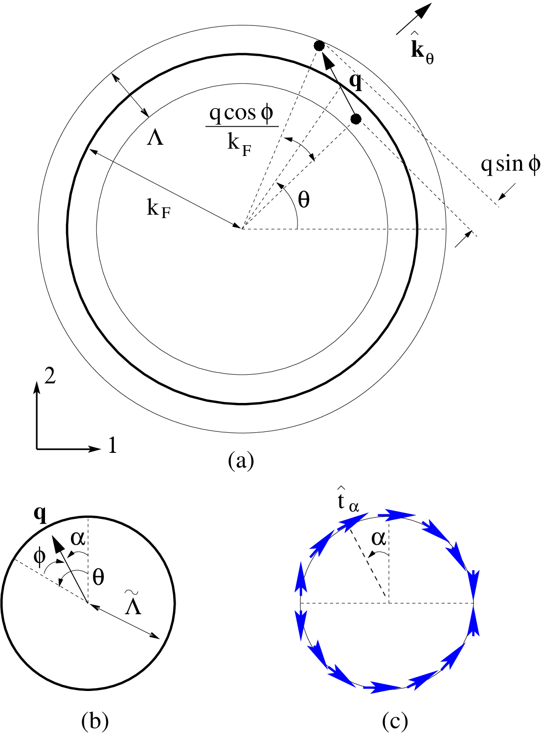
Now we consider the whole theory by taking into account fluctuations of the non-compact gauge field. For the non-compact gauge field, we will use the Coulomb gauge where ${\bf\nabla}\cdot{\bf a}=0$[32] and drop the temporal gauge field which is screened out at long distances. In the following, we will focus on the rotationally symmetric case. With the fluctuating non-compact gauge field, the interaction term can be written as

	$\displaystyle S_{1}=\frac{-1}{(2\pi)^{3/2}}\int_{-\infty}^{\infty}d\omega\int_{-\frac{\Lambda}{2}}^{\frac{\Lambda}{2}}dk\int_{-\pi}^{\pi}d\theta\int_{-\infty}^{\infty}d\nu\int_{0}^{\tilde{\Lambda}}dqq\int_{-\pi}^{\pi}d\phi$
	$\displaystyle~~~\Theta\left(\Lambda/2-\left|k+q\sin\phi/2\right|\right)\Theta\left(\Lambda/2-\left|k-q\sin\phi/2\right|\right)\hat{k}_{\theta}\cdot\hat{t}_{\theta-\phi}a(\nu,q,\theta-\phi)\times$
	$\displaystyle\psi_{j}^{*}\left(\omega+\nu/2,k+q\sin\phi/2,\theta+q\cos\phi/2k_{F}\right)\psi_{j}\left(\omega-\nu/2,k-q\sin\phi/2,\theta-q\cos\phi/2k_{F}\right),$
			(26)

where $a$ is the transverse gauge field. The momentum of the gauge field is also written in the polar coordinate as $a(\nu,q,\alpha)=a(\nu,q_{1}=-q\sin\alpha,q_{2}=q\cos\alpha)$. $\hat{t}_{\alpha}$ is the polarization vector of the gauge field with an angle $\alpha$, where the angle is defined in such a way that $\hat{t}_{\alpha}$ becomes parallel to $\hat{k}_{\theta}$ when $\alpha=\theta$ as is depicted in Fig. 3. We choose the polarization vector as $\hat{t}_{\alpha}=(\cos\alpha,\sin\alpha)$ for $-\pi/2\leq\alpha<\pi/2$ and $\hat{t}_{\alpha}=(\cos(\alpha+\pi),\sin(\alpha+\pi))$ for $\alpha\geq\pi/2$ or $\alpha<-\pi/2$ as is shown in 3 (c). In this definition, there are discontinuities in $\hat{t}_{\alpha}$ at $\alpha=\pm\pi/2$. However, this definition is convenient to make the reality of the gauge field explicit in the momentum space as $a(-\nu,q,\alpha+\pi)=a^{*}(\nu,q,\alpha)$. $\Theta(x)$ is the step function which ensures that the momenta of fermions lie within the shell of the width $\Lambda$ near the Fermi surface.

At low energies we have $\tilde{\Lambda}\sim\sqrt{k_{F}\Lambda}$ because the Fermi surface is locally parabolic. Since $k_{F}>>\tilde{\Lambda}>>\Lambda$, typical momenta of the gauge field are perpendicular to fermion momentum and much larger than $\Lambda$. Therefore the support of the $\phi$ integration in Eq. (26) is sharply centered at $\phi=0$ and $\phi=\pi$ with the width of the order of $\Lambda/\tilde{\Lambda}<<1$. This allows us to use $\sin\phi\approx\pm\phi$ and $\cos\phi\approx\pm 1$ in the low energy limit. Because both of the fermions with angles $\theta$ and $\theta+\pi$ are coupled with both of the gauge fields with angle $\theta$ and $\theta+\pi$, it is convenient to define two separate fields for the opposite-moving fermions and restrict the integrations of $\theta$ to run from $-\pi/2$ to $\pi/2$. At the same time, we allow $q$ to run from $-\tilde{\Lambda}$ to $\tilde{\Lambda}$ and restrict the $\phi$ integration to $-\Lambda/|q|<\phi<\Lambda/|q|$ to implement the theta functions in Eq. (26). Then the action can be written as $S=S_{0}+S_{1}$, where

	$\displaystyle S_{0}=\sum_{s=\pm 1}\int_{-\infty}^{\infty}d\omega\int_{-\Lambda/2}^{\Lambda/2}dk\int_{-\pi/2}^{\pi/2}d\theta~~\left(i\omega+sk\right)\psi_{js}^{*}\left(\omega,k,\theta\right)\psi_{js}\left(\omega,k,\theta\right)$
	$\displaystyle+\int_{-\infty}^{\infty}d\nu\int_{-\tilde{\Lambda}}^{\tilde{\Lambda}}dq|q|\int_{-\pi/2}^{\pi/2}d\alpha~~\left(\frac{1}{2g^{2}}(\nu^{2}+q^{2})+K\right)a(\nu,q,\alpha)a(-\nu,-q,\alpha),$		(27)
	$\displaystyle S_{1}=-\sum_{s=\pm 1}\frac{1}{(2\pi)^{3/2}}\int_{-\infty}^{\infty}d\omega\int_{-\Lambda/2}^{\Lambda/2}dk\int_{-\pi/2}^{\pi/2}d\theta\int_{-\infty}^{\infty}d\nu\int_{-\tilde{\Lambda}}^{\tilde{\Lambda}}dq|q|\int_{-\Lambda/|q|}^{\Lambda/|q|}d\phi$
	$\displaystyle sa(\nu,q,\theta-\phi)\psi_{js}^{*}\left(\omega+\nu/2,k+q\phi/2,\theta+sq/2k_{F}\right)\psi_{js}\left(\omega-\nu/2,k-q\phi/2,\theta-sq/2k_{F}\right),$
			(28)

where $s=1,-1$ labels fermion fields on the two sides of the Fermi surface at each angle $-\pi/2\leq\theta<\pi/2$, defined as

	$\displaystyle\psi_{j+}(\omega,k,\theta)$	$\displaystyle=$	$\displaystyle\psi_{j}(\omega,k,\theta)$
	$\displaystyle\psi_{j-}(\omega,k,\theta)$	$\displaystyle=$	$\displaystyle\psi_{j}(\omega,-k,-sgn(\theta)\pi+\theta),$		(29)

and a negative $q$ of the gauge field represents the opposite momentum as

$\displaystyle a(\nu,-|q|,\alpha)=a(\nu,|q|,\alpha+\pi)$

(30)

with $-\pi/2\leq\alpha<\pi/2$. $\psi_{j+}$ and $\psi_{j-}$ have the opposite velocities and they form a two-component 1+1D Dirac fermion.

The present approach is conceptually analogous to the bosonized descriptions of Fermi surface[33, 34, 35, 36], where chiral bosons describe low energy particle-hole excitations near Fermi surface. However, there is an important difference. In the previous bosonized description of the Fermi surface coupled with the U(1) gauge field[36], the Fermi surface is taken to be locally flat within each momentum patch, and the local curvature is not taken into account. The present formalism captures the local curvature effect of the Fermi surface, which is important to reproduce correct low energy behaviors[21]. The key is to consider all points on the Fermi surface on the equal footing, not treating the Fermi surface as a sum of locally flat Fermi segments. The way the curvature effect is implemented in Eq. (28) is explained in Fig. 4.

Here we assume that $N>>1$ in which case the fluctuations of the gauge field are controlled. In the leading order of the $1/N$ expansion, vertex corrections can be ignored[19]. The fluctuating gauge field and the gapless fermions lead to singular self energies and the single particle quantum effective action of the fermions and the transverse gauge field becomes (see appendix B)

	$\displaystyle\Gamma_{0}$	$\displaystyle=$	$\displaystyle\sum_{s=\pm 1}\int d\omega dkd\theta\left[ic~\mbox{sgn}(\omega)|\omega|^{2/3}+sk\right]$
			$\displaystyle~~~~~~~\psi_{js}^{*}(\omega,k,\theta)\psi_{js}(\omega,k,\theta)$
			$\displaystyle+\int d\nu dq|q|d\alpha\left[\gamma\frac{|\nu|}{|q|}+\chi q^{2}\right]a^{*}(\nu,q,\alpha)a(\nu,q,\alpha),$

where $c$, $\gamma$ and $\chi$ are constants. Because of the singular quantum corrections, the scaling transformation in Eq. (10) is no longer a symmetry. Instead, we have to rescale energy and momentum as

	$\displaystyle\omega$	$\displaystyle=$	$\displaystyle b^{-1}\omega^{{}^{\prime}},$
	$\displaystyle\nu$	$\displaystyle=$	$\displaystyle b^{-1}\nu^{{}^{\prime}},$
	$\displaystyle\Lambda$	$\displaystyle=$	$\displaystyle b^{-2/3}\Lambda^{{}^{\prime}},$
	$\displaystyle\tilde{\Lambda}$	$\displaystyle=$	$\displaystyle b^{-1/3}\tilde{\Lambda}^{{}^{\prime}},$
	$\displaystyle k$	$\displaystyle=$	$\displaystyle b^{-2/3}k^{{}^{\prime}},$
	$\displaystyle q$	$\displaystyle=$	$\displaystyle b^{-1/3}q^{{}^{\prime}}.$		(32)

Note that the momentum of the fermion in the radial direction and the momentum of the gauge field should scale differently. If we apply this new scale transformation to $S_{1}$ in Eq. (28), we readily notice that the action can not be made invariant unless the angular variables $\theta$ and $\phi$ are rescaled as well. This is because momenta of the fermions and the gauge field mix with the angular variables through $k+q\phi$ and $\theta+sq/k_{F}$. To make the action invariant, we should assign the scaling dimension $1/3$ to the angular variables. This is an anomalous scaling dimension of the angular variables which arises solely from quantum effects. The whole action is invariant if we rescale

	$\displaystyle\theta$	$\displaystyle=$	$\displaystyle b^{-1/3}\theta^{{}^{\prime}},$
	$\displaystyle\phi$	$\displaystyle=$	$\displaystyle b^{-1/3}\phi^{{}^{\prime}},$
	$\displaystyle\psi_{a}(b^{-1}\omega^{{}^{\prime}},b^{-2/3}k^{{}^{\prime}},b^{-1/3}\theta^{{}^{\prime}})$	$\displaystyle=$	$\displaystyle b^{4/3}\psi_{a}^{{}^{\prime}}(\omega^{{}^{\prime}},k^{{}^{\prime}},\theta^{{}^{\prime}}),$
	$\displaystyle a(b^{-1}\nu^{{}^{\prime}},b^{-2/3}q^{{}^{\prime}},b^{-1/3}\phi^{{}^{\prime}})$	$\displaystyle=$	$\displaystyle b^{4/3}a^{{}^{\prime}}(\nu^{{}^{\prime}},q^{{}^{\prime}},\phi^{{}^{\prime}})$		(33)

along with Eq. (32). As we go to lower energy ($b>1$), the range of the $\theta$ integration increases from $(-\pi/2,\pi/2)$ to $(-b\pi/2,b\pi/2)$. In the low energy limit where $b\rightarrow\infty$, $\theta$ becomes a non-compact variable which runs from $-\infty$ to $\infty$. The physical reason behind this ‘decompactification’ of the angular variable can be understood in the following way. In the low energy limit, the gauge field becomes more and more ineffective in scattering fermions from one momentum to another momentum along tangential directions to the Fermi surface. This is because the momentum of the gauge field is scaled down under the scale transformation, while the circumference of the Fermi surface is unchanged. This effectively makes two momentum points on the Fermi surface more decoupled from each other at lower energies. In other words, the ‘metric’ of the Fermi surface along the tangential directions diverges in the low energy limit compared to the ‘metric’ along the perpendicular directions.

Introducing 1+1D fields in real space,

	$\displaystyle\psi_{js}(\tau,x,\theta)$	$\displaystyle=$	$\displaystyle\frac{1}{2\pi}\int_{-\infty}^{\infty}d\omega\int_{-\Lambda/2}^{\Lambda/2}dk~~e^{i(\omega\tau+kx)}\psi_{js}(\omega,k,\theta),$		(34)
	$\displaystyle a_{q}(\tau,x,\theta)$	$\displaystyle=$	$\displaystyle\frac{1}{2\pi}\int_{-\infty}^{\infty}d\omega\int_{-\Lambda/|q|}^{\Lambda/|q|}d\phi|q|~~e^{i(\omega\tau+xq\phi)}a(\omega,q,\theta-\phi),$		(35)

we can write down the low energy effective action in the 1+1D real space as

	$\displaystyle S=\sum_{s=\pm 1}\int d\tau dxd\theta~~\psi_{js}^{*}\left(\tau,x,\theta\right)[\partial_{\tau}-is\partial_{x}]\psi_{js}\left(\tau,x,\theta\right).$
	$\displaystyle+\frac{1}{2\Lambda}\int d\tau dxd\theta dq~~|q|a_{q}^{*}(\tau,x,\theta)\left(\frac{1}{2g^{2}}(-\partial_{\tau}^{2}+q^{2})+K\right)a_{q}(\tau,x,\theta)$
	$\displaystyle-\frac{1}{(2\pi)^{1/2}}\sum_{s=\pm 1}\int d\tau dxd\theta dq~~sa_{q}(\tau,x,\theta)\psi_{js}^{*}\left(\tau,x,\theta+sq/2k_{F}\right)\psi_{js}\left(\tau,x,\theta-sq/2k_{F}\right).$		(36)

It should be emphasized that in this action $\theta$ is a non-compact variable which runs from $-\infty$ to $\infty$. In Eq. (35), $a_{q}(\tau,x,\theta)$ depends on four variables while $a(\omega,q,\theta-\phi)$ depends only on three independent variables. The variable $x$ has been created by the Fourier transformation of $a(\omega,q,\alpha)$ with respect to $\alpha$ which is centered at $\theta$. Conceptually, this is similar to creating a wave-packet which is localized in both real space and momentum space by linearly superposing wavefunctions whose momenta are centered at a particular momentum. The factor $1/2\Lambda$ in the second line of Eq. (36) is to cancel the double counting of momentum points. Note that $a_{q}(\tau,x,\theta_{1})$ and $a_{q}(\tau,x,\theta_{2})$ are not completely independent for different $\theta_{1}$ and $\theta_{2}$. Both $a_{q}(\tau,x,\theta_{1})$ and $a_{q}(\tau,x,\theta_{2})$ include contributions from a common region in the momentum space as is shown in Fig. 5. However, the overlap is not important in determing the scaling dimension of instanton as will be shown in the following. The area of the common region for $a_{q}(\tau,x,\theta_{1})$ and $a_{q}(\tau,x,\theta_{2})$ (the dark parallelogram in Fig. 5) is $(\Lambda^{2}/\Delta\theta)$ for a small $\Delta\theta=\theta_{2}-\theta_{1}$. The ratio of this area to the area included in $a_{q}(\tau,x,\theta)$ (the long strip in Fig. 5) is $\gamma=(\Lambda^{2}/\Delta\theta)/(\Lambda\tilde{\Lambda})$. As the momentum cut-off decreases as $\Lambda\rightarrow\Lambda b^{-2/3}$, $\tilde{\Lambda}\rightarrow\tilde{\Lambda}b^{-1/3}$, the ratio decreases as $\gamma\rightarrow b^{-1/3}(\Lambda/\tilde{\Lambda}\Delta\theta)$. The ratio becomes zero in the low energy limit for any nonzero $\Delta\theta$, which implies that the two fields which have a finite angle difference (before scaling) are independent in the low energy limit. In the rescaled angular variable $\theta^{{}^{\prime}}=b^{1/3}\theta$, a fixed $\Delta\theta^{{}^{\prime}}$ corresponds to a successively reduced $\Delta\theta=b^{-1/3}\Delta\theta^{{}^{\prime}}$ as a low energy limit is taken. Since $\gamma$ goes as $b^{0}$ for a fixed $\Delta\theta^{{}^{\prime}}$ in the rescaled variable, two fields which have a fixed angle different $\Delta\theta^{{}^{\prime}}$ have a finite ratio $\gamma$ in the low energy limit. On the other hand, two fields whose angle difference increases faster than $\Delta\theta^{{}^{\prime}}=b^{0}$ in the rescaled variable have vanishing overlap in the low energy limit. Since the interval of $\theta^{{}^{\prime}}$ increases as $b^{1/3}\pi$, there are infinitely many independent fields $a_{q}(\tau,x,\theta)$ which are separated in the angular direction and have only local interactions. We call this property an ‘asymptotic locality’. This will play a crucial role in determining the scaling dimension of instanton as will be discussed later.

Now we can determine the scaling dimension of the instanton operator. At a scale set by $\tau$ and $x$, fermion modes whose angular momenta are less than $n_{max}\sim k_{F}\mbox{min}(x,\tau)=k_{F}x$ are twisted (at sufficiently large distances, we always have $\tau>x$ because space has the smaller absolute scaling dimension). In other words, fermion fields that are twisted at scale $x$ have ‘wavelengths’ larger than $\delta\theta\sim 1/n_{max}\sim(k_{F}x)^{-1}$ in the space of $\theta$. Since $x$ and $\theta$ scale as $x=b^{2/3}x^{{}^{\prime}}$ and $\theta=b^{-1/3}\theta^{{}^{\prime}}$, we have $\delta\theta^{{}^{\prime}}\sim b^{-1/3}(k_{F}x^{{}^{\prime}})^{-1}$. Note that $\delta\theta^{{}^{\prime}}\rightarrow 0$ as $b\rightarrow\infty$ and fermion fields with arbitrarily small ‘wavelengths’ are twisted in the low energy limit. Since an instanton twists fermions of all angle, an instanton corresponds to an operator which creates a vortex with flux $\pi$ along the non-compact angle direction $\theta$. The physical reason why an instanton which is localized in space and time becomes an extended object is as follows. In the low energy limits, only small angle scatterings are important and fermions rarely change the directions of their motions. They essentially move on 1+1D planes in space and time. Since the distances from the instanton and the planes on which fermions move are fixed, at a sufficiently large distance scale, all the fermions acquire phase $\pi$ as they are transported around the instanton. The 1+1D fermions are parametrized by the direction of their velocities, $\theta$ and an instanton becomes a vortex which is extended along the angular direction.

It is noted that even though the (Euclidean) Lorentz symmetry is broken by the non-relativistic fermions, the twist angle will be $\pi$ in the long distance limit if there is the spatial rotational symmetry as discussed in Sec. III. If there is no spatial rotational symmetry, the twist angle will depend on $\theta$. But an argument similar to the one provided at the end of Sec. III can be made to extend the conclusion of the following discussion to more general cases. In the following, we will focus on the rotationally symmetric case.

The scaling dimension of the extended twist operator can be obtained following the reasoning which is analogous to the state-operator correspondence in relativistic quantum field theories. In relativistic cases, instanton corresponds to an operator defined at a point in space and time. The operator defines a quantum state on the sphere enclosing the instanton operator. The scaling dimension corresponds to the ‘energy’ of the quantum state associated with the ‘time’-evolution in the radial direction. In the present non-relativistic case, instanton corresponds to an extended vortex operator with flux $\pi$ because instanton twists boundary conditions of all fermions which are parametrized by the non-compact variable $\theta$. The extended operator defines a quantum state on the surface of a pipe ${\cal P}$ which is extended in the $\theta$ direction in the space of $\tau$, $x$ and $\theta$ as is shown in Fig. 6. In the functional Schrodinger picture, the vortex operator defines a quantum state as

	$\displaystyle\left.\Psi[\psi_{js}^{{}^{\prime}}(\tau,x,\theta),\psi_{js}^{*^{\prime}}(\tau,x,\theta),a^{{}^{\prime}}_{q}(\tau,x,\theta)]\right|_{(\tau,x,\theta)\in{\cal P}}$
	$\displaystyle=\int D\psi_{js}D\psi_{js}^{*}Da_{q}e^{-S[\psi,\psi^{*},a]}.$		(37)

On the r.h.s. of the above equation, the fermion fields have the anti-periodic boundary condition and all the fields inside the pipe are integrated out with the condition that the fields on the surface of the pipe coincides with the fields $\psi_{js}^{{}^{\prime}}(\tau,x,\theta),\psi_{js}^{*^{\prime}}(\tau,x,\theta),a_{q}^{{}^{\prime}}(\tau,x,\theta)$. The scaling dimension corresponds to the ‘energy’ of this quantum state associated with the time evolution given by

	$\displaystyle x$	$\displaystyle\rightarrow$	$\displaystyle b^{2/3}x,$
	$\displaystyle\tau$	$\displaystyle\rightarrow$	$\displaystyle b^{1}\tau,$
	$\displaystyle\theta$	$\displaystyle\rightarrow$	$\displaystyle b^{-1/3}\theta.$		(38)

We can define a ‘Hamiltonian’ for the ‘time’ evolution because the action is local in $\tau$ and $x$. Namely, a quantum state on a surface with larger $|\tau^{{}^{\prime}}|$ and $|x^{{}^{\prime}}|$ are uniquely determined from the state on a surface with smaller $|\tau|$ and $|x|$.

References

- [1] F. D. M. Haldane, J. Phys. C. 14, 2585 (1981).
- [2] R. B. Laughlin, Phys. Rev. Lett. 50, 1395 (1983).
- [3] P. W. Anderson, Science 235, 1196 (1987); P. Fazekas and P. W. Anderson, Philos. Mag. 30, 423 (1974).
- [4] P. A. Lee, N. Nagaosa and X.-G. Wen, Rev. Mod. Phys. 78, 17 (2006); references there-in.
- [5] X.-G. Wen, Phys. Rev. B 65, 165113 (2002).
- [6] M. A. Levin and X.-G. Wen Phys. Rev. B 67, 245316 (2003); Phys. Rev. B 71, 045110 (2005); Rev. Mod. Phys. 77, 871 (2005).
- [7] S.-S. Lee and P. A. Lee, Phys. Rev. B 72, 235104 (2005).
- [8] O. I. Motrunich, Phys. Rev. B 72, 045105 (2005).
- [9] S.-S. Lee and P. A. Lee, Phys. Rev. Lett. 95, 036403 (2005).
- [10] Y. Ran, M. Hermele, P. A. Lee, X.-G. Wen, Phys. Rev. Lett. 98, 117205 (2007).
- [11] T. Senthil and P. A. Lee, Phys. Rev. B 71, 174515 (2005).
- [12] Y. Shimizu, K. Miyagawa, K. Kanoda, M. Maesato and G. Saito, Phys. Rev. Lett. 91, 107001 (2003).
- [13] J. S. Helton, K. Matan, M. P. Shores, E. A. Nytko, B. M. Bartlett, Y. Yoshida, Y. Takano, A. Suslov, Y. Qiu, J.-H. Chung, D. G. Nocera, Y. S. Lee, Phys. Rev. Lett. 98, 107204 (2007).
- [14] T. Senthil, M. Vojta and S. Sachdev, Phys. Rev. B 69, 035111 (2004).
- [15] O. I. Motrunich and M. P. A. Fisher, Phys. Rev. B 75, 235116 (2007).
- [16] W. Rantner and X.-G. Wen, Phys. Rev. Lett. 86, 3871 (2001); W. Rantner and X.-G. Wen, Phys. Rev. B 66, 144501 (2002).
- [17] P. A. Lee and N. Nagaosa, Phys. Rev. B 46 5621 (1992).
- [18] B. I. Halperin, P. A. Lee and N. Read, Phys. Rev. B 47, 7312 (1993).
- [19] J. Polchinski, Nucl. Phys. B 422, 617 (1994).
- [20] Y. B. Kim, A. Furusaki, X.-G. Wen and P. A. Lee, Phys. Rev. B 50, 17917 (1994).
- [21] B. L. Altshuler, L. B. Ioffe and A. J. Millis, Phys. Rev. B 50, 14048 (1994).
- [22] A. M. Polyakov, Phys. Lett. 59 B, 82 (1975); Nucl.Phys. B 120, 429 (1977).
- [23] M. Hermele, T. Senthil, M. P. A. Fisher, P. A. Lee, N. Nagaosa and X.-G. Wen, Phys. Rev. B 70, 214437 (2004).
- [24] L. B. Ioffe and A. I. Larkin, Phys. Rev. B 39, 8988 (1989).
- [25] N. Nagaosa, Phys. Rev. Lett. 71, 4210 (1993)
- [26] I. Ichinose, T. Matsui and M. Onoda, Phys. Rev. B 64, 104516 (2001).
- [27] I. F. Herbut, B. H. Seradjeh, S. Sachdev and G. Murthy, Phys. Rev. B 68, 195110 (2003).
- [28] K.-S. Kim, Phys. Rev. B 72, 245106 (2005).
- [29] R. K. Kaul, S. Sachdev and C. Xu, arXiv:0804.1794v2.
- [30] R. Shankar, Rev. Mod. Phys. 66, 129 (1994).
- [31] The fact that the twist angles saturate to only in the large limit is due to the non-local nature of the instanton operator.
- [32] It is convenient to choose the temporal gauge for the singular part and the Coulomb gauge for the non-singular part. Note that it is possible to choose different gauges for singular and non-sinular parts.
- [33] F. D. M. Haldane, Perspectives in Many-Particle Physics, eds. R. Broglia and J. R. Schrieffer (North-Holland,Amsterdam) (1994).
- [34] A. Houghton and J. B. Marston, Phys. Rev. B 48, 7790 (1993).
- [35] A. H. Castro Neto and E. Fradkin, Phys. Rev. Lett. 72, 1393 (1994).
- [36] H.-J. Kwon, A. Houghton and J. B. Marston, Phys. Rev. Lett. 73, 284 (1994).
- [37] S.-S. Lee, P. A. Lee, and T. Senthil, Phys. Rev. Lett. 98, 067006 (2007).
- [38] V. Galitski and Y. B. Kim, Phys. Rev. Lett. 99, 266403 (2007)
- [39] For example, see J. Polchinski, Chapter 10 String Theory Vol. II, Cambridge (1998).
- [40] S. Sachdev, private communication.