跳到论文正文
W Papers独立论文阅读器 arXiv:0804.3751 论文正文 计算阅读时间 · 0%
引用这篇论文根据当前论文元数据生成,正式投稿前建议核对。


License: arXiv.org perpetual non-exclusive license
arXiv:0804.3751v2 [math.QA] 08 May 2008

Equivariant sl(n)-link homology

Daniel Krasner
Abstract

For every positive integer nn we construct a bigraded homology theory for links, such that the corresponding invariant of the unknot is closely related to the U⁡(n)U(n)-equivariant cohomology ring of ℂ​ℙn−1\mathbb{CP}^{n-1}; our construction specializes to the Khovanov-Rozansky s​lnsl_{n}-homology. We are motivated by the “universal” rank two Frobenius extension studied by M. Khovanov in [11] for s​l2sl_{2}-homology.

1 Introduction

In [9], M. Khovanov introduced a bigraded homology theory of links, with Euler characterstic the Jones polynomial, now widely known as “Khovanov homology.” In short, the construction begins with the Kauffman solid-state model for the Jones polynomial and associates to it a complex where the ‘states’ are replaced by tensor powers of a certain Frobenius algebra. In the most common variant, the Frobenius algebra in question is ℤ⁡[x]/(x2)\mathbb{Z}[x]/(x^{2}), a graded algebra with deg⁡(1)=1\deg(1)=1 and deg⁡(x)=−1\deg(x)=-1, i.e. of quantum dimension q−1+qq^{-1}+q, this being the value of the unreduced Jones polynomial of the unknot. This algebra defines a 22-dimensional TQFT which provides the maps for the complex. (A 22-dimensional TQFT is a tensor functor from oriented (1+1)(1+1)-cobordisms to RR-modules, with RR a commutative ring, that assigns RR to the empty 11-manifold, a ring AA to the circle, where AA is also a commutative ring with a map ι:R⟶A\iota:R\longrightarrow A that is an inclusion, A⊗RAA\otimes_{R}A to the disjoint union of two circles, etc.) In [10] M. Khovanov extended this to an invariant of tangles by associating to a tangle a complex of bimodules and showing that that the isomorphism class of this complex is an invariant in the homotopy category. The operation of “closing off” the tangles gave complexes isomorphic to the orginal construction for links.

Variants of this homology theory quickly followed. In [15], E.S. Lee deformed the algebra above to ℤ⁡[x]/(x2−1)\mathbb{Z}[x]/(x^{2}-1) introducing a different invariant, and constructed a spectral sequence with E2E^{2} term Khovanov homology and E∞E^{\infty} term the ‘deformed’ version. Even though this homology theory was no longer bigraded and was essentially trivial, it allowed Lee to prove structural properties of Khovanov homology for alternating links. J. Rasmussen used Lee’s construction to establish results about the slice genus of a knot, and give a purely combinatotial proof of the Milnor conjecture [17]. In [4], D. Bar-Natan introduced a series of such invariants repackaging the original construction in, what he called, the “world of topological pictures.” It became quickly obvious that these theories were not only powerful invariants, but also interesting objects of study in their own right. M. Khovanov unified the above constructions in [11], by studying how rank two Frobenius extensions of commutative rings lead to link homology theories. We overview these results below.

Frobenius Extensions Let ι:R⟶A\iota:R\longrightarrow A be an inclusion of commutative rings. We say that ι\iota is a Frobenius extension if there exists an AA-bimodule map Δ:A⟶A⊗RA\Delta:A\longrightarrow A\otimes_{R}A and an RR-module map ε:A⟶R\varepsilon:A\longrightarrow R such that Δ\Delta is coassociative and cocommutative, and (ε⊗I​d)​Δ=I​d(\varepsilon\otimes Id)\Delta=Id. We refer to Δ\Delta and ε\varepsilon as the comultiplication and trace maps, respectively.

This can be defined in the non-commutative world as well, see [8], but we will work with only commutative rings. We denote by ℱ=(R,A,ε,Δ)\mathscr{F}=(R,A,\varepsilon,\Delta) a Frobenius extension together with a choice of Δ\Delta and ε\varepsilon, and call ℱ\mathscr{F} a Frobenius system. Lets look at some examples from [11]; we’ll try to be consistent with the notation.

  • •

    ℱ1=(R1,A1,ε1,Δ1)\mathscr{F}_{1}=(R_{1},A_{1},\varepsilon_{1},\Delta_{1}) where R1=ℤ,A1=ℤ⁡[x]/(x2)R_{1}=\mathbb{Z},\ \ A_{1}=\mathbb{Z}[x]/(x^{2}) and

    ε1​(1)=0,ε1​(x)=1,Δ1​(1)=1⊗x+x⊗1,Δ1​(x)=x⊗x.\varepsilon_{1}(1)=0,\ \ \varepsilon_{1}(x)=1,\ \ \Delta_{1}(1)=1\otimes x+x\otimes 1,\ \ \Delta_{1}(x)=x\otimes x.

    This is the Frobenius system used in the original construction of Khovanov Homology [9].

  • •

    The constuction in [9] also worked for the following system: ℱ2=(R2,A2,ε2,Δ2)\mathscr{F}_{2}=(R_{2},A_{2},\varepsilon_{2},\Delta_{2}) where R2=ℤ⁡[c],A2=ℤ⁡[x,c]/(x2)R_{2}=\mathbb{Z}[c],A_{2}=\mathbb{Z}[x,c]/(x^{2}) and

    ε2​(1)=−c,ε2​(x)=1,Δ2​(1)=1⊗x+x⊗1+c​x⊗x,Δ2​(x)=x⊗x.\varepsilon_{2}(1)=-c,\ \ \varepsilon_{2}(x)=1,\ \ \Delta_{2}(1)=1\otimes x+x\otimes 1+cx\otimes x,\ \ \Delta_{2}(x)=x\otimes x.

    Here deg⁡(x)=2,deg⁡(c)=−2\deg(x)=2,\deg(c)=-2.

  • •

    ℱ3=(R3,A3,ε3,Δ3)\mathscr{F}_{3}=(R_{3},A_{3},\varepsilon_{3},\Delta_{3}) where R3=ℤ⁡[t],A3=ℤ⁡[x],ι:t⟼x2R_{3}=\mathbb{Z}[t],A_{3}=\mathbb{Z}[x],\ \iota:t\longmapsto x^{2} and

    ε3​(1)=0,ε3​(x)=1,Δ3​(1)=1⊗x+x⊗1,Δ3​(x)=x⊗x+t​1⊗1.\varepsilon_{3}(1)=0,\ \ \varepsilon_{3}(x)=1,\ \ \Delta_{3}(1)=1\otimes x+x\otimes 1,\ \ \Delta_{3}(x)=x\otimes x+t1\otimes 1.

    Here deg⁡(x)=2,deg⁡(t)=4\deg(x)=2,\deg(t)=4 and the invariant becomes a complex of graded, free ℤ⁡[t]\mathbb{Z}[t]-modules (up to homotopy). This was Bar-Natan’s modification found in [4], with tt a formal variable equal to 1/81/8’th of his invariant of a closed genus 33 surface. The framework of the Frobenius system ℱ3\mathscr{F}_{3} gives a nice interpretation of Rasmussen’s results, allowing us to work with graded rather than filtered complexes, see [11] for a more in-depth discussion.

  • •

    ℱ5=(R5,A5,ε5,Δ5)\mathscr{F}_{5}=(R_{5},A_{5},\varepsilon_{5},\Delta_{5}) where R5=ℤ⁡[h,t],A5=ℤ⁡[h,t]​[x]/(x2−h​x−t)R_{5}=\mathbb{Z}[h,t],A_{5}=\mathbb{Z}[h,t][x]/(x^{2}-hx-t) and

    ε5​(1)=0,ε5​(x)=1,Δ5​(1)=1⊗x+x⊗1−h​1⊗1,Δ5​(x)=x⊗x+t​1⊗1.\varepsilon_{5}(1)=0,\ \ \varepsilon_{5}(x)=1,\ \ \Delta_{5}(1)=1\otimes x+x\otimes 1-h1\otimes 1,\ \ \Delta_{5}(x)=x\otimes x+t1\otimes 1.

    Here deg⁡(h)=2,deg⁡(t)=4\deg(h)=2,\deg(t)=4.

    Proposition 1.

    (M.Khovanov [11]) Any rank two Frobenius system is obtained from ℱ5\mathscr{F}_{5} by a composition of base change and twist.

    [Given an invertible element y∈Ay\in A we can “twist” ε\varepsilon and Δ\Delta, defining a new comultiplication and counit by ε′​(x)=ε⁡(y​x),Δ′​(x)=Δ⁡(y−1​x)\varepsilon^{\prime}(x)=\varepsilon(yx),\ \ \Delta^{\prime}(x)=\Delta(y^{-1}x) and, hence, arriving at a new Frobenius system. For example: ℱ1\mathscr{F}_{1} and ℱ2\mathscr{F}_{2} differ by twisting with y=1+x∈A2y=1+x\in A_{2}.]

    We can say ℱ5\mathscr{F}_{5} is “universal” in the sense of the proposition, and this sytem will be of central interest to us being the model case for the construction we embark on. For example, by sending h⟶0h\longrightarrow 0 in ℱ5\mathscr{F}_{5} we arrive at the system ℱ3\mathscr{F}_{3}. Note, if we change to a field of characteristic other than 22, hh can be removed by sending x⟶x−h2x\longrightarrow x-\dfrac{h}{2} and by modifying t=−h24t=-\dfrac{h^{2}}{4}.

Cohomology and Frobenius extensions There is an interpretation of rank two Frobenius systems that give rise to link homology theories via equivariant cohomology. Let us recall some definitions.

Given a topological group GG that acts continuously on a space XX we define the equivariant cohomology of XX with respect to GG to be

HG∗​(X,R)=H∗​(X×GE​G,R),H^{*}_{G}(X,R)=H^{*}(X\times_{G}EG,R),

where H∗​(−,R)H^{*}(-,R) denotes singular cohomology with coefficients in a ring RR, E​GEG is a contractible space with a free GG action such that E​G/G=B​GEG/G=BG, the classifying space of GG, and X×GE​G=X×E​G/(g​x,e)∼(x,e​g)X\times_{G}EG=X\times EG/(gx,e)\sim(x,eg) for all g∈Gg\in G. For example, if X={p}X=\{p\} a point then HG∗​(X,R)=H∗​(B​G,R)H^{*}_{G}(X,R)=H^{*}(BG,R). Returning to the Frobenius extension encountered we have:

  • •

    G={e}G=\{e\}, the trivial group. Then R1=ℤ=HG∗​(p,ℤ)R_{1}=\mathbb{Z}=H^{*}_{G}(p,\mathbb{Z}) and A1=HG∗​(𝕊2,ℤ)A_{1}=H^{*}_{G}(\mathbb{S}^{2},\mathbb{Z}).

  • •

    G=S​U​(2)G=SU(2). This group is isomorphic to the group of unit quaternions which, up to sign, can be thought of as rotations in 33-space, i.e. there is a surjective map from S​U​(2)SU(2) to S​O​(3)SO(3) with kernel {I,−I}\{I,-I\}. This gives an action of S​U​(2)SU(2) on 𝕊2\mathbb{S}^{2}.

    R3=ℤ⁡[t]≅HS​U​(2)∗​(p,ℤ)=H∗​(B​S​U​(2),ℤ)=H∗​(ℍ​ℙ∞,ℤ),R_{3}=\mathbb{Z}[t]\cong H^{*}_{SU(2)}(p,\mathbb{Z})=H^{*}(BSU(2),\mathbb{Z})=H^{*}(\mathbb{HP}^{\infty},\mathbb{Z}),

    A3=ℤ⁡[x]≅HS​U​(2)∗​(𝕊2,ℤ)=H∗​(𝕊2×S​U​(2)E​S​U​(2),ℤ)=H∗​(ℂ​ℙ∞,ℤ),x2=t.A_{3}=\mathbb{Z}[x]\cong H^{*}_{SU(2)}(\mathbb{S}^{2},\mathbb{Z})=H^{*}(\mathbb{S}^{2}\times_{SU(2)}ESU(2),\mathbb{Z})=H^{*}(\mathbb{CP}^{\infty},\mathbb{Z}),\ \ x^{2}=t.

  • •

    G=U⁡(2)G=U(2). This group has an action on 𝕊2\mathbb{S}^{2} with the center U⁡(1)U(1) acting trivially.

    R5=ℤ⁡[h,t]≅HU⁡(2)∗​(p,ℤ)=H∗​(B​U​(2),ℤ)=H∗​(G​r​(2,∞),ℤ),R_{5}=\mathbb{Z}[h,t]\cong H^{*}_{U(2)}(p,\mathbb{Z})=H^{*}(BU(2),\mathbb{Z})=H^{*}(Gr(2,\infty),\mathbb{Z}),

    A5=ℤ⁡[h,x]≅HU⁡(2)∗​(𝕊2,ℤ)=H∗​(𝕊2×U⁡(2)E​U​(2),ℤ)≅H∗​(B​U​(1)×B​U​(1),ℤ).A_{5}=\mathbb{Z}[h,x]\cong H^{*}_{U(2)}(\mathbb{S}^{2},\mathbb{Z})=H^{*}(\mathbb{S}^{2}\times_{U(2)}EU(2),\mathbb{Z})\cong H^{*}(BU(1)\times BU(1),\mathbb{Z}).

    G​r​(2,∞)Gr(2,\infty) is the Grassmannian of complex 22-planes in ℂ∞\mathbb{C}^{\infty}; its cohomology ring is freely generated by hh and tt of degree 22 and 44, and B​U​(1)≅ℂ​ℙ∞BU(1)\cong\mathbb{CP}^{\infty}. Notice that A5A_{5} is a polynomial ring in two generators xx and h−xh-x, and R5R_{5} is the ring of symmetric functions in xx and h−xh-x, with hh and −t-t the elementary symmetric functions.

Other Frobenius systems and their cohomological interpretations are studied in [11], but ℱ5\mathscr{F}_{5} with its “universality” property will be our starting point and motivation.

Refer to caption

Figure 1: MOY graph skein relation [i]:=qi−q−iq−q−1[i]:=\dfrac{q^{i}-q^{-i}}{q-q^{-1}}

𝐬𝐥𝐧\mathbf{sl_{n}}-link homology Following [9], M. Khovanov constructed a link homology theory with Euler characteristic the quantum s​l3sl_{3}-link polynomial P3​(L)P_{3}(L) (the Jones polynomial is the s​l2sl_{2}-invariant) [12]. In succession, M. Khovanov and L. Rozansky introduced a family of link homology theories categorifying all of the quantum s​lnsl_{n}-polynomials and the HOMFLY-PT polynomial, see [13] and [14]. The equivalence of the specializations of the Khovanov-Rozansky theory to the original contructions were easy to see in the case of n=2n=2 and recently proved in the case of n=3n=3, see [19].

Refer to caption

Figure 2: Skein formula for Pn​(L)P_{n}(L)

The s​lnsl_{n}-polynomial Pn​(L)P_{n}(L) associated to a link LL can be computed in the following two ways. We can resolve the crossings of LL and using the rules in figure 2, with a selected value of the unknot, arrive at a recursive formula, or we could use the Murakami, Ohtsuki, and Yamada [16] calculus of planar graphs (this is the s​lnsl_{n} generalization of the Kauffman solid-state model for the Jones polynomial). Given a diagram DD of a link LL and resolution Γ\Gamma of this diagram, i.e. a trivalent graph, we assign to it a polynomial Pn​(Γ)P_{n}(\Gamma) which is uniquely determined by the graph skein relations in figure 1. Then we sum Pn​(Γ)P_{n}(\Gamma), weighted by powers of qq, over all resolutions of DD, i.e.

Pn(L)=Pn(D):=∑r​e​s​o​l​u​t​i​o​n​s±qα⁡(Γ)Pn(Γ),P_{n}(L)=P_{n}(D):=\sum_{resolutions}\pm q^{\alpha(\Gamma)}P_{n}(\Gamma),

where α⁡(Γ)\alpha(\Gamma) is determined by the rules in figure 2. The consistency and independence of the choice of diagram DD for Pn​(Γ)P_{n}(\Gamma) are shown in [16].

To contruct their homology theories, Khovanov and Rozansky first categorify the graph polynomial Pn​(Γ)P_{n}(\Gamma). They assign to each graph a 22-periodic complex whose cohomology is a graded ℚ\mathbb{Q}-vector space H(Γ)=⊕i∈ℤHi(Γ)H(\Gamma)=\oplus_{i\in\mathbb{Z}}H^{i}(\Gamma), supported only in one of the cohomological degrees, such that

Pn​(Γ)=∑i∈ℤd​i​mℚ​Hi​(Γ)​qi.P_{n}(\Gamma)=\sum_{i\in\mathbb{Z}}dim_{\mathbb{Q}}H^{i}(\Gamma)q^{i}.

These complexes are made up of matrix factorizations, which we will discuss in detail later. They were first seen in the study of isolated hypersurface singularities in the early and mid-eighties, see [5], but have since seen a number of applications. The graph skein relations for Pn​(Γ)P_{n}(\Gamma) are mirrored by isomorphisms of matrix factorizations assigned to the corresponding trivalent graphs in the homotopy category.

Nodes in the cube of resolutions of LL are assigned the homology of the corresponding trivalent graph, and maps between resolutions, see figure 3, are given by maps between matrix factorizations which further induce maps on cohomology. The resulting complex is proven to be invariant under the Reidemeister moves. The homology assigned to the unknot is the Frobenius algebra ℚ⁡[x]/(xn)\mathbb{Q}[x]/(x^{n}), the rational cohomology ring of ℂ​ℙn−1\mathbb{CP}^{n-1}.

Refer to caption

Figure 3: Maps between resolutions

The main goal of this paper is to generalize the above construction by extending the Khovanov-Rozansky homology to that of ℚ⁡[a0,…,an−1]\mathbb{Q}[a_{0},\dots,a_{n-1}]-modules, where the aia_{i}’s are coefficients, such that

Hn​(∅)=ℚ⁡[a0,…,an−1],H_{n}(\emptyset)=\mathbb{Q}[a_{0},\dots,a_{n-1}],

Hn​(u​n​k​n​o​t)=ℚ⁡[a0,…,an−1]​[x]/(xn+an−1​xn−1+⋯+a1​x+a0).H_{n}(unknot)=\mathbb{Q}[a_{0},\dots,a_{n-1}][x]/(x^{n}+a_{n-1}x^{n-1}+\dots+a_{1}x+a_{0}).

Our contruction is motivated by the “universal” Frobenius system ℱ5\mathscr{F}_{5} introduced in [11] and its cohomological interpretation, i.e. for every nn we would like to construct a homology theory that assigns to the unknot the analogue of ℱ5\mathscr{F}_{5} for n≥2n\geq 2. Notice that,

ℚ⁡[a0,…,an−1]≅HU⁡(n)∗​(p,ℚ)=H∗​(B​U​(n),ℚ)=H∗​(G​r​(n,∞),ℚ),\mathbb{Q}[a_{0},\dots,a_{n-1}]\cong H^{*}_{U(n)}(p,\mathbb{Q})=H^{*}(BU(n),\mathbb{Q})=H^{*}(Gr(n,\infty),\mathbb{Q}),

ℚ⁡[a0,…,an−1]​[x]/(xn+an−1​xn−1+⋯+a1​x+a0)≅HU⁡(n)∗​(ℂ​ℙn−1,ℚ).\mathbb{Q}[a_{0},\dots,a_{n-1}][x]/(x^{n}+a_{n-1}x^{n-1}+\dots+a_{1}x+a_{0})\cong H^{*}_{U(n)}(\mathbb{CP}^{n-1},\mathbb{Q}).

In practice, we will change basis as above for ℱ5\mathscr{F}_{5}, getting rid of an−1a_{n-1}, and work with the algebra

Hn​(u​n​k​n​o​t)=ℚ⁡[a0,…,an−2]​[x]/(xn+an−2​xn−2+⋯+a1​x+a0).H_{n}(unknot)=\mathbb{Q}[a_{0},\dots,a_{n-2}][x]/(x^{n}+a_{n-2}x^{n-2}+\dots+a_{1}x+a_{0}).
Theorem 2.

For every n∈ℕn\in\mathbb{N} there exists a bigraded homology theory that is an invariant of links, such that

Hn​(u​n​k​n​o​t)=ℚ⁡[a0,…,an−2]​[x]/(xn+an−2​xn−2+⋯+a1​x+a0),H_{n}(unknot)=\mathbb{Q}[a_{0},\dots,a_{n-2}][x]/(x^{n}+a_{n-2}x^{n-2}+\dots+a_{1}x+a_{0}),

where setting ai=0a_{i}=0 for 0≤i≤n−20\leq i\leq n-2 in the chain complex gives the Khovanov-Rozansky invariant, i.e. a bigraded homology theory of links with Euler characteristic the quantum s​lnsl_{n}-polynomial Pn​(L)P_{n}(L).

The paper is organized in the following way: in section 22 we review the basic definitions, work out the necessary statements for matrix factorizations over the ring ℚ⁡[a0,…,an−2]\mathbb{Q}[a_{0},\dots,a_{n-2}], assign complexes to planar trivalent graphs and prove MOY-type decompositions. Section 33 explains how to constuct our invariant of links and section 44 is devoted to the proofs of invariance under the Reidemeister moves. We conclude with a discussion of open questions and a possible generalization in section 55.

Acknolwledgements: I would like to thank my advisor Mikhail Khovanov for suggesting this project and for his patient explanation of the many necessary concepts. I would also like to thank Marco Mackaay and Thomas Peters for their reading and helpful suggestions on the first draft.

2 Matrix Factorizations

Basic definitions: Let RR be a Noetherian commutative ring, and let ω∈R\omega\in R. A matrix factorization with potential ω\omega is a collection of two free RR-modules M0M^{0} and M1M^{1} and RR-module maps d0:M0→M1d^{0}:M^{0}\rightarrow M^{1} and d1:M1→M0d^{1}:M^{1}\rightarrow M^{0} such that

d0∘d1=ω​I​dd^{0}\circ d^{1}=\omega Id and d1∘d0=ω​I​d.d^{1}\circ d^{0}=\omega Id.

The did^{i}’s are referred to as ’differentials’ and we often denote a matrix factorization by

M=\textstyle{M=}M0\textstyle{M^{0}\ignorespaces\ignorespaces\ignorespaces\ignorespaces}d0\scriptstyle{d^{0}}M1\textstyle{M^{1}\ignorespaces\ignorespaces\ignorespaces\ignorespaces}d1\scriptstyle{d^{1}}M0\textstyle{M^{0}}

Note M0M^{0} and M1M^{1} need not have finite rank.

A homomorphism f:M→Nf:M\rightarrow N of two factorizations is a pair of homomorphisms f0:M0→N0f^{0}:M^{0}\rightarrow N^{0} and f1:M1→N1f^{1}:M^{1}\rightarrow N^{1} such that the following diagram is commutative:

M0\textstyle{M^{0}\ignorespaces\ignorespaces\ignorespaces\ignorespaces\ignorespaces\ignorespaces\ignorespaces\ignorespaces}f0\scriptstyle{f^{0}}d0\scriptstyle{d^{0}}M1\textstyle{M^{1}\ignorespaces\ignorespaces\ignorespaces\ignorespaces\ignorespaces\ignorespaces\ignorespaces\ignorespaces}f1\scriptstyle{f^{1}}d1\scriptstyle{d^{1}}M0\textstyle{M^{0}\ignorespaces\ignorespaces\ignorespaces\ignorespaces}f0\scriptstyle{f^{0}}N0\textstyle{N^{0}\ignorespaces\ignorespaces\ignorespaces\ignorespaces}d0\scriptstyle{d^{0}}N1\textstyle{N^{1}\ignorespaces\ignorespaces\ignorespaces\ignorespaces}d1\scriptstyle{d^{1}}N0.\textstyle{N^{0}.}

Let Mωa​l​lM^{all}_{\omega} be the category with objects matrix factorizations with potential ω\omega and morphisms homomorphisms of matrix facotrizations. This category is additive with the direct sum of two factorizations taken in the obvious way. It is also equipped with a shift functor ⟨1⟩\langle 1\rangle whose square is the identity,

M​⟨1⟩i=Mi+1M\langle 1\rangle^{i}=M^{i+1}
dM​⟨1⟩i=−dMi+1,i=0,1mod 2.d_{M\langle 1\rangle}^{i}=-d_{M}^{i+1},\ i=0,1\ mod\ 2.

We will also find the following notation useful. Given a pair of elements b,c∈Rb,c\in R we will denote by {b,c}\{b,c\} the factorization

R\textstyle{R\ignorespaces\ignorespaces\ignorespaces\ignorespaces}b\scriptstyle{b}R\textstyle{R\ignorespaces\ignorespaces\ignorespaces\ignorespaces}c\scriptstyle{c}R.\textstyle{R.}

If 𝐛=(b1,…,bk)\mathbf{b}=(b_{1},\dots,b_{k}) and 𝐜=(c1,…,ck)\mathbf{c}=(c_{1},\dots,c_{k}) are two sequences of elements in RR, we will denote by {𝐛,𝐜}:=⊗i{bi,ci}\{\mathbf{b},\mathbf{c}\}:=\otimes_{i}\{b_{i},c_{i}\} the tensor product factorization, where the tensor product is taken over RR. We will call the pair (𝐛,𝐜)(\mathbf{b},\mathbf{c}) orthogonal if

𝐛𝐜:=∑ibi​ci=0.\mathbf{b}\mathbf{c}:=\sum_{i}b_{i}c_{i}=0.

Hence, the factorization {𝐛,𝐜}\{\mathbf{b},\mathbf{c}\} is a complex if and only if the pair (𝐛,𝐜)(\mathbf{b},\mathbf{c}) is orthogonal. If in addition the sequence 𝐜\mathbf{c} is RR-regular the cohomology of the complex becomes easy to determine. [Recall that a sequence (r1,…,rn)(r_{1},\dots,r_{n}) of elements of RR is called RR-regular if rir_{i} is not a zero divisor in the quotient ring R/(r1,…,ri−1)R/(r_{1},\dots,r_{i-1}).]

Proposition 3.

If (𝐛,𝐜)(\mathbf{b},\mathbf{c}) is orthogonal and 𝐜\mathbf{c} is RR-regular then

H0​({𝐛,𝐜})≅R/(c1,…,ck)​a​n​d​H1​(𝐛,𝐜)=0.H^{0}(\{\mathbf{b},\mathbf{c}\})\cong R/(c_{1},\dots,c_{k})\ and\ H^{1}(\mathbf{b},\mathbf{c})=0.

For more details we refer the reader to [13] section 22.

Homotopies of matrix factorizations: A homotopy hh between maps f,g:M→Nf,g:M\rightarrow N of factorizations is a pair of maps hi:Mi→Ni−1h^{i}:M^{i}\rightarrow N^{i-1} such that f−g=h∘dM+dN∘hf-g=h\circ d_{M}+d_{N}\circ h where dMd_{M} and dNd_{N} are the differentials in MM and NN respectively.

Example: Any matrix factorization of the form

    R    r         R    ω         R    ,\lx@xy@svg{\hbox{\raise 2.5pt\hbox{\kern 6.83507pt\hbox{\ignorespaces\ignorespaces\ignorespaces\hbox{\vtop{\halign{\entry@#!@&&\entry@@#!@\cr&&\crcr}}}\ignorespaces{\hbox{\kern-6.83507pt\raise 0.0pt\hbox{\hbox{\kern 0.0pt\raise 0.0pt\hbox{\hbox{\kern 3.0pt\raise-2.5pt\hbox{$\textstyle{R\ignorespaces\ignorespaces\ignorespaces\ignorespaces}$}}}}}}}\ignorespaces\ignorespaces\ignorespaces\ignorespaces{}{\hbox{\lx@xy@droprule}}\ignorespaces\ignorespaces\ignorespaces{\hbox{\kern 13.87094pt\raise 4.50694pt\hbox{{}\hbox{\kern 0.0pt\raise 0.0pt\hbox{\hbox{\kern 3.0pt\hbox{\hbox{\kern 0.0pt\raise-1.50694pt\hbox{$\scriptstyle{r}$}}}\kern 3.0pt}}}}}}\ignorespaces{\hbox{\kern 30.83507pt\raise 0.0pt\hbox{\hbox{\kern 0.0pt\raise 0.0pt\hbox{\lx@xy@tip{1}\lx@xy@tip{-1}}}}}}{\hbox{\lx@xy@droprule}}{\hbox{\lx@xy@droprule}}{\hbox{\kern 30.83507pt\raise 0.0pt\hbox{\hbox{\kern 0.0pt\raise 0.0pt\hbox{\hbox{\kern 3.0pt\raise-2.5pt\hbox{$\textstyle{R\ignorespaces\ignorespaces\ignorespaces\ignorespaces}$}}}}}}}\ignorespaces\ignorespaces\ignorespaces\ignorespaces{}{\hbox{\lx@xy@droprule}}\ignorespaces\ignorespaces\ignorespaces{\hbox{\kern 50.98633pt\raise 4.50694pt\hbox{{}\hbox{\kern 0.0pt\raise 0.0pt\hbox{\hbox{\kern 3.0pt\hbox{\hbox{\kern 0.0pt\raise-1.50694pt\hbox{$\scriptstyle{\omega}$}}}\kern 3.0pt}}}}}}\ignorespaces{\hbox{\kern 68.5052pt\raise 0.0pt\hbox{\hbox{\kern 0.0pt\raise 0.0pt\hbox{\lx@xy@tip{1}\lx@xy@tip{-1}}}}}}{\hbox{\lx@xy@droprule}}{\hbox{\lx@xy@droprule}}{\hbox{\kern 68.5052pt\raise 0.0pt\hbox{\hbox{\kern 0.0pt\raise 0.0pt\hbox{\hbox{\kern 3.0pt\raise-2.5pt\hbox{$\textstyle{R}$}}}}}}}\ignorespaces}}}}\ignorespaces,

or of the form

    R    ω         R    r         R    ,\lx@xy@svg{\hbox{\raise 2.5pt\hbox{\kern 6.83507pt\hbox{\ignorespaces\ignorespaces\ignorespaces\hbox{\vtop{\halign{\entry@#!@&&\entry@@#!@\cr&&\crcr}}}\ignorespaces{\hbox{\kern-6.83507pt\raise 0.0pt\hbox{\hbox{\kern 0.0pt\raise 0.0pt\hbox{\hbox{\kern 3.0pt\raise-2.5pt\hbox{$\textstyle{R\ignorespaces\ignorespaces\ignorespaces\ignorespaces}$}}}}}}}\ignorespaces\ignorespaces\ignorespaces\ignorespaces{}{\hbox{\lx@xy@droprule}}\ignorespaces\ignorespaces\ignorespaces{\hbox{\kern 13.3162pt\raise 4.50694pt\hbox{{}\hbox{\kern 0.0pt\raise 0.0pt\hbox{\hbox{\kern 3.0pt\hbox{\hbox{\kern 0.0pt\raise-1.50694pt\hbox{$\scriptstyle{\omega}$}}}\kern 3.0pt}}}}}}\ignorespaces{\hbox{\kern 30.83507pt\raise 0.0pt\hbox{\hbox{\kern 0.0pt\raise 0.0pt\hbox{\lx@xy@tip{1}\lx@xy@tip{-1}}}}}}{\hbox{\lx@xy@droprule}}{\hbox{\lx@xy@droprule}}{\hbox{\kern 30.83507pt\raise 0.0pt\hbox{\hbox{\kern 0.0pt\raise 0.0pt\hbox{\hbox{\kern 3.0pt\raise-2.5pt\hbox{$\textstyle{R\ignorespaces\ignorespaces\ignorespaces\ignorespaces}$}}}}}}}\ignorespaces\ignorespaces\ignorespaces\ignorespaces{}{\hbox{\lx@xy@droprule}}\ignorespaces\ignorespaces\ignorespaces{\hbox{\kern 51.54108pt\raise 4.50694pt\hbox{{}\hbox{\kern 0.0pt\raise 0.0pt\hbox{\hbox{\kern 3.0pt\hbox{\hbox{\kern 0.0pt\raise-1.50694pt\hbox{$\scriptstyle{r}$}}}\kern 3.0pt}}}}}}\ignorespaces{\hbox{\kern 68.5052pt\raise 0.0pt\hbox{\hbox{\kern 0.0pt\raise 0.0pt\hbox{\lx@xy@tip{1}\lx@xy@tip{-1}}}}}}{\hbox{\lx@xy@droprule}}{\hbox{\lx@xy@droprule}}{\hbox{\kern 68.5052pt\raise 0.0pt\hbox{\hbox{\kern 0.0pt\raise 0.0pt\hbox{\hbox{\kern 3.0pt\raise-2.5pt\hbox{$\textstyle{R}$}}}}}}}\ignorespaces}}}}\ignorespaces,

with r∈Rr\in R invertible, is null-homotopic. Any factorization that is a direct sum of these is also null-homotopic.

Let H​M​Fωa​l​lHMF^{all}_{\omega} be the category with the same objects as M​Fωa​l​lMF^{all}_{\omega} but fewer morphisms:

H​o​mH​M​F​(M,N):=H​o​mM​F​(M,N)/{n​u​l​l−h​o​m​o​t​o​p​i​cm​o​r​p​h​i​s​m​s}.Hom_{HMF}(M,N):=Hom_{MF}(M,N)/\{null-homotopic\ \ morphisms\}.

Consider the free RR-module H​o​m​(M,N)Hom(M,N) given by

    H​o​m0​(M,N)    d         H​o​m1​(M,N)    d         H​o​m0​(M,N)    ,\lx@xy@svg{\hbox{\raise 2.5pt\hbox{\kern 32.41087pt\hbox{\ignorespaces\ignorespaces\ignorespaces\hbox{\vtop{\halign{\entry@#!@&&\entry@@#!@\cr&&\crcr}}}\ignorespaces{\hbox{\kern-32.41087pt\raise 0.0pt\hbox{\hbox{\kern 0.0pt\raise 0.0pt\hbox{\hbox{\kern 3.0pt\raise-2.5pt\hbox{$\textstyle{Hom^{0}(M,N)\ignorespaces\ignorespaces\ignorespaces\ignorespaces}$}}}}}}}\ignorespaces\ignorespaces\ignorespaces\ignorespaces{}{\hbox{\lx@xy@droprule}}\ignorespaces\ignorespaces\ignorespaces{\hbox{\kern 39.32944pt\raise 5.43056pt\hbox{{}\hbox{\kern 0.0pt\raise 0.0pt\hbox{\hbox{\kern 3.0pt\hbox{\hbox{\kern 0.0pt\raise-2.43056pt\hbox{$\scriptstyle{d}$}}}\kern 3.0pt}}}}}}\ignorespaces{\hbox{\kern 56.41087pt\raise 0.0pt\hbox{\hbox{\kern 0.0pt\raise 0.0pt\hbox{\lx@xy@tip{1}\lx@xy@tip{-1}}}}}}{\hbox{\lx@xy@droprule}}{\hbox{\lx@xy@droprule}}{\hbox{\kern 56.41087pt\raise 0.0pt\hbox{\hbox{\kern 0.0pt\raise 0.0pt\hbox{\hbox{\kern 3.0pt\raise-2.5pt\hbox{$\textstyle{Hom^{1}(M,N)\ignorespaces\ignorespaces\ignorespaces\ignorespaces}$}}}}}}}\ignorespaces\ignorespaces\ignorespaces\ignorespaces{}{\hbox{\lx@xy@droprule}}\ignorespaces\ignorespaces\ignorespaces{\hbox{\kern 128.15118pt\raise 5.43056pt\hbox{{}\hbox{\kern 0.0pt\raise 0.0pt\hbox{\hbox{\kern 3.0pt\hbox{\hbox{\kern 0.0pt\raise-2.43056pt\hbox{$\scriptstyle{d}$}}}\kern 3.0pt}}}}}}\ignorespaces{\hbox{\kern 145.23262pt\raise 0.0pt\hbox{\hbox{\kern 0.0pt\raise 0.0pt\hbox{\lx@xy@tip{1}\lx@xy@tip{-1}}}}}}{\hbox{\lx@xy@droprule}}{\hbox{\lx@xy@droprule}}{\hbox{\kern 145.23262pt\raise 0.0pt\hbox{\hbox{\kern 0.0pt\raise 0.0pt\hbox{\hbox{\kern 3.0pt\raise-2.5pt\hbox{$\textstyle{Hom^{0}(M,N)}$}}}}}}}\ignorespaces}}}}\ignorespaces,

where

H​o​m0​(M,N)=H​o​m​(M0,N0)⊕H​o​m​(M1,N1),Hom^{0}(M,N)=Hom(M^{0},N^{0})\oplus Hom(M^{1},N^{1}),
H​o​m1​(M,N)=H​o​m​(M0,N1)⊕H​o​m​(M1,N0),Hom^{1}(M,N)=Hom(M^{0},N^{1})\oplus Hom(M^{1},N^{0}),

and the differential given in the obvious way, i.e. for f∈H​o​mi​(M,N)f\in Hom^{i}(M,N) and m∈Mm\in M

(d​f)​(m)=dN​(f⁡(m))+(−1)i​f​(dM​(m)).(df)(m)=d_{N}(f(m))+(-1)^{i}f(d_{M}(m)).

It is easy to see that this is a 22-periodic complex, and following the notation of [13], we denote its cohomology by

E​x​t​(M,N)=E​x​t0​(M,N)⊕E​x​t1​(M,N).Ext(M,N)=Ext^{0}(M,N)\oplus Ext^{1}(M,N).

Notice that

E​x​t0​(M,N)≅H​o​mH​M​F​(M,N),Ext^{0}(M,N)\cong Hom_{HMF}(M,N),
E​x​t1​(M,N)≅H​o​mH​M​F​(M,N⁡⟨1⟩).Ext^{1}(M,N)\cong Hom_{HMF}(M,N\langle 1\rangle).

Tensor Products: Given two matrix factorizations M1M_{1} and M2M_{2} with potentials ω1\omega_{1} and ω2\omega_{2}, respectively, their tensor product is given as the tensor product of complexes, and a quick calculation shows that M1⊗M2M_{1}\otimes M_{2} is a matrix factorization with potential ω1+ω2\omega_{1}+\omega_{2}. Note that if ω1+ω2=0\omega_{1}+\omega_{2}=0 then M1⊗M2M_{1}\otimes M_{2} becomes a 22-periodic complex.

To keep track of differentials of tensor products of factorizations we introduce the labelling scheme used in [13]. Given a finite set II and a collection of matrix factorizations MaM_{a} for a∈Ia\in I, consider the Clifford ring C​l​(I)Cl(I) of the set II. This ring has generators a∈Ia\in I and relations

a2=1,a​b+b​a=0,a≠b.a^{2}=1,\ \ ab+ba=0,\ \ a\neq b.

As an abelian group it has rank 2|I|2^{|I|} and a decomposition

C​l​(I)=⨁J⊂IℤJ,Cl(I)=\bigoplus_{J\subset I}\mathbb{Z}_{J},

where ℤJ\mathbb{Z}_{J} has generators - all ways to order the set JJ and relations

a​…​b​c​…​e+a​…​c​d​…​e=0a\dots bc\dots e+a\dots cd\dots e=0

for all orderings a​…​b​c​…​ea\dots bc\dots e of JJ.

For each J⊂IJ\subset I not containing an element aa there is a 22-periodic sequence

ℤJ\textstyle{\mathbb{Z}_{J}\ignorespaces\ignorespaces\ignorespaces\ignorespaces}ra\scriptstyle{r_{a}}ℤJ⊔{a}\textstyle{\mathbb{Z}_{J\sqcup\{a\}}\ignorespaces\ignorespaces\ignorespaces\ignorespaces}ra\scriptstyle{r_{a}}ℤJ,\textstyle{\mathbb{Z}_{J},}

where rar_{a} is right multiplication by aa in C​l​(I)Cl(I) (note: ra2=1r_{a}^{2}=1).

Define the tensor product of factorizations MaM_{a} as the sum over all subsets J⊂IJ\subset I, of

(⊗a∈JMa1)⊗(⊗b∈I∖JMb0)⊗ℤℤJ,(\otimes_{a\in J}M_{a}^{1})\otimes(\otimes_{b\in I\setminus J}M_{b}^{0})\otimes_{\mathbb{Z}}\mathbb{Z}_{J},

with differential

d=∑a∈Ida⊗ra,d=\sum_{a\in I}d_{a}\otimes r_{a},

where dad_{a} is the differential of MaM_{a}. Denote this tensor product by ⊗a∈IMa\displaystyle\otimes_{a\in I}M_{a}. If we assign a label aa to a factorization MM we write MM as

M0​(∅)\textstyle{M^{0}(\emptyset)\ignorespaces\ignorespaces\ignorespaces\ignorespaces}M1​(a)\textstyle{M^{1}(a)\ignorespaces\ignorespaces\ignorespaces\ignorespaces}M0​(∅).\textstyle{M^{0}(\emptyset).}

An easy but useful exercise shows that if MM has finite rank then H​o​m​(M,N)≅N⊗RM−∗Hom(M,N)\cong N\otimes_{R}M_{-}^{*}, where M−∗M_{-}^{*} is the factorization

(M0)∗\textstyle{(M^{0})^{*}\ignorespaces\ignorespaces\ignorespaces\ignorespaces}−(d1)∗\scriptstyle{-(d^{1})^{*}}(M1)∗\textstyle{(M^{1})^{*}\ignorespaces\ignorespaces\ignorespaces\ignorespaces}(d0)∗\scriptstyle{(d^{0})^{*}}(M0)∗.\textstyle{(M^{0})^{*}.}

Cohomology of matrix factorizations

Suppose now that RR is a local ring with maximal ideal 𝐦\mathbf{m} and MM a factorization over RR. If we impose the condition that the potential ω∈𝐦\omega\in\mathbf{m} then

    M0/𝐦​M    d0         M1/𝐦​M    d1         M0/𝐦​M    ,\lx@xy@svg{\hbox{\raise 2.5pt\hbox{\kern 23.32637pt\hbox{\ignorespaces\ignorespaces\ignorespaces\hbox{\vtop{\halign{\entry@#!@&&\entry@@#!@\cr&&\crcr}}}\ignorespaces{\hbox{\kern-23.32637pt\raise 0.0pt\hbox{\hbox{\kern 0.0pt\raise 0.0pt\hbox{\hbox{\kern 3.0pt\raise-2.5pt\hbox{$\textstyle{M^{0}/\mathbf{m}M\ignorespaces\ignorespaces\ignorespaces\ignorespaces}$}}}}}}}\ignorespaces\ignorespaces\ignorespaces\ignorespaces{}{\hbox{\lx@xy@droprule}}\ignorespaces\ignorespaces\ignorespaces{\hbox{\kern 28.29352pt\raise 6.12001pt\hbox{{}\hbox{\kern 0.0pt\raise 0.0pt\hbox{\hbox{\kern 3.0pt\hbox{\hbox{\kern 0.0pt\raise-3.12001pt\hbox{$\scriptstyle{d^{0}}$}}}\kern 3.0pt}}}}}}\ignorespaces{\hbox{\kern 47.32637pt\raise 0.0pt\hbox{\hbox{\kern 0.0pt\raise 0.0pt\hbox{\lx@xy@tip{1}\lx@xy@tip{-1}}}}}}{\hbox{\lx@xy@droprule}}{\hbox{\lx@xy@droprule}}{\hbox{\kern 47.32637pt\raise 0.0pt\hbox{\hbox{\kern 0.0pt\raise 0.0pt\hbox{\hbox{\kern 3.0pt\raise-2.5pt\hbox{$\textstyle{M^{1}/\mathbf{m}M\ignorespaces\ignorespaces\ignorespaces\ignorespaces}$}}}}}}}\ignorespaces\ignorespaces\ignorespaces\ignorespaces{}{\hbox{\lx@xy@droprule}}\ignorespaces\ignorespaces\ignorespaces{\hbox{\kern 98.94626pt\raise 6.12001pt\hbox{{}\hbox{\kern 0.0pt\raise 0.0pt\hbox{\hbox{\kern 3.0pt\hbox{\hbox{\kern 0.0pt\raise-3.12001pt\hbox{$\scriptstyle{d^{1}}$}}}\kern 3.0pt}}}}}}\ignorespaces{\hbox{\kern 117.97911pt\raise 0.0pt\hbox{\hbox{\kern 0.0pt\raise 0.0pt\hbox{\lx@xy@tip{1}\lx@xy@tip{-1}}}}}}{\hbox{\lx@xy@droprule}}{\hbox{\lx@xy@droprule}}{\hbox{\kern 117.97911pt\raise 0.0pt\hbox{\hbox{\kern 0.0pt\raise 0.0pt\hbox{\hbox{\kern 3.0pt\raise-2.5pt\hbox{$\textstyle{M^{0}/\mathbf{m}M}$}}}}}}}\ignorespaces}}}}\ignorespaces,

is a 22 periodic complex, since d2=ω∈𝐦d^{2}=\omega\in\mathbf{m}. Let H⁡(M)=H0​(M)⊕H1​(M)H(M)=H^{0}(M)\oplus H^{1}(M) be the cohomology of this complex.

Proposition 4.

Let MM be a matrix factorization over a local ring RR, with potential ω\omega contained in the maximal ideal 𝐦\mathbf{m}. The following are equivalent:

OPEN1)​H​(M)=0.1)H(M)=0.

OPEN2)​H0​(M)=0.2)H^{0}(M)=0.

OPEN3)​H1​(M)=0.3)H^{1}(M)=0.

OPEN4)4) MM is null-homotopic.

OPEN5)5) MM is isomorphic to a, possibly infinite, direct sum of

    M=   R    r         R    ω         R    ,\lx@xy@svg{\hbox{\raise 2.55554pt\hbox{\kern 13.67358pt\hbox{\ignorespaces\ignorespaces\ignorespaces\hbox{\vtop{\halign{\entry@#!@&&\entry@@#!@\cr&&&\crcr}}}\ignorespaces{\hbox{\kern-13.67358pt\raise 0.0pt\hbox{\hbox{\kern 0.0pt\raise 0.0pt\hbox{\hbox{\kern 3.0pt\raise-2.55554pt\hbox{$\textstyle{M=}$}}}}}}}{\hbox{\kern 37.67358pt\raise 0.0pt\hbox{\hbox{\kern 0.0pt\raise 0.0pt\hbox{\hbox{\kern 3.0pt\raise-2.55554pt\hbox{$\textstyle{R\ignorespaces\ignorespaces\ignorespaces\ignorespaces}$}}}}}}}\ignorespaces\ignorespaces\ignorespaces\ignorespaces{}{\hbox{\lx@xy@droprule}}\ignorespaces\ignorespaces\ignorespaces{\hbox{\kern 58.3796pt\raise 4.50694pt\hbox{{}\hbox{\kern 0.0pt\raise 0.0pt\hbox{\hbox{\kern 3.0pt\hbox{\hbox{\kern 0.0pt\raise-1.50694pt\hbox{$\scriptstyle{r}$}}}\kern 3.0pt}}}}}}\ignorespaces{\hbox{\kern 75.34372pt\raise 0.0pt\hbox{\hbox{\kern 0.0pt\raise 0.0pt\hbox{\lx@xy@tip{1}\lx@xy@tip{-1}}}}}}{\hbox{\lx@xy@droprule}}{\hbox{\lx@xy@droprule}}{\hbox{\kern 75.34372pt\raise 0.0pt\hbox{\hbox{\kern 0.0pt\raise 0.0pt\hbox{\hbox{\kern 3.0pt\raise-2.55554pt\hbox{$\textstyle{R\ignorespaces\ignorespaces\ignorespaces\ignorespaces}$}}}}}}}\ignorespaces\ignorespaces\ignorespaces\ignorespaces{}{\hbox{\lx@xy@droprule}}\ignorespaces\ignorespaces\ignorespaces{\hbox{\kern 95.49498pt\raise 4.50694pt\hbox{{}\hbox{\kern 0.0pt\raise 0.0pt\hbox{\hbox{\kern 3.0pt\hbox{\hbox{\kern 0.0pt\raise-1.50694pt\hbox{$\scriptstyle{\omega}$}}}\kern 3.0pt}}}}}}\ignorespaces{\hbox{\kern 113.01385pt\raise 0.0pt\hbox{\hbox{\kern 0.0pt\raise 0.0pt\hbox{\lx@xy@tip{1}\lx@xy@tip{-1}}}}}}{\hbox{\lx@xy@droprule}}{\hbox{\lx@xy@droprule}}{\hbox{\kern 113.01385pt\raise 0.0pt\hbox{\hbox{\kern 0.0pt\raise 0.0pt\hbox{\hbox{\kern 3.0pt\raise-2.55554pt\hbox{$\textstyle{R}$}}}}}}}\ignorespaces}}}}\ignorespaces,

and

    M=   R    ω         R    r         R    .\lx@xy@svg{\hbox{\raise 2.55554pt\hbox{\kern 13.67358pt\hbox{\ignorespaces\ignorespaces\ignorespaces\hbox{\vtop{\halign{\entry@#!@&&\entry@@#!@\cr&&&\crcr}}}\ignorespaces{\hbox{\kern-13.67358pt\raise 0.0pt\hbox{\hbox{\kern 0.0pt\raise 0.0pt\hbox{\hbox{\kern 3.0pt\raise-2.55554pt\hbox{$\textstyle{M=}$}}}}}}}{\hbox{\kern 37.67358pt\raise 0.0pt\hbox{\hbox{\kern 0.0pt\raise 0.0pt\hbox{\hbox{\kern 3.0pt\raise-2.55554pt\hbox{$\textstyle{R\ignorespaces\ignorespaces\ignorespaces\ignorespaces}$}}}}}}}\ignorespaces\ignorespaces\ignorespaces\ignorespaces{}{\hbox{\lx@xy@droprule}}\ignorespaces\ignorespaces\ignorespaces{\hbox{\kern 57.82484pt\raise 4.50694pt\hbox{{}\hbox{\kern 0.0pt\raise 0.0pt\hbox{\hbox{\kern 3.0pt\hbox{\hbox{\kern 0.0pt\raise-1.50694pt\hbox{$\scriptstyle{\omega}$}}}\kern 3.0pt}}}}}}\ignorespaces{\hbox{\kern 75.34372pt\raise 0.0pt\hbox{\hbox{\kern 0.0pt\raise 0.0pt\hbox{\lx@xy@tip{1}\lx@xy@tip{-1}}}}}}{\hbox{\lx@xy@droprule}}{\hbox{\lx@xy@droprule}}{\hbox{\kern 75.34372pt\raise 0.0pt\hbox{\hbox{\kern 0.0pt\raise 0.0pt\hbox{\hbox{\kern 3.0pt\raise-2.55554pt\hbox{$\textstyle{R\ignorespaces\ignorespaces\ignorespaces\ignorespaces}$}}}}}}}\ignorespaces\ignorespaces\ignorespaces\ignorespaces{}{\hbox{\lx@xy@droprule}}\ignorespaces\ignorespaces\ignorespaces{\hbox{\kern 96.04973pt\raise 4.50694pt\hbox{{}\hbox{\kern 0.0pt\raise 0.0pt\hbox{\hbox{\kern 3.0pt\hbox{\hbox{\kern 0.0pt\raise-1.50694pt\hbox{$\scriptstyle{r}$}}}\kern 3.0pt}}}}}}\ignorespaces{\hbox{\kern 113.01385pt\raise 0.0pt\hbox{\hbox{\kern 0.0pt\raise 0.0pt\hbox{\lx@xy@tip{1}\lx@xy@tip{-1}}}}}}{\hbox{\lx@xy@droprule}}{\hbox{\lx@xy@droprule}}{\hbox{\kern 113.01385pt\raise 0.0pt\hbox{\hbox{\kern 0.0pt\raise 0.0pt\hbox{\hbox{\kern 3.0pt\raise-2.55554pt\hbox{$\textstyle{R}$}}}}}}}\ignorespaces}}}}\ignorespaces.

Proof: The proof is the same as in [13], and we only need to notice that it extends to factorizations over any commutative, Noetherian, local ring. The idea is as follows: consider a matrix representing one of the differentials and suppose that it has an entry not in the maximal ideal, i.e. an invertible entry; then change bases and arrive at block-diagonal matrices with blocks representing one of the two types of factorizations listed above (both of which are null-homotpic). Using Zorn’s lemma we can decompose MM as a direct sum of Me​s⊕McM_{es}\oplus M_{c} where McM_{c} is made up of the null-homotopic factorizations as above, i.e. the “contractible” summand, and Me​sM_{es} the factor with corresponding submatrix containing no invertible entries, i.e. the “essential” summand. Now it is easy to see that H⁡(M)=0H(M)=0 if and only if Me​sM_{es} is trivial. □\square

Proposition 5.

If f:M→Nf:M\rightarrow N is a homomorphism of factorizations over a local ring RR then the following are equivalent:

OPEN1)1) ff is an isomorphism in H​M​Fωa​l​l.HMF^{all}_{\omega}.

OPEN2)2) ff induces an isomorphism on the cohomologies of MM and NN.

Proof: This is done in [13]. Decompose MM and NN as in the proposition above and notice that the cohomology of a matrix factorization is the cohomology of its essential part. Now a map of two free RR-modules L1→L2L_{1}\rightarrow L_{2} that induces an isomorphism on L1/𝐦≅L2/𝐦L_{1}/\mathbf{m}\cong L_{2}/\mathbf{m} is an isomorphism of RR-modules. □\square

Corollary 6.

Let MM be a matrix factorization over a local ring RR. The decomposition M≅Me​s⊕McM\cong M_{es}\oplus M_{c} is unique; moreover if MM has finite-dimensional cohomology then it is the direct sum of a finite rank factorization and a contractible factorization.

Let M​FωMF_{\omega} be the category whose objects are factorizations with finite-dimensional cohomology and let H​M​FωHMF_{\omega} be corresponding homotopy category.

Matrix factorizations over a graded ring

Let R=ℚ⁡[a0,…,an−2]​[x1,…,xk]R=\mathbb{Q}[a_{0},\dots,a_{n-2}][x_{1},\dots,x_{k}], a graded ring of homogeneous polynomials in variables x1,…,xkx_{1},\dots,x_{k} with coefficients in ℚ⁡[a0,…,an−2]\mathbb{Q}[a_{0},\dots,a_{n-2}]. The gradings are as follows: deg⁡(xi)=2\deg(x_{i})=2 and deg⁡(ai)=2​(n−i)\deg(a_{i})=2(n-i) with i=0,…​n−2i=0,\dots n-2. Furthermore let 𝐦=⟨a0,…,an−2,x1,…,xk⟩\mathbf{m}=\langle a_{0},\dots,a_{n-2},x_{1},\dots,x_{k}\rangle the maximal homogeneous ideal, and let 𝐚=⟨a0,…,an−2⟩\mathbf{a}=\langle a_{0},\dots,a_{n-2}\rangle the ideal generating the ring of coefficients.

A matrix factorization MM over RR naturally becomes graded and we denote {i}\{i\} the grading shift up by ii. Note that {i}\{i\} commutes with the shift functor ⟨1⟩\langle 1\rangle. All of the categories introduced earlier have their graded counterparts which we denote with lower-case. For example, h​m​fωa​l​lhmf_{\omega}^{all} is the homotopy category of graded matrix factorizations.

Proposition 7.

Let f:M⟶Nf:M\longrightarrow N be a homomorphism of matrix factorizations over R=ℚ⁡[α0,…,αn−2]​[x1,…,xk]R=\mathbb{Q}[\alpha_{0},\dots,\alpha_{n-2}][x_{1},\dots,x_{k}] and let f¯:M/𝐚​M⟶N/𝐚​N\overline{f}:M/\mathbf{a}M\longrightarrow N/\mathbf{a}N be the induced map. Then ff is an isomorphism of factorizations if and only if f¯\overline{f} is.

Proof: One only needs to notice that modding out by the ideal 𝐚\mathbf{a} we arrive at factorizations over R¯=ℚ⁡[x1,…,xk]\overline{R}=\mathbb{Q}[x_{1},\dots,x_{k}], the graded ring of homogeneous polynomials with coefficients in ℚ\mathbb{Q} and maximal ideal 𝐦′=⟨x1,…,xk⟩\mathbf{m^{\prime}}=\langle x_{1},\dots,x_{k}\rangle. Since 𝐚⊂𝐦\mathbf{a}\subset\mathbf{m} and 𝐦′⊂𝐦\mathbf{m^{\prime}}\subset\mathbf{m}, H⁡(M)=H⁡(M/𝐚​M)H(M)=H(M/\mathbf{a}M) for any factorization and, hence, the induced maps on cohomology are the same, i.e. H⁡(f)=H⁡(f¯)H(f)=H(\overline{f}). Since an isomorphism on cohomology implies an isomorphism of factorizations over RR and R¯\overline{R} the proposition follows. □\square

The matrix factorizations used to define the original link invariants in [13] were defined over R¯\overline{R}. With the above proposition we will be able to bypass many of the calculations nessesary for MOY-type decompositions and Reidemeister moves, citing those from the original paper. This simple observation will prove to be one of the most useful.

The category 𝐡𝐦𝐟ω\mathbf{hmf_{\omega}} is Krull-Schmidt: In order to prove that the homology theory we assign to links is indeed a topological invariant with Euler characteristic the quantum s​lnsl_{n}-polynomial, we first need to show that the algebraic objects associated to each resolution, i.e. to a trivalent planar graph, satisfy the MOY relations [16]. Since the objects in question are complexes constructed from matrix factorizations, the MOY decompositions are reflected by corresponding isomorphisms of complexes in the homotopy category. Hence, in order for these relations to make sense, we need to know that if an object in our category decomposes as a direct sum then it does so uniquely. In other words we need to show that our category is Krull-Schmidt. The next subsection establishes this fact for h​m​fωhmf_{\omega}, the homotopy category of graded matrix factorizations over R=ℚ⁡[a0,…,an−2]​[x1,…,xk]R=\mathbb{Q}[a_{0},\dots,a_{n-2}][x_{1},\dots,x_{k}] with finite dimensional cohomology.

Given a homogeneous, finite rank, factorization M∈m​fωM\in mf_{\omega}, and a degree zero idempotent e:M⟶Me:M\longrightarrow M we can decompose MM uniquely as the kernel and cokernel of ee, i.e. we can write M=e​M⊕(1−e)​MM=eM\oplus(1-e)M. We need to establish this fact for h​m​fωhmf_{\omega}; that is, we need to know that given a degree zero idempotent e∈H​o​mh​m​fω​(M,M)e\in Hom_{hmf_{\omega}}(M,M) we can decompose MM as above, and that this decomposition is unique up to homotopy.

Proposition 8.

The category h​m​fωhmf_{\omega} has the idempotents splitting property.

Proof: We follow [13] . Let I⊂H​o​mm​fω​(M,M)I\subset Hom_{mf_{\omega}}(M,M) be the ideal consisting of maps that induce the trivial map on cohomology. Given any such map f∈If\in I, we see that every entry in the matrices representing ff must be contained in 𝐦\mathbf{m}, i.e. the entries must be of non-zero degree. Since a degree zero endomorphism of graded factorizations cannot have matrix entries of arbitrarily large degree, we see that there exists an n∈ℕn\in\mathbb{N} such that fn=0f^{n}=0 for every f∈If\in I, i.e. II is nilpotent.

Let KK be the kernel of the map H​o​mm​fω​(M,M)⟶H​o​mh​m​fω​(M,M)Hom_{mf_{\omega}}(M,M)\longrightarrow Hom_{hmf_{\omega}}(M,M). Clearly K⊆IK\subseteq I and, hence, KK is also nilpotent. Since nilpotent ideals have the idempotents lifting property, see for example [1] Thm. 1.7.3, we can lift any idempotent e∈H​o​mh​m​fω​(M,M)e\in Hom_{hmf_{\omega}}(M,M) to H​o​mm​fω​(M,M)Hom_{mf_{\omega}}(M,M) and decompose M=e​M⊕(1−e)​MM=eM\oplus(1-e)M. □\square

Proposition 9.

The category h​m​fωhmf_{\omega} is Krull-Schmidt.

Proof: Proposition 88 and the fact that any object in h​m​fωhmf_{\omega} is isomorphic to one of finite rank, having finite dimensional cohomology, imply that the endomorphism ring of any indecomposable object is local. Hence, h​m​fωhmf_{\omega} is Krull-Schmidt. See [1] for proofs of these facts. □\square

Planar Graphs and Matrix Factorizations

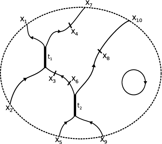
Our graphs are embedded in a disk and have two types of edges, unoriented and oriented. Unoriented edges are called “thick” and drawn accordingly; each vertex adjoining a thick edge has either two oriented edges leaving it or two entering. In figure 6 left x1,x2x_{1},x_{2} are outgoing and x3,x4x_{3},x_{4} are incoming. Oriented edges are allowed to have marks and we also allow closed loops; points of the boundary are also referred to as marks. See for example figure 4. To such a graph Γ\Gamma we assign a matrix factorization in the following manner:

Let

P⁡(x)=1n+1​xn+1+an−2n−1​xn−1+⋯+a12​x2+a0​x.P(x)=\frac{1}{n+1}x^{n+1}+\frac{a_{n-2}}{n-1}x^{n-1}+\dots+\frac{a_{1}}{2}x^{2}+a_{0}x.

Thick edges: To a thick edge tt as in figure 6 left we assign a factorization CtC_{t} with potential ωt=P⁡(x1)+P⁡(x2)−P⁡(x3)−P⁡(x4)\omega_{t}=P(x_{1})+P(x_{2})-P(x_{3})-P(x_{4}) over the ring Rt=ℚ⁡[a0,…,an−2]​[x1,x2,x3,x4]R_{t}=\mathbb{Q}[a_{0},\dots,a_{n-2}][x_{1},x_{2},x_{3},x_{4}].

Since xk+ykx^{k}+y^{k} lies in the ideal generated by x+yx+y and x​yxy we can write it as a polynomial gk​(x+y,x​y)g_{k}(x+y,xy). More explicitly,

gk​(s1,s2)=s1k+k​∑1≤i≤k2(−1)ii​(k−1−ii−1)​s2i​s1k−2​ig_{k}(s_{1},s_{2})=s_{1}^{k}+k\sum_{1\leq i\leq\frac{k}{2}}\frac{(-1)^{i}}{i}{{k-1-i}\choose{i-1}}s_{2}^{i}s_{1}^{k-2i}

Hence, x1k+x2k−x3k−x4kx_{1}^{k}+x_{2}^{k}-x_{3}^{k}-x_{4}^{k} can be written as

x1k+x2k−x3k−x4k=(x1+x2−x3−x4)​uk′+(x1​x2−x3​x4)​uk′′x_{1}^{k}+x_{2}^{k}-x_{3}^{k}-x_{4}^{k}=(x_{1}+x_{2}-x_{3}-x_{4})u_{k}^{\prime}+(x_{1}x_{2}-x_{3}x_{4})u_{k}^{\prime\prime}

where

uk′=x1k+x2k−gk​(x3+x4,x1​x2)x1+x2−x3−x4,u_{k}^{\prime}=\displaystyle\frac{x_{1}^{k}+x_{2}^{k}-g_{k}(x_{3}+x_{4},x_{1}x_{2})}{x_{1}+x_{2}-x_{3}-x_{4}},
uk′′=gk​(x3+x4,x1​x2)−x3k−x4kx1​x2−x3​x4.u_{k}^{\prime\prime}=\displaystyle\frac{g_{k}(x_{3}+x_{4},x_{1}x_{2})-x_{3}^{k}-x_{4}^{k}}{x_{1}x_{2}-x_{3}x_{4}}.

[Notice that our un+1′u_{n+1}^{\prime} and un+1′′u_{n+1}^{\prime\prime} are the same as the u1u_{1} and u2u_{2} in [13], respectively.]

Let

𝒰1=1n+1​un+1′+an−2n−1​un−1′+⋯+a12​u2′+a0,\mathcal{U}_{1}=\frac{1}{n+1}u_{n+1}^{\prime}+\frac{a_{n-2}}{n-1}u_{n-1}^{\prime}+\dots+\frac{a_{1}}{2}u_{2}^{\prime}+a_{0},

and

𝒰2=1n+1​un+1′′+an−2n−1​un−1′′+⋯+a12​u2′′.\mathcal{U}_{2}=\frac{1}{n+1}u_{n+1}^{\prime\prime}+\frac{a_{n-2}}{n-1}u_{n-1}^{\prime\prime}+\dots+\frac{a_{1}}{2}u_{2}^{\prime\prime}.

Define CtC_{t} to be the tensor product of graded factorizations

Rt→𝒰1Rt​{1−n}→x1+x2−x3−x4Rt,R_{t}\xrightarrow{\mathcal{U}_{1}}R_{t}\{1-n\}\xrightarrow{x_{1}+x_{2}-x_{3}-x_{4}}R_{t},

and

Rt→𝒰2Rt​{3−n}→x1​x2−x3​x4Rt,R_{t}\xrightarrow{\mathcal{U}_{2}}R_{t}\{3-n\}\xrightarrow{x_{1}x_{2}-x_{3}x_{4}}R_{t},

with the product shifted by {−1}\{-1\}.

Arcs: To an arc α\alpha bounded by marks oriented from jj to ii we assign the factorization LjiL_{j}^{i}

Rα→𝒫i​jRα→xi−xjRα,R_{\alpha}\xrightarrow{\mathcal{P}_{ij}}R_{\alpha}\xrightarrow{x_{i}-x_{j}}R_{\alpha},

where Rα=ℚ⁡[a0,…,an−2]​[xi,xj]R_{\alpha}=\mathbb{Q}[a_{0},\dots,a_{n-2}][x_{i},x_{j}] and

𝒫i​j=P⁡(xi)−P⁡(xj)xi−xj.\mathcal{P}_{ij}=\displaystyle\frac{P(x_{i})-P(x_{j})}{{x_{i}-x_{j}}}.

Finally, to an oriented loop with no marks we assign the complex 0→𝒜→0=𝒜​⟨1⟩0\rightarrow\mathcal{A}\rightarrow 0=\mathcal{A}\langle 1\rangle where 𝒜=ℚ⁡[a0,…,an−2]​[x]/(xn+an−2​xn−2+⋯+a1​x+a0)\mathcal{A}=\mathbb{Q}[a_{0},\dots,a_{n-2}][x]/(x^{n}+a_{n-2}x^{n-2}+\dots+a_{1}x+a_{0}). [Note: to a loop with marks we assign the tensor product of LjiL_{j}^{i}’s as above, but this turns out to be isomorphic to A​⟨1⟩A\langle 1\rangle in the homotopy category.]

Refer to caption

Figure 4: A planar graph

We define C⁡(Γ)C(\Gamma) to be the tensor product of CtC_{t} over all thick edges tt, LjiL^{i}_{j} over all edges α\alpha from jj to ii, and A​⟨1⟩A\langle 1\rangle over all oriented markless loops. This tensor product is taken over appropriate rings such that C⁡(Γ)C(\Gamma) is a free module over R=ℚ⁡[a0,…,an−2]​[{xi}]R=\mathbb{Q}[a_{0},\dots,a_{n-2}][\{x_{i}\}] where the xix_{i}’s are marks. For example, to the graph in figure 4 we assign C⁡(Γ)=L47⊗Ct1⊗L63⊗Ct2⊗L810⊗A⁡⟨1⟩C(\Gamma)=L^{7}_{4}\otimes C_{t_{1}}\otimes L^{3}_{6}\otimes C_{t_{2}}\otimes L^{10}_{8}\otimes A\langle 1\rangle tensored over ℚ⁡[a0,…,an−2]​[x4]\mathbb{Q}[a_{0},\dots,a_{n-2}][x_{4}], ℚ⁡[a0,…,an−2]​[x3]\mathbb{Q}[a_{0},\dots,a_{n-2}][x_{3}], ℚ⁡[a0,…,an−2]​[x6]\mathbb{Q}[a_{0},\dots,a_{n-2}][x_{6}], ℚ⁡[a0,…,an−2]​[x8]\mathbb{Q}[a_{0},\dots,a_{n-2}][x_{8}] and ℚ⁡[a0,…,an−2]\mathbb{Q}[a_{0},\dots,a_{n-2}] respectively. C⁡(Γ)C(\Gamma) becomes a ℤ⊕ℤ2\mathbb{Z}\oplus\mathbb{Z}_{2}-graded complex with the ℤ2\mathbb{Z}_{2}-grading coming from the matrix factorization. It has potential ω=∑i∈∂Γ±P(xi)\omega=\displaystyle\sum_{i\in\partial\Gamma}\pm P(x_{i}), where ∂Γ\partial\Gamma is the set of all boundary marks and the ++, −- is determined by whether the direction of the edge corresponding to xix_{i} is towards or away from the boundary. [Note: if Γ\Gamma is a closed graph the potential is zero and we have an honest 22-complex.]

Example: Let us look at the factorization assigned to an oriented loop with two marks xx and yy. We start out with the factorization LxyL_{x}^{y} assigned to an arc and then “close it off,” which corresponds to moding out by the ideal generated by the relation x=yx=y, see figure 5. We arrive at

R→xn+an−2​xn−2+⋯+a1​x+a0R→0R,R\xrightarrow{x^{n}+a_{n-2}x^{n-2}+\dots+a_{1}x+a_{0}}R\xrightarrow{0}R,

where R=ℚ⁡[a0,…,an−2]​[x]R=\mathbb{Q}[a_{0},\dots,a_{n-2}][x].

Refer to caption

Figure 5: “Closing off” an arc

The homology of this complex is supported in degree 11, with

H1​(Lxy/⟨x=y⟩)=ℚ⁡[a0,…,an−2]​[x]/(xn+an−2​xn−2+⋯+a1​x+a0).H^{1}(L_{x}^{y}/\langle x=y\rangle)=\mathbb{Q}[a_{0},\dots,a_{n-2}][x]/(x^{n}+a_{n-2}x^{n-2}+\dots+a_{1}x+a_{0}).

This is the algebra 𝒜\mathcal{A} we associated to an oriented loop with no marks. As we set out to define a homology theory that assigns to the unkot the U⁡(n)U(n)-equivariant cohomology of ℂ​ℙn−1\mathbb{CP}^{n-1}, this example illustrates the choice of potential P⁡(x)P(x). Notice that 𝒜\mathcal{A} has a natural Frobenius algebra structure with trace map ε\varepsilon and unit map ι\iota.

ε:ℚ⁡[a0,…,an−2]​[x]/(xn+an−2​xn−2+⋯+a1​x+a0)⟶ℚ⁡[a0,…,an−2],\varepsilon:\mathbb{Q}[a_{0},\dots,a_{n-2}][x]/(x^{n}+a_{n-2}x^{n-2}+\dots+a_{1}x+a_{0})\longrightarrow\mathbb{Q}[a_{0},\dots,a_{n-2}],

given by

ε⁡(xn−1)=1;ε⁡(xi)=0,i≤n−2,\varepsilon(x^{n-1})=1;\ \ \varepsilon(x^{i})=0,\ i\leq n-2,

and

ι:ℚ⁡[a0,…,an−2]⟶ℚ⁡[a0,…,an−2]​[x]/(xn+an−2​xn−2+⋯+a1​x+a0),\iota:\mathbb{Q}[a_{0},\dots,a_{n-2}]\longrightarrow\mathbb{Q}[a_{0},\dots,a_{n-2}][x]/(x^{n}+a_{n-2}x^{n-2}+\dots+a_{1}x+a_{0}),
ι⁡(1)=1.\iota(1)=1.

Notice that ε⁡(xi)\varepsilon(x^{i}) is not equal to zero for i≥ni\geq n but a homogeneous polynomial in the aia_{i}’s. Many of the calculations in [13] necessary for the proofs of invariance would fail due to this fact; proposition 44 will be key in getting around this difference. Of course, setting ai=0a_{i}=0, for all ii, gives us the same Frobenius algebra, unit and trace maps as in [13].

Refer to caption

Figure 6: Maps χ0\chi_{0} and χ1\chi_{1}

The maps χ0\chi_{0} and χ1\chi_{1}: We now define maps between matrix factorizations associated to a thick edge and two disjoint arcs as in figure 6. Let Γ0\Gamma^{0} correspond to the two disjoint arcs and Γ1\Gamma^{1} to the thick edge.

C⁡(Γ0)C(\Gamma^{0}) is the tensor product of L41L_{4}^{1} and L32L_{3}^{2}. If we assign labels aa, bb to L41L_{4}^{1}, L32L_{3}^{2} respectively, the tensor product can be written as

(R⁡(∅)R⁡(a​b)​{2−2​n})⟶P0(R⁡(a)​{1−n}R⁡(b)​{1−n})⟶P1(R⁡(∅)R⁡(a​b)​{2−2​n}),\left(\begin{array}[]{clcr}R(\varnothing)\\ R(ab)\{2-2n\}\end{array}\right)\stackrel{{\scriptstyle P_{0}}}{{\longrightarrow}}\left(\begin{array}[]{clcr}R(a)\{1-n\}\\ R(b)\{1-n\}\end{array}\right)\stackrel{{\scriptstyle P_{1}}}{{\longrightarrow}}\left(\begin{array}[]{clcr}R(\varnothing)\\ R(ab)\{2-2n\}\end{array}\right),

where

P0=(𝒫14x2−x3𝒫23x4−x1),P1=(x1−x4x2−x3𝒫23−𝒫14),P_{0}=\left(\begin{array}[]{cclcr}\mathcal{P}_{14}&x_{2}-x_{3}\\ \mathcal{P}_{23}&x_{4}-x_{1}\end{array}\right),\ \ P_{1}=\left(\begin{array}[]{cclcr}x_{1}-x_{4}&x_{2}-x_{3}\\ \mathcal{P}_{23}&-\mathcal{P}_{14}\end{array}\right),

and R=ℚ⁡[a0,…,an−2]​[x1,x2,x3,x4]R=\mathbb{Q}[a_{0},\dots,a_{n-2}][x_{1},x_{2},x_{3},x_{4}].

Assigning labels a′a^{\prime} and b′b^{\prime} to the two factorizations in C⁡(Γ1)C(\Gamma^{1}), we have that C⁡(Γ1)C(\Gamma^{1}) is given by

(R⁡(∅)​{−1}R⁡(a′​b′)​{3−2​n})⟶Q0(R⁡(a′)​{−n}R⁡(b′)​{2−n})⟶Q1(R⁡(∅)​{−1}R⁡(a′​b′)​{3−2​n}),\left(\begin{array}[]{clcr}R(\varnothing)\{-1\}\\ R(a^{\prime}b^{\prime})\{3-2n\}\end{array}\right)\stackrel{{\scriptstyle Q_{0}}}{{\longrightarrow}}\left(\begin{array}[]{clcr}R(a^{\prime})\{-n\}\\ R(b^{\prime})\{2-n\}\end{array}\right)\stackrel{{\scriptstyle Q_{1}}}{{\longrightarrow}}\left(\begin{array}[]{clcr}R(\varnothing)\{-1\}\\ R(a^{\prime}b^{\prime})\{3-2n\}\end{array}\right),

where

Q0=(𝒰1x1​x2−x3​x4𝒰2x3+x4−x1−x2),Q1=(x1+x2−x3−x4x1​x2−x3​x4𝒰2−𝒰1).Q_{0}=\left(\begin{array}[]{cclcr}\mathcal{U}_{1}&x_{1}x_{2}-x_{3}x_{4}\\ \mathcal{U}_{2}&x_{3}+x_{4}-x_{1}-x_{2}\end{array}\right),\ \ Q_{1}=\left(\begin{array}[]{cclcr}x_{1}+x_{2}-x_{3}-x_{4}&x_{1}x_{2}-x_{3}x_{4}\\ \mathcal{U}_{2}&-\mathcal{U}_{1}\end{array}\right).

A map between C⁡(Γ0)C(\Gamma^{0}) and C⁡(Γ1)C(\Gamma^{1}) can be given by a pair of 2×22\times 2 matrices. Define χ0:C⁡(Γ0)→C⁡(Γ1)\chi_{0}:C(\Gamma^{0})\rightarrow C(\Gamma^{1}) by

U0=(x4−x2+μ⁡(x1+x2−x3−x4)0k11),U1=(x4+μ⁡(x1−x4)μ⁡(x2−x3)−x2−11),U_{0}=\left(\begin{array}[]{cclcr}x_{4}-x_{2}+\mu(x_{1}+x_{2}-x_{3}-x_{4})&0\\ k_{1}&1\end{array}\right),\ U_{1}=\left(\begin{array}[]{cclcr}x_{4}+\mu(x_{1}-x_{4})&\mu(x_{2}-x_{3})-x_{2}\\ -1&1\end{array}\right),

where

k1=(μ−1)​𝒰2+𝒰1+x1​𝒰2−𝒫23x1−x4,f​o​r​μ∈ℤk_{1}=(\mu-1)\mathcal{U}_{2}+\frac{\mathcal{U}_{1}+x_{1}\mathcal{U}_{2}-\mathcal{P}_{23}}{x_{1}-x_{4}},\ for\ \mu\in\mathbb{Z}

and χ1:C⁡(Γ1)→C⁡(Γ0)\chi_{1}:C(\Gamma^{1})\rightarrow C(\Gamma^{0}) by

V0=(10k2k3),V1=(1x3+λ⁡(x2−x3)1x1+λ⁡(x4−x1)).V_{0}=\left(\begin{array}[]{cclcr}1&0\\ k_{2}&k_{3}\end{array}\right),\ \ V_{1}=\left(\begin{array}[]{cclcr}1&x_{3}+\lambda(x_{2}-x_{3})\\ 1&x_{1}+\lambda(x_{4}-x_{1})\end{array}\right).

where

k2=λ​𝒰2+𝒰1+x1​𝒰2−𝒫23x4−x1,k3=λ⁡(x3+x4−x1−x2)+x1−x3,f​o​r​λ∈ℤ.k_{2}=\lambda\mathcal{U}_{2}+\frac{\mathcal{U}_{1}+x_{1}\mathcal{U}_{2}-\mathcal{P}_{23}}{x_{4}-x_{1}},\ k_{3}=\lambda(x_{3}+x_{4}-x_{1}-x_{2})+x_{1}-x_{3},\ for\ \lambda\in\mathbb{Z}.

It is easy to see that different choices of μ\mu and λ\lambda give homotopic maps. These maps are degree 11. We encourage the reader to compare the above factorizations and maps to that of [13], and notice the difference stemming from the fact that here we are working with new potentials.

Just like in [13] we specialize to λ=0\lambda=0 and μ=1\mu=1, and compute to see that the composition χ1​χ0=(x1−x3)​I\chi_{1}\chi_{0}=(x_{1}-x_{3})I, where II is the identity matrix, i.e. χ1​χ0\chi_{1}\chi_{0} is multiplication by x1−x3x_{1}-x_{3}, which is homotopic to multiplication by x4−x2x_{4}-x_{2} as an endomorphism of C⁡(Γ0)C(\Gamma^{0}). Similarly χ0​χ1=(x1−x3)​I\chi_{0}\chi_{1}=(x_{1}-x_{3})I, which is also homotopic to multiplication by x4−x2x_{4}-x_{2} as an endomorphism of C⁡(Γ1)C(\Gamma^{1}).

Direct Sum Decomposition 0

Refer to caption

Figure 7: DSD 00

where D0=∑i=0n−1xi​ιD_{0}=\displaystyle\sum_{i=0}^{n-1}x^{i}\iota and D0−1=∑i=0n−1ε​xn−1−i.D_{0}^{-1}=\displaystyle\sum_{i=0}^{n-1}\varepsilon x^{n-1-i}.

By the pictures above, we really mean the complexes assigned to them, i.e. ∅​⟨1⟩\emptyset\langle 1\rangle is the complex with ℚ⁡[a0,…,an−2]\mathbb{Q}[a_{0},\dots,a_{n-2}] sitting in homological grading 11 and the unknot is the complex 𝒜​⟨1⟩\mathcal{A}\langle 1\rangle as before. The map ε​xi\varepsilon x^{i} is a composition of maps

𝒜⁡⟨1⟩→xi𝒜⁡⟨1⟩→𝜀∅​⟨1⟩,\mathcal{A}\langle 1\rangle\xrightarrow{x^{i}}\mathcal{A}\langle 1\rangle\xrightarrow{\varepsilon}\emptyset\langle 1\rangle,

where xix^{i} is multiplication and ε\varepsilon is the trace map.

The map xi​ιx^{i}\iota is analogous. It is easy to check that the above maps are grading preserving and their composition is an isomorphism in the homotopy category. □\square

Direct Sum Decomposition I We follow [13] closely. Recall that here matrix factorizations are over the ring R=ℚ⁡[a0,…,an−2]R=\mathbb{Q}[a_{0},\dots,a_{n-2}].

Refer to caption

Figure 8: DSD I
Proposition 10.

The following two factorizations are isomorphic in h​m​fωhmf_{\omega}.

C⁡(Γ)≅∑i=0n−2C⁡(Γ1)​⟨1⟩​{2−n+2​i}.C(\Gamma)\cong\sum_{i=0}^{n-2}C(\Gamma_{1})\langle 1\rangle\{2-n+2i\}.

Proof: Define grading preserving maps αi\alpha_{i} and βi\beta_{i} for 0≤i≤n−20\leq i\leq n-2, as in [13],

αi:C⁡(Γ1)​⟨1⟩⟶C⁡(Γ)​{n−2−2​i},\alpha_{i}\ :\ C(\Gamma_{1})\langle 1\rangle\longrightarrow C(\Gamma)\{n-2-2i\},
αi=∑j=0ix1j​x2i−j​α,\alpha_{i}\ =\ \sum_{j=0}^{i}x_{1}^{j}x_{2}^{i-j}\alpha,

where α=χ0∘ι′\alpha=\chi_{0}\circ\iota^{\prime} is defined to be the composition in figure 9. [ι′=ι⊗I​d\iota^{\prime}=\iota\otimes Id where I​dId corresponds to the inclusion of the arc Γ1\Gamma_{1} into the disjoint union of the arc and circle, and ι\iota is the unit map.]

βi:C⁡(Γ)​{n−2−2​i}⟶C⁡(Γ1)​⟨1⟩,\beta_{i}\ :\ C(\Gamma)\{n-2-2i\}\longrightarrow C(\Gamma_{1})\langle 1\rangle,
βi=β​x1n−i−2,\beta_{i}\ =\ \beta x_{1}^{n-i-2},

where β=ε′∘χ1\beta=\varepsilon^{\prime}\circ\chi_{1}, see figure 10. [Similarly, ε′=ε⊗I​d\varepsilon^{\prime}=\varepsilon\otimes Id.]

Refer to caption

Figure 9: The map α\alpha

Refer to caption

Figure 10: The map β\beta

Define maps:

α′=∑i=0n−2αi:∑i=0n−2C⁡(Γ1)​⟨1⟩​{2−n+2​i}⟶C⁡(Γ),\alpha^{\prime}=\sum_{i=0}^{n-2}\alpha_{i}\ :\ \sum_{i=0}^{n-2}C(\Gamma_{1})\langle 1\rangle\{2-n+2i\}\longrightarrow C(\Gamma),

and

β′=∑i=0n−2βi:C⁡(Γ)⟶C⁡(Γ1)​⟨1⟩​{2−n+2​i}.\beta^{\prime}=\sum_{i=0}^{n-2}\beta_{i}\ :\ C(\Gamma)\longrightarrow C(\Gamma_{1})\langle 1\rangle\{2-n+2i\}.

In [13] it was shown that these maps are isomorphisms of factorizations over the ring R¯=ℚ⁡[x1,x2,x3,x4]\overline{R}=\mathbb{Q}[x_{1},x_{2},x_{3},x_{4}]. By Proposition 7 we are done.□\square

Direct Sum Decomposition II

Refer to caption

Figure 11: DSD II
Proposition 11.

There is an isomorphism of factorizations in h​m​fωhmf_{\omega}

C⁡(Γ)≅C⁡(Γ1)​{1}⊕C⁡(Γ1)​{−1}.C(\Gamma)\cong C(\Gamma_{1})\{1\}\oplus C(\Gamma_{1})\{-1\}.

Proof: See [13].□\square

Direct Sum Decomposition III

Refer to caption

Figure 12: DSD III
Proposition 12.

There is an isomorphism of factorizations in h​m​fωhmf_{\omega}

C(Γ)≅C(Γ2)⊕(⊕i=0n−3C(Γ1)⟨1⟩{3−n+2i}).C(\Gamma)\cong C(\Gamma_{2})\oplus\left(\oplus_{i=0}^{n-3}C(\Gamma_{1})\langle 1\rangle\{3-n+2i\}\right).

Proof: Define grading preserving maps αi\alpha_{i}, βi\beta_{i} for 0≤i≤n−30\leq i\leq n-3

αi:C⁡(Γ1)​⟨1⟩​{3−n+2​i}⟶C⁡(Γ)\alpha_{i}\ :\ C(\Gamma_{1})\langle 1\rangle\{3-n+2i\}\longrightarrow C(\Gamma)
αi=x5​α,\alpha_{i}\ =\ x_{5}\alpha,

where α=χ0′∘ι′\alpha=\chi_{0}^{\prime}\circ\iota^{\prime}, ι′=I​d⊗ι⊗I​d\iota^{\prime}=Id\otimes\iota\otimes Id with identity maps on the two arcs, and χ0′\chi_{0}^{\prime} the composition of two χ0\chi_{0}’s corresponding to merging the two arcs into the circle, see figure 13.

Refer to caption

Figure 13: The map α\alpha
βi:C⁡(Γ)⟶C⁡(Γ1)​⟨1⟩​{3−n+2​i}\beta_{i}\ :\ C(\Gamma)\longrightarrow C(\Gamma_{1})\langle 1\rangle\{3-n+2i\}
βi=∑i=0n−3β​∑a+b+c=n−3−ix2a​x4b​x1c,\beta_{i}\ =\ \displaystyle\sum_{i=0}^{n-3}\beta\sum_{a+b+c=n-3-i}x_{2}^{a}x_{4}^{b}x_{1}^{c},

where β\beta is defined as in figure 14.

Refer to caption

Figure 14: The map β\beta
S:C⁡(Γ)⟶C⁡(Γ2).S:C(\Gamma)\longrightarrow C(\Gamma_{2}).

In addition, let SS be the map gotten by “merging” the thick edges together to form two disjoint horizontal arcs, as in the top righ-hand corner above; an exact description of SS won’t really matter so we will not go into details and refer the interested reader to [13].

Let α′=∑i=0n−3αi\alpha^{\prime}=\sum_{i=0}^{n-3}\alpha_{i} and β′=∑i=0n−3βi\beta^{\prime}=\sum_{i=0}^{n-3}\beta_{i}. In [13] it shown that S⊕β′S\oplus\beta^{\prime} is an isomorphism in h​m​fωhmf_{\omega}, with inverse S−1⊕α′S^{-1}\oplus\alpha^{\prime}, so by Proposition 7 we are done. □\square.

[Note: we abuse notation throughout by using a direct sum of maps to indicate a map to or from a direct summand.]

Direct Sum Decomposition IV

Refer to caption

Figure 15: The factorizations in DSD IV
Proposition 13.

There is an isomorphism in h​m​fωhmf_{\omega}

C⁡(Γ1)⊕C⁡(Γ2)≅C⁡(Γ3)⊕C⁡(Γ4).C(\Gamma_{1})\oplus C(\Gamma_{2})\cong C(\Gamma_{3})\oplus C(\Gamma_{4}).

Proof: Notice that C⁡(Γ1)C(\Gamma_{1}) turns into C⁡(Γ3)C(\Gamma_{3}) if we permute x1x_{1} with x3x_{3}, and C⁡(Γ2)C(\Gamma_{2}) turns into C⁡(Γ4)C(\Gamma_{4}) if we permute x2x_{2} and x4x_{4}. The proposition is proved by introducing a new factorization Υ\Upsilon that is invariant under these permutations and showing that C⁡(Γ1)≅Υ⊕C⁡(Γ4)C(\Gamma_{1})\cong\Upsilon\oplus C(\Gamma_{4}), and C⁡(Γ3)≅Υ⊕C⁡(Γ2)C(\Gamma_{3})\cong\Upsilon\oplus C(\Gamma_{2}). Since these decompositions hold for matrix factorizations over the ring R¯=ℚ⁡[x1,…,x6]\overline{R}=\mathbb{Q}[x_{1},\dots,x_{6}], they hold here as well. We refer the reader to [13] for details. □\square

3 Tangles and complexes

By a tangle TT we mean an oriented, closed one manifold embedded in the unit ball 𝔹3\mathbb{B}^{3}, with boundary points of TT lying on the equator of the bounding sphere 𝕊2\mathbb{S}^{2}. An isotopy of tangles preserves the boundary points. A diagram DD for TT is a generic projection of TT onto the plane of the equator.

Refer to caption

Figure 16: Complexes associated to pos/neg crossings; the numbers below the diagrams are cohomological degrees.

Given such a diagram DD and a crossing pp of DD we resolve it in two ways, depending on whether the crossing is positive or negative, and assign to pp the corresponding complex CpC^{p}, see figure 16 . We define C⁡(D)C(D) to be the comples of matrix factorizations which is the tensor product of CpC^{p}, over all crossings pp, of LjiL_{j}^{i} over arcs j→ij\rightarrow i, and of 𝒜​⟨1⟩\mathcal{A}\langle 1\rangle over all crossingless markless circles in DD. The tensor product is taken over appropriate polynomial rings, so that C⁡(D)C(D) is free and of finite rank as an RR-module, where R=ℚ⁡[a0,…,an−2]​[x1,…,xk]R=\mathbb{Q}[a_{0},\dots,a_{n-2}][x_{1},\dots,x_{k}], and the xix_{i}’s are on the boundary of DD. This complex is ℤ⊕ℤ⊕ℤ2\mathbb{Z}\oplus\mathbb{Z}\oplus\mathbb{Z}_{2} graded.

For example, the complex associated to the tangle in figure 17 is gotten by first tensoring Cp1C^{p_{1}} with Cp2C^{p_{2}} over the ring ℚ⁡[a0,…,an−2]​[x3,x4]\mathbb{Q}[a_{0},\dots,a_{n-2}][x_{3},x_{4}], then tensoring Cp1⊗Cp2C^{p_{1}}\otimes C^{p_{2}} with L12L_{1}^{2} over ℚ⁡[a0,…,an−2]​[x2]\mathbb{Q}[a_{0},\dots,a_{n-2}][x_{2}], and finally tensoring Cp1⊗Cp2⊗L12C^{p_{1}}\otimes C^{p_{2}}\otimes L_{1}^{2} with 𝒜​⟨1⟩\mathcal{A}\langle 1\rangle over ℚ⁡[a0,…,an−2]\mathbb{Q}[a_{0},\dots,a_{n-2}].

Refer to caption

Figure 17: Diagram of a tangle
Theorem 14.

If DD and D′D^{\prime} are two diagrams representing the same tangle TT, then C⁡(D)C(D) and C⁡(D′)C(D^{\prime}) are isomorphic modulo homotopy in the homotopy category h​m​fωhmf_{\omega}, i.e. the isomorphism class of C⁡(D)C(D) is an invariant of TT.

The proof of this statement involves checking the invariance under the Reidemeister moves to which the next section is devoted.

Link Homology When the tangle in question is a link LL, i.e. there are no boundary points and R=ℚ⁡[a0,…,an−2]R=\mathbb{Q}[a_{0},\dots,a_{n-2}], complexes of matrix factorizations associated to each resolution have non-trivial cohomology only in one degree (in the cyclic degree which is the number of components of LL modulo 22). The grading of the cohomology of C⁡(L)C(L) reduces to ℤ⊕ℤ\mathbb{Z}\oplus\mathbb{Z}. We denote the resulting cohomology groups of the complex C⁡(L)C(L) by

Hn(L)=⊕i,j∈ℤHni,j(L),H_{n}(L)=\oplus_{i,j\in\mathbb{Z}}H^{i,j}_{n}(L),

and the Euler characteristic by

Pn​(L)=∑i,j∈ℤ(−1)i​qj​d​i​mR​Hni,j​(L).P_{n}(L)=\sum_{i,j\in\mathbb{Z}}(-1)^{i}q^{j}dim_{R}H^{i,j}_{n}(L).

It is clear from the construction that

Corollary 15.

Setting the aia_{i}’s to zero in the chain complex we arrive at the Khovanov-Rozansky homology, with Euler characteristic the quantum s​lnsl_{n}-polynomial of LL.

4 Invariance under the Reidemeister moves

Refer to caption

Figure 18:

R1: To the tangle in figure 18 left we associate the following complex

0\textstyle{0\ignorespaces\ignorespaces\ignorespaces\ignorespaces}C⁡(Γ1)​{1−n}\textstyle{C(\Gamma_{1})\{1-n\}\ignorespaces\ignorespaces\ignorespaces\ignorespaces}χ0\scriptstyle{\chi_{0}}C⁡(Γ2)​{−n}\textstyle{C(\Gamma_{2})\{-n\}\ignorespaces\ignorespaces\ignorespaces\ignorespaces}0.\textstyle{0.}

Refer to caption

Figure 19: Reidemeister 1 complex

Using direct decompositions 00 and I, and for a moment forgoing the overall grading shifts, we see that this complex is isomorphic to

0\textstyle{0\ignorespaces\ignorespaces\ignorespaces\ignorespaces}⨁i=0n−1C⁡(Γ)​{1−n+2​i}\textstyle{\bigoplus_{i=0}^{n-1}C(\Gamma)\{1-n+2i\}\ignorespaces\ignorespaces\ignorespaces\ignorespaces}Φ\scriptstyle{\Phi}⨁j=0n−2C⁡(Γ)​{1+n−2​j}\textstyle{\bigoplus_{j=0}^{n-2}C(\Gamma)\{1+n-2j\}\ignorespaces\ignorespaces\ignorespaces\ignorespaces}0,\textstyle{0,}

where

Φ=β′∘χ0∘∑i=0n−1x1i​ι′=(∑j=0n−2ε′∘χ1​x1n−j−2)∘χ0∘∑i=0n−1x1i​ι′=∑i=0n−1∑j=0n−2ε′∘χ1∘χ0​x1n−j+i−2∘ι′=∑i=0n−1∑j=0n−2ε′​(x1−x2)​x1n−j+i−2∘ι′=ε′​(∑i=0n−1∑j=0n−2(x1n−j+i−1−x2​x1n−j+i−2))​ι′.\begin{array}[]{rcl}\Phi&=&\beta^{\prime}\circ\chi_{0}\circ\displaystyle\sum_{i=0}^{n-1}x_{1}^{i}\iota^{\prime}\\ &=&\big(\displaystyle\sum_{j=0}^{n-2}\varepsilon^{\prime}\circ\chi_{1}x_{1}^{n-j-2}\big)\circ\chi_{0}\circ\displaystyle\sum_{i=0}^{n-1}x_{1}^{i}\iota^{\prime}\\ &=&\displaystyle\sum_{i=0}^{n-1}\displaystyle\sum_{j=0}^{n-2}\varepsilon^{\prime}\circ\chi_{1}\circ\chi_{0}x_{1}^{n-j+i-2}\circ\iota^{\prime}\\ &=&\displaystyle\sum_{i=0}^{n-1}\displaystyle\sum_{j=0}^{n-2}\varepsilon^{\prime}(x_{1}-x_{2})x_{1}^{n-j+i-2}\circ\iota^{\prime}\\ &=&\varepsilon^{\prime}\big(\displaystyle\sum_{i=0}^{n-1}\displaystyle\sum_{j=0}^{n-2}(x_{1}^{n-j+i-1}-x_{2}x_{1}^{n-j+i-2})\big)\iota^{\prime}.\\ \end{array}

Hence, Φ\Phi is an upper triangular matrix with 11’s on the diagonal, which implies that up to homotopy the above complexes are isomorphic to

0⟶C⁡(Γ)​{n−1}⟶0.0\longrightarrow C(\Gamma)\{n-1\}\longrightarrow 0.

Recalling that we left out the overall grading shift of {−n+1}\{-n+1\} we arrive at the desired conclusion:

0\textstyle{0\ignorespaces\ignorespaces\ignorespaces\ignorespaces}C⁡(Γ1)​{1−n}\textstyle{C(\Gamma_{1})\{1-n\}\ignorespaces\ignorespaces\ignorespaces\ignorespaces}χ0\scriptstyle{\chi_{0}}C⁡(Γ2)​{−n}\textstyle{C(\Gamma_{2})\{-n\}\ignorespaces\ignorespaces\ignorespaces\ignorespaces}0\textstyle{0}

is homotopic to

0⟶C⁡(Γ)​{n−1}⟶0.0\longrightarrow C(\Gamma)\{n-1\}\longrightarrow 0.

The other Reidemeister 11 move is proved analogously. □\square

R2: The complex associated to the tangle in figure 20 left is

Refer to caption

Figure 20:
0⟶C⁡(Γ00)​{1}→(f1,f3)tC⁡(Γ01)⊕C⁡(Γ10)→(f2,−f4)C⁡(Γ11)​{−1}⟶0.0\longrightarrow C(\Gamma_{00})\{1\}\xrightarrow{(f_{1},f_{3})^{t}}\begin{array}[]{c}C(\Gamma_{01})\\ \oplus\\ C(\Gamma_{10})\end{array}\xrightarrow{(f_{2},-f_{4})}C(\Gamma_{11})\{-1\}\longrightarrow 0.

Refer to caption

Figure 21: Reidemeister 2a complex

Using direct decomposition II we know that

C⁡(Γ10)≅C⁡(Γ1)​{1}⊕C⁡(Γ1)​{−1}.C(\Gamma_{10})\cong C(\Gamma_{1})\{1\}\oplus C(\Gamma_{1})\{-1\}.

Hence, the above complex is isomorphic to

0⟶C⁡(Γ00)​{1}→(f1,f03,f13)tC⁡(Γ01)⊕C⁡(Γ1)​{1}⊕C⁡(Γ1)​{−1}→(f2,−f04,−f14)C⁡(Γ11)​{−1}⟶0,0\longrightarrow C(\Gamma_{00})\{1\}\xrightarrow{(f_{1},f_{03},f_{13})^{t}}\begin{array}[]{c}C(\Gamma_{01})\\ \oplus\\ C(\Gamma_{1})\{1\}\\ \oplus\\ C(\Gamma_{1})\{-1\}\end{array}\xrightarrow{(f_{2},-f_{04},-f_{14})}C(\Gamma_{11})\{-1\}\longrightarrow 0,

where f03f_{03}, f13f_{13}, f04f_{04}, f14f_{14} are the degreee 00 maps that give the isomorphism of decomposition II. If we know that both f14f_{14} and f03f_{03} are isomorphisms then the subcomplex containing C⁡(Γ00),C⁡(Γ10)C(\Gamma_{00}),C(\Gamma_{10}), and C⁡(Γ11)C(\Gamma_{11}) is acyclic; moding out produces a complex homotopic to

0⟶C⁡(Γ0)⟶0.0\longrightarrow C(\Gamma_{0})\longrightarrow 0.

The next two lemmas establish the fact that f14f_{14} and f03f_{03} are indeed isomorphisms.

Lemma 16.

The space of degree 00 endomorphisms of C⁡(Γ1)C(\Gamma_{1}) is isomorphic to ℚ\mathbb{Q}. The space of degree 22 endomorphism is 33-dimensional spanned by x1,x2,x3,x4x_{1},x_{2},x_{3},x_{4} with only relation being x1+x2−x3−x4=0x_{1}+x_{2}-x_{3}-x_{4}=0 for n>2n>2, and 22-dimensional with the relations x1+x2=0x_{1}+x_{2}=0 and x3+x4=0x_{3}+x_{4}=0 for n=2n=2.

Proof: The complex H​o​m​(C⁡(Γ1),C⁡(Γ1))Hom(C(\Gamma_{1}),C(\Gamma_{1})) is isomorphic to the factorization of the pair (𝐛,𝐜)(\mathbf{b},\mathbf{c}) where

𝐛=(x1+x2+x3+x4,x1​x2−x3​x4,−𝒰1,−𝒰2),𝐜=(𝒰1,𝒰2,x1+x2+x3+x4,x1​x2−x3​x4).\mathbf{b}=(x_{1}+x_{2}+x_{3}+x_{4},x_{1}x_{2}-x_{3}x_{4},-\mathcal{U}_{1},-\mathcal{U}_{2}),\ \mathbf{c}=(\mathcal{U}_{1},\mathcal{U}_{2},x_{1}+x_{2}+x_{3}+x_{4},x_{1}x_{2}-x_{3}x_{4}).

The pair (𝐛,𝐜)(\mathbf{b},\mathbf{c}) is orthogonal, since this is a complex, and it is easy to see that the sequence 𝐜\mathbf{c} is regular (𝐜\mathbf{c} is certainly regular when we set the aia_{i}’s equal to zero) and hence the cohomology of this 22-complex is

ℚ⁡[a0,…,an−2]​[x1,x2,x3,x4]/(x1+x2+x3+x4,x1​x2−x3​x4,𝒰1,𝒰2).\mathbb{Q}[a_{0},\dots,a_{n-2}][x_{1},x_{2},x_{3},x_{4}]/(x_{1}+x_{2}+x_{3}+x_{4},x_{1}x_{2}-x_{3}x_{4},\mathcal{U}_{1},\mathcal{U}_{2}).

For n>2n>2 the last three terms of the above sequence are at least quadratic and, hence, have degree at least 44 (recall that deg⁡ai≥4\deg{a_{i}}\geq 4 for all ii). For n=2n=2, 𝒰2=u2′′\mathcal{U}_{2}=u_{2}^{\prime\prime} which is linear and we get the relations x1+x2=0x_{1}+x_{2}=0, x3+x4=0x_{3}+x_{4}=0. □\square

Lemma 17.

f14≠0f_{14}\neq 0 and f03≠0f_{03}\neq 0.

Proof: With the above lemma the proof follows the lines of [13]. □\square

Hence, f14f_{14} and f03f_{03} are indeed isomorphisms and we arrive at the desired conclusion.□\square

Refer to caption

Figure 22:

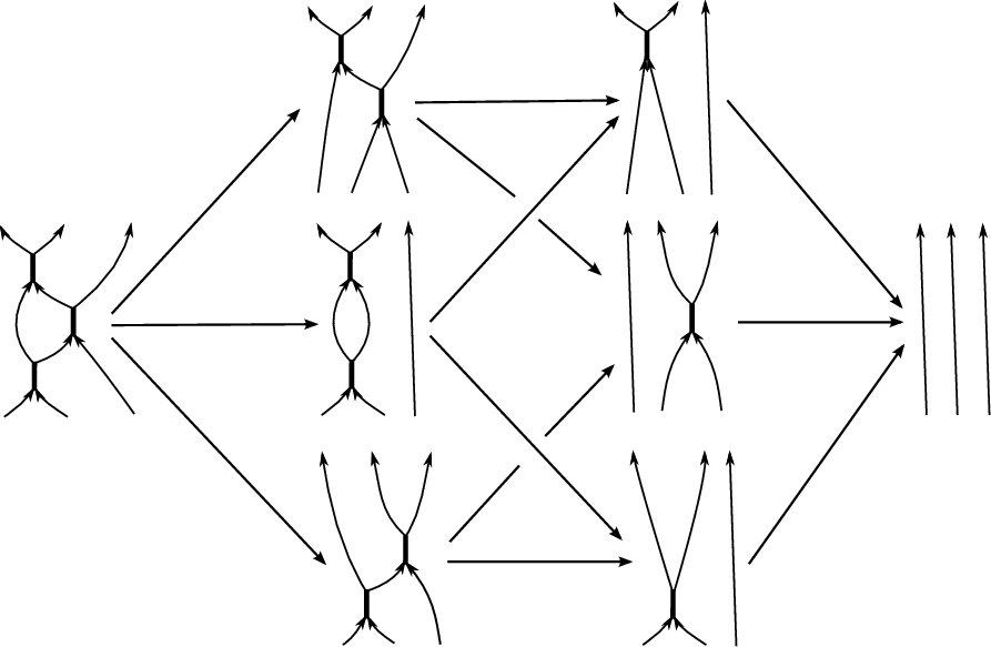
R3: The complex assigned to the tangle on the left-hand side of figure 22 is
Refer to caption

Figure 23: Reidemeister 3 complex
0⟶C⁡(Γ111)→d−3C⁡(Γ011)​{−1}⊕C⁡(Γ101)​{−1}⊕C⁡(Γ110)​{−1}→d−2C⁡(Γ100)​{−2}⊕C⁡(Γ010)​{−2}⊕C⁡(Γ001)​{−2}→d−1C⁡(Γ000)​{−3}⟶0.0\longrightarrow C(\Gamma_{111})\xrightarrow{d^{-3}}\begin{array}[]{c}C(\Gamma_{011})\{-1\}\\ \oplus\\ C(\Gamma_{101})\{-1\}\\ \oplus\\ C(\Gamma_{110})\{-1\}\end{array}\xrightarrow{d^{-2}}\begin{array}[]{c}C(\Gamma_{100})\{-2\}\\ \oplus\\ C(\Gamma_{010})\{-2\}\\ \oplus\\ C(\Gamma_{001})\{-2\}\end{array}\xrightarrow{d^{-1}}C(\Gamma_{000})\{-3\}\longrightarrow 0.

Direct sum decompositions II and III show that

C⁡(Γ101)≅C⁡(Γ100)​{1}⊕C⁡(Γ100)​{−1},C(\Gamma_{101})\cong C(\Gamma_{100})\{1\}\oplus C(\Gamma_{100})\{-1\},

and

C⁡(Γ111)≅C⁡(Γ100)⊕Υ.C(\Gamma_{111})\cong C(\Gamma_{100})\oplus\Upsilon.

Inserting these and using arguments analogous to those used in the decomposition proofs we reduce the original complex to
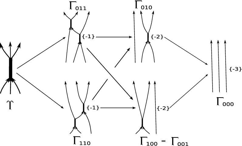
0⟶Υ→d−3C⁡(Γ011)​{−1}⊕C⁡(Γ110)​{−1}→d−2C⁡(Γ010)​{−2}⊕C⁡(Γ100)​{−2}→d−1C⁡(Γ000)​{−3}⟶0.0\longrightarrow\Upsilon\xrightarrow{d^{-3}}\begin{array}[]{c}C(\Gamma_{011})\{-1\}\\ \oplus\\ C(\Gamma_{110})\{-1\}\end{array}\xrightarrow{d^{-2}}\begin{array}[]{c}C(\Gamma_{010})\{-2\}\\ \oplus\\ C(\Gamma_{100})\{-2\}\end{array}\xrightarrow{d^{-1}}C(\Gamma_{000})\{-3\}\longrightarrow 0.

Refer to caption

Figure 24: Reidemeister 3 complex reduced
Proposition 18.

Assume n>2n>2, then for every arrow in 24 from object AA to BB the space of grading-preserving morphisms

H​o​mh​m​f​(C⁡(A),C⁡(B)​{−1})Hom_{hmf}(C(A),C(B)\{-1\})

is one dimensional. Moreover, the composition of any two arrows C⁡(A)⟶C⁡(B)​{−1}⟶C⁡(C)​{−2}C(A)\longrightarrow C(B)\{-1\}\longrightarrow C(C)\{-2\} is nonzero.

Proof: Once again the maps in question are all of degree ≤2\leq 2, and noticing that these remain nonzero when we work over the ring ℚ⁡[a0,…,an−2]\mathbb{Q}[a_{0},\dots,a_{n-2}], we can revert to the calculations in [13].□\square

Hence, this complex is invariant under the “flip” which takes x1x_{1} to x3x_{3} and x4x_{4} to x6x_{6}. This flip takes the complex associated to the braid on the left-hand side of figure 22 to the one on the right-hand side.□\square

5 Remarks

Given a diagram DD of a link LL let Cn​(D)C_{n}(D) be the equivariant s​lnsl_{n} chain complex constructed above. The homotopy class of Cn​(D)C_{n}(D) is an invariant of LL and consists of free ℚ⁡[a0,…,an−2]\mathbb{Q}[a_{0},\dots,a_{n-2}]-modules where the aia_{i}’s are coefficients with deg⁡(ai)=2​(n−i)\deg(a_{i})=2(n-i). The cohomology of this complex Hn​(D)H_{n}(D) is a graded ℚ⁡[a0,…,an−2]\mathbb{Q}[a_{0},\dots,a_{n-2}]-module. For a moment, let us consider the case where all the ai=0a_{i}=0 for 1≤i≤n−21\leq i\leq n-2, and denote by Cn,a​(D)C_{n,a}(D) and Hn,a​(D)H_{n,a}(D) the corresponding complex and cohomology groups with a=a0a=a_{0}. Here the cohomology Hn,a​(D)H_{n,a}(D) is a finitely generated ℚ⁡[a]\mathbb{Q}[a]-module and we can decompose it as direct sum of torsion modules ℚ⁡[a]/(ak)\mathbb{Q}[a]/(a^{k}) for various kk and free modules ℚ⁡[a]\mathbb{Q}[a]. Let Hn,a′​(D)=Hn,a​(D)/T​o​rn,a​(D)H^{\prime}_{n,a}(D)=H_{n,a}(D)/Tor_{n,a}(D), where T​o​rn,a​(D)Tor_{n,a}(D) is the torsion submodule. Just like in the s​l2sl_{2} case in [11] we have:

Proposition 19.

Hn,a′​(D)H^{\prime}_{n,a}(D) is a free ℚ⁡[a]\mathbb{Q}[a]-module of rank nmn^{m}, where mm is the number of components of LL.

Proof: If we quotient Cn,a​(D)C_{n,a}(D) by the subcomplex (a−1)​Cn,a​(D)(a-1)C_{n,a}(D) we arrive at the complex studied by Gornik in [7], where he showed that its rank is nmn^{m}. The ranks of our complex and his are the same. □\square

In some sense this specialization is isomorphic to nn copies of the trivial link homology which assigns to each link a copy of ℚ\mathbb{Q} for each component, modulo grading shifts. In [18], M. Mackaay and P. Vaz studied similar variants of the s​l3sl_{3}-theory working over the Frobenius algebra ℂ⁡[x]/(x3+a​x2+b​x+c)\mathbb{C}[x]/(x^{3}+ax^{2}+bx+c) with a,b,c∈ℂa,b,c\in\mathbb{C} and arrived at three isomorphism classes of homological complexes depending on the number of distinct roots of the polynomial x3+a​x2+b​x+cx^{3}+ax^{2}+bx+c. They showed that multiplicity three corresponds to the s​l3sl_{3}-homology of [12], one root of multiplicity two is a modified version of the original s​l2sl_{2} or Khovanov homology, and distinct roots correspond to the “Lee-type” deformation. We expect an interpretation of their results in the equivariant version. Moreover, it would be interesting to understand these specialization for higher nn and we foresee similar decompositions, i.e. we expect the homology theories to break up into isomorphism classes corresponding to the number of distinct “roots” in the decomposition of the polynomial xn+an−2​xn−2+⋯+a1​x+a0x^{n}+a_{n-2}x^{n-2}+\dots+a_{1}x+a_{0}.

The s​l2sl_{2}-homology and s​l3sl_{3}-homology for links, as well as their deformations, are defined over ℤ\mathbb{Z}; so far no such construction exists for n>3n>3.

References

  • [1] D.J. Benson, Representations and Cohomology I. Basic representation theory of finite groups and associative algebras, Cambridge studies in advanced mathematics 30, Cambridge U. Press, 1995.
  • [2] D. Bar-Natan, On Khovanov’s categorification of the Jones polynomial, Algebraic and Geometric Topology, 2 (2002)337-370, arXiv:math.QA/0201043.
  • [3] D. Bar-Natan, Fast Khovanov homology computations, J. Knot Theory Ramifications 16 (2007), no. 3, 243–255.
  • [4] D. Bar-Natan, Khovanov’s homology for tangles and cobordisms, Geometry and Topology, 9 (2005) 1443-1499, arXiv:math.GT/0410495.
  • [5] D. Eisenbud, Homological algebra on a complete intersection, with an application to group representations, Trans. Amer. Math. Soc. 260 (1980), 35-64.
  • [6] W. Fulton, Equivariant cohomology in algebraic geometry. Eilenberg lectures, Columbia University, Spring 2007. Notes by Dave Anderson, available at http://www.math.lsa.umich.edu/ dandersn/eilenberg, (2007).
  • [7] B. Gornik, Note on Khovanov link homology, preprint 2004, arxiv math.QA/0402266.
  • [8] L. Kadison, New examples of Frobenius extensions, University Lecture Series 14, AMS, 1999.
  • [9] M. Khovanov, A categorification of the Jones polynomial, Duke Math J. 101, 3, 359-426, 1999, arxiv math.QA/9908171.
  • [10] M.Khovanov, An invariant of tangle cobordisms, Trans. Amer. Math. Soc. 358 (2006), 315-327, arxiv math.QA/0207264.
  • [11] M. Khovanov, Link homology and Frobenius Extensions, Fundamenta Mathematicae 190 (2006), 179-190, arxiv math.QA/0411447.
  • [12] M. Khovanov, sl(3) link homology I, Algebraic and Geometric Topology, 4 (2004) 1045-1081 math.QA/0304375.
  • [13] M. Khovanov and L. Rozansky, Matrix factorizations and link homology, math.QA/0401268, to appear in Fundamenta Mathematicae.
  • [14] M. Khovanov and L. Rozansky, Matrix factorizations and link homology II, to appear in Geometry and Topology, arxiv math.QA/0505056.
  • [15] E.S. Lee, An endomorphism of the Khovanov invariant, Adv. Math. 197 (2005), 554-586, arxiv math.GT/0210213.
  • [16] H. Murakami, T. Otsuki and S. Yamada, HOMFLY polynomial via an invariant of colored plane graphs, Enseign. Math (2) 44 (1998), no. 3-4, 325-360.
  • [17] J. Rasmussen, Khovanov homology and the slice genus, to appear in Inventiones Mathematicae, arxiv math.GT/0402131.
  • [18] M. Mackaay and P. Vaz, The universal sl(3)-link homology (2006) Algebr. Geom. Topol. 7 (2007), 1135–1169.
  • [19] M. Mackaay and P. Vaz, The foam and the matrix factorization sl(3)-link homologies are equivalent Algebr. Geom. Topol. 8 (2008), issue 1.
  • [20] H. Wu, Braids, Transversal Links and the Khovanov-Rozansky Theory, Trans. Amer. Math. Soc. 360 (2008) NO. 7, 3365-3389.