The Response Function of D(e,e’p)n at
Abstract
The interference response function () of the D(e,e′p)n reaction has been determined at squared four-momentum transfer and for missing momenta up to GeV/c. The results have been compared to calculations that reproduce quite well but overestimate the cross sections by 10 - 20 % for missing momenta between 0.1 GeV/c and 0.2 GeV/c.
pacs
25.30.Fj, 25.10+v, 25.60.GcI Introduction
The deuteron is an ideal system to investigate fundamental problems in nuclear physics such as the ground state and continuum wave functions and the structure of the electromagnetic current operator. In addition, interaction effects such as meson exchange currents (MEC), and isobar configurations (IC) can be studied.
The deuteron structure can be calculated with very high accuracy therefore providing a testing ground for various models of the nucleon-nucleon force and subnuclear degrees of freedom.
The exclusive deuteron electro-disintegration cross section has been measured at several laboratories during the past 25 years (References to these experiments can be found in the text below.). However there are only a few experiments where the individual response functions have been separated. In this paper we report a measurement of the () response function, extending the kinematical area where experimental data are available.
The D(e,e′p)n reaction can be most easily interpreted within the framework of the plane wave impulse approximation (PWIA). In this approximation the cross section is written as follows:
| (1) |
Here, describes the elementary electron proton (off-shell) cross section for scattering an electron off a moving bound proton [1]. The factor is a kinematical factor, and is the spectral function which describes the probability of finding a proton with an initial momentum . In this approximation, the initial momentum of the proton is opposite and equal in magnitude to the missing momentum , the momentum of the recoiling, non-observed neutron.
Several experiments explored the D(e,e′p)n cross section over a wide range of missing momenta at small to medium momentum transfers [2, 3, 4, 5]. The focus of these measurements was the exploration of the momentum distribution within the plane wave impulse approximation (for a theoretical analysis of the Saclay experiment [2] see [6]). It has been found, however, that with increasing recoil momentum FSI and, related to the corresponding energy transfer, MEC and IC contributions increase dramatically. Figure 1 shows the D(e,e′p)n cross section measured at MAMI [4] together with a calculation that include FSI, MEC, and IC [7]. One can see that the cross section is well reproduced up to MeV/c by a calculation that includes FSI. At higher there are significant discrepancies between experiment and the FSI calculation. If additionally MEC and IC are included the agreement improves considerably but significant discrepancies remain. The largest deviations occur at energy transfers where large virtual delta excitation contributions are expected.

When these additional contributions are taken into account the cross section cannot be factorized in this simple way anymore and one has to use the full one photon exchange approximation. Within this limit, the (e,e′p) cross section can be written as follows:
| (2) |
The functions () are response functions. They consist of combinations of transition matrix elements of the components of the electromagnetic current operator and contain the structure information; the incident and the scattered electrons are described as plane waves. The angle is the angle between the electron scattering plane and the reaction plane, defined by the momentum of the ejected nucleon and the momentum transfer.
In view of the fact that the theoretical calculation [7] is based on an evaluation of the responses in the final -c.m. system using the following form of the differential cross section (note that
| (3) |
we now switch to the response functions with . Using the relations
| (4) |
where denotes the fine structure constant and , and
| (5) |
where epresses the boost from the lab to the c.m. system, one obtains the relations between the response functions and the as follows:
| (6) |
with as Jacobian.
A full separation of all four response functions requires at least one cross section to be measured with the proton detected out of the electron scattering plane. This has been achieved at MIT–Bates using the Out–Of–Plane spectrometer (OOPS) system [8] and at NIKHEF [9] using the HADRON detectors. For an overview of results see [10].
Simpler in-plane measurements allow one to separate, , and . The response function which is easiest to determine is since in this case the electron momentum can remain constant, and one only has to scan the proton momentum such that the (e,e′p) cross sections can be measured at and at .
In-plane separations have been carried out at recoil momenta between 0 and 220 MeV/c and at lower values at several laboratories and the published results can be found in references [11, 12, 13, 14]. The momentum transfer dependence of , and has been measured at Saclay for recoil momenta between 0 and 150 MeV/c [15]. At SLAC, cross sections and have been determined at large momentum transfers for recoil momenta up to 200 MeV/c [16].
In this paper we report on the determination of close to the quasi-free peak (for Bjorken variable ), at an average of 0.33 for missing momenta up to 290 MeV/c.
II Experimental Details
The experiment has been carried out at the three-spectrometer facility [17] at the Mainz microtron MAMI using spectrometer B to detect electrons and spectrometer A to measure protons. The incident beam energy was 855.11 MeV, and the electron scattering angle was kept constant at ∘. The momentum acceptance of the electron spectrometer was and the one of the proton spectrometer with respect to the corresponding reference momenta. The rectangular entrance slit of the electron spectrometer defined an angular acceptance of mr in the scattering (horizontal) plane, and mr in the vertical plane. The proton spectrometer had an acceptance of mr (horizontal) and mr (vertical). The momenta of the outgoing protons varied between 531 MeV/c and 627 MeV/c.
For the determination of , three spectrometer settings were selected for each central value of and and one setting where the proton spectrometer was centered around the direction of .
| kinematics | ||||
|---|---|---|---|---|
| rlt00 | 45.00 | 657.1 | 49.85 | 608.4 |
| rlt020 | 45.00 | 657.2 | 39.84 | 599.1 |
| rlt040 | 45.00 | 657.6 | 29.68 | 569.5 |
| rlt048 | 45.00 | 656.0 | 25.17 | 554.0 |
| rlt1800 | 45.00 | 657.1 | 49.85 | 608.4 |
| rlt18020 | 45.00 | 657.2 | 59.98 | 599.1 |
| rlt18040 | 45.00 | 657.6 | 70.13 | 569.5 |
| rlt18048 | 45.00 | 657.5 | 74.54 | 551.3 |
These proton spectrometer settings corresponded to the center of mass angles and . For a given, fixed electron kinematics, a variation of also corresponds to a change of the missing momentum. The relation between and for this experiment is shown in figure 2. The central settings of the spectrometers are listed in table 1.

The energy and momentum transfer, and were kept constant, centered at 200 MeV and at 600 MeV/c respectively. Both of these quantities varied slightly by a few MeV/c due to the large acceptances of the spectrometers. The maximum value of was determined by the smallest angle with respect to the beam, that the out-going protons could be detected for the given electron kinematics. A detailed list of kinematics can be found in the appendix in tables 3 – 10.
We used a liquid-deuterium target consisting of a cylindrical target cell with a diameter of 2 cm made of HAVAR and a wall thickness of m or 10 mg/cm2. The deuterium target thickness was 310 mg/cm2. The liquid deuterium was continuously circulated by means of an immersed fan, thus preventing the liquid at the intersection with the electron beam from boiling. Since the beam diameter was typically of the order of 0.2 mm, the beam was rastered horizontally by mm and vertically by mm with a frequency of 3.5 kHz horizontally and 2.5 kHz vertically to further reduce the risk of boiling. The current in the raster coil was measured on an event by event basis which allowed us to reconstruct the beam position for each event in order to correct for energy losses in the target. After applying the necessary kinematical corrections we obtained at low missing momenta a missing energy resolution of 0.45 MeV (FWHM) which degraded to 2 MeV with increasing recoil momentum, as one has to include increasingly large recoil energies in the calculation of the missing energy. With this target system, beam currents between 2 A and 40 A could be used.
The effective target thickness has been determined using elastic scattering via D(e,e′D) measurements and normalizing to the data of Platchkov et al. [18] and Auffret et al. [19]. These normalization measurements were performed in regular intervals during the experiment. From fitting a line to the ratio of the measured cross section in this experiment to the Saclay data, we found a current dependence of the target thickness of 0.1 %/A (figure 3).
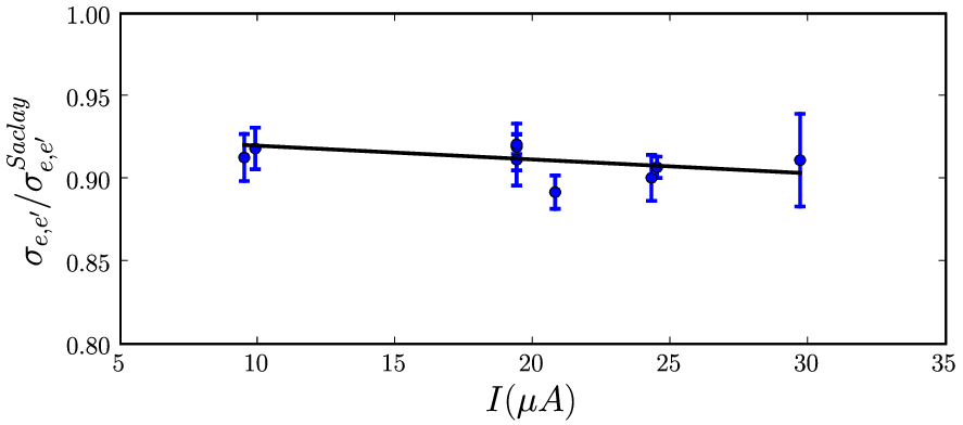
The normalization factor varied between 1.082 at 5 A and 1.12 at 40 A. Contributions to this factor are the change of the effective target thickness due to the horizontal rastering of the beam position (4 %), the 3 % hydrogen admixture to the deuterium gas, and losses of recoil deuterons due to nuclear reactions, estimated to be less than 3 %.
The systematic error of the measured cross sections has been determined to be about 6.2 %. It contains contributions from the uncertainty in the elastic deuteron cross section (2 %), estimated deuteron losses (2.5 %) and the uncertainty of the normalization factor due to the statistical error in the D(e,e′D) cross section (1.7 %).
The error due to the uncertainties in the kinematic variables such as beam energy, beam direction, electron momentum and direction and proton direction was estimated for each bin. Their values lie between 0.3 % and 4 % depending on the kinematics. The largest errors are found for the setting where the protons are almost parallel (central setting where ) to the momentum transfer and the (e,e′p) cross section is dominated by and . For this setting the experimental cross sections were dominated by statistical errors and the extracted provides just an upper limit. For the next setting () they are of the order of 1 % and below for the rest of the data. We have added these errors in quadrature to the statistical ones.
III Determination of
In order to extract the cross sections, the data have been binned in two dimensions, missing energy and missing momentum. The spectra have subsequently been radiatively unfolded and corrected for the coincidence phase space acceptance. For each bin in missing momentum, we obtained the cross section by integrating over missing energy, where the D(e,e′p)n reaction produces a peak at 2.25 MeV.

| kinematics | ||||
|---|---|---|---|---|
| rlt00 | -60 | 60 | 1 | 10 |
| rlt020 | -35 | 35 | 5 | 15 |
| rlt040 | -15 | 15 | 15 | 25 |
| rlt048 | -15 | 15 | 20 | 30 |
| rlt1800 | 120 | 240 | 1 | 10 |
| rlt18020 | 145 | 215 | 5 | 15 |
| rlt18040 | 165 | 195 | 15 | 25 |
| rlt18048 | 165 | 195 | 20 | 30 |
The large acceptances of the spectrometers lead to large regions in the kinematic variables that have been sampled at each spectrometer setting. Cuts in (the angle between the ejected proton and the momentum transfer), and have been applied (figure 4 and table 2) in order to have well defined the kinematical regions sampled in each spectrometer setting. In spite of these cuts different missing energy and missing momentum bins average the cross section over smaller, different kinematic areas.
In order to take this into account we used a Monte-Carlo calculation, including the full theoretical model, to determine the average of the relevant kinematical variables for each missing energy/missing momentum bin. The average variables evaluated this way were the electron scattering angle (), the momentum and energy transfers () and the final proton momentum . From these averaged quantities and the missing momentum we subsequently calculated the average angle between the outgoing proton and the momentum transfer . This quantity could also have been obtained directly from the Monte-Carlo calculation; however, the D(e,e′p)n kinematics would then have been over-determined and the averaging process would lead to inconsistent kinematic results. We therefore selected to calculate the average value of from the averaged values for , and . The average kinematic variables as a function of missing momentum are shown in figure 5.

From the same calculation we also obtained the averaged values for the Mott cross section, the recoil factor, the kinematical factors for the response functions (i.e. the density matrix for the virtual photon polarization , in eq. (3)) and averages of and . can also be calculated from the averaged kinematical values associated with each data bin.
From the general D(e,e′p)n cross section in (3) one sees that the interference response functions can be extracted from the dependence of the cross section. Most of the data taken in this experiment are in or close to the electron scattering plane, with angles distributed around and . We have decided to extract from the cross section difference:
| (7) |
| (8) |
Here and are averages for the settings centered around and respectively, contains all normalization factors and is the averaged Mott cross section for the bin considered. This separation required that all kinematical variables except are identical. This is in general not the case as can be seen from figure 5. Only the central bin approximately satisfies this condition.
In addition to the small overlap between the two settings, the cross section determined for each missing momentum bin differs slightly from the cross section corresponding to the averaged kinematics associated with this bin. This difference will also introduce a systematic error in the extracted response function and needs to be corrected.
To correct for these effects we have calculated the averaged cross section for each missing momentum bin. For one set of calculations we used PWIA and the momentum distribution calculated with the Paris potential, for the other set of calculations we interpolated the theoretical response functions that include FSI, MEC and IC. These two calculations allow one also to estimate the model dependence for correction factors derived for the effects above.
The ratio between the cross section calculated for the averaged kinematics () and the averaged cross section () for each bin can be used to correct the experimental cross section for bin centering ()
| (9) |
Bin centering corrections (9) are typically of the order of a few percent and are larger at the edge of the acceptance compared to its center (figure 6). The largest shifts occur for the data set. The ratios calculated using PWIA are considerably smaller and are also shown in figure 6.

The bin-centered, ’experimental’ cross sections (9) have now well defined kinematic variables that can be used for comparison with theory without the need to perform a Monte-Carlo averaging of the theoretical cross sections. The drawback of bin center corrections is that one introduces a certain amount of model-dependence. Comparing the bin-centering corrections between the full calculation and PWIA gives an estimate of the model dependence of this approach (figure 6,7).
When we used the theoretical cross sections for the extraction of to test the extraction method we found deviations of up to 15 % between the obtained value for and the theoretical one. This was due to the mis-match in the kinematical variables between the and the kinematic settings for each corresponding missing momentum bin. These differences affect especially the photon density matrix and the Mott cross section which should be independent of .
The same model used to determine the bin centering correction has therefore been applied in a second step to correct for these kinematical differences for each bin as follows: we calculated the cross sections for exactly the same kinematics as the data with changed to the appropriate values of the data leading to . The experimental cross sections for the data sets have then been corrected for the kinematic mis-match by multiplying them bin-wise by .
| (10) |
The matched cross sections have then been used to determine and the asymmetry defined as
| (11) |
The experimental results for using the procedure described above are shown in figure 9 and the one for are shown in figure 10.
To estimate the effect of the model dependence of the entire procedure on the extraction of we have performed the same analysis using PWIA in order to calculate the theoretical cross sections. The ratio between obtained using the full calculation which includes FSI, MEC, IC and RC and obtained using PWIA is shown in figure 7. In general the observed deviations are considerably smaller than the error of and except for the edges of the acceptance smaller than 10 %. For the comparisons with the calculations we always used those experimental values that have been extracted using the full calculation for the correction factors.

IV Results and Discussion
A comparison of the calculated cross sections to the experimental ones as a function of missing momentum is presented in figure 8. The red circles correspond to kinematic settings centered around and the blue triangles correspond to kinematic settings centered around . In order to better compare the experimental cross sections to the calculated ones the ratio between experiment and calculation is shown in the lower two graphs in figure 8.

While the general behavior of the cross sections as a function of missing momentum is well reproduced by the calculation, one finds that the experimental cross sections are generally of the order of 10 to 20 % below the calculation especially for the kinematics. This behavior is similar to what has been observed in other experiments as well and needs further study [2, 4, 5].
The coupled channel calculation, including explicit pionic degrees of freedom and using the Bonn-OBEPR potential seems to agree best with the experimental data (solid lines). This is the same calculation that was compared to experimental results in a determination of the interference response function in the delta region by Pellegrino et al. [9]. Among the impulse approximation based calculations the best agreement is obtained by the calculation including FSI and RC (N+R), while the one including all contributions (N+MEC+IC+R), systematically over-predicts the cross sections for as well as for .

In figure 10 the extracted asymmetry (11) is compared to the one determined from the coupled channel model (CC, solid curve). The calculation systematically deviates from the experiment in the same region where the cross sections deviate. This indicates that this discrepancy is not due to an overall normalization factor in the cross sections since an overall factor would cancel in . The observed deviation could be due to a discrepancy in the interference response function or the longitudinal () and/or the transverse () responses. We compared the extracted response function to the one calculated from the coupled channel calculation (figure 9) and found that the calculation agrees well with the experiment within the experimental error bars. This suggests that the observed differences in the cross section is not due to a difference in but due to a discrepancy in the longitudinal/transverse responses.
This is in agreement with the experiments mentioned in the introduction that extracted and and found that the experimental value of is systematically smaller than the calculated [13, 15].

V Summary and Conclusion
In summary, we have measured the D(e,e′p)n cross section for missing momenta up to 290 MeV/c at and and extracted the interference response function . This response is well reproduced by the coupled channel calculation using the Bonn potential. The measured cross sections are systematically below the calculations by 10 - 20 % for missing momenta between 100 MeV/c and 200 MeV/c. This same behavior can also be observed in other experiments [2, 4, 5]. The fact that the extracted experimental values for agree well with the calculation leads to the conclusion that the cross section deviations at lower missing momenta are due to differences in the longitudinal and/or the transverse responses. To further investigate this issue would require an L/T separation which has not been carried out for this kinematics to date.
Acknowledgements.
Numerical results in electronic form are available from the first author. This work was supported in part by the Department of Energy, DOE grant DE–FG02–99ER41065 and by the Deutsche Forschungsgemeinschaft (SFB 201)Appendix A Kinematics Tables and Numerical Results
Tables 3 – 10 contain the average kinematic setting for each bin in missing momentum together with the experimental cross section, the bin corrected cross section and the statistical and systematic errors. Tables 11 – 14 contain the extracted response function including statistical and systematic errors, the asymmetry including all its errors and the corrected experimental cross section for the setting matched to the kinematics at as described in the text above.
| (MeV) | ||||||||||
|---|---|---|---|---|---|---|---|---|---|---|
| 35.0 | 45.17 | 190.0 | 609.5 | 3.07 | 32.91 | 621.3 | 3.49e-06 | 3.44e-06 | 3.5e-07 | 2.4e-07 |
| 45.0 | 45.15 | 193.3 | 609.0 | 3.85 | 32.46 | 626.4 | 1.90e-06 | 1.83e-06 | 1.6e-07 | 1.3e-07 |
| 55.0 | 45.07 | 196.3 | 607.9 | 4.62 | 33.55 | 630.9 | 1.22e-06 | 1.15e-06 | 1.2e-07 | 7.9e-08 |
| 65.0 | 44.99 | 200.0 | 606.7 | 5.34 | 38.75 | 636.3 | 6.89e-07 | 6.19e-07 | 8.4e-08 | 4.4e-08 |
| 75.0 | 44.88 | 201.7 | 605.3 | 6.23 | 45.38 | 637.9 | 5.88e-07 | 5.18e-07 | 1.6e-07 | 3.7e-08 |
| (MeV) | ||||||||||
|---|---|---|---|---|---|---|---|---|---|---|
| 85.0 | 44.92 | 199.4 | 605.8 | 7.48 | 8.35 | 632.3 | 3.67e-07 | 3.55e-07 | 4.6e-09 | 2.3e-08 |
| 95.0 | 44.91 | 202.6 | 605.5 | 8.30 | 8.39 | 636.3 | 1.73e-07 | 1.65e-07 | 3.3e-09 | 1.1e-08 |
| 105.0 | 44.90 | 204.8 | 605.3 | 9.20 | 8.27 | 638.3 | 1.17e-07 | 1.11e-07 | 2.7e-09 | 7.3e-09 |
| 115.0 | 44.89 | 204.7 | 605.2 | 10.25 | 8.27 | 636.0 | 7.51e-08 | 7.11e-08 | 1.4e-09 | 4.7e-09 |
| 125.0 | 44.89 | 204.5 | 605.2 | 11.29 | 8.19 | 633.4 | 4.91e-08 | 4.66e-08 | 1.1e-09 | 3.1e-09 |
| 135.0 | 44.89 | 204.2 | 605.3 | 12.33 | 8.15 | 630.3 | 3.46e-08 | 3.27e-08 | 8.9e-10 | 2.2e-09 |
| 145.0 | 44.86 | 200.4 | 605.2 | 13.50 | 8.27 | 621.1 | 2.36e-08 | 2.21e-08 | 6.6e-10 | 1.5e-09 |
| (MeV) | ||||||||||
|---|---|---|---|---|---|---|---|---|---|---|
| 180.0 | 44.89 | 204.9 | 605.1 | 16.88 | 7.52 | 618.2 | 6.48e-09 | 6.30e-09 | 5.4e-10 | 4.0e-10 |
| 190.0 | 44.89 | 201.1 | 605.5 | 18.02 | 7.52 | 607.7 | 5.40e-09 | 5.12e-09 | 4.2e-10 | 3.4e-10 |
| 200.0 | 44.90 | 200.4 | 605.6 | 19.05 | 7.52 | 602.6 | 4.11e-09 | 3.85e-09 | 3.6e-10 | 2.6e-10 |
| 210.0 | 44.90 | 201.2 | 605.6 | 20.05 | 7.39 | 600.1 | 3.29e-09 | 3.08e-09 | 3.3e-10 | 2.0e-10 |
| 220.0 | 44.90 | 201.1 | 605.6 | 21.08 | 7.25 | 595.9 | 2.68e-09 | 2.52e-09 | 2.8e-10 | 1.7e-10 |
| 230.0 | 44.90 | 200.8 | 605.6 | 22.12 | 7.11 | 590.8 | 2.31e-09 | 2.19e-09 | 2.8e-10 | 1.4e-10 |
| 240.0 | 44.90 | 197.9 | 605.8 | 23.21 | 7.16 | 581.1 | 2.60e-09 | 2.52e-09 | 3.0e-10 | 1.6e-10 |
| 250.0 | 44.92 | 192.5 | 606.4 | 24.31 | 7.16 | 566.3 | 3.69e-09 | 3.69e-09 | 5.4e-10 | 2.3e-10 |
| (MeV) | ||||||||||
|---|---|---|---|---|---|---|---|---|---|---|
| 230.0 | 45.00 | 202.3 | 606.5 | 22.06 | 6.83 | 593.8 | 2.56e-09 | 2.48e-09 | 2.5e-10 | 1.6e-10 |
| 240.0 | 45.02 | 200.5 | 607.0 | 23.13 | 6.88 | 585.8 | 2.22e-09 | 2.16e-09 | 2.4e-10 | 1.4e-10 |
| 250.0 | 45.03 | 200.4 | 607.1 | 24.17 | 6.69 | 580.8 | 2.25e-09 | 2.20e-09 | 2.1e-10 | 1.4e-10 |
| 260.0 | 45.03 | 200.3 | 607.1 | 25.22 | 6.43 | 575.6 | 2.24e-09 | 2.21e-09 | 2.3e-10 | 1.4e-10 |
| 270.0 | 45.03 | 200.6 | 607.1 | 26.27 | 6.17 | 571.1 | 1.93e-09 | 1.92e-09 | 2.2e-10 | 1.2e-10 |
| 280.0 | 45.05 | 200.5 | 607.2 | 27.33 | 5.96 | 565.7 | 1.94e-09 | 1.94e-09 | 2.6e-10 | 1.2e-10 |
| 290.0 | 45.10 | 196.1 | 608.1 | 28.43 | 5.96 | 551.8 | 2.82e-09 | 2.86e-09 | 3.6e-10 | 1.8e-10 |
| (MeV) | ||||||||||
|---|---|---|---|---|---|---|---|---|---|---|
| 35.0 | 45.20 | 191.7 | 609.7 | 2.95 | 145.04 | 624.5 | 3.38e-06 | 3.33e-06 | 2.5e-07 | 2.2e-07 |
| 45.0 | 45.15 | 197.7 | 608.5 | 3.39 | 144.54 | 634.4 | 1.75e-06 | 1.66e-06 | 1.6e-07 | 1.1e-07 |
| 55.0 | 45.13 | 203.7 | 607.7 | 3.77 | 144.67 | 644.2 | 1.34e-06 | 1.25e-06 | 1.3e-07 | 8.7e-08 |
| 65.0 | 45.09 | 209.6 | 606.9 | 4.12 | 145.17 | 653.5 | 8.89e-07 | 8.25e-07 | 9.5e-08 | 5.8e-08 |
| 75.0 | 44.99 | 214.0 | 605.5 | 4.69 | 145.29 | 659.8 | 5.88e-07 | 5.38e-07 | 8.0e-08 | 3.8e-08 |
| 85.0 | 44.94 | 216.4 | 604.8 | 5.64 | 144.87 | 662.6 | 3.86e-07 | 3.55e-07 | 8.5e-08 | 2.5e-08 |
| (MeV) | ||||||||||
|---|---|---|---|---|---|---|---|---|---|---|
| 85.0 | 44.88 | 191.9 | 606.0 | 7.86 | 171.53 | 619.0 | 4.60e-07 | 4.63e-07 | 1.3e-08 | 2.9e-08 |
| 95.0 | 44.89 | 194.9 | 605.8 | 8.73 | 171.61 | 622.5 | 2.96e-07 | 2.96e-07 | 7.7e-09 | 1.9e-08 |
| 105.0 | 44.90 | 197.9 | 605.7 | 9.60 | 171.65 | 626.0 | 2.02e-07 | 2.00e-07 | 5.3e-09 | 1.3e-08 |
| 115.0 | 44.90 | 200.5 | 605.6 | 10.48 | 171.69 | 628.6 | 1.38e-07 | 1.37e-07 | 4.5e-09 | 8.7e-09 |
| 125.0 | 44.90 | 203.2 | 605.4 | 11.36 | 171.69 | 631.0 | 9.09e-08 | 8.96e-08 | 2.7e-09 | 5.7e-09 |
| 125.0 | 44.90 | 203.2 | 605.4 | 11.36 | 171.69 | 631.0 | 9.09e-08 | 9.22e-08 | 2.7e-09 | 5.7e-09 |
| 125.0 | 44.90 | 203.2 | 605.4 | 11.36 | 171.69 | 631.0 | 9.35e-08 | 8.96e-08 | 3.7e-09 | 5.9e-09 |
| 125.0 | 44.90 | 203.2 | 605.4 | 11.36 | 171.69 | 631.0 | 9.35e-08 | 9.22e-08 | 3.7e-09 | 5.9e-09 |
| 135.0 | 44.91 | 206.4 | 605.3 | 12.21 | 171.65 | 634.4 | 7.16e-08 | 7.05e-08 | 2.4e-09 | 4.5e-09 |
| 145.0 | 44.92 | 211.1 | 605.0 | 12.97 | 171.65 | 640.3 | 4.75e-08 | 4.72e-08 | 2.0e-09 | 3.0e-09 |
| 145.0 | 44.92 | 211.1 | 605.0 | 12.97 | 171.65 | 640.3 | 4.75e-08 | 4.81e-08 | 2.0e-09 | 3.0e-09 |
| 145.0 | 44.92 | 211.1 | 605.0 | 12.97 | 171.65 | 640.3 | 4.84e-08 | 4.72e-08 | 2.3e-09 | 3.0e-09 |
| 145.0 | 44.92 | 211.1 | 605.0 | 12.97 | 171.65 | 640.3 | 4.84e-08 | 4.81e-08 | 2.3e-09 | 3.0e-09 |
| 155.0 | 44.92 | 215.2 | 604.7 | 13.77 | 171.69 | 644.9 | 3.71e-08 | 3.72e-08 | 2.0e-09 | 2.3e-09 |
| (MeV) | ||||||||||
|---|---|---|---|---|---|---|---|---|---|---|
| 180.0 | 44.87 | 191.0 | 606.0 | 17.22 | 172.10 | 592.9 | 1.75e-08 | 1.77e-08 | 1.1e-09 | 1.1e-09 |
| 190.0 | 44.89 | 194.5 | 605.9 | 18.17 | 172.14 | 595.6 | 1.34e-08 | 1.34e-08 | 8.4e-10 | 8.3e-10 |
| 200.0 | 44.89 | 197.7 | 605.7 | 19.12 | 172.10 | 597.8 | 1.02e-08 | 1.01e-08 | 6.4e-10 | 6.4e-10 |
| 200.0 | 44.89 | 197.7 | 605.7 | 19.12 | 172.10 | 597.8 | 1.02e-08 | 9.23e-09 | 6.4e-10 | 6.4e-10 |
| 200.0 | 44.89 | 197.7 | 605.7 | 19.12 | 172.10 | 597.8 | 9.33e-09 | 1.01e-08 | 6.1e-10 | 5.8e-10 |
| 200.0 | 44.89 | 197.7 | 605.7 | 19.12 | 172.10 | 597.8 | 9.33e-09 | 9.23e-09 | 6.1e-10 | 5.8e-10 |
| 210.0 | 44.90 | 200.9 | 605.5 | 20.06 | 172.14 | 599.6 | 8.43e-09 | 8.25e-09 | 5.6e-10 | 5.2e-10 |
| 220.0 | 44.90 | 202.8 | 605.4 | 21.04 | 172.14 | 599.1 | 6.10e-09 | 5.93e-09 | 4.5e-10 | 3.8e-10 |
| 230.0 | 44.91 | 203.6 | 605.5 | 22.05 | 172.14 | 596.2 | 4.44e-09 | 4.29e-09 | 3.6e-10 | 2.8e-10 |
| 240.0 | 44.93 | 206.8 | 605.5 | 23.00 | 172.14 | 597.7 | 4.15e-09 | 4.06e-09 | 3.7e-10 | 2.6e-10 |
| 250.0 | 44.94 | 212.1 | 605.2 | 23.88 | 172.14 | 603.2 | 3.70e-09 | 3.71e-09 | 4.2e-10 | 2.3e-10 |
| 260.0 | 44.97 | 219.4 | 605.1 | 24.65 | 172.31 | 612.3 | 3.59e-09 | 3.63e-09 | 6.3e-10 | 2.2e-10 |
| (MeV) | ||||||||||
|---|---|---|---|---|---|---|---|---|---|---|
| 230.0 | 45.00 | 194.3 | 607.2 | 22.20 | 172.39 | 578.8 | 5.13e-09 | 5.10e-09 | 3.8e-10 | 3.2e-10 |
| 240.0 | 45.00 | 198.1 | 606.9 | 23.18 | 172.39 | 581.4 | 4.28e-09 | 4.21e-09 | 3.1e-10 | 2.7e-10 |
| 250.0 | 45.01 | 201.1 | 606.7 | 24.16 | 172.39 | 582.2 | 3.46e-09 | 3.37e-09 | 2.5e-10 | 2.2e-10 |
| 260.0 | 45.02 | 202.1 | 606.8 | 25.19 | 172.39 | 579.2 | 3.33e-09 | 3.23e-09 | 2.3e-10 | 2.1e-10 |
| 270.0 | 45.03 | 202.5 | 606.9 | 26.24 | 172.44 | 574.6 | 2.31e-09 | 2.23e-09 | 2.0e-10 | 1.4e-10 |
| 280.0 | 45.06 | 204.5 | 607.0 | 27.25 | 172.48 | 573.3 | 1.87e-09 | 1.82e-09 | 1.8e-10 | 1.2e-10 |
| 290.0 | 45.09 | 208.8 | 607.0 | 28.22 | 172.48 | 576.2 | 2.01e-09 | 1.99e-09 | 2.3e-10 | 1.3e-10 |
| 300.0 | 45.10 | 214.1 | 606.8 | 29.16 | 172.44 | 580.8 | 1.95e-09 | 1.96e-09 | 2.1e-10 | 1.2e-10 |
| 35.0 | 1.20e-08 | 5.4e-08 | 4.4e-08 | 1.40e-02 | 6.2e-02 | 5.1e-02 | 3.34e-06 |
| 45.1 | 1.92e-08 | 2.8e-08 | 2.2e-08 | 4.23e-02 | 6.2e-02 | 4.8e-02 | 1.68e-06 |
| 55.0 | -1.69e-08 | 2.1e-08 | 1.5e-08 | -5.27e-02 | 6.6e-02 | 4.7e-02 | 1.27e-06 |
| 65.0 | -3.14e-08 | 1.6e-08 | 9.6e-09 | -1.54e-01 | 7.9e-02 | 4.5e-02 | 8.43e-07 |
| 85.0 | -1.12e-08 | 1.6e-09 | 4.1e-09 | -1.22e-01 | 1.5e-02 | 4.4e-02 | 4.54e-07 |
| 95.1 | -1.47e-08 | 9.5e-10 | 2.4e-09 | -2.79e-01 | 1.5e-02 | 4.1e-02 | 2.92e-07 |
| 105.1 | -1.03e-08 | 6.8e-10 | 1.7e-09 | -2.85e-01 | 1.6e-02 | 4.1e-02 | 1.99e-07 |
| 115.1 | -7.68e-09 | 5.4e-10 | 1.1e-09 | -3.15e-01 | 1.7e-02 | 4.0e-02 | 1.36e-07 |
| 125.1 | -5.09e-09 | 3.3e-10 | 7.5e-10 | -3.16e-01 | 1.6e-02 | 4.0e-02 | 8.97e-08 |
| 125.1 | -5.09e-09 | 3.3e-10 | 7.5e-10 | -3.16e-01 | 1.6e-02 | 4.0e-02 | 9.22e-08 |
| 125.1 | -5.39e-09 | 4.5e-10 | 7.7e-10 | -3.29e-01 | 2.0e-02 | 4.0e-02 | 8.97e-08 |
| 125.1 | -5.39e-09 | 4.5e-10 | 7.7e-10 | -3.29e-01 | 2.0e-02 | 4.0e-02 | 9.22e-08 |
| 135.1 | -4.49e-09 | 3.0e-10 | 5.8e-10 | -3.67e-01 | 1.8e-02 | 3.8e-02 | 7.06e-08 |
| 145.1 | -2.96e-09 | 2.5e-10 | 3.8e-10 | -3.66e-01 | 2.2e-02 | 3.8e-02 | 4.76e-08 |
| 145.1 | -2.96e-09 | 2.5e-10 | 3.8e-10 | -3.66e-01 | 2.2e-02 | 3.8e-02 | 4.85e-08 |
| 145.1 | -3.07e-09 | 2.7e-10 | 3.9e-10 | -3.74e-01 | 2.4e-02 | 3.8e-02 | 4.76e-08 |
| 145.1 | -3.07e-09 | 2.7e-10 | 3.9e-10 | -3.74e-01 | 2.4e-02 | 3.8e-02 | 4.85e-08 |
| 180.0 | -1.29e-09 | 1.4e-10 | 1.4e-10 | -4.57e-01 | 4.1e-02 | 3.5e-02 | 1.69e-08 |
| 190.0 | -9.57e-10 | 1.1e-10 | 1.1e-10 | -4.37e-01 | 4.0e-02 | 3.6e-02 | 1.31e-08 |
| 200.0 | -7.47e-10 | 8.7e-11 | 8.1e-11 | -4.45e-01 | 4.3e-02 | 3.5e-02 | 1.00e-08 |
| 200.0 | -7.47e-10 | 8.7e-11 | 8.1e-11 | -4.45e-01 | 4.3e-02 | 3.5e-02 | 9.15e-09 |
| 200.0 | -6.39e-10 | 8.3e-11 | 7.5e-11 | -4.07e-01 | 4.6e-02 | 3.7e-02 | 1.00e-08 |
| 200.0 | -6.39e-10 | 8.3e-11 | 7.5e-11 | -4.07e-01 | 4.6e-02 | 3.7e-02 | 9.15e-09 |
| 210.1 | -6.31e-10 | 7.7e-11 | 6.7e-11 | -4.56e-01 | 4.8e-02 | 3.5e-02 | 8.25e-09 |
| 220.1 | -4.22e-10 | 6.3e-11 | 5.0e-11 | -4.04e-01 | 5.3e-02 | 3.7e-02 | 5.95e-09 |
| 230.1 | -2.65e-10 | 5.5e-11 | 3.7e-11 | -3.28e-01 | 6.5e-02 | 3.9e-02 | 4.33e-09 |
| 240.1 | -2.05e-10 | 5.9e-11 | 3.7e-11 | -2.48e-01 | 6.9e-02 | 4.1e-02 | 4.19e-09 |
| 230.0 | -3.02e-10 | 5.5e-11 | 4.3e-11 | -3.26e-01 | 5.5e-02 | 3.9e-02 | 4.88e-09 |
| 240.0 | -2.51e-10 | 4.8e-11 | 3.7e-11 | -3.16e-01 | 5.9e-02 | 4.0e-02 | 4.15e-09 |
| 250.0 | -1.50e-10 | 4.1e-11 | 3.2e-11 | -2.12e-01 | 5.7e-02 | 4.2e-02 | 3.38e-09 |
| 260.0 | -1.34e-10 | 4.1e-11 | 3.1e-11 | -1.91e-01 | 6.0e-02 | 4.2e-02 | 3.25e-09 |
| 270.1 | -4.37e-11 | 3.8e-11 | 2.4e-11 | -8.03e-02 | 7.0e-02 | 4.4e-02 | 2.26e-09 |
| 280.0 | 9.76e-12 | 4.2e-11 | 2.2e-11 | 1.95e-02 | 8.3e-02 | 4.4e-02 | 1.87e-09 |
| 290.0 | 9.07e-11 | 5.7e-11 | 2.9e-11 | 1.39e-01 | 8.3e-02 | 4.3e-02 | 2.17e-09 |
References
- [1] T. de Forest, Nucl. Phys. A 392, 232 (1983).
- [2] M. Bernheim et al., Nucl. Phys. A 365, 349 (1981).
- [3] S. Turck-Chieze et al., Phys. Lett. B 142, 145 (1984).
- [4] K.I. Blomqvist et al., Phys. Lett. B 429, 33 (1998a).
- [5] P.E Ulmer et al., Phys. Rev. Lett. 89, 062301 (2002).
- [6] H. Arenhövel, Nucl. Phys. A 384, 287 (1982).
- [7] H. Arenhövel, W. Leidemann, and L. Tomusiak, Eur. Phys. J. A 23, 147 (2005).
- [8] Z.-L. Zhou et al., Phys. Rev. Lett. 87, 172301 (2001).
- [9] A. Pellegrino et al., Phys. Rev. Lett. 78, 4011 (1997).
- [10] Z.-L. Zhou et al., Proccedings of the MIT-Bates Workshop (1998).
- [11] M. van der Schaar et al., Phys. Rev. Lett. 66, 2855 (1991).
- [12] M. van der Schaar et al., Phys. Rev. Lett. 68, 776 (1992).
- [13] D. Jordan et al., Phys. Rev. Lett. 76, 1579 (1996).
- [14] W.-J. Kasdorp et al., Phys. Lett. B 393, 42 (1997).
- [15] J. E. Ducret et al., Phys. Rev. C 49, 1783 (1994).
- [16] H. J. Bulten et al., Phys. Rev. Lett. 74, 4775 (1995).
- [17] K.I. Blomqvist et al., Nucl. Instr. and Meth. A 403, 263 (1998b).
- [18] S. Platchkov et al., Nucl. Phys. A 510, 740 (1990).
- [19] S. Auffret et al., Phys. Rev. Lett. 54, 649 (1985).