DISTINCT DISTANCES IN GRAPH DRAWINGS

Paz Carmi¹¹ 1 School of Computer Science, Carleton University, Ottawa, Canada ({paz,vida,morin}@scs.carleton.ca). Research supported by NSERC. Vida Dujmović¹¹ 1 School of Computer Science, Carleton University, Ottawa, Canada ({paz,vida,morin}@scs.carleton.ca). Research supported by NSERC. Pat Morin¹¹ 1 School of Computer Science, Carleton University, Ottawa, Canada ({paz,vida,morin}@scs.carleton.ca). Research supported by NSERC. David R. Wood²² 2 Departament de Matemàtica Aplicada II, Universitat Politècnica de Catalunya, Barcelona, Spain (david.wood@upc.es). Research supported by a Marie Curie Fellowship from the European Commission under contract MEIF-CT-2006-023865, and by the projects MEC MTM2006-01267 and DURSI 2005SGR00692.

August 24, 2026

Abstract

The distance-number of a graph $G$ is the minimum number of distinct edge-lengths over all straight-line drawings of $G$ in the plane. This definition generalises many well-known concepts in combinatorial geometry. We consider the distance-number of trees, graphs with no $K^{-}_{4}$ -minor, complete bipartite graphs, complete graphs, and cartesian products. Our main results concern the distance-number of graphs with bounded degree. We prove that $n$ -vertex graphs with bounded maximum degree and bounded treewidth have distance-number in $\mathcal{O}(\log n)$ . To conclude such a logarithmic upper bound, both the degree and the treewidth need to be bounded. In particular, we construct graphs with treewidth $2$ and polynomial distance-number. Similarly, we prove that there exist graphs with maximum degree $5$ and arbitrarily large distance-number. Moreover, as $\Delta$ increases the existential lower bound on the distance-number of $\Delta$ -regular graphs tends to $\Omega(n^{0.864138})$ .

1 Introduction

This paper initiates the study of the minimum number of distinct edge-lengths in a drawing of a given graph¹¹ 1 We consider graphs that are simple, finite, and undirected. The vertex set of a graph $G$ is denoted by $V(G)$ , and its edge set by $E(G)$ . A graph with $n$ vertices, $m$ edges and maximum degree at most $\Delta$ is an $n$ -vertex, $m$ -edge, degree- $\Delta$ graph. A graph in which every vertex has degree $\Delta$ is $\Delta$ -regular. For $S\subseteq V(G)$ , let $G[S]$ be the subgraph of $G$ induced by $S$ , and let $G-S:=G[V(G)\setminus S]$ . For each vertex $v\in V(G)$ , let $G-v:=G-\{v\}$ . Standard notation is used for graphs: complete graphs $K_{n}$ , complete bipartite graphs $K_{m,n}$ , paths $P_{n}$ , and cycles $C_{n}$ . A graph $H$ is a minor of a graph $G$ if $H$ can be obtained from a subgraph of $G$ by contracting edges. Throughout the paper, $c$ is a positive constant. Of course, different occurrences of $c$ might denote different constants.. A degenerate drawing of a graph $G$ is a function that maps the vertices of $G$ to distinct points in the plane, and maps each edge $vw$ of $G$ to the open straight-line segment joining the two points representing $v$ and $w$ . A drawing of $G$ is a degenerate drawing of $G$ in which the image of every edge of $G$ is disjoint from the image of every vertex of $G$ . That is, no vertex intersects the interior of an edge. In what follows, we often make no distinction between a vertex or edge in a graph and its image in a drawing.

The distance-number of a graph $G$ , denoted by $\textup{{dn}}(G)$ , is the minimum number of distinct edge-lengths in a drawing of $G$ . The degenerate distance-number of $G$ , denoted by $\textup{{ddn}}(G)$ , is the minimum number of distinct edge-lengths in a degenerate drawing of $G$ . Clearly, $\textup{{ddn}}(G)\leq\textup{{dn}}(G)$ for every graph $G$ . Furthermore, if $H$ is a subgraph of $G$ then $\textup{{ddn}}(H)\leq\textup{{ddn}}(G)$ and $\textup{{dn}}(H)\leq\textup{{dn}}(G)$ .

1.1 Background and Motivation

The degenerate distance-number and distance-number of a graph generalise various concepts in combinatorial geometry, which motivates their study.

A famous problem raised by Erdős [15] asks for the minimum number of distinct distances determined by $n$ points in the plane²² 2 For a detailed exposition on distinct distances in point sets refer to Chapters $10$ – $13$ of the monograph by Pach and Agarwal [37].. This problem is equivalent to determining the degenerate distance-number of the complete graph $K_{n}$ . We have the following bounds on $\textup{{ddn}}(K_{n})$ , where the lower bound is due to Katz and Tardos [25] (building on recent advances by Solymosi and Tóth [47], Solymosi et al. [46], and Tardos [50]), and the upper bound is due to Erdős [15].

Lemma 1 ([25, 15]).

The degenerate distance-number of $K_{n}$ satisfies

\Omega(n^{0.864137})\leq\textup{{ddn}}(K_{n})\leq\frac{cn}{\sqrt{\log n}}\kern 5.0pt.

Observe that no three points are collinear in a (non-degenerate) drawing of $K_{n}$ . Thus $\textup{{dn}}(K_{n})$ equals the minimum number of distinct distances determined by $n$ points in the plane with no three points collinear. This problem was considered by Szemerédi (see Theorem 13.7 in [37]), who proved that every such point set contains a point from which there are at least $\left\lceil\frac{n-1}{3}\right\rceil$ distinct distances to the other points. Thus we have the next result, where the upper bound follows from the drawing of $K_{n}$ whose vertices are the points of a regular $n$ -gon, as illustrated in Figure 1(a).

Refer to caption — Figure 1: (a) A drawing of $K_{10}$ with five edge-lengths, and (b) a drawing of $K_{5,5}$ with three edge-lengths.

Lemma 2 (Szemerédi).

The distance-number of $K_{n}$ satisfies

\left\lceil\frac{n-1}{3}\right\rceil\leq\textup{{dn}}(K_{n})\leq\left\lfloor\frac{n}{2}\right\rfloor\kern 5.0pt.

Note that Lemmas 1 and 2 show that for every sufficiently large complete graph, the degenerate distance-number is strictly less than the distance-number. Indeed, $\textup{{ddn}}(K_{n})\in o(\textup{{dn}}(K_{n}))$ .

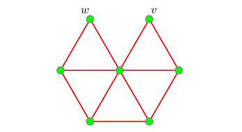
Degenerate distance-number generalises another concept in combinatorial geometry. The unit-distance graph of a set $S$ of points in the plane has vertex set $S$ , where two vertices are adjacent if and only if they are at unit-distance; see [45, 36, 35, 39, 42, 23] for example. The famous Hadwiger-Nelson problem asks for the maximum chromatic number of a unit-distance graph. Every unit-distance graph $G$ has $\textup{{ddn}}(G)=1$ . But the converse is not true, since a degenerate drawing allows non-adjacent vertices to be at unit-distance. Figure 2 gives an example of a graph $G$ with $\textup{{dn}}(G)=\textup{{ddn}}(G)=1$ that is not a unit-distance graph. In general, $\textup{{ddn}}(G)=1$ if and only if $G$ is isomorphic to a subgraph of a unit-distance graph.

The maximum number of edges in a unit-distance graph is an old open problem. The best construction, due to Erdős [15], gives an $n$ -vertex unit-distance graph with $n^{1+c/\log\log n}$ edges. The best upper bound on the number of edges is $cn^{4/3}$ , due to Spencer et al. [48]. (Székely [49] found a simple proof for this upper bound based on the crossing lemma.)

More generally, many recent results in the combinatorial geometry literature provide upper bounds on the number of times the $d$ most frequent inter-point distances can occur between a set of $n$ points. Such results are equivalent to upper bounds on the number of edges in an $n$ -vertex graph with degenerate distance number $d$ . This suggests the following extremal function. Let $\textup{$\textsf{ex}$}(n,d)$ be the maximum number of edges in an $n$ -vertex graph $G$ with $\textup{{ddn}}(G)\leq d$ .

Since every graph $G$ is the union of $\textup{{ddn}}(G)$ subgraphs of unit-distance graphs, the above result by Spencer et al. [48] implies:

Lemma 3 (Spencer et al. [48]).

\textup{$\textsf{ex}$}(n,d)\leq cdn^{4/3}.

Equivalently, the distance-numbers of every $n$ -vertex $m$ -edge graph $G$ satisfy

\textup{{dn}}(G)\geq\textup{{ddn}}(G)\geq cmn^{-4/3}\kern 5.0pt.

Results by Katz and Tardos [25] (building on recent advances by Solymosi and Tóth [47], Solymosi et al. [46], and Tardos [50]) imply:

Lemma 4 (Katz and Tardos [25]).

\textup{$\textsf{ex}$}(n,d)\in\mathcal{O}\big(n^{1.457341}d^{0.627977}\big)\kern 5.0pt.

Equivalently, the distance-numbers of every $n$ -vertex $m$ -edge graph $G$ satisfy

\textup{{dn}}(G)\geq\textup{{ddn}}(G)\in\Omega(m^{1.592412}\,n^{-2.320687})\kern 5.0pt.

Note that Lemma 4 improves upon Lemma 3 whenever $\textup{{ddn}}(G)>n^{1/3}$ . Also note that Lemma 4 implies the lower bound in Lemma 2.

1.2 Our Results

The above results give properties of various graphs defined with respect to the inter-point distances of a set of points in the plane. This paper, which is more about graph drawing than combinatorial geometry, reverses this approach, and asks for a drawing of a given graph with few inter-point distances.

Our first results provide some general families of graphs, namely trees and graphs with no $K^{-}_{4}$ -minor, that are unit-distance graphs (Section 2). Here $K^{-}_{4}$ is the graph obtained from $K_{4}$ by deleting one edge. Then we give bounds on the distance-numbers of complete bipartite graphs (Section 3).

Our main results concern graphs of bounded degree (Section 4). We prove that for all $\Delta\geq 5$ there are degree- $\Delta$ graphs with unbounded distance-number. Moreover, for $\Delta\geq 7$ we prove a polynomial lower bound on the distance-number (of some degree- $\Delta$ graph) that tends to $\Omega(n^{0.864138})$ for large $\Delta$ . On the other hand, we prove that graphs with bounded degree and bounded treewidth have distance-number in $\mathcal{O}(\log n)$ . Note that bounded treewidth alone does not imply a logarithmic bound on distance-number since $K_{2,n}$ has treewidth $2$ and degenerate distance-number $\Theta(\sqrt{n})$ (see Section 3).

Then we establish an upper bound on the distance-number in terms of the bandwidth (Section 5). Then we consider the distance-number of the cartesian product of graphs (Section 6). We conclude in Section 7 with a discussion of open problems related to distance-number.

1.3 Higher-Dimensional Relatives

Graph invariants related to distances in higher dimensions have also been studied. Erdős, Harary, and Tutte [16] defined the dimension of a graph $G$ , denoted by $\textup{{dim}}(G)$ , to be the minimum integer $d$ such that $G$ has a degenerate drawing in $\Re^{d}$ with straight-line edges of unit-length. They proved that $\textup{{dim}}(K_{n})=n-1$ , the dimension of the $n$ -cube is $2$ for $n\geq 2$ , the dimension of the Peterson graph is $2$ , and $\textup{{dim}}(G)\leq 2\cdot\chi(G)$ for every graph $G$ . (Here $\chi(G)$ is the chromatic number of $G$ .) The dimension of complete $3$ -partite graphs and wheels were determined by Buckley and Harary [10].

The unit-distance graph of a set $S\subseteq\Re^{d}$ has vertex set $S$ , where two vertices are adjacent if and only if they are at unit-distance. Thus $\textup{{dim}}(G)\leq d$ if and only if $G$ is isomorphic to a subgraph of a unit-distance graph in $\Re^{d}$ . Maehara [32] proved for all $d$ there is a finite bipartite graph (which thus has dimension at most $4$ ) that is not a unit-distance graph in $\Re^{d}$ . This highlights the distinction between dimension and unit-distance graphs. Maehara [32] also proved that every finite graph with maximum degree $\Delta$ is a unit-distance graph in $\Re^{\Delta(\Delta^{2}-1)/2}$ , which was improved to $\Re^{2\Delta}$ by Maehara and Rödl [33]. These results are in contrast to our result that graphs of bounded degree have arbitrarily large distance-number.

A graph is $d$ -realizable if, for every mapping of its vertices to (not-necessarily distinct) points in $\Re^{p}$ with $p\geq d$ , there exists such a mapping in $\Re^{d}$ that preserves edge-lengths. For example, $K_{3}$ is $2$ -realizable but not $1$ -realizable. Belk and Connelly [6] and Belk [5] proved that a graph is $2$ -realizable if and only if it has treewidth at most $2$ . They also characterized the $3$ -realizable graphs as those with no $K_{5}$ -minor and no $K_{2,2,2}$ -minor.

2 Some Unit-Distance Graphs

This section shows that certain families of graphs are unit-distance graphs. The proofs are based on the fact that two distinct circles intersect in at most two points. We start with a general lemma. A graph $G$ is obtained by pasting subgraphs $G_{1}$ and $G_{2}$ on a cut-vertex $v$ of $G$ if $G=G_{1}\cup G_{2}$ and $V(G_{1})\cap V(G_{2})=\{v\}$ .

Lemma 5.

Let $G$ be the graph obtained by pasting subgraphs $G_{1}$ and $G_{2}$ on a vertex $v$ . Then:
(a) if $\textup{{ddn}}(G_{1})=\textup{{ddn}}(G_{2})=1$ then $\textup{{ddn}}(G)=1$ , and
(b) if $\textup{{dn}}(G_{1})=\textup{{dn}}(G_{2})=1$ then $\textup{{dn}}(G)=1$ .

Proof.

We prove part (b). Part (a) is easier. Let $D_{i}$ be a drawing of $G_{i}$ with unit-length edges. Translate $D_{2}$ so that $v$ appears in the same position in $D_{1}$ and $D_{2}$ . A rotation of $D_{2}$ about $v$ is bad if its union with $D_{1}$ is not a drawing of $G$ . That is, some vertex in $D_{2}$ coincides with the closure of some edge of $D_{1}$ , or vice versa. Since $G$ is finite, there are only finitely many bad rotations. Since there are infinitely many rotations, there exists a rotation that is not bad. That is, there exists a drawing of $G$ with unit-length edges. ∎

We have a similar result for unit-distance graphs.

Lemma 6.

Let $G_{1}$ and $G_{2}$ be unit-distance graphs. Let $G$ be the (abstract) graph obtained by pasting $G_{1}$ and $G_{2}$ on a vertex $v$ . Then $G$ is isomorphic to a unit-distance graph.

Proof.

The proof is similar to the proof of Lemma 5, except that we must ensure that the distance between vertices in $G_{1}-v$ and vertices in $G_{2}-v$ (which are not adjacent) is not $1$ . Again this will happen for only finitely many rotations. Thus there exists a rotation that works. ∎

Since every tree can be obtained by pasting a smaller tree with $K_{2}$ , Lemma 6 implies that every tree is a unit-distance graph. The following is a stronger result.

Lemma 7.

Every tree $T$ has a crossing-free³³ 3 A drawing is crossing-free if no pair of edges intersect. drawing in the plane such that two vertices are adjacent if and only if they are unit-distance apart.

Proof.

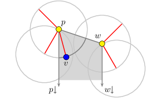
For a point $v=(\textup{{x}}(v),\textup{{y}}(v))$ in the plane, let $v\!\!\downarrow$ be the ray from $v$ to $(\textup{{x}}(v),-\infty)$ . We proceed by induction on $n$ with the following hypothesis: Every tree $T$ with $n$ vertices has the desired drawing, such that the vertices have distinct x-coordinates, and for each vertex $u$ , the ray $u\!\!\downarrow$ does not intersect $T$ . The statement is trivially true for $n\leq 2$ . For $n>2$ , let $v$ be a leaf of $T$ with parent $p$ . By induction, $T-v$ has the desired drawing. Let $w$ be a vertex of $T-v$ , such that no vertex has its x-coordinate between $\textup{{x}}(p)$ and $\textup{{x}}(w)$ . Thus the drawing of $T-v$ does not intersect the open region $R$ of the plane bounded by the two rays $p\!\!\downarrow$ and $w\!\!\downarrow$ , and the segment $pw$ . Let $A$ be the intersection of $R$ with the unit-circle centred at $p$ . Thus $A$ is a circular arc. Place $v$ on $A$ , so that the distance from $v$ to every vertex except $p$ is not $1$ . This is possible since $A$ is infinite, and there are only finitely many excluded positions on $A$ (since $A$ intersects a unit-circle centred at a vertex except $p$ in at most two points). Since there are no elements of $T-v$ in $R$ , there are no crossings in the resulting drawing and the induction invariants are maintained for all vertices of $T$ . ∎

Recall that $K^{-}_{4}$ is the graph obtained from $K_{4}$ by deleting one edge.

Theorem 1.

Every $K^{-}_{4}$ -minor-free graph $G$ has a drawing such that vertices are adjacent if and only if they are unit-distance apart. In particular, $G$ is isomorphic to a unit-distance graph and $\textup{{ddn}}(G)=\textup{{dn}}(G)=1$ .

Proof.

Clearly we can assume that $G$ is connected. If $G$ is not $2$ -connected then $G$ can be obtained by pasting smaller graphs with no $K^{-}_{4}$ -minor on a single vertex. Thus by Lemma 6, it suffices to prove that every $2$ -connected $K^{-}_{4}$ -minor-free graph is a unit-distance graph. Below we prove that every $2$ -connected graph $G$ with no $K^{-}_{4}$ -minor is a cycle. The result follows since $C_{n}$ is a unit-distance graph (draw a regular $n$ -gon).

Suppose on the contrary that $G$ has a vertex $v$ of degree at least $3$ . Let $x,y,z$ be the neighbours of $v$ . So there is an $xy$ -path $P$ avoiding $v$ (since $G$ is $2$ -connected) and avoiding $z$ (since $G$ is $K^{-}_{4}$ -minor free). Similarly, there is an $xz$ -path $Q$ avoiding $v$ . If $x$ is the only vertex in both $P$ and $Q$ , then the cycle $(x,P,y,v,z,Q)$ plus the edge $xv$ is a subdivision of $K^{-}_{4}$ . Now assume that $P$ and $Q$ intersect at some other vertex. Let $t$ be the first vertex on $P$ starting at $x$ that is also in $Q$ . Then the cycle $(x,Q,z,v)$ plus the sub-path of $P$ between $x$ and $t$ is a subdivision of $K^{-}_{4}$ . Hence $G$ has no vertex of degree at least $3$ . Therefore $G$ is a cycle, as desired. ∎

3 Complete Bipartite Graphs

This section considers the distance-numbers of complete bipartite graphs $K_{m,n}$ . Since $K_{1,n}$ is a tree, $\textup{{ddn}}(K_{1,n})=\textup{{dn}}(K_{1,n})=1$ by Lemma 7. The next case, $K_{2,n}$ , is also easily handled.

Lemma 8.

The distance-numbers of $K_{2,n}$ satisfy

\textup{{ddn}}(K_{2,n})=\textup{{dn}}(K_{2,n})=\left\lceil\sqrt{\frac{n}{2}}\right\rceil\kern 5.0pt.

Proof.

Let $G=K_{2,n}$ with colour classes $A=\{v,w\}$ and $B$ , where $|B|=n$ . We first prove the lower bound. Consider a degenerate drawing of $G$ with $\textup{{ddn}}(G)$ edge-lengths. The vertices in $B$ lie on the intersection of $\textup{{ddn}}(G)$ concentric circles centered at $v$ and $\textup{{ddn}}(G)$ concentric circles centered at $w$ . Since two distinct circles intersect in at most two points, $n\leq 2\,\textup{{ddn}}(G)^{2}$ . Thus $\textup{{ddn}}(K_{2,n})\geq\left\lceil\sqrt{\frac{n}{2}}\right\rceil$

For the upper bound, position $v$ at $(-1,0)$ and $w$ at $(1,0)$ . As illustrated in Figure 4, draw $\left\lceil\sqrt{\frac{n}{2}}\right\rceil$ circles centered at each of $v$ and $w$ with radii ranging strictly between $1$ and $2$ , such that the intersections of the circles together with $v$ and $w$ define a set of points with no three points collinear. (This can be achieved by choosing the radii iteratively, since for each circle $C$ , there are finitely many forbidden values for the radius of $C$ .) Each pair of non-concentric circles intersect in two points. Thus the number of intersection points is at least $n$ . Placing the vertices of $B$ at these intersection points results in a drawing of $K_{2,n}$ with $\left\lceil\sqrt{\frac{n}{2}}\right\rceil$ edge-lengths.∎

Now we determine $\textup{{ddn}}(K_{3,n})$ to within a constant factor.

Lemma 9.

The degenerate distance-number of $K_{3,n}$ satisfies

\left\lceil\sqrt{\frac{n}{2}}\right\rceil\leq\textup{{ddn}}(K_{3,n})\leq 3\left\lceil\sqrt{\frac{n}{2}}\right\rceil-1\kern 5.0pt.

Proof.

The lower bound follows from Lemma 8 since $K_{2,n}$ is a subgraph of $K_{3,n}$ .

Now we prove the upper bound. Let $A$ and $B$ be the colour classes of $K_{3,n}$ , where $|A|=3$ and $|B|=n$ . Place the vertices in $A$ at $(-1,0)$ , $(0,0)$ , and $(1,0)$ . Let $d:=\left\lceil\sqrt{\frac{n}{2}}\right\rceil$ . For $i\in[d]$ , let

r_{i}:=\sqrt{1+\frac{i}{d+1}}\kern 5.0pt.

Note that $1<r_{i}<2$ . Let $R_{i}$ be the circle centred at $(-1,0)$ with radius $r_{i}$ . For $j\in[d]$ , let $S_{j}$ be the circle centred at $(1,0)$ with radius $r_{j}$ . Observe that each pair of circles $R_{i}$ and $S_{j}$ intersect in exactly two points. Place the vertices in $B$ at the intersection points of these circles. This is possible since $2d^{2}\geq n$ .

Let $(x,y)$ and $(x,-y)$ be the two points where $R_{i}$ and $S_{j}$ intersect. Thus $(x+1)^{2}+y^{2}=r_{i}^{2}$ and $(x-1)^{2}+y^{2}=r_{j}^{2}$ . It follows that

x^{2}+y^{2}=\frac{i}{d+1}+2x=\frac{j}{d+1}-2x\kern 5.0pt.

Thus $2(x^{2}+y^{2})=\frac{i+j}{d+1}$ . That is, the distance from $(x,y)$ to $(0,0)$ equals

\sqrt{\frac{i+j}{2d+2}},

which is the same distance from $(x,-y)$ to $(0,0)$ . Thus the distance from each vertex in $B$ to $(0,0)$ is one of $2d-1$ values (determined by $i+j$ ). The distance from each vertex in $B$ to $(-1,0)$ and to $(1,0)$ is one of $d$ values. Hence the degenerate distance-number of $K_{3,n}$ is at most $3d-1=3\left\lceil\sqrt{\frac{n}{2}}\right\rceil-1$ . ∎

Now consider the distance-number of a general complete bipartite graph.

Lemma 10.

For all $n\geq m$ , the distance-numbers of $K_{m,n}$ satisfy

\Omega\Big(\frac{mn}{(m+n)^{1.457341}}\Big)^{1/0.627977}\leq\textup{{ddn}}(K_{m,n})\leq\textup{{dn}}(K_{m,n})\leq\left\lceil\frac{n}{2}\right\rceil\kern 5.0pt.

In particular,

\Omega(n^{0.864137})\leq\textup{{ddn}}(K_{n,n})\leq\textup{{dn}}(K_{n,n})\leq\left\lceil\frac{n}{2}\right\rceil\kern 5.0pt.

Proof.

The lower bounds follow from Lemma 4. For the upper bound on $\textup{{dn}}(K_{n,n})$ , position the vertices on a regular $2n$ -gon $(v_{1},v_{2},\dots,v_{2n})$ alternating between the colour classes, as illustrated in Figure 1(b). In the resulting drawing of $K_{n,n}$ , the number of edge-lengths is $|\{(i+j)\mod n\,:\,v_{i}v_{j}\in E(K_{n,n})\}|$ . Since $v_{i}v_{j}$ is an edge if and only if $i+j$ is odd, the number of edge-lengths is $\left\lceil\frac{n}{2}\right\rceil$ . The upper bound on $\textup{{dn}}(K_{n,m})$ follows since $K_{n,m}$ is a subgraph of $K_{n,n}$ . ∎

4 Bounded degree graphs

Lemma 8 implies that if a graph has two vertices with many common neighbours then its distance-number is necessarily large. Thus it is natural to ask whether graphs of bounded degree have bounded distance-number. This section provides a negative answer to this question.

4.1 Bounded degree graphs with $\Delta\geq 7$

This section proves that for all $\Delta\geq 7$ there are $\Delta$ -regular graphs with unbounded distance-number. Moreover, the lower bound on the distance-number is polynomial in the number of vertices. The basic idea of the proof is to show that there are more $\Delta$ -regular graphs than graphs with bounded distance-number.

It will be convenient to count labelled graphs. Let $\mathcal{G}\langle{n,\Delta}\rangle$ denote the family of labelled $\Delta$ -regular $n$ -vertex graphs. Let $\mathcal{G}\langle{n,m,d}\rangle$ denote the family of labelled $n$ -vertex $m$ -edge graphs with degenerate distance-number at most $d$ . Our results follow by comparing a lower bound on $|\mathcal{G}\langle{n,\Delta}\rangle|$ with an upper bound on $|\mathcal{G}\langle{n,m,d}\rangle|$ with $m=\frac{\Delta n}{2}$ , which is the number of edges in a $\Delta$ -regular $n$ -vertex graph.

The lower bound in question is known. In particular, the first asymptotic bounds on the number of labelled $\Delta$ -regular $n$ -vertex graphs were independently determined by Bender and Canfield [7] and Wormald [52]. McKay [34] further refined these results. We will use the following simple lower bound derived by Barát et al. [4] from the result of McKay [34].

Lemma 11 ([4, 7, 52, 34]).

For all integers $\Delta\geq 1$ and $n\geq c\Delta$ , the number of labelled $\Delta$ -regular $n$ -vertex graphs satisfies

|\mathcal{G}\langle{n,\Delta}\rangle|\geq\Big(\frac{n}{3\Delta}\Big)^{\Delta n/2}.

The proof of our upper bound on $|\mathcal{G}\langle{n,m,d}\rangle|$ uses the following special case of the Milnor-Thom theorem by Rónyai et al. [43]. Let $\mathcal{P}=(P_{1},P_{2},\dots,P_{t})$ be a sequence of polynomials on $p$ variables over $\Re$ . The zero-pattern of ${\mathcal{P}}$ at $u\in\Re^{p}$ is the set $\{i:1\leq i\leq t,\,P_{i}(u)=0\}$ .

Lemma 12 ([43]).

Let ${\mathcal{P}}=(P_{1},P_{2},\dots,P_{t})$ be a sequence of polynomials of degree at most $\delta\geq 1$ on $p\leq t$ variables over $\Re$ . Then the number of zero-patterns of ${\mathcal{P}}$ is at most $\binom{\delta t}{p}$ .

Recall that $\textup{$\textsf{ex}$}(n,d)$ is the maximum number of edges in an $n$ -vertex graph $G$ with $\textup{{ddn}}(G)\leq d$ . Bounds on this function are given in Lemmas 3 and 4. Our upper bound on $|\mathcal{G}\langle{n,m,d}\rangle|$ is expressed in terms of $\textup{$\textsf{ex}$}(n,d)$ .

Lemma 13.

The number of labelled $n$ -vertex $m$ -edge graphs with $\textup{{ddn}}(G)\leq d$ satisfies

|\mathcal{G}\langle{n,m,d}\rangle|\leq\left(\frac{\textup{{e}}nd}{2}\right)^{2n+d}\binom{\textup{$\textsf{ex}$}(n,d)}{m}\kern 5.0pt,

where e is the base of the natural logarithm.

Proof.

Let $V(G)=\{1,2,\dots,n\}$ for every $G\in\mathcal{G}\langle{n,m,d}\rangle$ . For every $G\in\mathcal{G}\langle{n,m,d}\rangle$ , there is a point set

S(G)=\{(x_{i}(G),y_{i}(G))\,:\,1\leq i\leq n\}

and a set of edge-lengths

L(G)=\{\ell_{k}(G)\,:\,1\leq k\leq d\},

such that $G$ has a degenerate drawing in which each vertex $i$ is represented by the point $(x_{i}(G),y_{i}(G))$ and the length of each edge in $E(G)$ is in $L(G)$ . Fix one such degenerate drawing of $G$ .

For all $i,j,k$ with $1\leq i<j\leq n$ and $1\leq k\leq d$ , and for every graph $G\in\mathcal{G}\langle{n,m,d}\rangle$ , define

P_{i,j,k}(G):=(x_{j}(G)-x_{i}(G))^{2}+(y_{j}(G)-y_{i}(G))^{2}-\ell_{k}(G)^{2}\kern 5.0pt.

Consider ${\mathcal{P}}:=\{P_{i,j,k}:1\leq i<j\leq n,1\leq k\leq d\}$ to be a set of $\binom{n}{2}d$ degree- $2$ polynomials on the set of $2n+d$ variables $\{x_{1},x_{2},\dots,x_{n},y_{1},y_{2},\dots,y_{n},\ell_{1},\ell_{2},\dots,\ell_{d}\}$ . Observe that

$P_{i,j,k}(G)=0$ if and only if the distance between vertices $i$ and $j$ in the

degenerate drawing of $G$ is $\ell_{k}(G)$ .

$(\star)$

Recall the well-known fact that $\binom{a}{b}\leq(\frac{\textup{{e}}a}{b})^{b}$ . By Lemma 12 with $t=\binom{n}{2}d$ , $\delta=2$ and $p=2n+d$ , the number of zero-patterns determined by ${\mathcal{P}}$ is at most

\binom{2\binom{n}{2}d}{2n+d}\leq\left(\frac{2\textup{{e}}\binom{n}{2}d}{2n+d}\right)^{2n+d}<\left(\frac{\textup{{e}}n^{2}d}{2n+d}\right)^{2n+d}<\left(\frac{\textup{{e}}n^{2}d}{2n}\right)^{2n+d}=\left(\frac{\textup{{e}}nd}{2}\right)^{2n+d}\kern 5.0pt.

Fix a zero-pattern $\sigma$ of $\mathcal{P}$ . Let $\mathcal{G}_{\sigma}$ be the set of graphs $G$ in $\mathcal{G}\langle{n,m,d}\rangle$ such that $\sigma$ is the zero-pattern of ${\mathcal{P}}$ evaluated at $G$ . To bound $|\mathcal{G}\langle{n,m,d}\rangle|$ we now bound $|{\mathcal{G}}_{\sigma}|$ . Let $H_{\sigma}$ be the graph with vertex set $V(H_{\sigma})=\{1,\dots,n\}$ and edge set $E(H_{\sigma})$ where $ij\in E(H_{\sigma})$ if and only if $ij\in E(G)$ for some $G\in\mathcal{G}_{\sigma}$ . Consider a degenerate drawing of an arbitrary graph $G\in\mathcal{G}_{\sigma}$ on the point set $S(G)$ . By $(\star)$ , $S(G)$ and $L(G)$ define a degenerate drawing of $H$ with $d$ edge-lengths. Thus $\textup{{ddn}}(H_{\sigma})\leq d$ and by assumption, $|E(H_{\sigma})|\leq\textup{$\textsf{ex}$}(n,d)$ . Since every graph in $\mathcal{G}_{\sigma}$ is a subgraph of $H_{\sigma}$ , $|\mathcal{G}_{\sigma}|\leq\binom{|E(H_{\sigma})|}{m}$ . Therefore,

|\mathcal{G}\langle{n,m,d}\rangle|\leq\left(\frac{\textup{{e}}nd}{2}\right)^{2n+d}\binom{|E(H_{\sigma})|}{m}\leq\left(\frac{\textup{{e}}nd}{2}\right)^{2n+d}\binom{\textup{$\textsf{ex}$}(n,d)}{m},

as required. ∎

By comparing the lower bound in Lemma 11 and the upper bound in Lemma 13 we obtain the following result.

Lemma 14.

Suppose that for some real numbers $\alpha$ and $\beta$ with $\beta>0$ and $1<\alpha<2<\alpha+\beta$ ,

\textup{$\textsf{ex}$}(n,d)\in\mathcal{O}(n^{\alpha}d^{\beta})\kern 5.0pt.

Then for every integer $\Delta>\frac{4}{2-\alpha}$ , for all $\varepsilon>0$ , and for all sufficiently large $n>n(\alpha,\beta,\Delta,\varepsilon)$ , there exists a $\Delta$ -regular $n$ -vertex graph $G$ with degenerate distance-number

\textup{{ddn}}(G)>n^{\frac{2-\alpha}{\beta}-\frac{(2-\alpha+\beta)(4+2\varepsilon)}{\beta^{2}\Delta+4\beta}}\kern 5.0pt.

Proof.

In this proof, $\alpha$ , $\beta$ , $\Delta$ and $\epsilon$ are fixed numbers satisfying the assumptions of the lemma. Let $d$ be the maximum degenerate distance number of a graph in $\mathcal{G}\langle{n,\Delta}\rangle$ . The result will follow by showing that for all sufficiently large $n>n(\alpha,\beta,\Delta,\varepsilon)$ ,

d>n^{\frac{2-\alpha}{\beta}-\frac{(2-\alpha+\beta)(4+2\varepsilon)}{\beta^{2}\Delta+4\beta}}\kern 5.0pt.

By the definition of $d$ , and since every $\Delta$ -regular $n$ -vertex graph has $\frac{\Delta n}{2}$ edges, every graph in $\mathcal{G}\langle{n,\Delta}\rangle$ is also in $\mathcal{G}\langle{n,\frac{\Delta n}{2},d}\rangle$ . By Lemma 11 with $n\geq c\Delta$ , and by Lemma 13,

\displaystyle\Big(\frac{n}{3\Delta}\Big)^{\Delta n/2}\leq|\mathcal{G}\langle{n,\Delta}\rangle|\leq|\mathcal{G}\langle{n,\frac{\Delta n}{2},d}\rangle|\leq\left(\frac{\textup{{e}}nd}{2}\right)^{2n+d}\binom{\textup{$\textsf{ex}$}(n,d)}{\Delta n/2}\kern 5.0pt.

Since $\textup{$\textsf{ex}$}(n,d)\in\mathcal{O}(n^{\alpha}d^{\beta})$ , and since $d$ is a function of $n$ , there is a constant $c$ such that $\textup{$\textsf{ex}$}(n,d)\leq cn^{\alpha}d^{\beta}$ for sufficiently large $n$ . Thus (and since $\binom{a}{b}\leq(\frac{\textup{{e}}a}{b})^{b}$ ),

\displaystyle\Big(\frac{n}{3\Delta}\Big)^{\Delta n/2}\leq\left(\frac{\textup{{e}}nd}{2}\right)^{2n+d}\binom{cn^{\alpha}d^{\beta}}{\Delta n/2}\leq\left(\frac{\textup{{e}}nd}{2}\right)^{2n+d}\left(\frac{2\textup{{e}}cn^{\alpha}d^{\beta}}{\Delta n}\right)^{\Delta n/2}\kern 5.0pt.

Hence

\displaystyle n^{\Delta n}\leq 3^{\Delta n}\left(\frac{\textup{{e}}nd}{2}\right)^{4n+2d}\left(2\textup{{e}}cn^{\alpha-1}d^{\beta}\right)^{\Delta n}\kern 5.0pt.

By Lemma 2, $d\leq\textup{{ddn}}(K_{n})\leq\frac{cn}{\sqrt{\log n}}$ , implying $2d\leq\varepsilon n$ for all large $n>n(\varepsilon)$ . Thus

\displaystyle n^{\Delta}

\displaystyle\leq 3^{\Delta}\left(\frac{\textup{{e}}nd}{2}\right)^{4+\varepsilon}\left(2\textup{{e}}cn^{\alpha-1}d^{\beta}\right)^{\Delta}\kern 5.0pt.

Hence

\displaystyle n^{(2-\alpha)\Delta-4-\varepsilon}

\displaystyle\leq 3^{\Delta}\left(\frac{\textup{{e}}}{2}\right)^{4+\varepsilon}\left(2\textup{{e}}c\right)^{\Delta}d^{\beta\Delta+4+\varepsilon}\kern 5.0pt.

Observe that $3^{\Delta}\left(\frac{\textup{{e}}}{2}\right)^{4+\varepsilon}(2\textup{{e}}c)^{\Delta}\leq n^{\varepsilon}$ for all large $n>n(\Delta,\varepsilon)$ . Thus

\displaystyle n^{(2-\alpha)\Delta-4-2\varepsilon}

\displaystyle\leq d^{\beta\Delta+4+\varepsilon}

Hence

\displaystyle d\geq n^{\frac{(2-\alpha)\Delta-4-2\varepsilon}{\beta\Delta+4+\varepsilon}}=n^{\frac{2-\alpha}{\beta}-\frac{(2-\alpha+\beta)(4+\varepsilon)+\beta\epsilon}{\beta(\beta\Delta+4+\varepsilon)}}>n^{\frac{2-\alpha}{\beta}-\frac{(2-\alpha+\beta)(4+2\varepsilon)}{\beta^{2}\Delta+4\beta}}\kern 5.0pt,

as required. ∎

We can now state the main results of this section. By Lemma 3, the conditions of Lemma 14 are satisfied with $\alpha=\frac{4}{3}$ and $\beta=1$ ; thus together they imply:

Theorem 2.

For every integer $\Delta\geq 7$ , for all $\varepsilon>0$ , and for all sufficiently large $n>n(\Delta,\varepsilon)$ , there exists a $\Delta$ -regular $n$ -vertex graph $G$ with degenerate distance-number

\textup{{ddn}}(G)>n^{\frac{2}{3}-\frac{20+10\varepsilon}{3\Delta+12}}\kern 5.0pt.

By Lemma 4, the conditions of Lemma 14 are satisfied with $\alpha=1.457341$ and $\beta=0.627977$ ; thus together they imply:

Theorem 3.

For every integer $\Delta\geq 8$ , for all $\varepsilon>0$ , and for all sufficiently large $n>n(\Delta,\varepsilon)$ , there exists a $\Delta$ -regular $n$ -vertex graph $G$ with degenerate distance-number

\textup{{ddn}}(G)>n^{0.864138-\frac{4.682544+2.341272\varepsilon}{0.394355\Delta+2.511908}}\kern 5.0pt.

Note that the bound given in Theorem 3 is better than the bound in Theorem 2 for $\Delta\geq 17$ .

4.2 Bounded degree graphs with $\Delta\geq 5$

Theorem 2 shows that for $\Delta\geq 7$ and for sufficiently large $n$ , there is an $n$ -vertex degree- $\Delta$ graph whose degenerate distance-number is at least polynomial in $n$ . We now prove that the degenerate distance-number of degree- $5$ graphs can also be arbitrarily large. However, the lower bound we obtain in this case is polylogarithmic in $n$ . The proof is inspired by an analogous proof about the slope-number of degree- $5$ graphs, due to Pach and Pálvölgyi [38].

Theorem 4.

For all $d\in{\mathbb{N}}$ , there is a degree- $5$ graph $G$ with degenerate distance-number $\textup{{ddn}}(G)>d$ .

Proof.

Consider the following degree- $5$ graph $G$ . For $n\equiv 0\pmod{6}$ , let $F$ be the graph with vertex set $\{v_{1},v_{2},\dots,v_{n}\}$ and edge set $\{v_{i}v_{j}\,:\,|i-j|\leq 2\}$ . Let $S:=\{v_{i}\,:\,i\equiv 1\pmod{3}\}$ . No pair of vertices in $S$ are adjacent in $F$ , and $|S|=\frac{n}{3}$ is even.

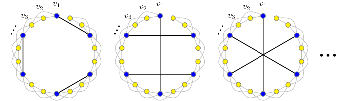
Let $\mathcal{M}$ denote the set of all perfect matchings on $S$ . For each perfect matching $M_{k}\in\mathcal{M}$ , let $G_{k}:=F\cup M_{k}$ . As illustrated in Figure 6, let $G$ be the disjoint union of all the $G_{k}$ . Thus the number of connected components of $G$ is $|\mathcal{M}|$ , which is at least $(\frac{n}{9})^{n/6}$ by Lemma 11 with $\Delta=1$ . Here we consider perfect matchings to be $1$ -regular graphs. (It is remarkable that even with $\Delta=1$ , Lemma 11 gives such an accurate bound, since the actual number of matchings in $S$ is $\sqrt{2}(\frac{n}{3\textup{{e}}})^{n/6}$ ignoring lower order additive terms⁴⁴ 4 For even $n$ , let $f(n)$ be the number of perfect matchings of $[n]$ . Here we determine the asymptotics of $f$ . In every such matching, $n$ is matched with some number in $[n-1]$ , and the remaining matching is isomorphic to a perfect matching of $[n-2]$ . Every matching obtained in this way is distinct. Thus $f(n)=(n-1)\cdot f(n-2)$ , where $f(2)=1$ . Hence $f(n)=(n-1)!!=(n-1)(n-3)(n-5)\dots 1$ , where $!!$ is the double factorial function. Now $(2n-1)!!=\frac{(2n)!}{2^{n}n!}$ . Thus $f(n)=\frac{n!}{2^{n/2}(n/2)!}\approx\sqrt{2}\,(\frac{n}{\textup{{e}}})^{n/2}$ by Stirling’s Approximation..)

Suppose, for the sake of contradiction, that for some constant $d$ , for all $n\in{\mathbb{N}}$ such that $n\equiv 0\pmod{6}$ , $G$ has a degenerate drawing $D$ with at most $d$ edge-lengths.

Label the edges of $G$ that are in the copies of $F$ by their length in $D$ . Let $\ell_{k}(i,j)$ be the label of the edge $v_{i}v_{j}$ in the copy of $F$ in the component $G_{k}$ of $G$ . This defines a labelling of the components of $G$ . Since $F$ has $2n-3$ edges and each edge in $F$ receives one of $d$ labels, there are at most $d^{2n-3}$ distinct labellings of the components of $G$ .

Let $D_{k}$ be the degenerate drawing of $G_{k}$ obtained from $D$ by a translation and rotation so that $v_{1}$ is at $(0,0)$ and $v_{2}$ is at $(\ell_{k}(1,2),0)$ . We say that two components $G_{q}$ and $G_{r}$ of $G$ determine the same set of points if for all $i\in[n]$ , the vertex $v_{i}$ in $D_{q}$ is at the same position as the vertex $v_{i}$ in $D_{r}$ .

Partition the components of $G$ into the minimum number of parts such that all the components in each part have the same labelling and determine the same set of points.

Observe that two components of $G$ with the same labelling do not necessarily determine the same set of points. However, the number of point sets determined by the components with a given labelling can be bounded as follows. For each component $G_{k}$ of $G$ , $v_{1}$ is at $(0,0)$ and $v_{2}$ is at $(\ell_{k}(i,j),0)$ in $D_{k}$ . Thus for a fixed labelling, the positions of $v_{1}$ and $v_{2}$ in $D_{k}$ are determined. Now for $i\geq 3$ , in each component $G_{k}$ , the vertex $v_{i}$ is positioned in $D_{k}$ at the intersection of the circle of radius $\ell_{k}(i-1,i)$ centered at $v_{i-1}$ and the circle of radius $\ell_{k}(i-2,i)$ centered at $v_{i-2}$ . Thus there are at most two possible locations for $v_{i}$ (for a fixed labelling). Hence the components with the same labelling determine at most $2^{n-2}$ distinct points sets. Therefore the number of parts in the partition is at most $d^{2n-3}\cdot 2^{n-2}<(2d^{2})^{n}$ .

Finally, we bound the number of components in each part, $R$ , of the partition. Let $H_{R}$ be the graph with vertex set $V(H_{R})=\{v_{1},\dots,v_{n}\}$ where $v_{i}v_{j}\in E(H_{R})$ if and only if $v_{i}v_{j}\in E(G_{k})$ for some component $G_{k}\in R$ . Since the graphs in $R$ determine the same set of points, the union of the degenerate drawings $D_{k}$ , over all $G_{k}\in R$ , determines a degenerate drawing of $H_{R}$ with $d$ edge-lengths. Thus $\textup{{ddn}}(H_{R})\leq d$ and by Lemma 3, $|E(H_{R})|\leq cdn^{4/3}$ for some constant $c>0$ . Every component in $R$ is a subgraph of $H_{R}$ , and any two components in $R$ differ only by the choice of a matching on $S$ . Each such matching has $\frac{n}{6}$ edges. Thus the number of components of $G$ in $R$ is at most

\binom{|E(H_{R})|}{n/6}\leq\binom{cdn^{4/3}}{n/6}\leq\left(\frac{\textup{{e}}cdn^{4/3}}{n/6}\right)^{n/6}\leq\big(6\textup{{e}}cd\big)^{n/6}n^{n/18}\kern 5.0pt.

Hence $|\mathcal{M}|<(2d^{2})^{n}\cdot(6\textup{{e}}cd)^{n/6}n^{n/18}$ , and by the lower bound on $|\mathcal{M}|$ from the start of the proof,

\left(\frac{n}{9}\right)^{n/6}\leq|\mathcal{M}|<(2d^{2})^{n}\cdot(6\textup{{e}}cd)^{n/6}n^{n/18}\kern 5.0pt.

The desired contradiction follows for all $n\geq(3456\textup{{e}}cd^{13})^{3/2}$ . ∎

4.3 Graphs with bounded degree and bounded treewidth

This section proves a logarithmic upper bound on the distance-number of graphs with bounded degree and bounded treewidth. Treewidth is an important parameter in Robertson and Seymour’s theory of graph minors and in algorithmic complexity (see the surveys [8, 41]). It can be defined as follows. A graph $G$ is a $k$ -tree if either $G=K_{k+1}$ , or $G$ has a vertex $v$ whose neighbourhood is a clique of order $k$ and $G-v$ is a $k$ -tree. For example, every $1$ -tree is a tree and every tree is a $1$ -tree. Then the treewidth of a graph $G$ is the minimum integer $k$ for which $G$ is a subgraph of a $k$ -tree. The pathwidth of $G$ is the minimum $k$ for which $G$ is a subgraph of an interval⁵⁵ 5 A graph $G$ is an interval graph if each vertex $v\in V(G)$ can be assigned an interval $I_{v}\subset\Re$ such that $I_{w}\cap I_{v}\neq\emptyset$ if and only if $vw\in E(V)$ . graph with no clique of order $k+2$ . Note that an interval graph with no $(k+2)$ -clique is a special case of a $k$ -tree, and thus the treewidth of a graph is at most its pathwidth.

Lemma 7 shows that ( $1$ -)trees have bounded distance-number. However, this is not true for $2$ -trees since $K_{2,n}$ has treewidth (and pathwidth) at most $2$ . By Theorem 3, there are $n$ -vertex graphs of bounded degree with distance-number approaching $\Omega(n^{0.864138})$ . On the other hand, no polynomial lower bound holds for graphs of bounded degree and bounded treewidth, as shown in the following theorem.

Theorem 5.

Let $G$ be a graph with $n$ vertices, maximum degree $\Delta$ , and treewidth $k$ . Then the distance-number of $G$ satisfies

\textup{{dn}}(G)\in\mathcal{O}(\Delta^{4}k^{3}\log n)\kern 5.0pt.

To prove Theorem 5 we use the following lemma, the proof of which is readily obtained by inspecting the proof of Lemma 8 in [14]. An $H$ -partition of a graph $G$ is a partition of $V(G)$ into vertex sets $V_{1},\dots,V_{t}$ such that $H$ is the graph with vertex set $V(H):=\{1,\dots,t\}$ where $ij\in E(H)$ if and only if there exists $v\in V_{i}$ and $w\in V_{j}$ such that $v_{i}v_{j}\in E(G)$ . The width of an $H$ -partition is $\max\{|V_{i}|:1\leq i\leq t\}$ .

Lemma 15 ([14]).

Let $H$ be a graph admitting a drawing $D$ with $s$ distinct edge-slopes and $\ell$ distinct edge-lengths. Let $G$ be a graph admitting an $H$ -partition of width $w$ . Then the distance-number of $G$ satisfies

\textup{{dn}}(G)\leq s\ell w(w-1)+\left\lfloor\frac{w}{2}\right\rfloor+\ell\kern 5.0pt.

Sketch of Proof.

The general approach is to start with $D$ and then replace each vertex of $H$ by a sufficiently scaled down and appropriate rotated copy of the drawing of $K_{w}$ on a regular $w$ -gon. The only difficulty is choosing the rotation and the amount by which to scale the $w$ -gons so that we obtain a (non-degenerate) drawing of $G$ . Refer to [14] for the full proof. ∎

Proof of Theorem 5.

Let $w$ be the minimum width of a $T$ -partition of $G$ in which $T$ is a tree. The best known upper bound is $w\leq\frac{5}{2}(k+1)(\frac{7}{2}\,\Delta(G)-1)$ , which was obtained by Wood [51] using a minor improvement to a similar result by an anonymous referee of the paper by Ding and Oporowski [12]. For each vertex $x\in V(T)$ , there are at most $w\Delta$ edges of $G$ incident to vertices mapped to $x$ . Hence we can assume that $T$ is a forest with maximum degree $w\Delta$ , as otherwise there is an edge of $T$ with no edge of $G$ mapped to it, in which case the edge of $T$ can be deleted. Similarly, $T$ has at most $n$ vertices. Scheffler [44] proved that $T$ has pathwidth at most $\log(2n+1)$ ; see [8]. Dujmović et al. [14] proved that every tree $T$ with pathwidth $p\geq 1$ has a drawing with $\max\{\Delta(T)-1,1\}$ slopes and $2p-1$ edge-lengths. Thus $T$ has a drawing with at most $\Delta w-1$ slopes and at most $2\log(2n+1)-1$ edge-lengths. By Lemma 15,

\textup{{dn}}(G)\leq(\Delta w-1)(2\log(2n+1)-1)w(w-1)+\left\lfloor\frac{w}{2}\right\rfloor+2\log(2n+1)-1,

which is in $\mathcal{O}(\Delta w^{3}\log n)\subseteq\mathcal{O}(\Delta^{4}k^{3}\log n)$ . ∎

Corollary 1.

Every $n$ -vertex graph with bounded degree and bounded treewidth has distance-number $\mathcal{O}(\log n)$ .

Since a path has a drawing with one slope and one edge-length, Lemma 15 with $s=\ell=1$ implies that every graph $G$ with a $P$ -partition of width $k$ for some path $P$ has distance-number $\textup{{dn}}(G)\leq k(k-\tfrac{1}{2})+1$ .

5 Bandwidth

This section establishes an upper bound on the distance-number in terms of the bandwidth. Let $G$ be a graph. A vertex ordering of $G$ is a bijection $\sigma:V(G)\rightarrow\{1,2,\dots,|V(G)|\}$ . The width of $\sigma$ is defined to be $\max\{|\sigma(v)-\sigma(w)|:vw\in E(G)\}$ . The bandwidth of $G$ , denoted by $\textsf{bw}(G)$ , is the minimum width of a vertex ordering of $G$ . The cyclic width of $\sigma$ is defined to be $\max\{\min\{|\sigma(v)-\sigma(w)|,n-|\sigma(v)-\sigma(w)|\}:vw\in E(G)\}$ . The cyclic bandwidth of $G$ , denoted by $\textsf{cbw}(G)$ , is the minimum cyclic width of a vertex ordering of $G$ ; see [11, 28, 53, 20, 30]. Clearly $\textup{$\textsf{cbw}(G)$}\leq\textup{$\textsf{bw}(G)$}$ for every graph $G$ .

Lemma 16.

For every graph $G$ ,

\textup{{dn}}(G)\leq\textup{$\textsf{cbw}(G)$}\leq\textup{$\textsf{bw}(G)$}\kern 5.0pt.

Proof.

Given a vertex ordering $\sigma$ of an $n$ -vertex $G$ , position the vertices of $G$ on a regular $n$ -gon in the order $\sigma$ . We obtain a drawing of $G$ in which the length of each edge $vw$ is determined by

\min\{|\sigma(v)-\sigma(w)|,n-|\sigma(v)-\sigma(w)|\}\kern 5.0pt.

Thus the number of edge-lengths equals

|\{\min\{|\sigma(v)-\sigma(w)|,n-|\sigma(v)-\sigma(w)|\}:vw\in E(G)\}|,

which is at most the cyclic width of $\sigma$ . The result follows. ∎

Corollary 2.

The distance-number of every $n$ -vertex degree- $\Delta$ planar graph $G$ satisfies

\textup{{dn}}(G)\leq\frac{15n}{\log_{\Delta}n}\kern 5.0pt.

Proof.

Böttcher et al. [9] proved that $\textup{$\textsf{bw}(G)$}\leq\frac{15n}{\log_{\Delta}n}$ . The result follows from Lemma 16. ∎

6 Cartesian Products

This section discusses the distance-number of cartesian products of graphs. For graphs $G$ and $H$ , the cartesian product $G\square H$ is the graph with vertex set $V(G\square H):=V(G)\times V(H)$ , where $(v,w)$ is adjacent to $(p,q)$ if and only if (1) $v=p$ and $wq$ is an edge of $H$ , or (2) $w=q$ and $vp$ is an edge of $G$ .

Thus $G\square H$ is the grid-like graph with a copy of $G$ in each row and a copy of $H$ in each column. Type (1) edges form copies of $H$ , and type (2) edges form copies of $G$ . For example, $P_{n}\square P_{n}$ is the planar grid, and $C_{n}\square C_{n}$ is the toroidal grid.

The cartesian product is associative and thus multi-dimensional products are well defined. For example, the $d$ -dimensional product $K_{2}\square K_{2}\square\dots\square K_{2}$ is the $d$ -dimensional hypercube $Q_{d}$ . It is well known that $Q_{d}$ is a unit-distance graph. Horvat and Pisanski [24] proved that the cartesian product operation preserves unit-distance graphs. That is, if $G$ and $H$ are unit-distance graphs, then so is $G\square H$ , as illustrated in Figure 7. The following theorem generalises this result.

Theorem 6.

For all graphs $G$ and $H$ , the distance-numbers of $G\square H$ satisfy

	$\displaystyle\max\{\textup{{ddn}}(G),\textup{{ddn}}(H)\}$	$\displaystyle\leq\textup{{ddn}}(G\square H)\leq\textup{{ddn}}(G)+\textup{{ddn}}(H)-1\kern 5.0pt,\text{ and}$
	$\displaystyle\max\{\textup{{dn}}(G),\textup{{dn}}(H)\}$	$\displaystyle\leq\textup{{dn}}(G\square H)\leq\textup{{dn}}(G)+\textup{{dn}}(H)-1\kern 5.0pt.$

Proof.

The lower bounds follow since $G$ and $H$ are subgraphs of $G\square H$ . We prove the upper bound for $\textup{{dn}}(G\square H)$ . The proof for $\textup{{ddn}}(G\square H)$ is simpler.

Fix a drawing of $G$ with $\textup{{dn}}(G)$ edge-lengths. Let $(\textup{{x}}(v),\textup{{y}}(v))$ be the coordinates of each vertex $v$ of $G$ in this drawing. Fix a drawing of $H$ with $\textup{{dn}}(H)$ edge-lengths, scaled so that one edge-length in the drawing of $G$ coincides with one edge-length in the drawing of $H$ . Let $\alpha$ be a real number in $[0,2\pi)$ . Let $(\textup{{x}}_{\alpha}(w),\textup{{y}}_{\alpha}(w))$ be the coordinates of each vertex $w$ of $G$ in this drawing of $H$ rotated by $\alpha$ degrees about the origin.

Position vertex $(v,w)$ in $G\square H$ at $(\textup{{x}}(v)+\textup{{x}}_{\alpha}(w),\textup{{y}}(v)+\textup{{y}}_{\alpha}(w))$ . This mapping preserves edge-lengths. In particular, the length of a type-(1) edge $(v,u)(v,w)$ equals the length of the edge $uw$ in $H$ , and the length of a type-(2) edge $(u,v)(w,v)$ equals the length of the edge $uw$ in $G$ . Thus for each $\alpha$ , the mapping of $G\square H$ has $\textup{{dn}}(G)+\textup{{dn}}(H)-1$ edge-lengths.

It remains to prove that for some $\alpha$ the mapping of $G\square H$ is a drawing. That is, no vertex intersects the closure of an incident edge. An angle $\alpha$ is bad for a particular vertex/edge pair of $G\square H$ if that vertex intersects the closure of that edge in the mapping with rotation $\alpha$ .

Observe that the trajectory of a vertex $(v,w)$ of $G\square H$ (taken over all $\alpha$ ) is a circle centred at $(\textup{{x}}(v),\textup{{y}}(v))$ with radius $\dist_{H}(0,w)$ .

Now for distinct points $p$ and $q$ and a line $\ell$ , there are only two angles $\alpha$ such that the rotation of $p$ around $q$ by an angle of $\alpha$ contains $\ell$ (since the trajectory of $p$ is a circle that only intersects $\ell$ in two places), and there are only two angles $\alpha$ such that the rotation of $\ell$ around $q$ by an angle of $\alpha$ contains $p$ .

It follows that there are finitely many bad values of $\alpha$ for a particular vertex/edge pair of $G\square H$ . Hence there are finitely many bad values of $\alpha$ in total. Hence some value of $\alpha$ is not bad for every vertex/edge pair in $G\square H$ . Hence $D_{\alpha}$ is a valid drawing of $G\square H$ . ∎

Note that Loh and Teh [31] proved a result analogous to Theorem 6 for dimension.

Let $G^{d}$ be the $d$ -fold cartesian product of a graph $G$ . The same construction used in Theorem 6 proves the following:

Theorem 7.

For every graph $G$ and integer $d\geq 1$ , the distance-numbers of $G^{d}$ satisfy

\textup{{ddn}}(G^{d})=\textup{{ddn}}(G)\quad\text{ and }\quad\textup{{dn}}(G^{d})=\textup{{dn}}(G)\kern 5.0pt.

7 Open Problems

We conclude by mentioning some of the many open problems related to distance-number.

•

What is $\textup{{dn}}(K_{n})$ ? We conjecture that $\textup{{dn}}(K_{n})=\left\lfloor\frac{n}{2}\right\rfloor$ . That is, every set of $n$ points in general position determine at least $\left\lfloor\frac{n}{2}\right\rfloor$ distinct distances. Note that Altman [1], Altman [2] proved this conjecture for points in convex position.
•

What is the relationship between distance-number and degenerate distance-number? In particular, is there a function $f$ such that $\textup{{dn}}(G)\leq f(\textup{{ddn}}(G))$ for every graph $G$ ?
•

Theorems 2, 3 and 4 establish a lower bound for the distance-number of bounded degree graphs. But no non-trivial upper bound is known. Do $n$ -vertex graphs with bounded degree have distance-number in $o(n)$ ?
•

Outerplanar graphs have distance-number in $\mathcal{O}(\Delta^{4}\log n)$ by Theorem 5. Do outerplanar graphs (with bounded degree) have bounded (degenerate) distance-number?
•

Non-trivial lower and upper bounds on the distance-numbers are not known for many other interesting graph families including: degree- $3$ graphs, degree- $4$ graphs, $2$ -degenerate graphs with bounded degree, graphs with bounded degree and bounded pathwidth.
•

As described in Section 1.1, determining the maximum number of times the unit-distance can appear among $n$ points in the plane is a famous open problem. We are unaware if the following apparently simpler tasks have been attempted: Determine the maximum number of times the unit-distance can occur among $n$ points in the plane such that no three are collinear. Similarly, determine the maximum number of edges in an $n$ -vertex graph $G$ with $\textup{{dn}}(G)=1$ .
•

Determining the maximum chromatic number of unit-distance graphs in $\Re^{d}$ is a well-known open problem. The best known upper bound of $(3+o(1))^{d}$ is due to Larman and Rogers [29]. Exponential lower bounds are known [40, 17]. Unit-distance graphs in the plane are $7$ -colourable [19], and thus $\chi(G)\leq 7^{\textup{{ddn}}(G)}$ . Can this bound be improved?
•

Degenerate distance-number is not bounded by any function of dimension since $K_{n,n}$ has dimension $4$ and unbounded degenerate distance-number. On the other hand, $\textup{{dim}}(G)\leq 2\cdot\chi(G)\leq 2\cdot 7^{\textup{{ddn}}(G)}$ . Is $\textup{{dim}}(G)$ bounded by a polynomial function of $\textup{{ddn}}(G)$ ?
•

Every planar graph has a crossing-free drawing. A long standing open problem involving edge-lengths, due to Harborth et al. [26, 21, 22], asks whether every planar graph has a crossing-free drawing in which the length of every edge is an integer. Geelen et al. [18] recently answered this question in the affirmative for cubic planar graphs. Archdeacon [3] extended this question to nonplanar graphs and asked what is the minimum $d$ such that a given graph has a crossing-free drawing in $\Re^{d}$ with integer edge-lengths. Note that every $n$ -vertex graph has such a drawing in $\Re^{n-1}$ .
•

The slope number of a graph $G$ , denoted by $\textup{{sn}}(G)$ , is the minimum number of edge-slopes over all drawings of $G$ . Dujmović et al. [13] established results concerning the slope-number of planar graphs. Keszegh et al. [27] proved that degree- $3$ graphs have slope-number at most $5$ . On the other hand, Barát et al. [4] and Pach and Pálvölgyi [38] independently proved that there are $5$ -regular graphs with arbitrarily large slope number. Moreover, for $\Delta\geq 7$ , Dujmović et al. [14] proved that there are $n$ -vertex degree- $\Delta$ graphs whose slope number is at least $n^{1-\frac{\varepsilon}{\Delta+4}}$ . The proofs of these results are similar to the proofs of Theorems 2, 3 and 4. Given that Theorem 5 also depends on slopes, it it tempting to wonder if there is a deeper connection between slope-number and distance-number. For example, is there a function $f$ such that $\textup{{sn}}(G)\leq f(\Delta(G),\textup{{dn}}(G))$ and/or $\textup{{dn}}(G)\leq f(\textup{{sn}}(G))$ for every graph $G$ . Note that some dependence on $\Delta(G)$ is necessary since $\textup{{sn}}(K_{1,n})\rightarrow\infty$ but $\textup{{dn}}(K_{1,n})=1$ .

References

[1] E. Altman. On a problem of P. Erdős. Amer. Math. Monthly, 70:148–157, 1963.
[2] E. Altman. Some theorems on convex polygons. Canad. Math. Bull., 15:329–340, 1972.
[3] Dan Archdeacon. Planar graphs with integer length straight edges, 1995. http://www.emba.uvm.edu/˜archdeac/problems/integer.htm.
[4] János Barát, Jiří Matoušek, and David R. Wood. Bounded-degree graphs have arbitrarily large geometric thickness. Electron. J. Combin., 13(1):R3, 2006.
[5] Maria Belk. Realizability of graphs in three dimensions. Discrete Comput. Geom., 37:139–162, 2007.
[6] Maria Belk and Robert Connelly. Realizability of graphs. Discrete Comput. Geom., 37:125–137, 2007.
[7] Edward A. Bender and E. Rodney Canfield. The asymptotic number of labeled graphs with given degree sequences. J. Combin. Theory Ser. A, 24:296–307, 1978.
[8] Hans L. Bodlaender. A partial $k$ -arboretum of graphs with bounded treewidth. Theoret. Comput. Sci., 209(1-2):1–45, 1998.
[9] Julia Böttcher, Klaas P. Pruessmann, Anusch Taraz, and Andreas Würfl. Bandwidth, treewidth, separators, expansion, and universality. In Proc. Topological and Geometric Graph Theory (TGGT ’08). 2008.
[10] Fred Buckley and Frank Harary. On the Euclidean dimension of a wheel. Graphs Combin., 4(1):23–30, 1988.
[11] Wai Hong Chan, Peter C. B. Lam, and Wai Chee Shiu. Cyclic bandwidth with an edge added. Discrete Appl. Math., 156(1):131–137, 2008.
[12] Guoli Ding and Bogdan Oporowski. Some results on tree decomposition of graphs. J. Graph Theory, 20(4):481–499, 1995.
[13] Vida Dujmović, David Eppstein, Matthew Suderman, and David R. Wood. Drawings of planar graphs with few slopes and segments. Comput. Geom., 38:194–212, 2007a.
[14] Vida Dujmović, Matthew Suderman, and David R. Wood. Graph drawings with few slopes. Comput. Geom., 38:181–193, 2007b.
[15] Paul Erdős. On sets of distances of $n$ points. Amer. Math. Monthly, 53:248–250, 1946.
[16] Paul Erdős, Frank Harary, and William T. Tutte. On the dimension of a graph. Mathematika, 12:118–122, 1965.
[17] Peter Frankl and Richard M. Wilson. Intersection theorems with geometric consequences. Combinatorica, 1(4):357–368, 1981.
[18] Jim Geelen, Anjie Guo, and David McKinnon. Straight line embeddings of cubic planar graphs with integer edge lengths. J. Graph Theory, to appear.
[19] Hugo Hadwiger and Hans Debrunner. Combinatorial geometry in the plane. Holt, New York, 1964.
[20] Frank Harary, Paul C. Kainen, and Adrian Riskin. Every graph of cyclic bandwidth 3 is toroidal. Bull. Inst. Combin. Appl., 27:81–84, 1999.
[21] Heiko Harborth and Arnfried Kemnitz. Integral representations of graphs. In Contemporary methods in graph theory, pp. 359–367. Bibliographisches Inst., Mannheim, 1990.
[22] Heiko Harborth, Arnfried Kemnitz, Meinhard Möller, and Andreas Süssenbach. Ganzzahlige planare Darstellungen der platonischen Körper. Elem. Math., 42(5):118–122, 1987.
[23] Robert Hochberg and Paul O’Donnell. Some $4$ -chromatic unit-distance graphs without small cycles. Geombinatorics, 5(4):137–141, 1996.
[24] Boris Horvat and Tomaž Pisanski. Products of unit distance graphs. In 6th Slovenian International Conference on Graph Theory. Bled, Slovenia, 2007.
[25] Nets Hawk Katz and Gábor Tardos. A new entropy inequality for the Erdős distance problem. In Towards a theory of geometric graphs, vol. 342 of Contemp. Math., pp. 119–126. Amer. Math. Soc., 2004.
[26] Arnfried Kemnitz and Heiko Harborth. Plane integral drawings of planar graphs. Discrete Math., 236(1-3):191–195, 2001.
[27] B. Keszegh, Dömötör Pálvölgyi, János Pach, and Géza Tóth. Drawing cubic graphs with at most five slopes. In Graph Drawing 2006, vol. 4372 of Lecture Notes in Computer Science, pp. 114–125. Springer, 2007.
[28] Peter C. B. Lam, Wai Chee Shiu, and Wai Hong Chan. Characterization of graphs with equal bandwidth and cyclic bandwidth. Discrete Math., 242(1-3):283–289, 2002.
[29] David G. Larman and C. Ambrose Rogers. The realization of distances within sets in Euclidean space. Mathematika, 19:1–24, 1972.
[30] Yi Xun Lin. The cyclic bandwidth problem. Systems Sci. Math. Sci., 7(3):282–288, 1994.
[31] Hooi-tong Loh and Hoon Heng Teh. On the dimension of product graphs. Nanta Math., 1:68–71, 1966/1967.
[32] Hiroshi Maehara. Note on induced subgraphs of the unit distance graph $E^{n}$ . Discrete Comput. Geom., 4(1):15–18, 1989.
[33] Hiroshi Maehara and Vojtěch Rödl. On the dimension to represent a graph by a unit distance graph. Graphs Combin., 6(4):365–367, 1990.
[34] Brendan D. McKay. Asymptotics for symmetric $0$ - $1$ matrices with prescribed row sums. Ars Combin., 19(A):15–25, 1985.
[35] Paul O’Donnell. Arbitrary girth, 4-chromatic unit distance graphs in the plane. I. Graph description. Geombinatorics, 9(3):145–152, 2000a.
[36] Paul O’Donnell. Arbitrary girth, 4-chromatic unit distance graphs in the plane. II. Graph embedding. Geombinatorics, 9(4):180–193, 2000b.
[37] János Pach and Pankaj K. Agarwal. Combinatorial geometry. John Wiley & Sons Inc., New York, 1995.
[38] János Pach and Dömötör Pálvölgyi. Bounded-degree graphs can have arbitrarily large slope numbers. Electron. J. Combin., 13(1):N1, 2006.
[39] Dan Pritikin. All unit-distance graphs of order $6197$ are $6$ -colorable. J. Combin. Theory Ser. B, 73(2):159–163, 1998.
[40] A. M. Raĭgorodskiĭ. On the chromatic number of a space. Uspekhi Mat. Nauk, 55(2):147–148, 2000.
[41] Bruce A. Reed. Algorithmic aspects of tree width. In Bruce A. Reed and Cláudia L. Sales, eds., Recent Advances in Algorithms and Combinatorics, pp. 85–107. Springer, 2003.
[42] Michael Reid. On the connectivity of unit distance graphs. Graphs Combin., 12(3):295–303, 1996.
[43] Lajos Rónyai, László Babai, and Murali K. Ganapathy. On the number of zero-patterns of a sequence of polynomials. J. Amer. Math. Soc., 14(3):717–735, 2001.
[44] Petra Scheffler. Die Baumweite von Graphen als ein Maß für die Kompliziertheit algorithmischer Probleme. Ph.D. thesis, Akademie der Wissenschaften der DDR, Berlin, Germany, 1989.
[45] Saharon Shelah and Alexander Soifer. Axiom of choice and chromatic number of the plane. J. Combin. Theory Ser. A, 103(2):387–391, 2003.
[46] József Solymosi, Gábor Tardos, and Csaba D. Tóth. The $k$ most frequent distances in the plane. Discrete Comput. Geom., 28(4):639–648, 2002.
[47] József Solymosi and Csaba D. Tóth. Distinct distances in the plane. Discrete Comput. Geom., 25(4):629–634, 2001.
[48] Joel H. Spencer, Endre Szemerédi, and William T. Trotter, Jr. Unit distances in the Euclidean plane. In Béla Bollobas, ed., Graph theory and combinatorics, pp. 293–303. Academic Press, London, 1984.
[49] László A. Székely. Crossing numbers and hard Erdős problems in discrete geometry. Combin. Probab. Comput., 6(3):353–358, 1997.
[50] Gábor Tardos. On distinct sums and distinct distances. Adv. Math., 180(1):275–289, 2003.
[51] David R. Wood. On tree-partition-width, 2007. arXiv.org/math/0602507.
[52] Nicholas Wormald. Some problems in the enumeration of labelled graphs. Ph.D. thesis, University of Newcastle, United Kingdom, 1978.
[53] Sanming Zhou. Bounding the bandwidths for graphs. Theoret. Comput. Sci., 249(2):357–368, 2000.

DISTINCT DISTANCES IN GRAPH DRAWINGS

Abstract

1 Introduction

1.1 Background and Motivation

Lemma 1 ([25, 15]).

Lemma 2 (Szemerédi).

Lemma 3 (Spencer et al. [48]).

Lemma 4 (Katz and Tardos [25]).

1.2 Our Results

1.3 Higher-Dimensional Relatives

2 Some Unit-Distance Graphs

Lemma 5.

Proof.

Lemma 6.

Proof.

Lemma 7.

Proof.

Theorem 1.

Proof.

3 Complete Bipartite Graphs

Lemma 8.

Proof.

Lemma 9.

Proof.

Lemma 10.

Proof.

4 Bounded degree graphs

4.1 Bounded degree graphs with 𝚫≥𝟕\Delta\geq 7

Lemma 11 ([4, 7, 52, 34]).

Lemma 12 ([43]).

Lemma 13.

Proof.

Lemma 14.

Proof.

Theorem 2.

Theorem 3.

4.2 Bounded degree graphs with Δ≥5\Delta\geq 5

Theorem 4.

Proof.

4.3 Graphs with bounded degree and bounded treewidth

Theorem 5.

Lemma 15 ([14]).

Sketch of Proof.

Proof of Theorem 5.

Corollary 1.

5 Bandwidth

Lemma 16.

Proof.

Corollary 2.

Proof.

6 Cartesian Products

Theorem 6.

Proof.

Theorem 7.

7 Open Problems

References

4.1 Bounded degree graphs with $\Delta\geq 7$

4.2 Bounded degree graphs with $\Delta\geq 5$