Causal inference using
the algorithmic Markov condition
Abstract
Inferring the causal structure that links observables is usually based upon detecting statistical dependences and choosing simple graphs that make the joint measure Markovian. Here we argue why causal inference is also possible when only single observations are present.
We develop a theory how to generate causal graphs explaining similarities between single objects. To this end, we replace the notion of conditional stochastic independence in the causal Markov condition with the vanishing of conditional algorithmic mutual information and describe the corresponding causal inference rules.
We explain why a consistent reformulation of causal inference in terms of algorithmic complexity implies a new inference principle that takes into account also the complexity of conditional probability densities, making it possible to select among Markov equivalent causal graphs. This insight provides a theoretical foundation of a heuristic principle proposed in earlier work.
We also discuss how to replace Kolmogorov complexity with decidable complexity criteria. This can be seen as an algorithmic analog of replacing the empirically undecidable question of statistical independence with practical independence tests that are based on implicit or explicit assumptions on the underlying distribution.
1 Introduction to causal inference from statistical data
Causal inference from statistical data has attracted increasing interest in the past decade. In contrast to traditional statistics where statistical dependences are only taken to prove that some kind of relation between random variables exists, causal inference methods in machine learning are explicitly designed to generate hypotheses on causal directions automatically based upon statistical independence tests [1, 2]. The crucial assumption connecting statistics with causality is the causal Markov condition explained below after we have introduced some notations and terminology.
We denote random variables by capitals and their values by the corresponding lowercase letters. Let be random variables and be a directed acyclic graph (DAG) representing the causal structure where an arrow from node to node indicates a direct causal effect. Here the term direct is understood with respect to the chosen set of variables in the sense that the information flow between the two variables considered is not performed via using one or more of the other variables as intermediate nodes. We will next briefly rephrase the postulates that are required in the statistical theory of inferred causation [2, 1].
1.1 Causal Markov condition
When we consider the causal structure that links random variables we will implicitly assume that is causally sufficient in the sense that all common causes of two variables in are also in . Then a causal hypothesis is only acceptable as potential causal structure if the joint distribution of satisfies the Markov condition with respect to . There are several formulations of the Markov condition that are known to coincide under some technical condition (see Lemma 1). We will first introduce the following version which is sometimes referred to as the parental or the local Markov condition [3].
To this end, we introduce the following notations. is the set of parents of and the set of non-descendants of except itself. If are sets of random variables, means is statistically independent of , given .
Postulate 1 (statistical causal Markov condition, local)
If a directed acyclic graph formalizes the causal structure among the random variables . Then
for all .
We call this postulate the statistical causal Markov condition because we will later introduce an algorithmic version. The fact that conditional irrelevance not only occurs in the context of statistical dependences has been emphasized in the literature (e.g. [4, 1]) in the context of describing abstract properties (like semi-graphoid axioms) of the relation . We will therefore state the causal Markov condition also in an abstract form that does not refer to any specific notion of conditional informational irrelevance:
Postulate 2 (abstract causal Markov condition, local)
Given all the direct causes of an observable , its non-effects provide no additional information on .
Here, observables denote something in the real world that can be observed and the observation of which can be formalized in terms of a mathematical language. In this paper, observables will either be random variables (formalizing statistical quantities) or they will be strings (formalizing the description of objects). Accordingly, information will be statistical or algorithmic mutual information, respectively.
The importance of the causal Markov condition lies in the fact that it links causal terms like “direct causes” and “non-effects” to informational relevance of observables. The local Markov condition is rather intuitive because it echoes the fact that the information flows from direct causes to their effect and every dependence between a node and its non-descendants involves the direct causes. However, the independences postulated by the local Markov condition imply additional independences. It is therefore hard to decide whether an independence must hold for a Markovian distribution or not, solely on the basis of the local formulation. In contrast, the global Markov condition makes the complete set of independences obvious. To state it we first have to introduce the following graph-theoretical concept.
Definition 1 (d-separation)
A path in a DAG is said to be d-separated (or blocked) by a set of nodes if and only
if
- 1.
contains a chain or fork such that the middle node is in , or
- 2.
contains an inverted fork (or collider) such that the middle node is not in and such that no descendant of is in .
A set is said to d-separate from if and only if blocks every (possibly undirected) path from a node in to a node in .
The following Lemma shows that d-separation is the correct condition for deciding whether an independence is implied by the local Markov condition [4], Theorem 3.27.
Lemma 1 (equivalent Markov conditions)
Let
have a density with respect to a product measure.
Then the following three statements are equivalent:
- I.
Recursive form: admits the factorization
(1) where is shorthand for the conditional probability density, given the values of all parents of .
- II.
Local (or parental) Markov condition: for every node we have
i.e., it is conditionally independent of its non-descendants (except itself), given its parents.
- III.
Global Markov condition:
for all three sets of nodes for which and are d-separated by .
Moreover, the local and the global Markov condition are equivalent even if does not have a density with respect to a product measure.
The conditional densities are also called the Markov kernels relative to the hypothetical causal graph . It is important to note that every choice of Markov kernels define a Markovian density , i.e., the Markov kernels define exactly the set of free parameters remaining after the causal structure has been specified.
To select graphs among all those that render Markovian, we also need an additional postulate:
Postulate 3 (causal faithfulness)
Among all graphs for which is Markovian, prefer the ones for which all
the observed conditional independences in the joint measure are imposed
by the Markov condition.
The idea is that the set of observed independences is typical for the causal structure under consideration rather than being the result of specific choices of the Markov kernels. This becomes even more intuitive when we restrict our attention to random variables with finite value set and observe that the values then define a natural parameterization of the set of Markovian distributions in a finite dimensional space. The non-faithful distributions form a submanifold of lower dimension, i.e., a set of Lebesgue measure zero [5]. They therefore almost surely don’t occur if we assume that “nature chooses” the Markov kernels for the different nodes independently according to some density on the parameter space.
The above “zero Lebesgue measure argument” is close to the spirit of Bayesian approaches [6], where priors on the set of Markov kernels are specified for every possible hypothetical causal DAG and causal inference is performed by maximizing posterior probabilities for hypothetical DAGs, given the observed data. This procedure leads to an implicit preference of faithful structures in the infinite sampling limit given some natural conditions for the priors on the parameter space. The assumption that “nature chooses Markov kernels independently”, which is also part of the Bayesian approach, will turn out to be closely related to the algorithmic Markov condition postulated in this paper.
We now discuss the justification of the statistical causal Markov condition because we will later justify the algorithmic Markov condition in a similar way. To this end, we introduce functional models [1]:
Postulate 4 (functional model of causality)
If a directed acyclic graph formalizes the causal relation between the random variables
then
every can be written as a deterministic function of and a noise variable ,
where all are jointly independent.
Then we have [1], Theorem 1.4.1:
Lemma 2 (Markov condition in functional models)
Every joint distribution generated according to
the functional model in Postulate 4
satisfies the local and the global Markov condition relative to .
We rephrase the proof in [1] because our proof for the algorithmic version will rely on the same idea.
Proof of Lemma 2: extend to a graph with nodes that additionally contains an arrow from each to . The given joint distribution of noise variables induces a joint distribution
that satisfies the local Markov condition with respect to : first, every is completely determined by its parents making the condition trivial. Second, every is parentless and thus we have to check that it is (unconditionally) independent of its non-descendants. The latter are deterministic functions of . Hence the independence follows from the joint independence of all .
By Lemma 1, is also globally Markovian w.r.t. . Then we observe that and are d-separated in (where the parents and non-descendants are defined with respect to ). Hence satisfies the local Markov condition w.r.t. and hence also the global Markov condition.
Functional models formalize the idea that the outcome of an experiment is completely determined by the values of all relevant parameters where the only uncertainty stems from the fact that some of these parameters are hidden. Even though this kind of determinism is in contrast with the commonly accepted interpretation of quantum mechanics [7], we still consider functional models as a helpful framework for discussing causality in real life since quantum mechanical laws refer mainly to phenomena in micro-physics.
Causal inference using the Markov condition and the faithfulness assumption has been implemented as causal learning algorithms [2]. The following fundamental limitations of these methods deserve our further attention:
- 1.
Markov equivalence: There are only few cases where the inference rules provide unique causal graphs. Often one ends up with a large class of Markov equivalent graphs, i.e., graphs that entail the same set of independences. For this reason, additional inference rules are desirable.
- 2.
Dependence on i.i.d. sampling: the whole setting of causal inference relies on the ability to sample repeatedly and independently from the same joint distribution . As opposed to this assumption, causal inference in real life also deals with probability distributions that change in time and often one infers causal relations among single observations without referring to statistics at all.
The idea of this paper is to develop a theory of probability-free causal inference that helps to construct causal hypotheses based on similarities of single objects. Here, similarities will be defined by comparing the length of the shortest description of single objects to the length of their shortest joint description. Despite the analogy to causal inference from statistical data (which is due to known analogies between statistical and algorithmic information theory) our theory also implies new statistical inference rules. In other words, our approach to address weakness 2 also yields new methods to address 1.
The paper is structured as follows. In the remaining part of this Section, i.e., Subsection 1.2, we describe recent approaches from the literature to causal inference from statistical data that address problem 1 above. In Section 2 we develop the general theory on inferring causal relations among individual objects based on algorithmic information. This framework appears, at first sight, as a straightforward adaption of the statistical framework (using well-known correspondences between statistical and algorithmic information theory). However, Section 3 describes that this implies novel causal inference rules for statistical inference because non-statistical algorithmic dependences can even occur in data that were obtained from statistical sampling. In Section 4 we describe how to replace causal inference rules based on the uncomputable algorithmic information with decidable criteria that are still motivated by the uncomputable idealization.
The table in fig. 1 summarizes the analogies between the theory of statistical and the theory of algorithmic causal inference described in this paper. The differences, however, which are the main subject of Sections 3 to 4, can hardly be represented in the table.
| statistical | algorithmic | ||||
| observables | random variables | sequences of strings | |||
| (vertices of a DAG) | |||||
| observations | i.i.d. sampled data | strings | |||
| conditional independence | |||||
| I. recursion formula | |||||
| II. local Markov condition | |||||
| III. global Markov | d-separation | d-separation | |||
| condition | |||||
| statistical independence | algorithmic independence | ||||
| equivalence of I-III | Theorem 3.27 | Theorem 3 | |||
| in [4] | |||||
| functional models | Section 1.4 | Postulate 6 | |||
| in [1] | |||||
| functional models | Theorem 1.4.1 | Theorem 4 | |||
| imply Markov condition | in [1] | ||||
| decidable dependence | assumptions on | Section 4 | |||
| criteria | joint distribution |
1.2 Seeking for new statistical inference rules
In [8] and [9] we have proposed causal inference rules that are based on the idea that the factorization of into and typically leads to simpler terms than the “artificial” factorization into . The generalization of this principle reads: Among all graphs that render Markovian prefer the one for which the decomposition in eq. (1) yields the simplest Markov kernels. We have called this vague idea the “principle of plausible Markov kernels”.
Before we describe several options to define simplicity we describe a simple example to illustrate the idea. Assume we have observed that a binary variable (with values ) and a continuous variable (with values in ) are distributed according to a mixture of two Gaussians (see fig. 2). Since this will simplify the further discussion let us assume that the two components are equally weighted, i.e.,
where determines the shift of the mean caused by switching between and .

The marginal is given by
| (2) |
One will prefer the causal structure compared to because the former explains in a natural way why is bimodal: the effect of on is simply to shift the Gaussian distribution by . In the latter model the bimodality of remains unexplained. To prefer one causal model to another one because the corresponding conditionals are simpler seems to be a natural application of Occam’s Razor. However, Section 3 will show that such an inference rule also follows from the theory developed in the present paper when simplicity is meant in the sense of low Kolmogorov complexity. In the remaining part of this section we will sketch some approaches to implement the “principle of plausible Markov kernels” in practical applications.
In [8] we have defined a family of “plausible Markov kernels” by conditionals that are second order exponential models, i.e., is a polynomial of order two in the variables up to some additive partition function (for normalization) that depends only on the variables . For every hypothetical causal graph, one thus obtains a family of “plausible joint distributions ” that are products of the plausible Markov kernels. Then we prefer the causal direction for which the plausible joint distributions provide the best fit for the given observations.
In [9] we have proposed the following principle for causal inference: Given a joint distribution of the random variables , prefer a causal structure for which
| (3) |
is minimal, where is some complexity measure on conditional probability densities.
There is also another recent proposal for new inference rules that refers to a related simplicity assumption, though formally quite different from the ones above. The authors of [10] observe that there are joint distributions of that can be explained by a linear model with additive non-Gaussian noise for one causal direction but require non-linear causal influence for the other causal directions. For real data they prefer the causal graph for which the observations are closer to the linear model.
To justify the belief that conditionals that correspond to the true causal direction tend to be simpler than non-causal conditionals (which is common to all the approaches above) is one of the main goals of this paper.
2 Inferring causal relations among individual objects
It has been emphasized [1] that the application of causal inference principles often benefits from the non-determinism of causal relations between the observed random variables. In contrast, human learning in real-life often is about quite deterministic relations. Apart from that, the most important difference between human causal learning and the inference rules in [2, 1] is that the former is also about causal relations among single objects and does not necessarily require sampling. Assume, for instance, that the comparison of two texts show similarities (see e.g. [11]) such that the author of the text that appeared later is blamed to have copied it from the other one or both are blamed to have copied from a third one. The statement that the texts are similar could be based on a statistical analysis of the occurrences of certain words or letter sequences. However, such kind of simple statistical tests can fail in both directions: In Subsection 2.2 (before Theorem 3) we will discuss an example showing that they can erroneously infer causal relations even though they do not exist. This is because parts that are common two both objects, e.g., the two texts, are only suitable to prove a causal link if they are not “too straightforward” to come up with.
On the other hand, causal relations can generate similarities between texts for which every efficient statistical analysis is believed to fail. We will describe an idea from cryptography to show this. A cryptosystem is called ROR-CCA-secure (Real or Random under Chosen Ciphertext Attacks) if there is no efficient method to decide whether a text is random or the encrypted version of some known text without knowing the key [12]. Given that there are ROR-CCA-secure schemes (which is unknown but believed by cryptographers) we have a causal relation leading to similarities that are not detected by any kind of simple counting statistics. However, once an attacker has found the key (maybe by exhaustive search), he recognizes similarities between the encrypted text and the plain text and infers a causal relation. This already suggests two things: (1) detecting similarities involves searching over potential rules how properties of one object can be algorithmically derived from the structure of the other. (2) It is likely that inferring causal relations therefore relies on computationally infeasible decisions (if computable at all) on whether two objects have information in common or not.
2.1 Algorithmic mutual information
We will now describe how the information one object provides about the other can be measured in terms of Kolmogorov complexity. We start with some notation and terminology. Below, strings will always be binary strings since every description given in terms of a different alphabet can be converted into a binary word. The set of binary strings of arbitrary length will be denoted by . Recall that the Kolmogorov complexity of a string is defined as the length of the shortest program that generates using a previously defined universal Turing machine [13, 14, 15, 16, 17, 18, 19]. The conditional Kolmogorov complexity [18] of a string given another string is the length of the shortest program that can generate from . In order to keep our notation simple we use to refer to the complexity of the concatenation of .
We will mostly have equations that are valid only up to additive constant terms in the sense that the difference between both sides does not depend on the strings involved in the equation (but it may depend on the Turing machines they refer to). To indicate such constants we denote the corresponding equality by and likewise for inequalities. In this context it is important to note that the number of nodes of the causal graph is considered to be a constant. Moreover, for every string we define as its shortest description. If the latter is not unique, we consider the first one in an lexicographic order. It is necessary to distinguish between and . This is because there is a trivial algorithmic method to generate from (just apply the Turing machine to ), but there is no algorithm of length that computes the shortest description from a general input . One can show [19] that . Here, the equivalence symbol means that both sides can be obtained from each other by programs. The following equation for the joint algorithmic information of two strings will be useful [20]:
| (4) |
The conditional version reads [20]:
| (5) |
The most important notion in this paper will be the algorithmic mutual information measuring the amount of algorithmic information that two objects have in common. Following [21] we define:
Definition 2 (algorithmic mutual information)
Let be two strings. Then the algorithmic mutual information of is
The mutual information is the number of bits that can be saved in the description of when the shortest description of is already known. The fact that one uses instead of ensures that it coincides with the symmetric expression [21]:
Lemma 3 (symmetric version of algorithmic mutual information)
For two strings we have
In the following sections, non-vanishing mutual information will be taken as an indicator for causal relations, but more detailed information on the causal structure will be inferred from conditional mutual information. This is in contrast to approaches from the literature to measure similarity versus differences of single objects that we briefly review now. To measure differences between single objects, e.g. pictures [22, 23], one defines the information distance between the two corresponding strings as the length of the shortest program that computes from and from . It can be shown [22] that
where means equality up to a logarithmic term. However, whether is small or large is not an appropriate condition for the existence and the strength of a causal link. Complex objects can have much information in common even though their distance is large. In order to obtain a measure that relates the amount of information that is disjoint for the two strings to the amount they share, Li et al. [23] and Bennett et al. [11] use the “normalized distance measure”
or
The intuitive meaning of is obvious from its direct relation to mutual information, and measures the fraction of the information of the more complex string that is shared with the other one. Bennett et al. [11] propose to construct evolutionary histories of chain letters using such kinds of information distance measures. However, like in statistical causal inference, inferring adjacencies on the basis of strongest dependences is only possible for simple causal structures like trees. In the general case, non-adjacent nodes can share more information than adjacent ones when information is propagated via more than one path. Instead of constructing causal neighborhood relations by comparing information distances we will therefore use conditional mutual information.
In order to define its algorithmic version, we first observe that Definition 2 can be rewritten into the less concise form
This formula generalizes more naturally to the conditional analog [20]:
Definition 3 (conditional algorithmic mutual information information)
Let be three strings. Then the conditional mutual algorithmic information of , given is
As shown in [20] (Remark II.3), the conditional mutual information also is symmetric up to a constant term:
Lemma 4 (symmetric algorithmic conditional mutual information)
For three strings one has:
Definition 4 (algorithmic conditional independence)
Given three strings , we call conditionally independent of
, given
(denoted by )
if
In words: Given , the additional knowledge of does not allow us a stronger compression of . This remains true if we are given the Kolmogorov complexity of , given .
The theory developed below will describe laws where symbols like represent arbitrary strings. Then one can always think of sequences of strings of increasing complexity and statements like “the equation holds up to constant terms” are well-defined. We will then understand conditional independence in the sense of . However, if we are talking about three fixed strings that represent objects in real-life, this does not make sense and the threshold for considering two strings dependent will heavily depend on the context. For this reason, we will not specify the symbol any further. This is the same arbitrariness as the cutoff rate for statistical dependence tests.
The definitions and lemmas presented so far were strongly motivated by the statistical analog. Now we want to focus on a theorem in [21] that provides a mathematical relationship between algorithmic and statistical mutual information. First we rephrase the following theorem Theorem 7.3.1 of [18], showing that the Kolmogorov complexity of a random string is approximatively given by the entropy of the underlying probability distribution:
Theorem 1 (entropy and Kolmogorov complexity)
Let be a string whose symbols are drawn i.i.d. from a probability distribution
over the finite alphabet .
Slightly overloading notation, set . Let denote the Shannon entropy of a probability distribution.
Then there is a constant such that
where is short hand for the expected value with respect to . Hence
However, for our purpose, we need to see the relation between algorithmic and statistical mutual information. If and such that each pair is drawn i.i.d. from a joint distribution , the theorem already shows that
This can be seen by writing statistical mutual information as
The above translations between entropy and algorithmic information refer to a particular setting and to special limits. The focus of this paper is mainly the situation where the above limits are not justified. Before we rephrase Theorem 5.3 in [21] which provides insights into the general case, we recall that a function is called recursive if there is a program on a Turing machine that computes from the input , and halts on all possible inputs.
Theorem 2 (statistical and algorithmic mutual information)
Given string-valued random variables with a recursive probability mass function over pairs of strings. We then have
where is the length of the shortest prefix-free program that computes from .
We want to provide an intuition about various aspects of this theorem.
(1) If is large compared to the expected algorithmic mutual information is dominated by the statistical mutual information.
(2) If is no longer assumed to be small, statistical dependences do not necessarily ensure that the knowledge of allows us to compress further than without knowing . It could be that the description of the statistical dependences requires more memory space than its knowledge would save.
(3) On the other hand, knowledge of could allow us to compress even in the case of a product measure on and . Consider, for instance, the case that we have the point mass distribution on the pair with . To describe a more sophisticated example generalizing this case we first have to introduce a family of product probability distributions on that we will need several times throughout the paper.
Definition 5 (Defining product distributions by strings)
Let be two probability distributions on and be a binary
string of length . Then
defines a distribution on . We will later also need the following generalization: If are four distributions on , then
defines also a family of product measures on that is labeled by two strings.
Denote by the -fold copy of from Definition 5. It describes a distribution on assigning the probbaility to . If
knowledge of in the typical case provides knowledge of , provided is large enough. Then we can compress better than without knowing because we do not have to describe any more. Hence the algorithmic mutual information is large and the statistical mutual information is zero because is by construction a product distribution. In other words, algorithmic dependences in a setting with i.i.d sampling can arise from statistical dependences and from algorithmic dependences between probability distributions.
2.2 Markov condition for algorithmic dependences among individual objects
Now we state the causal Markov condition for individual objects as a postulate that links algorithmic mutual dependences with causal structure:
Postulate 5 (algorithmic causal Markov condition)
Let be strings representing descriptions of observations
whose causal connections are formalized by a directed acyclic graph with as nodes.
Let be the concatenation of all parents of and the concatenation of all its non-descendants except itself.
Then
As in Definition 4, the appropriate cut-off rate for rejecting when will not be specified here.
This formulation is a natural interpretation of Postulate 2 in terms of algorithmic independences. The only point that remains to be justified is why we condition on instead of , i.e., why we are given the optimal joint compression of the parent strings. The main reason is that this turns out to yield nice statements on the equivalence of different Markov conditions (in analogy to Lemma 1). Since the differences between and can only be logarithmic in the string lengths11 1 this is because , see [19] we will not focus on this issue any further.
If we apply Postulate 5 to a trivial graph consisting of two unconnected nodes, we obtain the following statement.
Lemma 5 (causal principle for algorithmic information)
If the mutual information between two objects is significantly greater than zero
they have
some kind of common past.
Here, common past between two objects means that one has causally influenced the other or there is a third one influencing both. The statistical version of this principle is part of Reichenbach’s principle of the common cause [24] stating that statistical dependences between random variables22 2 The original formulation considers actually dependences between events, i.e., binary variables. and are always due at least one of the following three types of causal links: (1) is a cause of or (2) vice versa or (3) there is a common cause . For objects, the term “common past” includes all three types of causal relations. For a text, for instance, it reads: similarities of two texts indicate that one author has been influenced by the other or that both have been influenced by a third one.
Before we construct a model of causality that makes it possible to prove the causal Markov condition we want to discuss some examples. If one discovers significant similarities in the genome of two sorts of animals one will try to explain the similarities by relatedness in the sense of evolution. Usually, one would, for instance, assume such a common history if one has identified long substrings that both animals have in common. However, the following scenario shows two observations that superficially look similar, but nevertheless we cannot infer a common past since their algorithmic complexity is low (implying that the algorithmic mutual information is low, too).
Assume two persons are instructed to write down a binary string of length and both decide to write the same string . It seems straightforward to assume that the persons have communicated and agreed upon this choice. However, after observing that is just the binary representation of , one can easily imagine that it was just a coincidence that both wrote the same sequence. In other words, the similarities are no longer significant after observing that they stem from a simple rule. This shows that the length of the pattern that is common to both observations, is not a reasonable criterion on whether the similarities are significant.
To understand the algorithmic causal Markov condition we will study its implications as well as its justification. In analogy to Lemma 1 we have
Theorem 3 (equivalence of algorithmic Markov conditions)
Given the strings and a directed acyclic graph .
Then
the following conditions are equivalent:
- I.
Recursive form: the joint complexity is given by the sum of complexities of each node, given the optimal compression of its parents:
(6) - II.
Local Markov condition: Every node is independent of its non-descendants, given the optimal compression of its parents:
- III.
Global Markov condition:
if d-separates and .
Below we will therefore no longer distinguish between the different versions and just refer to “the algorithmic Markov condition”. The intuitive meaning of eq. (6) is that the shortest description of all strings is given by describing how to generate every string from its direct causes. A similar kind of “modularity” of descriptions will also occur later in a different context when we consider description complexity of joint probability distributions.
For the proof of Theorem 3 we will need a Lemma that is an analogue of the observation that for any two random variables the statistical mutual information satisfies for every measurable function . The algorithmic analog is to consider two strings and one string that is derived from by a simple rule.
Lemma 6 (monotonicity of algorithmic information)
Let be three strings such that .
Then
This lemma is a special case of Theorem II.7 in [20]. We will also need the following result:
Lemma 7 (monotonicity of conditional information)
Let be three strings. Then
Note that and is obvious but Lemma 7 is non-trivial because the star operation is jointly applied to and .
Proof of Lemma 7: Clearly the string can be derived from by a program of length . Lemma 6 therefore implies
where is shorthand for . Hence
Then we obtain the statement by subtracting and inverting the sign.
The following lemma will only be used in Subsection 3.3. We state it here because it is closely related to the ones above.
Lemma 8 (generalized data processing inequality)
For any three strings ,
implies
The name “data processing inequality” is justified because the assumption may arise from the typical data processing scenario where is obtained from via .
Proof of Lemma 8: Using Lemma 7 we have
| (7) | |||||
where the second inequality holds because can obviously be computed from the pair by an program. The last equality uses, again, the equivalence of and . Hence we obtain:
The first step is by Definition 2, the second one uses Lemma 7, the third step is a direct application of ineq. (7), the fourth one is due to Definition 3, and the last step is by assumption.
Proof of Theorem 3: I III: Define a probability mass function on , i.e., the set of -tuples of strings, as follows. Set
| (8) |
where is a normalization factor. In this context, it is important that the symbol refers to conditioning on the -tuple of strings that are parents of (in contrast to conditional complexities where we can interpret equally well as conditioning on one string given by the concatenation of all those ). Note that Kraft’s inequality (see [19], Example 3.3.1) implies
for every entailing that the expression is indeed normalizable by . We have
Then we set
| (9) |
i.e., is by construction recursive with respect to . It is easy to see that can be computed from :
| (10) | |||||
Remarkably, we can also compute Kolmogorov complexities of subsets of from the corresponding marginal probabilities. We start by proving
| (11) |
To this end, we observe
| (12) | |||||
where denotes equality up to a multiplicative constant. The equality follows from eq. (4) and the inequality is obtained by applying Kraft’s inequality [19] to the conditional complexity . On the other hand we have
since adding the -bit string certainly can be performed by a program of length . Hence we have
Combining this with ineq. (12) yields
Using eq. (10) we obtain
which proves equation (11). This implies
Since the same argument holds for marginalizing over any other variable we conclude that
| (13) |
for every subset of strings of size with . This follows by induction over .
Now we can use the relation between marginal probabilities and Kolmogorov complexities to show that conditional complexities are also given by the corresponding conditional probabilities, i.e., for any two subsets we have
Without loss of generality, set and for . Using eqs. (4) and (13) we get
Let be three subsets of such that d-separates and . Then with respect to because satisfies the recursion (9) (see Lemma 1)33 3 Since is, by construction, a discrete probability function, the density with respect to a product measure is directly given by the probability function itself.. Hence
This proves algorithmic independence of and , given and thus I III.
To show that III II it suffices to recall that and are d-separated by . Now we show II I in strong analogy to the proof for the statistical version of this statement in [3]: Consider first a terminal node of . Assume, without loss of generality, that it is . Hence all strings are non-descendants of . We thus have where means that both strings coincide up to a permutation (on one side) and removing those strings that occur twice (on the other side). Due to eq. (4) we have
| (14) |
Using, again, the equivalence of for any string we have
| (15) | |||||
The second step follows from . The inequality holds because can be computed from via a program of length . The last step follows directly from the assumption . Combining ineq. (15) with Lemma 7 yields
| (16) |
Combining eqs. (16) and (14) we obtain
| (17) |
Then statement I follows by induction over .
To show that the algorithmic Markov condition can be derived from an algorithmic version of the functional model in Postulate 4 we introduce the following model of causal mechanisms.
Postulate 6 (algorithmic model of causality)
Let be a DAG formalizing the causal structure among the strings .
Then every
is computed by a program with length from its parents and an additional input . We write formally
meaning that the Turing machine computes from the input using the additional program and halts. The inputs are jointly independent in the sense
By defining new programs that contain we can, equivalently, drop the assumption that the programs are simple and assume that they are jointly independent instead.
We could also have assumed that is a function of all its parents, but our model is more general since the map defined by the input-output behavior of need not be a total function [19], i.e., the Turing machine simulating the process would not necessarily halt on all inputs .
The idea to represent causal mechanisms by programs written for some universal Turing machine is basically in the spirit of various interpretations of the Church-Turing thesis. One formulation, given by Deutsch [25], states that every process taking place in the real world can be simulated by a Turing machine. Here we assume that the way different systems influence each other by physical signals can be simulated by computation processes that exchange messages of bit strings.44 4 Note, however, that sending quantum systems between the nodes could transmit a kind of information (“quantum information” [26]) that cannot be phrased in terms of bits. It is known that this enables completely new communication scenarios, e.g. quantum cryptography. The relevance of quantum information transfer for causal inference is not yet fully understood. It has, for instance, been shown that the violation of Bell’s inequality in quantum theory is also relevant for causal inference [27]. This is because some causal inference rules between classical variables break down when the latent factors are represented by quantum states rather than being classical variables.
Note that mathematics also allows us to construct strings that are linked to each other in an uncomputable way. For instance, let be an arbitrary binary string and be defined by . However, it is hard to believe that a real causal mechanism could create such kind of relations between objects given that one believes that real processes can always be simulated by algorithms. These remarks are intended to give sufficient motivation for our model.
Postulate 6 implies the algorithmic causal Markov condition:
Theorem 4 (algorithmic model implies Markov)
Let be generated by the model in Postulate 6.
Then they satisfy the algorithmic Markov condition with respect to .
Proof (straightforward adaption of the proof of Lemma 2): Extend to a causal structure with nodes . To see that the extended set of nodes satisfy the local Markov condition w.r.t. , observe first that every node is given by its parents via an program. Second, every is parentless and (unconditionally) independent of all its non-descendants because they can be computed from via an program.
By Theorem 3 the extended set of nodes is also globally Markovian w.r.t. . The parents d-separate and in (here the parents are still defined with respect to ). This implies the local Markov condition for .
It is trivial to construct examples where the causal Markov condition is violated if the programs are mutually dependent (for instance, the trivial graph with two nodes and no edge would satisfy if the programs computing from an empty input are dependent).
The last sentence of Postulate 6 makes apparent that the mechanisms that generate causal relations are assumed to be independent. This is essential for the general philosophy of this paper. To see that such a mutual independence of mechanisms is a reasonable assumption we recall that the causal graph is meant to formalize all relevant causal links between the objects. If we observe, for instance, that two nodes are generated from their parents by the same complex rule we postulate another causal link between the nodes that explains the similarity of mechanisms.55 5 One could argue that this would be just the causal principle implying that similarities of the “machines” generating from has to be explained by a causal relation, i.e., a common past of the machines. However, in the context of this paper, such an argument would be circular. We have argued that the causal principle is a special case of the Markov condition and derived the latter from the algorithmic model above. We will therefore consider the independence of mechanisms as a first principle.
2.3 Relative causality
This subsection explains why it is sensible to define algorithmic dependence and the existence or non-existence of causal links relative to some background information. To this end, we consider genetic sequences of two persons that are not relatives. We certainly find high similarity that leads to a significant violation of due to the fact that both genes are taken from humans. However, given the background information “ is a human genetic sequence”, can be further compressed. The same applies to . Let be a code that is particularly adapted to the human genome in the sense that the expected conditional Kolmogorov complexity, given , of a randomly chosen human genome is minimal. Then it would make sense to consider as a hint for a relation that goes beyond the fact that both persons are human. In contrast, for the unconditional mutual information we expect . We will therefore infer some causal relation (here: common ancestors in the evolution) using the causal principle in Lemma 5 (cf. [28]).
The common properties between different and unrelated individuals of the same species can be screened off by providing the relevant background information. Given this causal background, we can detect further similarities in the genes by the conditional algorithmic mutual information and take them as an indicator for an additional causal relation that goes beyond the common evolutionary background. For this reason, every discussion on whether there exists a causal link between two objects (or individuals) requires a specification of the background information. In this sense, causality is a relative concept.
One may ask whether such a relativity of causality is also true for the statistical version of the causality principle, i.e., Reichenbach’s principle of the common cause. In the statistical version of the link between causality and dependence, the relevance of the background information is less obvious because it is evident that statistical methods are always applied to a given statistical ensemble. If we, for instance, ask whether there is a causal relation between the height and the income of a person without specifying whether we refer to people of a certain age, we observe the same relativity with respect to additionally specifying the “background information”, which is here given by referring to a specific ensemble.
In the following sections we will assume that the relevant background information has been specified and it has been clarified how to translate the relevant aspects of a real object into a binary string such that we can identify every object with its binary description.
3 Novel statistical inference rules from the algorithmic Markov condition
3.1 Algorithmic independence of Markov kernels
To describe the implications of the algorithmic Markov condition for statistical causal inference, we consider random variables and where causally influences . We can think of as describing a source that generates -values and sends them to a “machine” that generates -values according to . Assume we observe that
Then we conclude that there must be a causal link between and that goes beyond transferring -values from to . This is because and are inherent properties of and , respectively which do not depend on the current value of that has been sent. Hence there must be a causal link that explains the similarities in the design of and . Here we have assumed that we know that is the correct causal structure on the statistical level. Then we have to accept that a causal link on the level of the machine design is present.
If the causal structure on the statistical level is unknown, we would prefer causal hypotheses that explain the data without needing a causal connection on the higher level provided that they satisfy the statistical Markov condition. Given this principle, we thus will prefer causal graphs for which the Markov kernels become algorithmically independent. This is equivalent to saying that the shortest description of is given by concatenating the descriptions of the Markov kernels, a postulate that has already been formulated by Lemeire and Dirkx [29]:
Postulate 7 (algorithmic independence of statistical properties)
A causal hypothesis (i.e., a DAG) is only acceptable if
the shortest description of the joint density is given by a concatenation
of the shortest description of the Markov kernels, i.e.
| (18) |
If no such causal graph exists, we reject every possible DAG and assume that there is a causal relation of a different type, e.g., a latent common cause, selection bias, or a cyclic causal structure.
The sum on the right hand side of eq. (18) will be called the total complexity of the causal model . Note that Postulate 7 implies that we have to reject every causal hypothesis for which the total complexity is not minimal because a model with shorter total complexity already provides a shorter description of the joint distribution. Inferring causal directions by minimizing this expression (or actually a computable modification) could also be interpreted in a Bayesian way if we consider as the negative log likelihood for the prior probability for having the conditional (after appropriate normalization). However, Postulate 7 contains an idea that goes beyond known Bayesian approaches to causal discovery because it provides hints on the incompleteness of the class of models under consideration (in addition to providing rules for giving preference within the class).
Lemeire and Dirkx [29] already show that the causal faithfulness principle (Postulate 3) follows from Postulate 7. Now we want to show that it also implies causal inference rules that go beyond the known ones.
To this end, we focus again on the example in Subsection 1.2 with a binary variable and a continuous variable . The hypothesis is not rejected on the basis of Postulate 7 because . For the equally weighted mixture of two Gaussians this already follows66 6 for the more general case with , this also follows if we assume that is algorithmically independent of the parameters that specify from . On the other hand, violates Postulate 7. Elementary calculations show that the conditional is given by the sigmoid function
| (19) |
We observe that the same parameters that occur in , also occur in . This already shows that the two Markov kernels are algorithmically dependent. To be more explicit, we observe that , , and are required to specify . To describe , we need and . Hence we have
where we have assumed that the strings are jointly independent. Note that the information that is a mixture of two Gaussians and that is a sigmoid counts as a constant because its description complexity does not depend on the parameters.
We thus get
Therefore we reject the causal hypothesis due to Postulate 7. The interesting point is that we need not look at the alternative hypothesis . In other words, we do not reject only because the converse direction leads to simpler expressions. We can reject it alone one the basis of observing algorithmic dependences between and making the causal model suspicious.
The following gedankenexperiment shows that would become plausible if we “detune” the sigmoid by choosing independently of and , and . Then and are by definition algorithmically independent and therefore we obtain a more complex joint distribution:
The fact that the set of mixtures of two Gaussians does not have six free parameters already shows that must be a more complex distribution than the one above. Fig. 3 shows an example of a joint distribution obtained for the “detuned” situation.


As already noted by [29], the independence of mechanisms is related to Pearl’s thoughts on the stability of causal statements: the causal mechanism does not change if one changes the input distribution by influencing the variables . The same conditional can therefore occur, under different background conditions, with different input distributions.
Postulate 7 naturally occurs in the probability-free version of the causal Markov condition. To explain this, assume we are given two strings and of length (describing two real-world observations) and noticed that . Now we consider two alternative scenarios:
(I) Assume that every pair of digits () has been independently drawn from the same joint distribution of the binary random variables and .
(II) Let and be single instances of string-valued random variables and .
The difference between (I) and (II) is crucial for statistical causal inference: In case (I), statistical independence is rejected with high confidence proving the existence of a causal link. In constrast, there is no evidence for statistical dependence in case (II) since the underlying joint distribution on could, for instance, be the point mass on the pair , which is a product distribution, i.e.,
Hence, statistical causal inference would not infer a causal connection in case (II).
Algorithmic causal inference, on the other hand, infers a causal link in both cases because the equality requires an explanation. The relevance of switching between (I) and (II) then consists merely in shifting the causal connection to another level: In the i.i.d setting, every must be causally linked to . In case (II), there must be a connection between the two mechanisms that have generated the entire strings because . This can, for instance, be due to the fact that two machines emitting the same string were designed by the same engineer. A detailed discussion of the relevance of translating the i.i.d. assumption into the setting of algorithmic causal inference will be given in Subsection 3.2.
Examples with large probability spaces
In the preceding subsection we have ignored a serious problem with defining the Kolmogorov complexity of (conditional) probability distributions that even occurs in finite probability spaces. First of all the “true” probabilities may not be computable. For instance, a coin may produce “head” with probability where is some uncomputable number, i.e., . And even if it were some computable value with large it would be quite artificial to call the probability distribution “complex” because is high and “simple” if we have, for instance . A more reasonable notion of complexity can be obtained by describing the probabilities only up to a certain accuracy . If is not to small we obtain small complexity values for the distribution of a binary variable, and also low complexity for a distribution on a larger set that is -close to the values of some simple analytical expression like a Gaussian distribution. There will still remain some unease about the concept of Kolmogorov complexity of “the true distribution”. We will subsequently develop a formalism that avoids this concept. However, Kolmogorov complexity of distributions is a useful idea to start with since it provides an intuitive understanding of the roots of the asymmetries between cause and effects that we will describe in Subsection 3.2.
Below, we will describe a gedankenexperiment with two random variables linked by the causal structure where the total complexities of the causal models and both are well-defined and, in the generic case, different. First we will show that they can at most differ by factor two.
Lemma 9 (maximal complexity quotient)
For every joint distribution we have
Proof: Since marginals and conditionals both can be computed from we have
Then the statement follows because can be computed from and .
To construct examples where the bound in Lemma 9 is attained we first introduce a method to construct conditionals with well-defined complexity:
Definition 6 (Conditionals and joint distributions from strings)
Let be two stochastic matrices that specify transition probabilities from to .
Then
defines transition probabilities from to .
We also introduce the same construction for double indices: Let be stochastic matrices describing transition probabilities from to . Let be two strings. Then
defines a transition matrix from to . If the matrices or denote joint distributions on the objects and define joint distributions on in a canonical way.
Let be variables whose values are the set of strings in . Define distributions on and stochastic matrices describing transition probabilities from to . Then a string defines a distribution (using Definition 5) that has well-defined Kolmogorov complexity if the description complexity of and is neglected. Furthermore, we set as in Definition 6, where we have used the canonical identification between stochastic matrices and conditional probabilities and denotes some randomly chosen string. Let denote the joint distribution on induced by the marginal on the first component and the conditional for the second, given the first. Denote the corresponding marginal dsitribution on the right component by , i.e.,
and let be the stochastic matrix that describes the conditional probability for the first component, given the second.
Using these notations and the ones in Definition 6, we obtain
| (20) | |||||
It is noteworthy that and are labeled by both strings while and are described by only one string each. This already suggests that the latter are more complex in the generic case.
Now we compare the sum to for the case. We assume that and are computable and their complexity is counted as because it does not depend on . Nevertheless, we assume that and are “generic” in the following sense: All marginals and conditionals are different whenever and . If we impose one of the conditions and or both, we assume that only those marginals and conditionals coincide for which the equality follows from the conditions imposed. Consider the following cases:
Case 1: , . Then all the complexities vanish because the joint distribution does not depend on the strings and .
Case 2: , . Then the digits of are relevant, but the digits of are not. Those marginals and conditionals in table (20) that formally depend on and , as well as those that depend on , have complexity . Those depending on have complexity .
Case 3: , . Only the dependence on contributes to the complexity. This implies
Case 4: and . Every formal dependence of the conditionals and marginals on and in table (20) is a proper dependence. Hence we obtain
The general principle of the above example is very simple. Given that is taken from a model class that consists of different elements and is taken from a class with different elements. Then the class of possible and the class of possible both can contain elements. If the simplicity of a model is quantified in terms of the size of the class it is taken from (within a hierarchy of more and more complex models), the statement that and are typically complex is just based on this simple counting argument.
Detecting common causes via dependent Markov kernels
The following model shows that latent common causes can yield joint distributions whose Kolmogorov complexity is smaller than and . Let have values in and let be the point mass on some random string . Let and both be given by the stochastic matrix . Let be the probability vectors given by the columns of . Then
with as in Definition 5. Since is supported by the singleton set , we have and . Thus
On the other hand, we have
By observing that there is a third variable such that
we thus have obtained a hint that the latent model is the more appropriate causal hypothesis.
Analysis of the required sample size
The following arguments show that the above complexities of the Markov kernels become relevant already for moderate sample size. Readers who are not interested in technical details may skip the remaining part of the subsection.
Consider first the sampling required to estimate by drawing i.i.d. from as in Definition 5. By counting the number of symbols that occur at position we can guess whether is or by choosing the distribution for which the relative frequency is closer to the corresponding probability. To bound the error probabilities from above set
Then the probability that the relative frequency deviates by more than decreases exponentially in the number of copies, i.e., where is an appropriate constant. The probability to have no error for any digit is then bounded from below by . We want to increase such that the error probability tends to zero. To this end, choose such that , i.e., . Hence
because
and therefore
The required sample size thus grows only logarithmically in . In the same way, one shows that the sample size needed to distinguish between different conditionals increases only with the logarithm of provided that is a strictly positive product distribution on .
3.2 Resolving statistical ensembles into individual observations
The assumption of independent identically distributed random variables is one of the cornerstones of standard statistical reasoning. In this section we show that the independence assumption in a typical statistical sample is often due to prior knowledge on causal relations among single objects which can nicely represented by a DAG. We will see that the algorithmic causal Markov condition then leads to non-trivial implications.
Assume we describe a biased coin toss, times repeated, and obtain the binary string as result. This is certainly one of the scenarios where the i.i.d. assumption is well justified because if we do not believe that the coin changes or that the result of one coin toss influences the other ones. The only relation between the coin tosses is that they refer to the same coin. We will thus draw a DAG representing the relevant causal relations for the scenario where (the coin) is the common cause of all (see fig. 4).

Given the relevant information on (i.e., given the probability for “head”), we have conditional algorithmic independence between the when applying the Markov condition to this causal graph.77 7 This is consistent with the following Bayesian interpretation: if we define a non-trivial prior on the possible values of , the individual observations are statistically dependent when marginalizing over the prior, but knowing renders them independent. However, there are two problems: (1) it does not make sense to consider algorithmic mutual information among binary strings of length . (2) Our theory developed so far (Theorems 3 and 4) considered the number of strings (which is here) as constant and thus even the complexity of is considered as . To solve this problem, we define a new structure with three nodes as follows. For some arbitrary set and . Then is the common cause of and and because every similarity between and is due to their common source (note that the information that the strings have been obtained by combining and results, respectively, is here implicitly considered as background information in the sense of relative causality in Subsection 2.3). We will later discuss examples where a source generates symbols from a larger probability space. Then every is a string and it is important to keep in mind the “format information”, i.e., the information how to read the concatenation as a sample of strings. This format information will always be considered as background, too.
Of course, we may also consider partitions into more than two substrings keeping in mind that their number is considered as . When we consider causal relations between short strings we will thus always apply the algorithmic causal Markov condition to groups of strings rather than applying it to the “small objects” itself. The DAG that formalizes the causal relations between instances or groups of instances of a statistical ensemble and the source that determines the statistics in the above sense will be called the “resolution of statistical ensembles into individual observations”.
The resolution gets more interesting if we consider causal relations between two random variables and . Consider the following scenario where is the cause of . Let be a source generating -values according to a fixed probability distribution . Let be a machine that receives these values as inputs and generates -values according to the conditional . Fig 5 (left) shows the causal graph for .
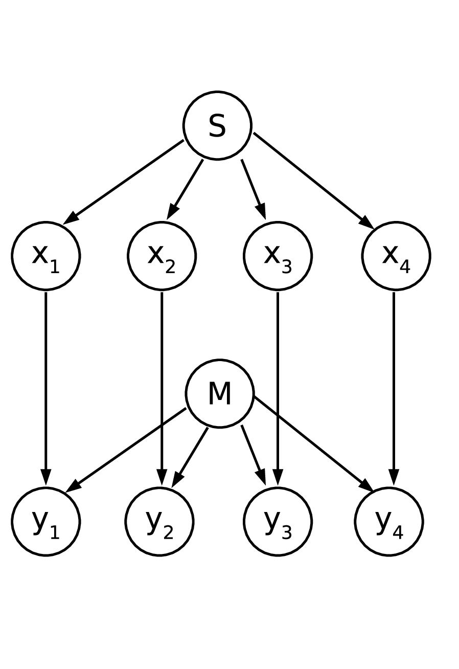
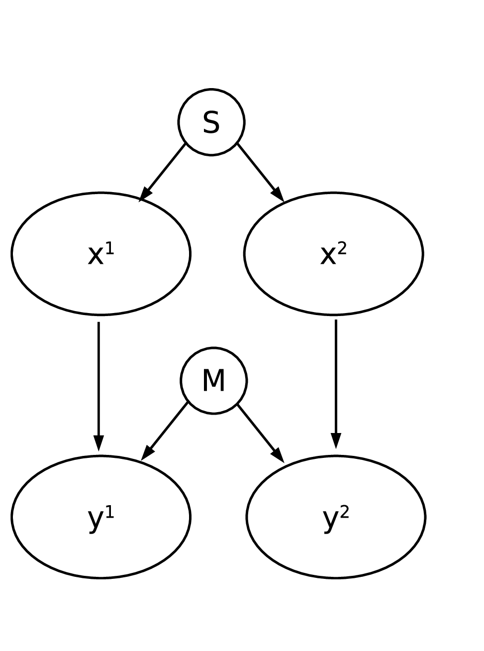
In analogy to the procedure above, we divide the string into and and use the same grouping for the -values. We then draw the causal graph in fig. 5 (right) showing causal relations between . Now we assume that and are not known, i.e., we don’t have access to the relevant properties of and . Thus we have to consider and as “hidden objects” (in analogy to hidden variables in the statistical setting). Therefore we have to apply the Markov condition to the causal structure in such a way that only the observed objects occur. One checks easily that d-separates and and d-separates and . Exhaustive search over all possible triples of subsets of shows that these are the only non-trivial d-separation conditions. We conclude
| (21) |
The most remarkable property of eq. (21) is that it is asymmetric with respect to exchanging the roles of and since, for instance, can be violated. Intuitively, the reason is that given , the knowledge of provides better insights into the properties of and than knowledge of would do, which can be an advantage when describing . The following example shows that this asymmetry can even be relevant for sample size provided that the probability space is large.
Let be a source that always generates the same string . Assume furthermore that is algorithmically random in the sense that . For sample size we then have . Let be a machine that randomly removes digits randomly either at the beginning or the end from its input string of length . By this procedure we obtain a string with from .
For sample size it is likely that and contain the last and the first digits of , respectively, or vice versa. This process is depicted in fig. 6 for and . Since the sample size is only two, the partition of the sample into two halves leads to single observations, i.e., and for .

In short-hand notation, and . We then have
but
which correctly lets us prefer the causal direction because these dependences violate the global algorithmic Markov condition in Theorem 3 when applied to a hypothetical graph where and are the outputs of the source and and are the outputs of a machine that has received and .
Even though the condition in eq. (21) does not explicitly contain the notion of complexities of Markov kernels it is closely related to the algorithmic independence of Markov kernels. To explain this, assume we would generate algorithmic dependences between and by adding an arrow or or by adding a common cause. Then would no longer d-separate from . The possible violation of eq. (21) could then be an observable result of the algorithmic dependences between the hidden objects and (and their statistical properties and , respectively).
3.3 Conditional density estimation on subsamples
Now we develop an inference rule that is even closer to the idea of checking algorithmic dependences of Markov kernels than condition (21), but still avoids the notion of Kolmogorov complexity of the “true” conditional distributions by using finite sample estimates instead. Before we explain the idea we mention two simpler approaches for doing so and describe their potential problems. It would be straightforward to apply Postulate 7 to the finite sample estimates of the conditionals. In particular, minimum description length (MDL) approaches [21] appear promising from the theoretical point of view due to their close relation to Kolmogorov complexity. We rephrase the minimum complexity estimator described by Barron and Cover [30]: Given a string-valued random variable and a sample drawn from , set
where runs over all probability densities on the probability space under consideration. If the data is sampled from a computable distribution, then converges in probability to [30]. Let us define a similar estimator for the conditional density . Could we reject the causal hypothesis after observing that and are mutually dependent? In the context of the true probabilities, we have argued that and represent independent mechanisms. However, for the estimators we do not see a justification for independence because the relative frequencies of the -values influence the estimation of and . This counter-argument becomes irrelevant only if the sample size is such that the complexities of the estimators coincide with the complexities of the true distributions. If we assume that the latter are typically uncomputable (because generic real numbers are uncomputable) this sample size will never be attained.
The general idea of MDL [21] also suggests the following causal inference principle: If we are given the data points with , consider the MDL estimators and . They define a joint distribution that we denote by (where we have dropped for convenience). The total description length
measures the complexity of the probabilistic model plus the complexity of the data, given the model. Then we compare to (defined correspondingly) and prefer the causal direction with the smaller value. However, it is not clear whether this kind of reasoning can be derived from the algorithmic Markov condition.
For this reason, we construct an inference rule that uses estimators in a more sophisticated way and whose justification is directly based on applying the algorithmic Markov condition to the resolution of ensembles. The idea of our strategy is that we do not use the full data set to estimate . Instead, we apply the estimator to a subsample of pairs that no longer carries significant information about the relative frequencies of -values in the full data set. As we will see below, this leads to algorithmically independent finite sample estimators for the Markov kernels if the causal hypothesis is correct.
Let be the causal structure that generated the data , with and after -fold i.i.d. sampling from . The resolution of the ensemble is the causal graph in fig. 7, left.
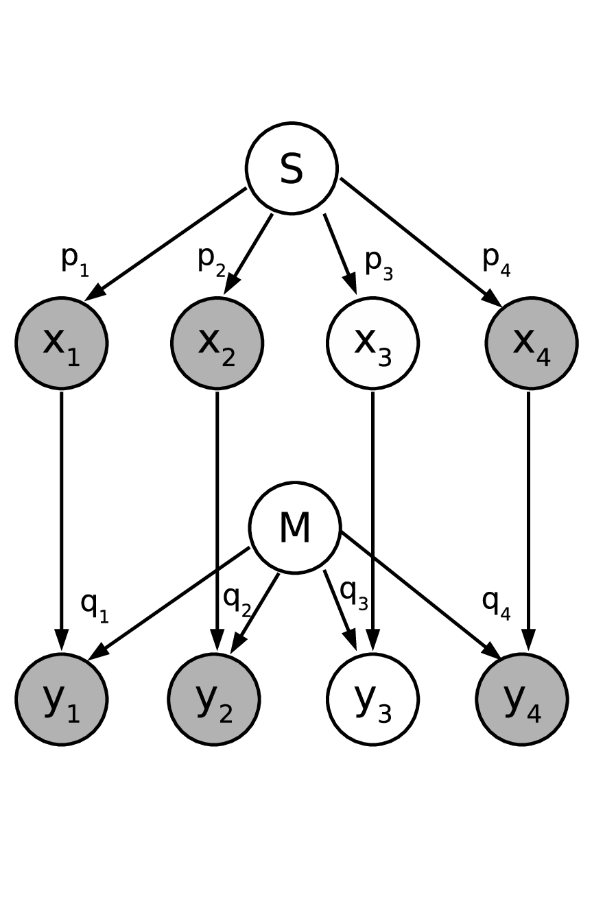
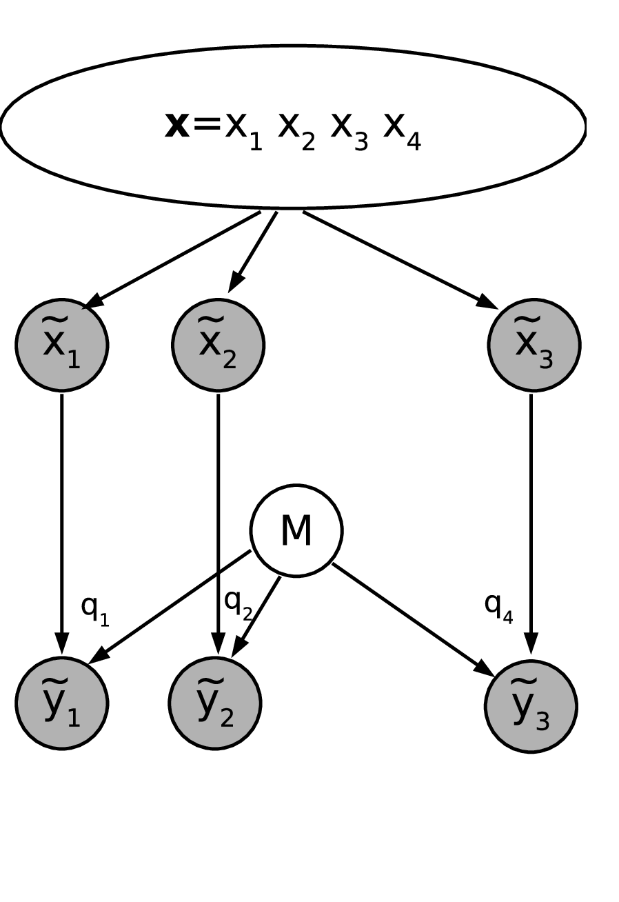
According to Postulate 6 there are mutually independent programs computing from the description of . Likewise, there are mutually independent programs computing from and . Assume we are given a rule how to generate a subsample of from . It is important that this selection rule does not refer to but only uses (as well as some random string as additional input) and that the selection can be performed by a program of length . Denote the subsample by
with . The above selection of indices defines also a subsample of -values
By construction, we have
Hence we can draw the causal structure depicted in fig. 7, right.
Let now be any string that is derived from by some program of length . may be the full description of relative frequencies or any computable density estimator , or some other description of interesting properties of the relative frequencies. Similarly, let be a description that is derived from by some simple algorithmic rule. The idea is that it is a computable estimator for the conditional distribution or any relevant property of the latter. Instead of estimating conditionals, one may also consider an estimator of the joint density of the subsample. We augment the causal structure in fig. 7, right, with and . The structure can be simplified by merging nodes in the same level and we obtain the structure in fig. 8.
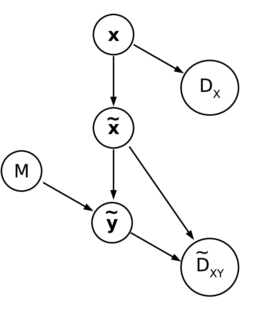
To derive testable implications of the causal hypothesis, we observe that every information between and is processed via . We thus have
| (22) |
which formally follows from the global Markov condition in Theorem 3. Using Lemma 8 and eq. (22) we conclude
| (23) |
The intention behind generating the subsample is to “blur” the distribution of . If we have a density estimator we try to choose the subsample such that the algorithmic mutual information between and is small. Otherwise we have not sufficiently blurred the distribution of . Then we apply an arbitrary conditional density estimator to the subsample. If there still is a non-negligible amount of mutual information between and , the causal hypothesis in fig. 5, left, cannot be true and we reject .
To show that the above procedure can also be applied to data sampled from uncomputable probability distributions, let and be uncomputable distributions on and uncomputable stochastic maps from to . Define a string-valued random variable with distribution as in Definition 5 and the conditional distribution of a string-valued variable by as in Definition 6 for strings . Let and as well as and be known up to an accuracy that is sufficient to distinguish between them. We assume that all this information (including ) is given as background knowledge, but and are unknown. Let , where is the estimated value of computed from the finite sample of size . Likewise, let be the estimated value of derived from the subsample of size . If is large enough (such that also is sufficiently large) we can estimate and , i.e, and with high probability. The most radical method to blur is to choose such that the empirical distribution of -values is uniform and the -values are lexicographically reordered (with some random ordering among the -values that correspond to the same -value). The only algorithmic information that then contains is the description of its length, i.e., bits. Hence we have
Assume now that . Then
provided that the estimation was correct. As shown at the end of Subsection 3.1, this is already possible for , i.e.,
which violates ineq. (23). The importance of this example lies in the fact that is not well-defined here because and both are uncomputable. Nevertheless, and have a computable aspect, i.e, the strings and characterizing them. Our strategy is therefore suitable to detect algorithmic dependences between computable features.
It is remarkable that the above scheme is general enough to include also strategies for very small sample sizes provided that the probability space is large. To describe an extreme case, we consider again the example with the truncated strings in fig. 6 with the role of and reversed. Let be a random variable whose value is always the constant string . Let be the mechanism that generates by truncating either the leftmost digits or the rightmost digits of (each with probability ). We denote these strings by and , respectively. Assume we have two observations , and , . We define a subsample by selecting only the first observation and . Then we define and . We observe that the mutual information between and is , while the mutual information between and is only . Given generic choices of , this violates condition (23) and we reject the causal hypothesis .
3.4 Plausible Markov kernels in time series
Time series are interesting examples of causal structures where the time order provides prior knowledge on the causal direction. Since there is a large number of them available from all scientific disciplines they can be useful to test causal inference rules on data with known ground truth. Let us consider the following example of a causal inference problem. Given a time series and the prior knowledge that it has been generated by a first order Markov process, but the direction is unknown. Formally, we are given observations corresponding to random variables such that the causal structure is either
| (24) |
or
| (25) |
where we have extended the series to infinity in both directions.
The question is whether the asymmetry of the joint distribution with respect to time inversion provides hints on the real time direction. Let us assume now that the graph (24) corresponds to the true time direction. Then the hope is that is simpler, in some reasonable sense, than . At first glance this seems to be a straightforward extension of the principle of plausible Markov kernel discussed in Subsection 3.1. However, there is a subtlety with the justification when we apply our ideas to stationary time series:
Recall that the principle of minimizing the total complexity of all Markov kernels over all potential causal directions has been derived from the independence of the true Markov kernels (remarks after Postulate 7). However, the algorithmic independence of and fails spectacularly because stationarity implies that these Markov kernels coincide and represent a causal mechanism that is constant in time. This shows that the justification of minimizing total complexity breaks down for stationary time series.
The following argument shows that not only the justification breaks down but also the principle as such: Consider the case where is the unique stationary distribution of the Markov kernel . Then we have
Because the forward time conditional describes uniquely the backward time conditional (via implying the description of the unique stationary marginal) the Kolmogorov complexity of the latter can exceed the complexity of the former only by a constant term.
We now focus on non-stationary time series. To motivate the general idea we first present an example described in [31]. Consider a random walk of a particle on starting at . In every time step the probability is to move one site to the right and to move to the left. Let with be the random variable describing the position after step . Then we have . The forward time conditional reads
To compute the backward time conditional we first compute which is given by the distribution of a Bernoulli experiment with steps. Let denote the number of right moves, i.e., is the number of left moves. With we thus obtain
Elementary calculations show
The forward time process is specified by the initial condition (given by ) and the transition probabilities (given by ). A priori, these two “objects” are mutually unrelated, i.e.,
On the other hand, the description of (the “initial condition” of the backward time process) alone already requires the specification of both and . The description of the “transition rule” refers only to . We thus have
Hence
The fact that the initial distribution of the hypothetical process
shares algorithmic information with the transition probabilities makes the hypothesis suspicious.
Resolving time series
We have seen that the algorithmic dependence between “initial condition” and “transition rule” of the backward time process (which would be surprising if it occurred for the forward time process) represents an asymmetry of non-stationary time-series with respect to time reflection. We will now discuss this asymmetry after resolving the statistical ensemble into individual observations.
Assume we are given instances of -tuples with that have been i.i.d. sampled from and are part of a time series that can be described by a first order stationary Markov process. Our resolution of a statistical ensemble generated by contained a source and a machine . The source generates -values and the machine generates -values from the input . The algorithmic independence of and was essential for the asymmetry between cause and effect described in Subsection 3.2. For the causal chain
we would therefore have machines generating the -value from . However, for stationary time-series all are the same machine. The causal structure of the resolution of the statistical ensemble for is shown in fig. 9, left.


This graph entails no independence constraint that is asymmetric with respect to reversing the time direction. To see this, recall that two DAGs entail the same set of independences if and only if they have the same skeleton (i.e. the corresponding undirected graphs coincide) and the same set of unshielded colliders (-structures), i.e., substructures where and are non-adjacent [1]. Fig. 9 has no such -structure and the skeleton is obviously symmetric with respect to time-inversion.
The initial part is, however, asymmetric (in agreement with the asymmetries entailed by fig. 5, left) and we have
This is just the finite-sample analogue of the statement that the initial distribution and the transition rule are algorithmically independent.
4 Decidable modifications of the inference rule
To use the algorithmic Markov condition in practical applications we have to replace it with computable notions of complexity. The following two subsections discuss two different directions along which practical inference rules can be developed.
4.1 Causal inference using symmetry constraints
We have seen that the algorithmic causal Markov condition implies that the the sum of the Kolmogorov complexities of the Markov kernels must be minimized over all possible causal graphs. In practical applications, it is natural to replace the minimization of Kolmogorov complexity with a decidable simplicity criterion even though this makes the relation to the theory developed so far rather vague. In this subsection we will describe an empirically decidable inference rule and show that the relation to Kolmogorov complexity of conditionals is closer than it may seem at first glance.
Moreover, the example below shows a scenario where the causal hypothesis can already be preferred to by comparing only the marginal distributions and and observing that a simple conditional leads from the former to the latter but no simple conditional leads into the opposite direction. The example will furthermore show why the identification of causal directions is often easier for probabilistic causal relations than for deterministic ones, a point that has also been pointed out by Pearl [1] in a different context.
Consider the discrete probability space . Given two distributions like the ones depicted in fig. 10 for . The marginal consists of sharp peaks of equal height at positions and also has modes centered at the same positions, but with greater width. We assume that can be obtained from by repeatedly applying a doubly stochastic matrix with for and for . The stochastic map thus defines a random walk and we have by assumption
for some .
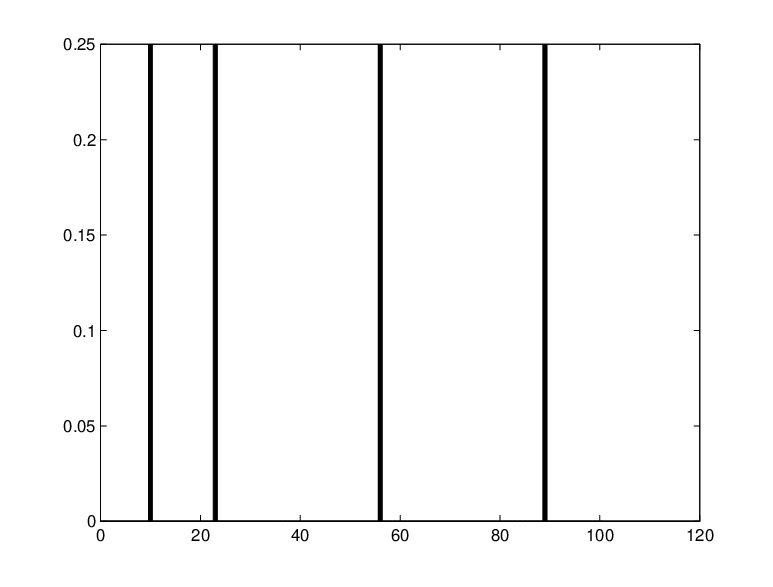

Now we ask which causal hypothesis is more likely: (1) has been obtained from by some stochastic map . (2) has been obtained from by some stochastic map . Our assumptions already contain an example that corresponds to the first hypothesis (). Clearly, there also exist maps for hypothesis (2). One example would be
| (27) |
i.e. has the probability vector in every column.
To describe in which sense is the simpler hypothesis we observe that in eq. (27) already contains the description of the positions whereas is rather simple. The Kolmogorov complexity of as chosen above is for a generic choice of the positions given by
where denotes equality up to a term that does not depend on . This is because different locations of the original peaks lead to different distributions and, conversely, every such is uniquely defined by describing the positions of the corresponding sharp peaks and .
However, we want to prove that also other choices of necessarily have high values of Kolmogorov complexity. To this end, we define a family of probability distributions given by equally high peaks at the positions and accordingly the smoothed probability distributions . We first need the following result.
Lemma 10 (average complexity of stochastic maps)
Let and be
two families of marginal distributions of and , respectively.
Moreover, let be a family of not necessarily different stochastic matrices with . Then
where the information that contains about the index is given by
denotes the random variable with values . Here, denotes the Shannon entropy and is computed in a similar way as using instead of .
Proof: The idea is to show that we need at least different stochastic matrices to achieve that the information exceeds by the amount . Using a standard argument rephrased below, the average complexity is therefore at least .
Assume, for instance, that all coincide. Then the usual data processing inequality [18] shows that applying the same matrix to the different distributions can never increase the information on the index , i.e., . To derive the lower bound on the number of different matrices required we define a partition of into sets for which the coincide. In other words, we have if and the matrices are chosen appropriately. We define a random variable whose value indicates that lies in the th equivalence class. The above “data processing argument” implies
| (28) |
Furthermore, we have
| (29) |
This is because both and cannot exceed because is the number of values can attain. Then we have:
The first equality follows because contains no additional information on (when is known) since it describes only from which equivalence class is taken. The second equality is a general rule for mutual information [18]. The inequality combines ineqs. (28) and (29). The last equality follows similar as the equalities in the first line. This shows that we need at least different matrices with . We have
where the first inequality holds because the exponential function is concave and the second is entailed by Kraft’s inequality. This yields
completing the proof.
To apply Lemma 10 to the above example we define families of distributions having their peaks at the positions and also their smoothed versions . Mixing all probability distributions will generate the entropy for because we then obtain the uniform distribution. Since we have assumed that can be obtained from by a doubly stochastic map, mixing all also yields the uniform distribution. Hence the difference between and is simply given by the average entropy difference
The Kolmogorov complexity required to map to is thus, on average over all , at least the entropy generated by the double stochastic random walk. Hence we have shown that a typical example of two distributions with peaks at arbitrary positions needs a process whose Kolmogorov complexity is at least the entropy difference.
One may ask why to consider distributions with several peaks even though the above result will formally also apply to distributions and with only one peak. The problem is that the statement “two distributions have a peak at the same position” does not necessarily make sense for empirical data. This is because the definition of variables is often chosen such that the distribution becomes centralized. The statement that multiple peaks occur on seemingly random positions seems therefore more sensible than the statement that one peak has been observed at a random position.
We have above used a finite number of discrete bins in order or keep the problem as much combinatorial as possible. In reality, we would rather expect a scenario like the one in fig. 11 where two distributions on have the same peaks, but the peaks in the one distribution have been smoothed, for example by an additive Gaussian noise.

As above, we would rather assume that is the cause of than vice versa since the smoothing process is simpler than any process that leads in the opposite direction. We emphasize that denoising is an operation that cannot be represented by a stochastic matrix, it is a linear operation that can be applied to the whole data set in order to reconstruct the original peaks. The statement is thus that no simple stochastic process leads in the opposite direction. To further discuss the rationale behind this way of reasoning we introduce another notion of simplicity that does not refer to Kolmogorov complexity. To this end, we introduce the notion of translation covariant conditional probabilities:
Definition 7 (translation covariance)
Let be two real-valued random variables.
A conditional distribution with density is called translation covariant if
Apart from this, we will also need the following well-known concept from statistical estimation theory [32]:
Definition 8 (Fisher information)
Let be a continuously differentiable
probability density of on . Then the Fisher information
is defined as
Then we have the following Lemma (see Lemma 1 in [33] showing the statement in a more general setting that involves also quantum stochastic maps):
Lemma 11 (monotonicity under covariant maps)
Let be a joint distribution such that is
translation covariant. Then
The intuition is that quantifies the degree to which a distribution is non-invariant with respect to translations and that no translation covariant process is able to increase this measure. The convolution with a Gaussian distribution with non-zero variance decreases the Fisher information. Hence there is never a translation invariant stochastic map in backward direction.
The argument above can easily be generalized in two respects. First, the argument works also with other quantities that are monotonous with respect to translation invariant stochastic maps. Second, we can also consider more general symmetries:
Definition 9 (general group covariance)
Let be random variables with equal range .
Let be a group of bijections
and and denoting
the random variables obtained by permuting the outcomes of the corresponding
random experiment according to .
Then we call a conditional -covariant if
It is easy to see that covariant stochastic maps define a quasi-order of probability distributions on by defining if there is a covariant stochastic map such that . This is transitive since the concatenation of covariant maps is again covariant.
If a -invariant measure (“Haar measure”) exists on we can easily define an information theoretic quantity that measures the degree of non-invariance with respect to :
Definition 10 (reference information)
Let be a distribution on and be a group of bijections on with Haar measure .
Then the reference information is given by:
The name “reference information” has been used in [34] in a slightly different context where this information occurred as the value of a physical system to communicate a reference system (e.g. spatial or temporal) where describes, for instance, translations in time or space. The quantity can easily be interpreted as mutual information if we introduce a -valued random variable whose values indicate which transformation has been applied. One can thus show that is non-increasing with respect to every -covariant map [34, 35].
The following model describes a link between inferring causal directions by preferring covariant conditionals to preferring directions with algorithmically independent Markov kernels. Consider first the probability space . We define the group , i.e., the additive group of integers modulo , acting on as bit-flips or identity. For any distribution on on , the reference information then measures the asymmetry with respect to bit-flips. For two distributions and we can have the situation that a -symmetric stochastic matrix leads from to , but only asymmetric stochastic maps convert into . Now we extend this idea to the group acting on strings of length by independent bit-flips. Assume we have a distribution on of the form in Definition 5 for some string and generate the distribution by applying to where
with . Then is -symmetric, but no -symmetric process leads backwards. This is because every such stochastic map would be asymmetric in a way that encodes , i.e., the map would have “to know” because has destroyed some amount of information about it.
4.2 Resource-bounded complexity
The problem that the presence or absence of mutual information is undecidable (when defined via Kolmogorov complexities) is similar to statistics, but also different in other respects. Let us first focus on the analogy. Given two real-valued random variables , it is impossible to show by finite sampling that they are statistically independent. is equivalent to for every pair of measurable functions. If we observe significant correlations between and for some previously defined pair, it is well-justified to reject independence. The same holds if such correlations are detected for in some previously defined, sufficiently small set of functions (cf. [36]). However, if this is not the case, we can never be sure that there is not some pair of arbitrarily complex functions that are correlated with respect to the true distribution. Likewise, if we have two strings and find no simple program that computes from this does not mean that there is no such a rule. Hence, we also have the statement that there can be an algorithmic dependence even though we do not find it.
However, the difference to the statistical situation is the following. Given that we have found functions yielding correlations it is only a matter of the statistical significance level whether this is sufficient to reject independence. For algorithmic dependences, we do not even have a decidable criterion to reject independence. Given that we have found a simple program that computes from , it still may be true that is small because there may also be a simple rule to generate (which would imply ) that we were not able to find. This shows that we can neither show dependence nor independence.
One possible answer to these problems is that Kolmogorov complexity is only an idealization of empirically decidable quantities. Developing this idealization only aims at providing hints in which directions we have to develop practical inference rules. Compression algorithms have already been developed that are intended to approximate, for instance, the algorithmic information of genetic sequences [37, 38]. Chen et al. [38] constructed a “conditional compression scheme” to approximate conditional Kolmogorov complexity and applied it to the estimation of the algorithmic mutual information between two genetic sequences. To evaluate to which extent methods of this kind can be used for causal inference using the algorithmic Markov condition is an interesting subject of further research.
It is also noteworthy that there is a theory on resource-bounded description complexity [19] where compressions of are only allowed if the decompression can be performed within a previously defined number of computation steps and on a tape of previously defined length. An important advantage of resource-bounded complexity is that it is computable. The disadvantage, on the other hand, is that the mathematical theory is more difficult. Parts of this paper have been developed by converting statements on statistical dependences into their algorithmic counterpart. The strong analogy between statistical and algorithmic mutual information occurs only for complexity with unbounded resources. For instance, the symmetry breaks down when replacing Kolmogorov complexity with resource-bounded versions [19]. Nevertheless, to develop a theory of inferred causation using resource-bounded complexity could be a challenge for the future. There are several reasons to believe that taking into account computational complexity can provide additional hints on the causal structure:
Bennett [39, 40, 41], for instance, has argued that the logical depth of an object echoes in some sense its history. The former is, roughly speaking, defined as follows. Let be a string that describes the object and be its shortest description. Then the logical depth of is the number of time steps that a parallel computing device requires to compute from . According to Bennett, large logical depth indicate that the object has been created by a process that consisted of many non-trivial steps. This would mean that there also is some causal information that follows from the time-resources required to compute a string from its shortest description.
The time-resources required to compute one observation from the other also plays a role in the discussion of causal inference rules in [31]. The paper presents a model where the conditional
can be efficiently computed, while computing
is NP-hard. This suggests that the computation time required to use information of the cause for the description of the effect can be different from the time needed to obtain information on the cause from the effect. However, the goal of the present paper was to describe asymmetries between cause and effect that even occur when computational complexity is ignored.
5 Conclusions
We have shown that our algorithmic causal Markov condition links algorithmic dependences between single observations with the underlying causal structure in the same way This is similar to the way the statistical causal Markov condition links statistical dependences among random variables to the causal structure. The algorithmic Markov condition has implications on different levels:
(1) In conventional causal inference one can drop the assumption that observations
have been generated by independent sampling from a constant joint distribution
of random variables . Algorithmic information theory thus replaces statistical causal inference with a probability-free formulation.
(2) Causal relations among individual objects can be inferred provided their shortest descriptions are sufficiently complex.
(3) New statistical causal inference rules follow because causal hypotheses are suspicious if the corresponding Markov kernels are algorithmically dependent.
Since algorithmic mutual information is uncomputable because Kolmogorov complexity is uncomputable, we have presented decidable inference rules that are motivated by the uncomputable idealization.
References
- [1] J. Pearl. Causality. Cambridge University Press, 2000.
- [2] P. Spirtes, C. Glymour, and R. Scheines. Causation, Prediction, and Search. Lecture Notes in Statistics. Springer, New York, 1993.
- [3] S. Lauritzen, A. Dawid, B. Larsen, and H.-G. Leimer. Independence properties of directed Markov fields. Networks, 20:491–505, 1990.
- [4] S. Lauritzen. Graphical Models. Clarendon Press, Oxford, New York, Oxford Statistical Science Series edition, 1996.
- [5] C. Meek. Strong completeness and faithfulness in Bayesian networks. Proceedings of the Conference in Artificial Intelligence and Statistics, pages 441–418, 1995.
- [6] D. Heckerman, C. Meek, and G. Cooper. A Bayesian approach to causal discovery. In C. Glymour and G. Cooper, editors, Computation, Causation, and Discovery, pages 141–165, Cambridge, MA, 1999. MIT Press.
- [7] Omnès, R. The interpretation of quantum mechanics. Princeton Series in Physics. Princeton University Press, 1994.
- [8] X. Sun, D. Janzing, and B. Schölkopf. Causal inference by choosing graphs with most plausible Markov kernels. In Proceedings of the 9th International Symposium on Artificial Intelligence and Mathematics, pages 1–11, Fort Lauderdale, FL, 2006.
- [9] X. Sun, D. Janzing, and B. Schölkopf. Causal reasoning by evaluating the complexity of conditional densities with kernel methods. Neurocomputing, 71:1248–1256, 2008.
- [10] Y. Kano and S. Shimizu. Causal inference using nonnormality. In Proceedings of the International Symposium on Science of Modeling, the 30th Anniversary of the Information Criterion, pages 261–270, Tokyo, Japan, 2003.
- [11] C.-H. Bennett, M. Li, and B. Ma. Chain letters and evolutionary histories. Scientific American, 288(6):76–81, 2003.
- [12] D. Hofheinz, J. Müller-Quade, and R. Steinwandt. On modelling IND-CCA security in cryptographic protocols. Proceedings of the 4th Central European Conference on Cryptology, Wartacrypt 2004.
- [13] R. Solomonoff. A preliminary report on a general theory of inducative inference. Technical report V-131, Report ZTB-138 Zator Co., 1960.
- [14] R. Solomonoff. A formal theory of inductive inference. Information and Control, Part II, 7(2):224–254, 1964.
- [15] A. Kolmogorov. Three approaches to the quantitative definition of information. Problems Inform. Transmission, 1(1):1–7, 1965.
- [16] G. Chaitin. On the length of prgrams for computing finire binary sequences. J. Assoc. Comput. Mach., 13:547–569, 1966.
- [17] G. Chaitin. A theory of program size formally identical to information theory. J. Assoc. Comput. Mach., 22:329–340, 1975.
- [18] T. Cover and J. Thomas. Elements of Information Theory. Wileys Series in Telecommunications, New York, 1991.
- [19] M. Li and P. Vitányi. An Introduction to Kolmogorov Complexity and its Applications. Springer, New York, 1997.
- [20] P. Gacs, J. Tromp, and P. Vitányi. Algorithmic statistics. IEEE Trans. Inf. Theory, 47(6):2443–2463, 2001.
- [21] P. Grünwald. The minimum description length principle. MIT Press, Cambridge, MA, 2007.
- [22] C.-H. Bennett, P. Gács, M. Li, P. Vitányi, and W. Zurek. Information distance. IEEE Trans. Inf. Th., IT-44:4:1407–1423, 1998.
- [23] M. Li, X. Chen, X. Li, B. Ma, and P. Vitányi. The similarity metric. IEEE Trans. Inf. Th., IT-50:12:3250–3264, 2004.
- [24] H. Reichenbach. The direction of time. Dover, 1999.
- [25] D. Deutsch. Quantum theory, the Church-Turing Principle and the universal quantum computer. Proceedings of the Royal Society, Series A(400):97–117, 1985.
- [26] M. Nielsen and I. Chuang. Quantum Computation and Quantum Information. Cambridge University Press, 2000.
- [27] D. Janzing and T. Beth. On the potential influnece of quantum noise on measuring effectiveness of drugs in clinical trials. Int. Journ. Quant. Inf., 4(2):347–364, 2006.
- [28] A. Milosavljević and J. Jurka. Discovery by minimal length encoding: a case study in molecular evolution. Machine Learning, 12:69–87, 1993.
- [29] J. Lemeire and E. Dirkx. Causal models as minimal descriptions of multivariate systems. Online preprint (not accessible any more).
- [30] A. Barron and T. Cover. Minimum complexity density estimation. IEEE Trans. Inf. Theory, 37(4):1034–1054, 1991.
- [31] D. Janzing. On causally asymmetric versions of Occam’s Razor and their relation to thermodynamics. http://arxiv.org/abs/0708.3411.
- [32] H. Cramér. Mathematical methods of statistics. Princeton University Press, Princeton, 1946.
- [33] D. Janzing and T. Beth. Quasi-order of clocks and their synchronism and quantum bounds for copying timing information. IEEE Trans. Inform. Theor., 49(1):230–240, 2003.
- [34] J. Vaccaro, F. Anselmi, H. Wiseman, and K. Jacobs. Complementarity between extractable mechanical work, accessible entanglement, and ability to act as a reference frame, under arbitrary superselection rules. http://arxiv.org/abs/quant-ph/0501121.
- [35] D. Janzing. Quantum thermodynamics with missing reference frames: Decompositions of free energy into non-increasing components. J. Stat. Phys., 125(3):757–772, 2006.
- [36] A. Gretton, R. Herbrich, A. Smola, O. Bousquet, and B. Schölkopf. Kernel methods for measuring independence. Journal of Machine Learning Research, 6:2075–2129, 2005.
- [37] S. Grumbach and F. Tahi. A new challenge for compression algorithms: genetic sequences. Information Processing & Management, 30(6), 1994.
- [38] X. Chen, Kwong X., and M. Li. A compression algorithm for DNA sequences and its applications in genome comparison. In RECOMB, page 107, 2000.
- [39] C.-H. Bennett. How to define complexity in physics and why. In W. Zurek, editor, Complexity, Entropy, and the Physics of Information, volume VIII of Santa Fee Studies of Complexity, pages 137–148. Adosin-Wesley, 1990.
- [40] C.-H. Bennett. On the nature and origin of complexity in discrete, homogeneous, locally-interacting systems. Foundations of Physics, 16(6):585–592, 1986.
- [41] C.-H. Bennett. Logical depth and physical complexity. In R. Herken, editor, The Universal Turing Machine - a Half-Century Survey, pages 227–257. Oxford University Press, 1988.