On sensitive dependence on initial conditions and existence of physical measure for -flowsThanks: Author was partially supported by FAPERJ (Rio de Janeiro), FAPESB (Bahia), CNPq and PRONEX-Dynamical Systems (Brazil).
Abstract.
After reviewing known results on sensitiveness and also on robustness of attractors together with observations on their proofs, we show that for attractors of three-dimensional flows, robust chaotic behavior (meaning sensitiveness to initial conditions for the past as well for the future for all nearby flows) is equivalent to the existence of certain hyperbolic structures. These structures, in turn, are associated to the existence of physical measures. In short in low dimensions, robust chaotic behavior for smooth flows ensures the existence of a physical measure.
Key words and phrases:
sensitive dependence on initial conditions, physical measure, singular-hyperbolicity, expansiveness, robust attractor, robust chaotic flow, positive Lyapunov exponent1991 Mathematics Subject Classification
Primary: 37D25; Secondary: 37D30, 37D45.1. Introduction
The development of the theory of dynamical systems has shown that models involving expressions as simple as quadratic polynomials (as the logistic family or Hénon attractor, see e.g.[8] for a gentle introduction), or autonomous ordinary differential equations with a hyperbolic equilibrium of saddle-type accumulated by regular orbits, as the Lorenz flow (see e.g. [12, 30, 2]), exhibit sensitive dependence on initial conditions, a common feature of chaotic dynamics: small initial differences are rapidly augmented as time passes, causing two trajectories originally coming from practically indistinguishable points to behave in a completely different manner after a short while. Long term predictions based on such models are unfeasible since it is not possible to both specify initial conditions with arbitrary accuracy and numerically calculate with arbitrary precision. For an introduction to these notions see [8, 28].
Formally the definition of sensitivity is as follows for a flow on some compact manifold : a -invariant subset is sensitive to initial conditions or has sensitive dependence on initial conditions, or simply chaotic if, for every small enough and , and for any neighborhood of , there exists and such that and are -apart from each other: . See Figure 1. An analogous definition holds for diffeomorphism of some manifold, taking and setting in the previous definition.

Using some known results on robustness of attractors from Mañé [18] and Morales, Pacifico and Pujals [21] together with observations on their proofs, we show that for attractors of three-dimensional flows, robust chaotic behavior (in the above sense of sensitiveness to initial conditions) is equivalent to the existence of certain hyperbolic structures. These structures, in turn, are associated to the existence of physical measures. In short in low dimensions, robust chaotic behavior ensures the existence of a physical measure.
2. Preliminary notions
Here and throughout the text we assume that is a three-dimensional compact connected manifold without boundary endowed with some Riemannian metric which induces a distance denoted by and a volume form which we name Lebesgue measure or volume. For any subset of we denote by the (topological) closure of .
We denote by the set of smooth vector fields on endowed with the topology. Given we denote by , with , the flow generated by the vector field . Since we assume that is a compact manifold the flow is defined for all time. Recall that the flow is a family of diffeomorphisms satisfying the following properties:
- (1)
is the identity map of ;
- (2)
for all ,
and it is generated by the vector field if
- 3
for all and .
We say that a compact -invariant set is isolated if there exists a neighborhood of such that . A compact invariant set is attracting if equals for some neighborhood of satisfying , for all . In this case the neighborhood is called an isolating neighborhood of . Note that is in general different from , but for an attracting set the extra condition for ensures that every attracting set is also isolated. We say that is transitive if is the closure of both and for some . An attractor of is a transitive attracting set of and a repeller is an attractor for . We say that is a proper attractor or repeller if .
An equilibrium (or singularity) for is a point such that for all , i.e. a fixed point of all the flow maps, which corresponds to a zero of the associated vector field : . An orbit of is a set for some . A periodic orbit of is an orbit such that for some minimal . A critical element of a given vector field is either an equilibrium or a periodic orbit.
We recall that a -invariant probability measure is a probability measure satisfying for all and measurable . Given an invariant probability measure for a flow , let be the the (ergodic) basin of , i.e., the set of points satisfying for all continuous functions
We say that is a physical (or SRB) measure for if has positive Lebesgue measure: .
The existence of a physical measures for an attractor shows that most points in a neighborhood of the attractor have well defined long term statistical behavior. So, in spite of chaotic behavior preventing the exact prediction of the time evolution of the system in practical terms, we gain some statistical knowledge of the long term behavior of the system near the chaotic attractor.
3. Chaotic systems
We distinguish between forward and backward sensitive dependence on initial conditions. We say that an invariant subset for a flow is future chaotic with constant if, for every and each neighborhood of in the ambient manifold, there exists and such that . Analogously we say that is past chaotic with constant if is future chaotic with constant for the flow generated by . If we have such sensitive dependence both for the past and for the future, we say that is chaotic. Note that in this language sensitive dependence on initial conditions is weaker than chaotic, future chaotic or past chaotic conditions.
An easy consequence of chaotic behavior is that it prevents the existence of sources or sinks, either attracting or repelling equilibria or periodic orbits, inside the invariant set . Indeed, if is future chaotic (for some constant ) then, were it to contain some attracting periodic orbit or equilibrium, any point of such orbit (or equilibrium) would admit no point in a neighborhood whose orbit would move away in the future. Likewise, reversing the time direction, a past chaotic invariant set cannot contain repelling periodic orbits or repelling equilibria. As an almost reciprocal we have the following.
Lemma 1.
If is a compact isolated proper subset for with isolating neighborhood and is not future chaotic (respective not past chaotic), then (respective ) has non-empty interior.
Proof.
If is not future chaotic, then for every there exists some point and a neighborhood of such that for all and each . If we choose (we note that if then would be open and closed, and so, by connectedness of , would not be a proper subset), then we deduce that , that is, for all , hence . Analogously if is not past chaotic, just by reversing the time direction. ∎
In particular if an invariant and isolated set with isolating neighborhood is given such that the volume of both and is zero, then is chaotic.
Sensitive dependence on initial conditions is part of the definition of chaotic system in the literature, see e.g. [8]. It is an interesting fact that sensitive dependence is a consequence of another two common features of most systems considered to be chaotic: existence of a dense orbit and existence of a dense subset of periodic orbits.
Proposition 1.
A compact invariant subset for a flow with a dense subset of periodic orbits and a dense (regular and non-periodic) orbit is chaotic.
4. Lack of sensitiveness for flows on surfaces
We recall the following celebrated result of Mauricio Peixoto in [25, 26] (and for a more detailed exposition of this results and sketch of the proof see [12]) built on previous work of Poincaré [27] and Andronov and Pontryagin [1], that characterizes structurally stable vector fields on compact surfaces.
Theorem 1 (Peixoto).
A vector field, , on a compact surface is structurally stable if, and only if:
- (1)
the number of critical elements is finite and each is hyperbolic;
- (2)
there are no orbits connecting saddle points;
- (3)
the non-wandering set consists of critical elements alone.
Moreover if is orientable, then the set of structurally stable vector fields is open and dense in .
In particular, this implies that for a structurally stable vector field on there is an open and dense subset of such that the positive orbit of converges to one of finitely many attracting equilibria. Therefore no sensitive dependence on initial conditions arises for an open and dense subset of all vector fields in orientable surfaces.
The extension of Peixoto’s characterization of structural stability for flows, , on non-orientable surfaces is known as Peixoto’s Conjecture, and up until now it has been proved for the projective plane [23], the Klein bottle [19] and , the torus with one cross-cap [13]. Hence for these surfaces we also have no sensitiveness to initial conditions for most vector fields.
This explains in part the great interest attached to the Lorenz attractor which was one of the first examples of sensitive dependence on initial conditions.
5. Robustness and volume hyperbolicity
Related to chaotic behavior is the notion of robust dynamics. We say that an attracting set for a -flow and some open subset is robust if there exists a neighborhood of in such that is transitive for every .
The following result obtained by Morales, Pacifico and Pujals in [21] characterizes robust attractors for three-dimensional flows.
Theorem 2.
Robust attractors for flows containing equilibria are singular-hyperbolic sets for .
We remark that robust attractors cannot be approximated by vector fields presenting either attracting or repelling periodic points. This implies that, on -manifolds, any periodic orbit inside a robust attractor is hyperbolic of saddle-type.
We now define the concept of singular-hyperbolicity. A compact invariant set of is partially hyperbolic if there are a continuous invariant tangent bundle decomposition and constants such that
- •
-dominates , i.e. for all and for all
(5.1) - •
is -contracting: for all and for all .
For and we let be the absolute value of the determinant of the linear map . We say that the sub-bundle of the partial hyperbolic set is -volume expanding if
for every and .
We say that a partially hyperbolic set is singular-hyperbolic if its singularities are hyperbolic and it has volume expanding central direction.
A singular-hyperbolic attractor is a singular-hyperbolic set which is an attractor as well: an example is the (geometric) Lorenz attractor presented in [17, 11]. Any equilibrium of a singular-hyperbolic attractor for a vector field is such that has only real eigenvalues satisfying the same relations as in the Lorenz flow example:
| (5.2) |
which we refer to as Lorenz-like equilibria. We recall that an compact -invariant set is hyperbolic if the tangent bundle over splits into three -invariant subbundles, where is uniformly contracted, is uniformly expanded, and is the direction of the flow at the points of . It is known, see [21], that a partially hyperbolic set for a three-dimensional flow, with volume expanding central direction and without equilibria, is hyperbolic. Hence the notion of singular-hyperbolicity is an extension of the notion of hyperbolicity.
Recently in a joint work with Pacifico, Pujals and Viana [3] the following consequence of transitivity and singular-hyperbolicity was proved.
Theorem 3.
Let be a singular-hyperbolic attractor of a flow on a three-dimensional manifold. Then supports a unique physical probability measure which is ergodic and its ergodic basin covers a full Lebesgue measure subset of the topological basin of attraction, i.e. Lebesgue mod . Moreover the support of is the whole attractor .
It follows from the proof in [3] that the singular-hyperbolic attracting set for all which are -close enough to admits finitely many physical measures whose ergodic basins cover except for a zero volume subset.
5.1. Absence of sinks and sources nearby
The proof of Theorem 2 given in [21] uses several tools from the theory of normal hyperbolicity developed first by Mañé in [18] together with the low dimension of the flow. Indeed, going through the proof in [21] we can see that the arguments can be carried through assuming that
- (1)
is an attractor for with isolating neighborhood such that every equilibria in is hyperbolic with no resonances;
- (2)
there exists a neighborhood of such that for all every periodic orbit and equilibria in is hyperbolic of saddle-type.
The condition on the equilibria amounts to restricting the possible three-dimensional vector fields in the above statement to an open a dense subset of all vector fields. Indeed, the hyperbolic and no-resonance condition on a equilibrium means that:
- •
either if the eigenvalues of are and ;
- •
or has only real eigenvalues with different norms.
Indeed, conditions (1) and (2) ensure that no bifurcations of periodic orbits or equilibria leading to sinks or sources are allowed for any nearby flow in . This implies, by now standard arguments, that the flow on must have a dominated splitting which is volume hyperbolic: both subbundles of the splitting must contract/expand volume. For a -dimensional flow one of the subbundles is one-dimensional, and so we deduce singular-hyperbolicity either for or for . If has no equilibria, then is uniformly hyperbolic. Otherwise, it follows from the arguments in [21] that all singularities of are Lorenz-like and this shows that must be singular-hyperbolic for .
We note that the second condition above is a consequence of any one of the following assumptions on :
- robust chaoticity:
-
for every the maximal invariant subset is chaotic;
- zero volume and future chaoticity:
-
for every the maximal invariant subset has zero volume and is future chaotic;
- zero volume and robust positive Lyapunov exponent:
-
for every the maximal invariant subset has zero volume and there exists a full Lebesgue measure subset of such that
(5.3)
Theorem 4.
Robust attractors for surface diffeomorphisms are hyperbolic.
also follows from the absence of sinks and sources for all close diffeomorphisms in a neighborhood of the attractor.
Extensions of these results to higher dimensions for diffeomorphisms, by Bonatti, Díaz and Pujals in [6], show that robust transitive sets always admit a volume hyperbolic splitting of the tangent bundle. Vivier in [31] extends previous results of Doering [9] for flows, showing that a robustly transitive vector field on a compact boundaryless -manifold, with , admits a global dominated splitting. Metzger and Morales extend the arguments in [21] to homogeneous vector fields (inducing flows allowing no bifurcation of critical elements, i.e. no modification of the index of periodic orbits or equilibria) in higher dimensions leading to the concept of -sectional expanding attractor in [20].
5.2. Robust chaoticity, volume hyperbolicity and physical measure
The preceding observations allows us to deduce that robust chaoticity is a sufficient conditions for singular-hyperbolicity of a generic attractor.
Corollary 1.
Let be an attractor for such that every equilibrium in its trapping region is hyperbolic with no resonances. Then is singular-hyperbolic if, and only if, is robustly chaotic.
This means that if we can show that arbitrarily close orbits, in an isolating neighborhood of an attractor, are driven apart, for the future as well as for the past, by the evolution of the system, and this behavior persists for all nearby vector fields, then the attractor is singular-hyperbolic.
To prove the necessary condition on Corollary 1 we use the concept of expansiveness for flows, and through it show that singular-hyperbolic attractors for -flows are robustly expansive and, as a consequence, robustly chaotic also. This is done in the last Section 6.
We recall the following conjecture of Viana, presented in [29]
Conjecture 1.
If an attracting set of smooth map/flow has a non-zero Lyapunov exponent at Lebesgue almost every point of its isolated neighborhood (i.e. it satisfies (5.3) with ), then it admits some physical measure.
From the preceding results and observations we can give a partial answer to this conjecture for -flows in the following form.
Corollary 2.
Let be an attractor for a flow such that
- •
the divergence of is negative in ;
- •
the equilibria in are hyperbolic with no resonances;
- •
there exists a neighborhood of in such that for one has (5.3) almost everywhere in .
Then there exists a neighborhood of in and a dense subset such that
- (1)
is singular-hyperbolic for all ;
- (2)
there exists a physical measure supported in for all .
Indeed, item (2) above is a consequence of item (1), the denseness of in in the topology, together with Theorem 3 and the observation following its statement.
6. Expansive systems
Here we explain why robust chaotic behavior necessarily follows from singular-hyperbolicity in an attractor, completing the proof of Corollary 1. For this we need the concept and some properties of expansiveness for flows.
A concept related to sensitiveness is that of expansiveness, which roughly means that points whose orbits are always close for all time must coincide. The concept of expansiveness for homeomorphisms plays an important role in the study of transformations. Bowen and Walters [7] gave a definition of expansiveness for flows which is now called C-expansiveness citeKS79. The basic idea of their definition is that two points which are not close in the orbit topology induced by can be separated at the same time even if one allows a continuous time lag — see below for the technical definitions. The equilibria of C-expansive flows must be isolated [7, Proposition 1] which implies that the Lorenz attractors and geometric Lorenz models are not C-expansive.
Keynes and Sears introduced [15] the idea of restriction of the time lag and gave several definitions of expansiveness weaker than C-expansiveness. The notion of K-expansiveness is defined allowing only the time lag given by an increasing surjective homeomorphism of . Komuro [16] showed that the Lorenz attractor and the geometric Lorenz models are not K-expansive. The reason for this is not that the restriction of the time lag is insufficient, but that the topology induced by is unsuited to measure the closeness of two points in the same orbit.
Taking this fact into consideration, Komuro [16] gave a definition of expansiveness suitable for flows presenting equilibria accumulated by regular orbits. This concept is enough to show that two points which do not lie on a same orbit can be separated.
Let be the set of all continuous functions and let us write for the subset of all such that . We define
and
A flow is C-expansive (K-expansive respectively) on an invariant subset if for every there exists such that if and for some (respectively ) we have
| (6.1) |
then .
We say that the flow is expansive on if for every there is such that for and some (note that now we do not demand that be fixed by ) satisfying (6.1), then we can find such that .
Observe that expansiveness on implies sensitive dependence on initial conditions for any flow on a manifold with dimension at least 2. Indeed if satisfy the expansiveness condition above with equal to the identity and we are given a point and a neighborhood of , then taking (which always exists since we assume that is not one-dimensional) there exists such that . The same argument applies whenever we have expansiveness on an -invariant subset of containing a dense regular orbit of the flow.
Clearly C-expansive K-expansive expansive by definition. When a flow has no fixed point then C-expansiveness is equivalent to K-expansiveness [22, Theorem A]. In [7] it is shown that on a connected manifold a C-expansive flow has no fixed points. The following was kindly communicated to us by Alfonso Artigue from IMERL, the proof can be found in [2].
Proposition 2.
A flow is C-expansive on a manifold if, and only if, it is K-expansive.
We will see that singular-hyperbolic attractors are expansive. In particular, the Lorenz attractor and the geometric Lorenz examples are all expansive and sensitive to initial conditions. Since these families of flows exhibit equilibria accumulated by regular orbits, we see that expansiveness is compatible with the existence of fixed points by the flow.
6.1. Singular-hyperbolicity and expansiveness
Theorem 5.
Let be a singular-hyperbolic attractor of . Then is expansive.
The reasoning is based on analyzing Poincaré return maps of the flow to a convenient (-adapted) cross-section. We use the family of adapted cross-sections and corresponding Poincará maps , whose Poincaré time is large enough, obtained assuming that the attractor is singular-hyperbolic. These cross-sections have a co-dimension foliation, which are dynamically defined, whose leaves are uniformly contracted and invariant under the Poincaré maps. In addition is uniformly expanding in the transverse direction and this also holds near the singularities.
From here we argue by contradiction: if the flow is not expansive on , then we can find a pair of orbits hitting the cross-sections infinitely often on pairs of points uniformly close. We derive a contradiction by showing that the uniform expansion in the transverse direction to the stable foliation must take the pairs of points apart, unless one orbit is on the stable manifold of the other.
This argument only depends on the existence of finitely many Lorenz-like singularities on a compact partially hyperbolic invariant attracting subset , with volume expanding central direction, and of a family of adapted cross-sections with Poincaré maps between them, whose derivative is hyperbolic. It is straightforward that if these conditions are satisfied for a flow of , then the same conditions hold for all nearby flows and for the maximal invariant subset with the same family of cross-sections which are also adapted to (as long as is -close enough to ).
Corollary 3.
A singular-hyperbolic attractor is robustly expansive, that is, there exists a neighborhood of in such that is expansive for each , where is an isolating neighborhood of .
Indeed, since transversality, partial hyperbolicity and volume expanding central direction are robust properties, and also the hyperbolicity of the Poincaré maps depends on the central volume expansion, all we need to do is to check that a given adapted cross-section to is also adapted to for every sufficiently close to . But and are close in the Hausdorff distance if and are close in the distance, by the following elementary result.
Lemma 2.
Let be an isolated set of , . Then for every isolating block of and every there is a neighborhood of in such that and for all .
Thus, if is an adapted cross-section we can find a -neighborhood of in such that is still adapted to every flow generated by a vector field in .
6.2. Singular-hyperbolicity and chaotic behavior
We already know that expansiveness implies sensitive dependence on initial conditions. An argument with the same flavor as the proof of expansiveness provides the following, whose proof also sketch in the following Section 7.2. See also [4] for a different approach to sensitiveness.
Theorem 6.
A singular-hyperbolic isolated set is robustly chaotic, i.e. there exists a neighborhood of in such that is chaotic for each , where is an isolating neighborhood of .
This completes the argument proving that robust chaoticity is a necessary property of singular-hyperbolicity, in Corollary 1.
7. Sketch of the proof of expansiveness and of chaotic behavior
7.1. Adapted cross-sections and Poincaré maps
To help explain the ideas of the proofs we give here a few properties of Poincaré maps, that is, continuous maps of the form between cross-sections and of the flow near a singular-hyperbolic set. We always assume that the Poincaré time is large enough as explained in what follows.
We assume that is a compact invariant subset for a flow such that is a singular-hyperbolic attractor. Then every equilibrium in is Lorenz-like.
7.1.1. Stable foliations on cross-sections
We start recalling standard facts about uniformly hyperbolic flows from e.g. [14].
An embedded disk is a (local) strong-unstable manifold, or a strong-unstable disk, if tends to zero exponentially fast as , for every . Similarly, is called a (local) strong-stable manifold, or a strong-stable disk, if exponentially fast as , for every . It is well-known that every point in a uniformly hyperbolic set possesses a local strong-stable manifold and a local strong-unstable manifold which are disks tangent to and at respectively with topological dimensions and respectively. Considering the action of the flow we get the (global) strong-stable manifold
and the (global) strong-unstable manifold
for every point of a uniformly hyperbolic set. These are immersed submanifolds with the same differentiability of the flow. We also consider the stable manifold and unstable manifold for in a uniformly hyperbolic set, which are flow invariant.
Now we recall classical facts about partially hyperbolic systems, especially existence of strong-stable and center-unstable foliations. The standard reference is [14].
We have that is a singular-hyperbolic isolated set of with invariant splitting with . Let be a continuous extension of this splitting to a small neighborhood of . For convenience we take to be forward invariant. Then may be chosen invariant under the derivative: just consider at each point the direction formed by those vectors which are strongly contracted by for positive . In general is not invariant. However we can consider a cone field around it on
which is forward invariant for :
| (7.1) |
Moreover we may take arbitrarily small, reducing if necessary. For notational simplicity we write and for and in all that follows.
From the standard normal hyperbolic theory, there are locally strong-stable and center-unstable manifolds, defined at every regular point and which are embedded disks tangent to and , respectively. Given any define the strong-stable manifold and the stable-manifold as for an hyperbolic flow (see the beginning of this section).
Denoting , where is the direction of the flow at , it follows that
We fix once and for all. Then we call the local strong-stable manifold and the local center-unstable manifold of .
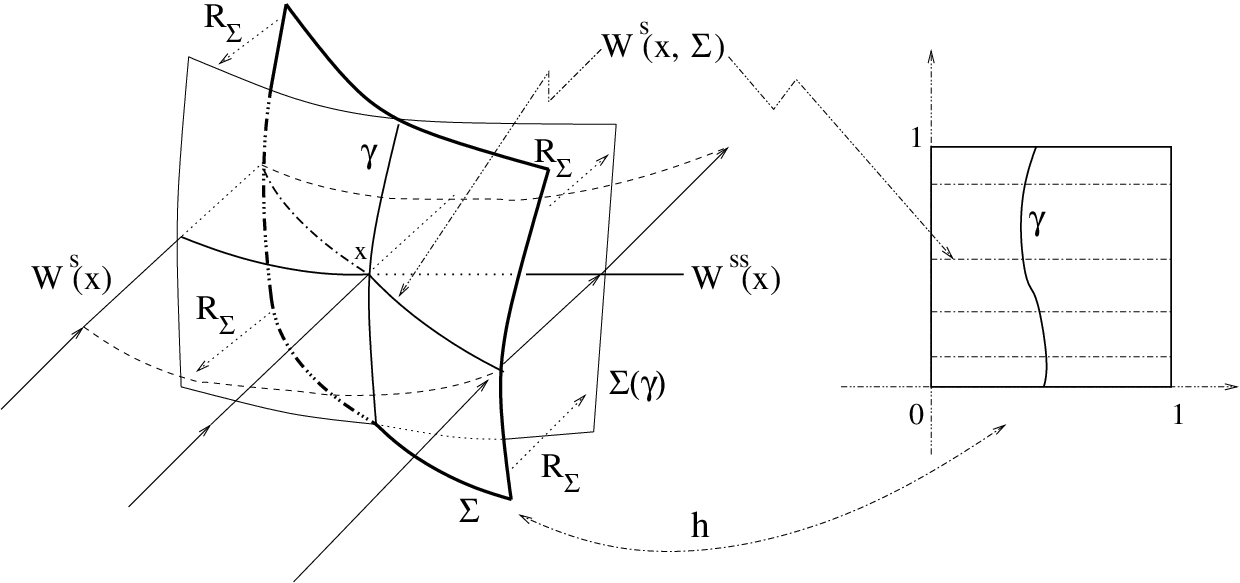
Now let be a cross-section to the flow, that is, a embedded compact disk transverse to : at every point we have (recall that is the one-dimensional subspace ). For every we define to be the connected component of that contains . This defines a foliation of into co-dimension sub-manifolds of class .
Given any cross-section and a point in its interior, we may always find a smaller cross-section also with in its interior and which is the image of the square by a diffeomorphism that sends horizontal lines inside leaves of . In what follows we assume that cross-sections are of this kind, see Figure 2.
We also assume that each cross-section is contained in , so that every is such that .
On the one hand is usually not differentiable if we assume that is only of class , see e.g. [24]. On the other hand, assuming that the cross-section is small with respect to , and choosing any curve crossing transversely every leaf of , we may consider a Poincaré map
with Poincaré time close to zero, see Figure 2. This is a homeomorphism onto its image, close to the identity, such that . So, identifying the points of with their images under this homeomorphism, we pretend that indeed .
7.1.2. Hyperbolicity of Poincaré maps
Let be a small cross-section to and let be a Poincaré map to another cross-section (possibly ). Here needs not correspond to the first time the orbits of encounter .
The splitting over induces a continuous splitting of the tangent bundle to (and analogously for ), defined by
| (7.2) |
We now show that if the Poincaré time is sufficiently large then (7.2) defines a hyperbolic splitting for the transformation on the cross-sections restricted to .
Proposition 3.
Let be a Poincaré map as before with Poincaré time . Then at every and at every .
Moreover for every given there exists such that if at every point, then
Given a cross-section , a positive number , and a point , we define the unstable cone of width at by
| (7.3) |
Let be any small constant. In the following consequence of Proposition 3 we assume the neighborhood has been chose sufficiently small.
Corollary 4.
For any as in Proposition 3, with , and any , we have and
As usual a curve is the image of a compact interval by a map. We use to denote its length. By a cu-curve in we mean a curve contained in the cross-section and whose tangent direction is contained in the unstable cone for all . The next lemma says that the length of cu-curves linking the stable leaves of nearby points must be bounded by the distance between and .
Lemma 3.
Let us we assume that has been fixed, sufficiently small. Then there exists a constant such that, for any pair of points , and any cu-curve joining to some point of , we have .
Here is the intrinsic distance in the surface , that is, the length of the shortest smooth curve inside connecting two given points in .
In what follows we take in Proposition 3 for .
7.1.3. Adapted cross-sections
Now we exhibit stable manifolds for Poincaré transformations . The natural candidates are the intersections we introduced previously. These intersections are tangent to the corresponding sub-bundle and so, by Proposition 3, they are contracted by the transformation. For our purposes it is also important that the stable foliation be invariant:
| (7.4) |
In order to have this we restrict our class of cross-sections whose center-unstable boundary is disjoint from . Recall that we are considering cross-sections that are diffeomorphic to the square , with the horizontal lines being mapped to stable sets . The stable boundary is the image of . The center-unstable boundary is the image of . The cross-section is -adapted if
where is the intrinsic distance in , see Figure 3.

Lemma 4.
Let be a regular point, that is, such that . There exists such that there exists a -adapted cross-section at .
We are going to show that if the cross-sections are adapted, then we have the invariance property (7.4). Given we set the domain of the return map from to .
Lemma 5.
Given and -adapted cross-sections and , there exists such that if defined by is a Poincaré map with time , then
- (1)
for every , and also
- (2)
for every , and .
Clearly we may choose so that all the properties of the Poincaré maps obtained up to here are valid for return times greater than .
7.2. The proof of expansiveness
Here we sketch the proof of Theorem 5. The proof is by contradiction: let us suppose that there exist , a sequence , a sequence of functions and sequences of points such that
| (7.5) |
but
| (7.6) |
The main step of the proof is a reduction to a forward expansiveness statement about Poincaré maps which we state in Theorem 7 below.
We are going to use the following observation: there exists some regular (i.e. non-equilibrium) point which is accumulated by the sequence of -limit sets . To see that this is so, start by observing that accumulation points do exist, since is compact. Moreover, if the -limit sets accumulate on a singularity then they also accumulate on at least one of the corresponding unstable branches which, of course, consists of regular points. We fix such a once and for all. Replacing our sequences by subsequences, if necessary, we may suppose that for every there exists such that .
Let be a -adapted cross-section at , for some small . Reducing (but keeping the same cross-section) we may ensure that is in the interior of the subset
By definition, returns infinitely often to the neighborhood of which, on its turn, is close to . Thus dropping a finite number of terms in our sequences if necessary, we have that the orbit of intersects infinitely many times. Let be the time corresponding to the th intersection.
Replacing , , , and by , , , and , we may suppose that , while preserving both relations (7.5) and (7.6). Moreover there exists a sequence , with such that
| (7.7) |
for all , where is given by Proposition 3 and is given by Lemma 5.
Theorem 7.
Given there exists such that if and satisfy
- (a):
-
there exist such that
- (b):
-
, for all and some ;
then there exists for some such that .
The proof of Theorem 7 will not be given here, and can be found in [3]. We explain why this implies Theorem 5. We are going to use the following observation.
Lemma 6.
There exist small and , depending only on the flow, such that if are points in satisfying and , with away from any equilibria of , then
This is a direct consequence of the fact that the angle between and the flow direction is bounded from zero which, on its turn, follows from the fact that the latter is contained in the center-unstable sub-bundle .
We fix as in (7.6) and then consider as given by Theorem 7. Next, we fix such that and , and apply Theorem 7 to and and . Hypothesis (a) in the theorem corresponds to (7.7) and, with these choices, hypothesis (b) follows from (7.5). Therefore we obtain that . Equivalently there is such that . Condition (7.6) then implies that . Hence since strong-stable manifolds are expanded under backward iteration, there exists maximum such that
for all , see Figure 4. Moreover for some so that is close to cross-section of the flow which we can assume is uniformly bounded away from the equilibria, and then we can assume that for . Since is maximum
for , because for .

7.3. Singular-hyperbolicity and chaotic behavior
Here we explain why singular-hyperbolic attractors, like the Lorenz attractor, are necessarily robustly chaotic.
of Theorem 6.
The assumption of singular-hyperbolicity on an isolated proper subset with isolating neighborhood ensures that the maximal invariant subsets for all nearby flows are also singular-hyperbolic. Therefore to deduce robust chaotic behavior in this setting it is enough to show that a proper isolated invariant compact singular-hyperbolic subset is chaotic.
Let be a singular-hyperbolic isolated proper subset for a flow. Then there exists a strong-stable manifold through each of its points . We claim that this implies that is past chaotic. Indeed, assume by contradiction that we can find such that and for every , for some small . Then, because is uniformly contracted by the flow in positive time, there exists such that
for all , a contradiction since . Hence for any given small we can always find a point arbitrarily close to (it is enough to choose is the strong-stable manifold of ) such that its past orbit separates from the orbit of .
To obtain future chaotic behavior, we argue by contradiction: we assume that is not future chaotic. Then for every we can find a point and an open neighborhood of such that the future orbit of each is -close to the future orbit of , that is, for all .
First, is not a singularity, because all the possible singularities inside a singular-hyperbolic set are hyperbolic saddles and so each singularity has a unstable manifold. Likewise, cannot be in the stable manifold of a singularity. Therefore contains some regular point . Let be a transversal section to the flow at .
Hence there are infinitely many times such that and when . Taking sufficiently small looking only to very large times, the assumption on ensures that each admits also an infinite sequence satisfying
We can assume that does not belong to , since is a immersed sub-manifold of . Hence we consider the connected components and of and , respectively. We recall that we can assume that every in a small neighborhood of admits an invariant stable manifold because we can extend the invariant stable cone fields from to a small neighborhood of . We can also extend the invariant center-unstable cone fields from to this same neighborhood, so that we can also define the notion of -curve in in this setting.

The assumption on ensures that there exists a -curve in connecting to , because is an open neighborhood of containing . But we can assume without loss of generality that , forgetting some returns to in between if necessary and relabeling the times . Thus Proposition 3 applies and the Poincaré return maps associated to the returns to considered above are hyperbolic.
The same argument as in the proof of expansiveness guarantees that there exists a flow box connecting to and sending into a -curve connecting and , for every .
The hyperbolicity of the Poincaré return maps ensures that the length of grows by a factor greater than one, see Figure 5. Therefore, since are uniformly close, this implies that the length of and the distance between and must be zero. This contradicts the choice of .
This contradiction shows that is future chaotic, and concludes the proof. ∎
References
- [1] A. Andronov and L. Pontryagin. Systèmes grossiers. Dokl. Akad. Nauk. USSR, 14:247–251, 1937.
- [2] V. Araújo and M. J. Pacifico. Three-dimensional flows, volume 53 of Ergebnisse der Mathematik und ihrer Grenzgebiete. 3. Folge. A Series of Modern Surveys in Mathematics [Results in Mathematics and Related Areas. 3rd Series. A Series of Modern Surveys in Mathematics]. Springer, Heidelberg, 2010. With a foreword by Marcelo Viana.
- [3] V. Araújo, E. R. Pujals, M. J. Pacifico, and M. Viana. Singular-hyperbolic attractors are chaotic. Transactions of the A.M.S., 361:2431–2485, 2009.
- [4] A. Arbieto, C. Morales, and L. Senos. On the sensitivity of sectional-anosov flows. Mathematische Zeitschrift, 2010.
- [5] J. Banks, J. Brooks, G. Cairns, G. Davis, and P. Stacey. On Devaney’s definition of chaos. Amer. Math. Monthly, 99(4):332–334, 1992.
- [6] C. Bonatti, L. J. Díaz, and E. Pujals. A -generic dichotomy for diffeomorphisms: weak forms of hyperbolicity or infinitely many sinks or sources. Annals of Math., 157(2):355–418, 2003.
- [7] R. Bowen and P. Walters. Expansive one-parameter flows. J. Differential Equations, 12:180–193, 1972.
- [8] R. Devaney. An introduction to chaotic dynamical systems. Addison-Wesley, New York, 2nd edition, 1989.
- [9] C. I. Doering. Persistently transitive vector fields on three-dimensional manifolds. In Procs. on Dynamical Systems and Bifurcation Theory, volume 160, pages 59–89. Pitman, 1987.
- [10] E. Glasner and B. Weiss. Sensitive dependence on initial conditions. Nonlinearity, 6(6):1067–1075, 1993.
- [11] J. Guckenheimer. A strange, strange attractor. In The Hopf bifurcation theorem and its applications, pages 368–381. Springer Verlag, 1976.
- [12] J. Guckenheimer and P. Holmes. Nonlinear oscillations, dynamical systems and bifurcation of vector fields. Springer Verlag, 1983.
- [13] C. Gutiérrez. Structural stability for flows on the torus with a cross-cap. Trans. Amer. Math. Soc., 241:311–320, 1978.
- [14] M. Hirsch, C. Pugh, and M. Shub. Invariant manifolds, volume 583 of Lect. Notes in Math. Springer Verlag, New York, 1977.
- [15] H. B. Keynes and M. Sears. F-expansive transformation groups. General Topology Appl., 10(1):67–85, 1979.
- [16] M. Komuro. Expansive properties of Lorenz attractors. In H. Kawakami, editor, The theory of dynamical systems and its applications to nonlinear problems , pages 4–26. World Scientific Publishing Co., Singapure, 1984. Papers from the meeting held at the Research Institute for Mathematical Sciences, Kyoto University, Kyoto, July 4–7, 1984.
- [17] E. N. Lorenz. Deterministic nonperiodic flow. J. Atmosph. Sci., 20:130–141, 1963.
- [18] R. Mañé. An ergodic closing lemma. Annals of Math., 116:503–540, 1982.
- [19] N. G. Markley. The Poincaré-Bendixson theorem for the Klein bottle. Trans. Amer. Math. Soc., 135:159–165, 1969.
- [20] R. Metzger and C. Morales. Sectional-hyperbolic systems. Ergodic Theory and Dynamical System, 28:1587–1597, 2008.
- [21] C. A. Morales, M. J. Pacifico, and E. R. Pujals. Robust transitive singular sets for 3-flows are partially hyperbolic attractors or repellers. Ann. of Math. (2), 160(2):375–432, 2004.
- [22] M. Oka. Expansiveness of real flows. Tsukuba J. Math., 14(1):1–8, 1990.
- [23] J. Palis and W. de Melo. Geometric Theory of Dynamical Systems. Springer Verlag, 1982.
- [24] J. Palis and F. Takens. Hyperbolicity and sensitive-chaotic dynamics at homoclinic bifurcations. Cambridge University Press, 1993.
- [25] M. M. Peixoto. On structural stability. Ann. of Math. (2), 69:199–222, 1959.
- [26] M. M. Peixoto. Structural stability on two-dimensional manifolds. Topology, 1:101–120, 1962.
- [27] H. Poincaré. Les méthodes nouvelles de la mécanique céleste. Tome I. Les Grands Classiques Gauthier-Villars. [Gauthier-Villars Great Classics]. Librairie Scientifique et Technique Albert Blanchard, Paris, 1987. Solutions périodiques. Non-existence des intégrales uniformes. Solutions asymptotiques. [Periodic solutions. Nonexistence of uniform integrals. Asymptotic solutions], Reprint of the 1892 original, With a foreword by J. Kovalevsky, Bibliothèque Scientifique Albert Blanchard. [Albert Blanchard Scientific Library].
- [28] C. Robinson. An introduction to dynamical systems: continuous and discrete. Pearson Prentice Hall, Upper Saddle River, NJ, 2004.
- [29] M. Viana. Dynamics: a probabilistic and geometric perspective. In Proceedings of the International Congress of Mathematicians, Vol. I (Berlin, 1998), number I in Extra Vol., pages 557–578 (electronic), 1998.
- [30] M. Viana. What’s new on Lorenz strange attractor. Mathematical Intelligencer, 22(3):6–19, 2000.
- [31] T. Vivier. Flots robustement transitifs sur les variétés compactes. C. R. Math. Acad. Sci. Paris, 337(12):791–796, 2003.