GEF-Th-6/2010
April 2010
Deep Inelastic Processes
and the Equations of Motion
E. Di Salvo**
*
Elvio.Disalvo@ge.infn.it
Dipartimento di Fisica and I.N.F.N. - Sez. Genova, Via Dodecaneso, 33
- 16146 Genova, Italy
Abstract
We show that the Politzer theorem on the equations of motion implies approximate constraints on the quark correlator. These, in turn, restrict considerably, for sufficiently large , the number of independent distribution functions that characterize the internal structure of the nucleon, and of independent fragmentation functions. This result leads us to suggesting an alternative method for determining transversity. Moreover our approach implies predictions on the -dependence of some azimuthal asymmetries, like Sivers, Qiu-Sterman and Collins asymmetry. Lastly, we discuss some implications on the Burkhardt-Cottingham sum rule.
PACS Numbers: 13.85.Ni, 13.88.+e, 11.15.-q
1 Introduction
The problem of calculating inclusive cross sections at high energies and high momentum transfers has become quite important in the last two decades, during which a lot of experimental data on deep inelastic processes have been accumulated. In particular we refer to deep inelastic scattering (DIS) (Ashman et al., 1988, 1989; Adeva et al., 1998; Anthony et al., 1996a,b, 2003; Abe et al., 1997a,b, 1998; Airapetian et al., 1998; Yun et al., 2003; Zheng et al., 2004), semi-inclusive DIS (SIDIS) (Arneodo et al., 1987; Ashman et al., 1991; Adams et al., 1993; Airapetian et al., 2000, 2001,2003, 2005a,b; Diefenthaler, 2005; Bravar et al., 1999; Alexakhin et al., 2005; Ageev et al., 2007; Bressan, 2007; Avakian et al., 2005; Alekseev et al., 2010a,b), Drell-Yan (DY) (Falciano et al., 1986; Guanziroli et al., 1988; Conway et al., 1989; McGaughey et al., 1994; Towell et al., 2001; Zhu et al., 2007), annihilation into two back-to-back jets (Abe et al., 2006), while analogous experiments have been planned recently (Bunce et al., 2000; Lenisa and Rathmann, PAX Coll., Julich, hep-ex/0505054, 2005; Lenisa, 2005; Afanasev et al., Jefferson Lab., hep-ph/0703288, 2007; Hawranek, 2007; Kotulla et al., Technical Progress Report for PANDA, 2005). One of the aims of high energy physicists is to extract from data distribution and/or fragmentation functions, especially if unknown. Among them, the transversity (Ralston and Soper, 1979; Artru and Mekhfi, 1990; Jaffe and Ji, 1991a, 1992) is of particular interest, since it is the only twist-2 distribution function for which very poor information (Soffer, 1995; Anselmino et al., 2007) is available till now. But also transverse momentum dependent (TMD) functions - especially the T-odd ones - are taken in great consideration; for instance, knowledge of the Collins (1993) fragmentation function or of the Boer-Mulders (1998) function could help to extract transversity, which is chiral-odd and therefore couples only with chiral-odd functions. Moreover, TMD functions are involved in several intriguing azimuthal asymmetries, like the already mentioned Collins (1993) and Boer-Mulders (1998) effects, or the Sivers (1990, 1991), Qiu-Sterman (1991, 1992, 1998) and Cahn (1978, 1989) effects, which, in part, have found experimental confirmation (Airapetian et al., 2005a,b; Diefenthaler, 2005; Bravar et al., 1999; Alexakhin et al., 2005; Bressan, 2007; Abe et al., 2006) and, in any case, have stimulated a great deal of articles (Mulders and Tangerman, 1996; Boer et al., 2000, 2003a,b; Brodsky et al., 2002a,b, 2003; Di Salvo, 2007a; Collins et al., 2006; Efremov et al., 2006a,b, 2009; Avakian et al., 2008a,b; Boffi et al., 2009; Anselmino et al., 2009a,b, 2010; Boer, 2009). Last, some questions remain open, among which the parton interpretation of the polarized structure function (Anselmino et al., 1995; Jaffe and Ji, 1991a). Obviously, all of these data and kinds of problems are confronted with the QCD theory and in this comparison short and long distance scales are interested, so that the factorization theorems (Collins, 1998, 1989; Collins et al., 1988; Sterman, 2005) play quite an important role in separating the two kinds of effects. Strong contributions in this sense have been given by Politzer (1980), Ellis et al. (1982, 1983) (EFP), Efremov and Radyushkin (1981), Efremov and Teryaev (1984), Collins and Soper (1981, 1982), Collins et al. (1988) and Levelt and Mulders (1994) (LM).
In the present paper we propose an approach somewhat similar to EFP’s and to LM’s, but we use more extensively the Politzer (1980) theorem on equations of motion (EOM). We consider in particular the hadronic tensor for SIDIS, DY and . We also consider energies and momentum transfers high enough for assuming one photon approximation, but not so large that weak interactions be comparable with electromagnetic ones. As regards time-like photons, we assume to be far from masses of vector resonances, like , or . Lastly, we do not consider the case of active (anti-)quarks originating from gluon annihilation.
Our starting point is the ”Born” (LM) approximation for the hadronic tensor, which reads, in the three above mentioned reactions, as
| (1) |
Here is due to color degree of freedom, for SIDIS and for DY and annihilation. and denote the four-momenta of the active partons, such that
| (2) |
being the four-momentum of the virtual photon and the sign referring to SIDIS, the to DY or to annihilation. and are correlators, relating the active partons to the (initial or final) hadrons and , whose four-momenta are, respectively, and . We restrict ourselves to spinless and spin-1/2 hadrons. and are the flavors of the active partons, with and in SIDIS, in DY and annihilation; is the fractional charge of flavor . In DY and encode information on the active quark and antiquark distributions inside the initial hadrons. In SIDIS is replaced by the fragmentation correlator , describing the fragmentation of the struck quark into the final hadron . In the case of annihilation, both correlators and have to be replaced by and respectively.
In the approximation considered we define the distribution correlator (commonly named correlator) as
| (3) |
Here is a normalization constant, to be determined in sect. 4. is the quark†† † For an antiquark eqs. (3) and (4) should be slightly modified, as we shall see in sects. 2 and 6. field of a given flavor and a state of a hadron (of spin 0 or 1/2) with a given four-momentum and Pauli-Lubanski (PL) four-vector , while is the quark four-momentum. The color and flavor indices have been omitted in for the sake of simplicity and from now on will be forgotten, unless differently stated. On the other hand, the fragmentation correlator is defined as
| (4) |
where is the destruction (creation) operator for the fragmented hadron, of given four-momentum and PL four-vector.
The hadronic tensor (1) is not color gauge invariant. Introducing a gauge link is not sufficient to fulfil this condition, but EOM suggest to add suitable contributions of higher correlators, involving two quarks and a number of gluons, so as to construct a gauge invariant hadronic tensor.
We adopt an axial gauge, obtaining for the correlator a expansion, where is the coupling, the rest mass of the hadron and the QCD ”hard” energy scale, generally assumed equal to . We examine in detail the first two terms of the expansion. The zero order term corresponds to the QCD parton model approximation. As regards the second term, it concerns the T-odd functions; in particular, we discuss an interesting approximation, already proposed by Collins (2002). In both cases we obtain several approximate relations among ”soft” functions, which survive perturbative QCD evolution, as a consequence of EOM. Our approach allows also to determine the -dependence of some important azimuthal asymmetries and to draw conclusions about the Burkhardt-Cottingham (1970) sum rule.
Section 2 is devoted to the gauge invariant correlator (more properly to the distribution correlator), whose properties are deduced with the help of EOM. In particular, we derive an expansion in powers of , whose terms can be interpreted as Feynman-Cutkosky graphs. In section 3 we give a prescription for writing a gauge invariant sector of the hadronic tensor which is of interest for interactions at high . In sects. 4 and 5 we study in detail the zero order term and the first order correction of the expansion, deducing approximate relations among functions which appear in the usual parameterizations of the correlator (Mulders and Tangerman, 1996; Goeke et al., 2005). Sect. 6 is dedicated to the fragmentation correlator. In sect. 7 we illustrate the azimuthal asymmetries involved in the three different deep inelastic processes. Lastly sect. 8 is reserved to a summary of the main results of the paper.
2 Gauge Invariant Correlator
The correlator (3) can be made gauge invariant, by inserting between the quark fields a link operator (Collins and Soper, 1981, 1982; Mulders and Tangerman, 1996), in the following way:
| (5) |
Here
| (6) |
is the gauge link operator, ”P” denotes the path-ordered product along a given integration contour , and being respectively the Gell-Mann matrices and the gluon fields. The link operator depends on the choice of , which has to be fixed so as to make a physical sense. According to previous treatments (Mulders and Tangerman, 1996; Collins, 2002; Boer et al., 2003b; Bomhof et al., 2004), we define two different contours, , as sets of three pieces of straight lines, from the origin to , from to and from to , having adopted a frame, whose -axis is taken along the hadron momentum, with . We remark that the choice of the path is important for the so-called T-odd‡‡ ‡ More precisely, one should speak of ”naive T”, consisting of reversing all momenta and angular momenta involved in the process, without interchanging initial and final states(DeRujula, 1971; Bilal et al., 1991; Sivers, 2006). functions (Boer and Mulders, 1998): the path is suitable for DIS distribution functions, while has to be employed in DY (Boer et al., 2003b; Bomhof et al., 2004). For an antiquark the signs of the correlator (5) and of the four-momentum have to be changed.
In the following of the section we investigate some properties of the correlator.
2.1 T-even and T-odd correlator
We set (Boer et al., 2003b)
| (7) |
where corresponds to the contour in eqs. (6), while and select respectively the T-even and the T-odd ”soft” functions. These two correlators contain respectively the link operators and , where
| (8) |
and are defined by the second eq. (6). Eqs. (7) and (8) imply that the T-even functions are independent of the contour ( or ), while the T-odd ones change sign according as to whether they are involved in DIS or in DY (Collins, 2002; Boer et al., 2003b). In this sense, such functions are not strictly universal (Collins, 2002), as already stressed. It is convenient to consider an axial gauge,
| (9) |
with antisymmetric boundary conditions (Mulders and Tangerman, 1996):
| (10) |
Here we have adopted the shorthand notation for . In this gauge - proposed for the first time by Kugut and Soper (1970) and named KS gauge in the following - we have
| (11) |
where is a shorthand notation for , . Therefore, in the KS gauge,
| (12) |
and the T-even (T-odd) part of the correlator consists of a series of even (odd) powers of , each term being endowed with an even (odd) number of gluon legs. As a consequence, the zero order term is T-even, while the first order correction is T-odd. This confirms that no T-odd terms occur without interactions among partons, as claimed also by other authors (Brodsky et al., 2002a,b, 2003; Collins, 2002). Gauge invariance of the correlator implies that these conclusions hold true in any axial gauge, such that condition (9) is fulfilled. From now on we shall work in such a type of gauge (Ji and Yuan, 2002; Belitsky et al., 2003).
2.2 Power Expansion of the Correlator
We consider , which, as explained before, refers to DIS. As regards DY, the T-odd terms will change sign, as follows from the choice of the path - instead of - and from the first eq. (11) and from the second eq. (12). We rewrite as
| (13) |
Here , while for one has, in the KS gauge,
| (14) |
where the , , are points in the space-time along the line through and . Substituting eq. (13) into eq. (5), we have the following expansion of in powers of :
| (15) |
with
| (16) |
As already noticed, is T-even for even and T-odd for odd .
Now we invoke the Politzer (1980) theorem, concerning EOM. This states that, if we consider the matrix element between two hadronic states of a given composite operator, constituted by quark and/or gluon fields, each such field fulfils EOM, no matters if the parton is off-shell and/or renormalized. We show in Appendix A that, owing to the Politzer theorem, the term fulfils the Dirac homogeneous equation, i. e.,
| (17) |
where is the quark rest mass. The corresponding Feynman-Cutkosky graph is represented in fig. 1.

For we have instead
| (18) |
Here we have set
| (19) | |||||
| (20) | |||||
| (21) |
The () are the four-momenta of the gluons involved in the quark-gluon correlator . This is defined as
| (22) | |||||
with
| (23) | |||||
| (24) | |||||
| (25) |
Moreover the operator product is defined according to the following rules:
- any is at the left of any ;
- the are ordered as ;
- the are ordered as .
Lastly the quark-gluon correlators fulfil the following homogeneous equation:
| (26) |
Each term of the expansion (15) - somewhat similar to the one obtained by Collins and Soper (1981, 1982) - may be interpreted as a Feynman-Cutkosky graph. It corresponds to an interference term between the amplitude
| (27) |
without any rescattering, and an analogous one, where gluons are exchanged between the active quark and the spectator partons.
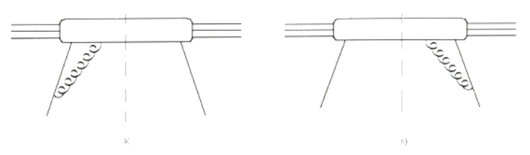
In particular, the interference term is such that the gluons (for ) are attached to the left quark leg, see figs. 2a and 3a. An important result, deduced at the end of Appendix A, is that such a term turns out to correspond to any interference term between two amplitudes, such that and gluons respectively are exchanged between the active quark and the spectator partons, with . The situation is illustrated in figs. 2 and 3 for = 1 and 2.

It is worth noting that a radiation ordering similar to the one established here is found in semiinclusive processes at large (Catani et al., 1991a) and in totally inclusive DIS at small (Catani et al., 1991b). Moreover the terms (22) consist of quark-gluon-quark correlations, analogous to the one introduced by Efremov and Teryaev (1984) and by Qiu and Sterman (1991, 1992, 1998).
As a consequence of the Politzer theorem, formulae (15) to (22) hold for renormalized fields, provided we take into account the scale dependence of the coupling , of the quark mass and of the correlators (Rogers, 2007). Moreover one has to observe that the four-momenta appearing in the propagators are highly off-shell: and are of order (Collins and Soper, 1982; Levelt and Mulders, 1994), because the uncertainty principle demands hard interactions to occur in a very limited space-time interval, corresponding to the condition
| (28) |
Therefore we have and , whence
| (29) |
and it follows that the coefficients are of order , up to QCD corrections, consisting of terms of the type , with and integers and (Dokshitzer et al., 1980). For the same reason, the coupling , which appears in expansion (15), assumes small values, corresponding to short distances and times.
To summarize, we have found that the T-even and the T-odd correlators, given by eqs. (7), may be written as expansions in , i. e.,
| (30) |
where has a relatively weak -dependence, as told above. Moreover, as already explained, changes sign when involved in DY. Stated differently, T-odd terms present an odd number of quark propagators, see eq. (20) for odd : in the limit of negligible quark mass, quark four-momenta in DIS are spacelike, whereas in DY they are timelike (Boer et al., 2003b).
The first two terms of expansion (15) will be studied in detail in sects. 4 and 5 respectively.
3 Hadronic Tensor
In the present section we refer indifferently to the hadronic tensor of one of the three processes introduced. To be precise, among these, only DY involves two correlators of the type illustrated in the last section, whereas SIDIS and annihilation include respectively one and two fragmentation correlators. However, as we shall see in sect. 6, this object requires only minor modifications with respect to the correlator (5).
If we substitute this correlator into the hadronic tensor (1), this latter does not fulfil the requirement of electromagnetic gauge invariance: only the term of zero order in the coupling satisfies this condition. In order to get a complete gauge invariance at any order, we have to recall the interpretation given above of the correlator. For example, at first order in the coupling in SIDIS, we see that the ”hard” scattering amplitude - where we have denoted by and the initial and final quark and by a gluon - consists not only of the graph of fig. 4a, encoded in the first order term of the correlator, but also of the one represented in fig. 4b, which interferes coherently with it. This guarantees electromagnetic gauge invariance for the first order graph (Berger and Brodsky, 1979).

Furthermore, convoluting ”hard” graphs with the ”soft” factors, these two amplitudes give rise, among other objects, to asymmetric Feynman-Cutkosky graphs (fig. 5), related to interference terms. These are observables - necessarily gauge invariant - and therefore assume real values. This procedure, already suggested by LM, can be generalized to the three kinds of hadronic tensors considered in the present article, at any order in , so as to obtain sets of graphs corresponding to observable, and therefore gauge invariant, quantities. We show how to construct them at any order , corresponding to the overall number of gluons exchanged between active quarks and spectator partons. The procedure consists in the following steps, for a given :
- Consider the possible combinations of gluons occurring in the hadronic tensor (1), say, for hadron and for hadron , with = 0, 1 … .
- For a given , consider all possible correlators, according to the definition given in subsect. 2.2: as seen at the end of last section, these amount to correlators equal to .
- Add each such correlator all those graphs whose ”hard” parts interfere coherently with it, as shown in fig. 5. In practice, one has to do this for the correlator whose gluons are attached to the ”left” quark leg and to multiply by the number of gluons of each correlator.

Then we have, up to QCD corrections at each order of the expansion,
| (31) |
with
| (32) | |||||
| (33) | |||||
| (34) |
Here we have used the following shorthand notations:
| (35) |
and are defined analogously to eqs. (20) and (22): the matrix product starts from and from respectively, rather than from . In particular, coincides with the definition (20). Last, we have set = 1.
For each term of expansion (31) we have to take into account three kinds of effects:
a) gluon radiation by scattered partons;
b) perturbative QCD corrections;
c) higher correlators, such that the active quarks exchange gluons with quark-antiquark pairs or gluon pairs or triplets belonging to spectator partons.
The first two effects may be calculated according to the algorithm suggested by Collins and Soper (1981, 1982). As to the contributions c), they can be included in the basic term of expansion (31), since they have the same (T-even or T-odd) behavior. Lastly we recall that, unless we integrate over some final transverse momentum [of the lepton pair in the case of DY, of a final hadron in SIDIS or annihilation], the phase space of the final gluons emitted undergoes a restriction (Dokshitzer et al., 1980), expressed by a doubly logarithmic form factor; this is more and more sizable at increasing energy, resulting in the well-known Sudakov-like damping (Collins and Soper, 1981; Boer, 1999).
4 Zero order term: the QCD parton model
In this section and in the next one we elaborate the first two terms of the expansion of the hadronic tensor. To this end we define a suitable reference frame, such that the momentum of the hadron has an opposite direction to the momentum of the hadron , and are of order and the -axis is along . Moreover we focus on the hadronic tensor for DY process. However, as told at the beginning of the previous section, our results can be trivially extended to SIDIS and annihilation; the main difference, concerning the fragmentation function, will be discussed in sect. 6.
Let us consider the hadronic tensor (32) at zero order, i. e.,
| (36) |
Here the ’s are given by eq. (16), for = 0, and fulfil the homogeneous Dirac equation (17). Incidentally, they are T-even and gauge invariant at zero order in . Moreover is defined by eq. (2). The tensor (36), T-even itself, can be calculated, once we know the ”soft” functions involved in the parameterizations of the correlators ’s. We show in Appendix B that
| (37) |
Here , and are functions of the four-momentum of the active quark, which, in this case, is on shell: , with . and are the components of the quark PL vector, respectively parallel and perpendicular to the hadron momentum. Moreover we have set
| (38) |
having defined the dimensionless, light-like four-vectors in such a way that
| (39) |
and such that their spatial components are along (+) or opposite (-) to the hadron momentum. It is important to notice that, if integrated over , the expression obtained for the zero order correlator turns out to be proportional to the density matrix of a quark confined in a finite volume, but free of interactions with other partons (Di Salvo, 2007b). Therefore we fix the normalization constant so as to obtain, after integration, just the density matrix i. e.,
| (40) |
Lastly, it is convenient to express and in terms of the components of the PL vector of the hadron. As shown in Appendix B, one has
| (41) |
Here
| (42) | |||||
| (43) | |||||
| (44) |
and is the transverse momentum of the active quark with respect to the hadron momentum.
Equation (37) has important consequences on TMD T-even functions, as we are going to illustrate in the two next subsections. To this end we compare that equation with the naive parameterization of the TMD correlator in terms of Dirac components, without introducing any dynamic conditions (Mulders and Tangerman, 1996; Boer et al., 2000; Goeke et al., 2005). We give such a parameterization in Appendix C, up to and including twist-3 terms. The twist-2, T-even sector, which we study in subsect. 4.1, corresponds to quark distribution functions which survive when interactions with gluons are turned off. As regards the twist-3 functions, we distinguish among the T-even, the T-odd and the ”hybrid” ones, these lasts deriving contributions both from T-even and T-odd terms.
4.1 Twist-2, T-even Correlator
If quark-gluon interactions are neglected, the correlator includes just twist-2, T-even terms. We show in Appendix C that it can be parameterized as
| (45) | |||||
Here we have adopted the usual notations for the non-perturbative functions (Kotzinian, 1995; Tangerman and Mulders, 1995); the indices and of denote respectively the feature of ”free” and ”T-even”. The Dirac operators considered are purely T-even, as can be checked; moreover
| (46) |
and is an undetermined energy scale, introduced for dimensional reasons, in such a way that all functions embodied in the parameterization of have the dimensions of a probability density. This scale (Kotzinian, 1995) determines the normalization of the functions which depend on . In particular, as is well-known, the 6 twist-2 functions, which appear in the parameterization (45), are interpreted as TMD probability densities: is the unpolarized quark density, the longitudinally polarized density in a longitudinally polarized (spin 1/2) hadron, the longitudinally polarized density in a transversely polarized hadron, the transversity in a longitudinally polarized hadron and
| (47) |
is the TMD transversity in a transversely polarized hadron§§ § The function is known as ”pretzelosity” (Avakian et al., 2008b)..
Now we compare the parameterization (45) with the correlator (37). To this end we consider projections of both matrices over the various Dirac components, i. e., for a given Dirac operator ,
| (48) |
taking into account eqs. (41) wherever necessary.
First of all, = and ( = 1, 2) yield, approximately in the limit of = 0,
| (49) |
These relations hold up to terms of order , since, as we have seen, the T-even Dirac components of derive contributions only from even powers of . Moreover, the Politzer theorem implies that the relations are not modified by renormalization effects, and therefore hold also taking into account QCD evolution.
In order to determine , we observe that the functions involved in both sides of eqs. (49) are independent of . Therefore we must set , being a dimensionless numerical constant, independent of momentum. But since these functions are quark densities, they should be normalized adequately, setting = 1. Then, neglecting the quark mass,
| (50) |
This result differs from the treatments of previous authors (Mulders and Tangerman, 1996; Goeke et al., 2005), who assume . Some mismatches have been shown, as consequences of this choice (Bacchetta et al., 2008); these could be eliminated by taking into account result (50).
4.2 Twist-3, ”Hybrid” Correlator
Now we consider a sector of the correlator which, as explained above in this section, has both T-even and T-odd contributions. In particular, here we focus on that part of ”hybrid” correlator which comes from the so-called ”kinematic” twist-3 terms. In Appendix C we find, according to the usual notations (Mulders and Tangerman, 1996; Goeke et al., 2005),
| (51) | |||||
Comparing the operator (51) with the correlator (37), and considering, in particular, the projections of over = ( = 1, 2) of such operators, yields the approximate relation
| (52) |
which corresponds to the Cahn (1978, 1989) effect and is approximately verified for sufficiently large and small (Anselmino et al., 2007). Also this equation, like eqs. (49), survives QCD evolution. As we shall see in the next section, eq. (52) holds up to terms of order , since derives also T-odd contributions from one-gluon exchange.
The projections of the same operators over = ( = 1, 2) yield (after integration over )
| (53) |
Here
| (54) |
and
| (55) |
This last equation has been obtained from eq. (47). The contribution of the QCD parton model to is very small: is negligible for - and -quarks, while for -quarks is presumably small, because the sea is produced mainly by annihilation of gluons, whose transversity is zero in a nucleon. Therefore the contribution of quark-gluon interactions, neglected in the approximation considered, becomes prevalent in this case, as well as for = and , corresponding respectively to the functions and in eq. (51). The effect of such interactions will be discussed in sect. 5.
4.3 Remarks
To conclude this section, we sketch some consequences of our theoretical results.
A) In the expression (47) or (55) for transversity, the second term is due to a relativistic effect. To illustrate this, consider a transversely polarized hadron. The longitudinal polarization of the quark, due in this case to the transverse momentum, is magnified by the boost from the quark rest frame. This additional polarization, along the quark momentum, has again a transverse component with respect to the nucleon momentum.
B) Eq. (55), together with the last two eqs. (49), suggests a method for determining approximately the nucleon transversity. Indeed, can be conveniently extracted from double spin asymmetry (Kotzinian and Mulders, 1996; Di Salvo, 2002, 2003) in SIDIS with a transversely polarized target. This asymmetry is expressed as a convolution of the unknown function with the usual, well-known fragmentation function of the pion. Therefore the method appears complementary to the one usually proposed (Airapetian et al., 2000; Anselmino et al., 2007), based on the Collins (1993) effect in single spin SIDIS asymmetry; in this latter case one is faced with the convolutive product of with the Collins function, which is poorly known (Efremov et al., 2006a,b).
C) Eq. (53) establishes a relation between transversity and transverse spin. Indeed, the two quantities are related to each other. But, unlike transversity, the transverse spin operator is chiral even and does not commute with the free hamiltonian of a quark (Jaffe and Ji, 1991a): in QCD parton model it is proportional to the quark rest mass, which causes chirality flip.
D) We note that , and are associated with ”twist-2” Dirac operators (Jaffe and Ji, 1991a, 1992), and yet, in our treatment, they are multiplied by inverse powers of , as results from eqs. (45) and (50): for the first two functions, for the third one. This would be unacceptable for common distribution functions; but, when transverse momentum is involved, also the orbital angular momentum plays a role. To illustrate this point, we recall that the quark distribution functions may be regarded as the absorptive parts of -channel quark-hadron amplitudes (Soffer, 1995). For example, corresponds to an amplitude of the type , denoting by a state in which the nucleon and quark helicities are, respectively, and . The amplitudes corresponding to the functions in question involve a change (for and ) or (for ) in the orbital angular momentum; therefore they are of the type
| (56) |
where = is the angle between the nucleon momentum and the quark momentum, while is weakly energy dependent. But is of order and of order . Therefore eq. (56) reproduces the -dependence of the coefficients relative to the above mentioned functions¶¶ ¶ This observation is the fruit of a stimulating discussion with Nello Paver..
5 First Order Correction
The first order correction in of the hadronic tensor reads [see eqs. (32) and (33)]
| (57) |
Here we have set
| (58) |
and
| (59) |
Furthermore the ’s are given by eq. (22) for = 1 and fulfil the homogeneous Dirac equation
| (60) |
Therefore, in the gauge adopted, this function is parameterized as
| (61) |
Here we have set
| (62) |
and
| (63) |
This is a consequence of the Politzer theorem, as shown in Appendix B. The quantities , , and are correlation functions of and . In particular, we have (see subsect. B.2)
| (64) | |||||
| (65) | |||||
| (66) | |||||
| (67) |
Here the ( = 1,2,3) are unpolarized. () is a longitudinally (transversely) polarized function in a longitudinally (transversely) polarized nucleon. is a transversely polarized correlation function in an unpolarized nucleon: it is connected to quark-gluon interaction, for example, to a spin-orbit coupling (Brodsky et al., 2002a,b, 2003).
5.1 Approximate Factorization
The second term of eq. (59) is not factorizable, in agreement with the observations of various authors (Brodsky et al., 2002a,b, 2003; Peigné, 2002; Collins and Qiu, 2007), who have shown failures of universality (Peigné, 2002; Collins and Qiu, 2007) at large tranverse momentum. However, for sufficiently large , and adopting an axial gauge, this term is negligibly small (Berger and Brodsky, 1979) in comparison with the first one, which instead is factorizable. In fact, the gluon corresponding to the first term has a smaller offshellness than the one involved in the second term. This approximation is especially acceptable, even for relatively small , provided we limit ourselves to small transverse momenta (Collins, 2002) of the initial hadrons with respect to the direction of the momentum of the virtual photon in the center of mass of the DY pair. However, as already explained in sect. 2, also in the case when factorization is approximately satisfied, the T-odd distribution functions change sign from SIDIS to DY. We shall illustrate phenomenological implications of this change of sign in sect. 7.
In this approximation the tensor (57) amounts to
| (70) |
where
| (71) |
and is given by eq. (37). Then the tensor assumes a form similar to , giving rise to an approximate (Brodsky et al., 2002a) factorization of T-odd functions. Our conclusion is quite analogous to the one drawn by Collins (2002) and presents some similarity with the Qiu-Sterman (1991) assumption about the quark-gluon-quark correlation functions. In particular, as regards the factors , defined by eq. (71), we have to take into account eqs. (61) to (67), together with eqs. (41). These induce for the following parameterization, at twist-3 approximation:
| (72) | |||||
Here we have defined
| (73) | |||||
| (74) |
Moreover
| (75) | |||||
| (76) |
Lastly is defined by eqs. (62) and
| (77) |
The notations for the functions are somewhat similar to those introduced by Mulders and Tangerman (1996) and Goeke et al. (2005). The suffix in , , and denotes T-odd contribution to these three functions. They have T-even counterparts, as explained in sect. 4, eq. (51), where we introduced ”hybrid” functions. The T-odd functions are normalized coherently with their T-even counterparts, as can be seen from the factor in front of , eq. (72): indeed, considering the case of an approximately on-shell quark, we have
| (78) |
Furthermore the -factor in (78) is compensated by the factor present in the term with in expansion (15), but absent in the term with ; therefore also the phase of the T-odd functions is in agreement with the one of the T-even counterparts. It follows from such observations that the factor (78) in expression (72) automatically fixes also the normalization and the phase of the remaining functions included in .
Last, as already noticed in connection with correlation functions, the function describes a quark transverse polarization induced by quark-gluon interactions: this polarization, present also in spinless or unpolarized hadrons, is somewhat similar to the Boer-Mulders (1998) function, although it is twist-3 and not twist-2.
5.2 Twist-3, T-odd correlator
As explained in the previous subsection, , eq. (72), yields, in the approximation discussed above, the contribution to the quark correlator of quark-gluon interactions, at approximation. We compare this expression with the purely kinematic parameterization of the twist-3, interaction dependent correlator, as given in appendix C. In this way we obtain several approximate relations among the ”soft” functions involved in that parameterization. This last reads
| (79) |
Here is obtained from eq. (51), by substituting by , according to the rule just stated at the end of subsect. 5.1. On the other hand, from Appendix C we get
| (80) | |||||
Comparison between parameterization (79) and result (72), component by component, yields the following approximate relations:
| (81) | |||||
| (82) | |||||
| (83) | |||||
| (84) |
Also these equations survive QCD evolution, like eqs. (49) and (52). Aside from that, it is important to notice that the second eq. (81) implies, together with the second eq. (73) and with the third eq. (74),
a) that = 0;
b) that includes 5 independent functions in all.
5.3 Remarks
A) Some of the functions, which appear in the equalities (81) to (83), are longitudinally (, ) or transversely (, ) polarized in an unpolarized nucleon. Conversely, other functions are unpolarized in a longitudinally () or transversely ( and the ””-functions) polarized nucleon∥∥ ∥ is known as the Sivers (1990, 1991) function. This is a consequence of the spin-orbit coupling (Brodsky et al., 2002a) in gluon-quark interactions. Furthermore, unlike previous authors (Boer and Mulders, 1998; Boer et al., 2000; Goeke et al., 2005), we find that such functions are are associated to the same inverse power of , independent of the kind of polarization (longitudinal or transverse) of the quark or of the nucleon.
B) Among eqs. (81) to (84), those which concern only T-odd functions hold up to terms of order . On the contrary, those which involve ”hybrid” functions - including eq. (52) - hold up to terms of order . Analogous approximate relations of this latter type have been found by Avakian et al. (2008a) and by Efremov et al. (2009).
C) By integrating the correlator (72) over the transverse momentum of the quark, we obtain interesting results as regards twist-3 common functions. First of all, the fourth eq. (84) implies that derives just T-even contributions, and therefore, apart from the (negligible) term illustrated in the previous section, it is essentially of order . On the contrary, the main contributions to and are of order and are T-odd; therefore they change sign according as to whether they are involved in DIS or DY reaction. These last predictions could be tested by confronting the DIS double spin asymmetry (Anthony et al., 1996a,b, 2003) with the DY one (Di Salvo, 2001; Soffer and Taxil, 1980). In the case of DY one has to integrate over the transverse momentum of the virtual photon; moreover, if possible, it may be more promising to detect pairs, whose polarization is perhaps less problematic to determine (Kodaira and Yokoya, 2003).
D) Lastly, the twist-2 T-odd functions , corresponding to transverse polarization in an unpolarized nucleon, and the unpolarized distribution function (Boer and Mulders, 1998) in a tranversely polarized nucleon find no place in parameterization (72).
5.4 Consequences on and
Now we examine some consequences of our results on the DIS structure functions and , whose properties have been studied by various authors (Anselmino et al., 1995; Jaffe and Ji, 1991b; Bluemlein and Tkablaze, 1999). To this end, here, and only in this subsection, we re-introduce the flavor indices, dropped out in formula (1), in order to recover the usual definitions of those functions. Moreover, we recall that
| (85) |
where is the fractional charge of the flavour and the barred quantities refer to antiquarks. On the other hand,
| (86) |
Here we have defined
| (87) |
But eq. (53) implies
| (88) |
As discussed in subsect. 4.2, is negligibly small for a nucleon. Therefore our result is in contrast with the Burkhardt-Cottigham (1970) (BC) sum rule, i. e.,
| (89) |
Indeed, integrating both sides of eq. (86) between 0 and 1, and assuming relation (89), implies
| (90) |
But this result is unacceptable, since a twist-2, T-even function like has a priori no relation with , which is twist-3 and T-odd.
Furthermore eq. (89) implies, together with the operator product expansion (Anselmino et al., 1995),
| (91) |
where is the twist-3 contribution to (Anselmino et al., 1995), to be identified, according to our results, with . Then eq. (86) would yield
| (92) |
which appears in contrast with data of (Ashman et al., 1988, 1989; Airapetian et al., 1998), enforcing arguments against the BC rule (See Anselmino et al. (1995) and articles cited therein). An experimental confirmation of the violation of the BC rule was found years ago in a precision measurement of (Anthony et al., 2003).
Also the Efremov-Leader-Teryaev (ELT) sum rule, according to the version given by Anselmino et al. (1995), i. e.,
| (93) |
is in contrast with our result. Indeed, it gives rise, together with eqs. (86) and (88), to the approximate relation
| (94) |
which, again, relates a T-even function to a T-odd one. However, it is worth noting that the ELT sum rule was successively reformulated (Efremov et al., 1997) by suitably redefining and .
6 Fragmentation Correlator
The fragmentation correlator (4) can be made gauge invariant analogously to the distribution correlator, i. e., for a quark,
| (95) |
where is given by eq. (6). The object (95) may be treated analogously to the distribution correlator, according to the previous sections. Indeed, also in this case, for an antiquark one has to change the four-momentum from to and to put a minus sign in front of the correlator. Moreover one has to choose the path for quark fragmentation from annihilation, whereas the path refers to fragmentation in SIDIS. The only important difference with the distribution correlator is that one has to take into account also the nonperturbative interactions among the final hadrons produced. However, as we shall see in a moment, this does not involve any change in the parameterization.
We treat only the case of pions, adopting for T-odd terms an approximation analogous to the one discussed in subsection 5.1, valid for small transverse momenta of the final hadron with respect to the fragmenting quark. Under this condition, we have
| (96) | |||||
| (97) | |||||
| (98) |
Here is the common fragmentation function of the pion; , defined according to Mulders and Tangerman (1996), is the analog of ; last, assumes the role of the Collins (1993) function, describing the asymmetry of a pion fragmented from a transversely polarized quark, the so-called Collins asymmetry (see also Leader, 2004).
Final state interactions give rise to terms which decrease as inverse powers of , independent of the nature of the interactions themselves. As an example, we re-consider the interactions which produce the above mentioned Collins asymmetry from a different point of view. Analogously to the distribution functions illustrated in remark D at subsect. 4.3, such an asymmetry may be connected to the absorptive part of an amplitude of the type , where denotes the helicity of the fragmenting quark. This kind of amplitude - a typical helicity flip one - behaves as
| (99) |
where is a given function, weakly dependent on the quark momentum. Then, similarly to eq. (56), we conclude that the effect of the final state interaction between the fragmenting quark and the fragmented hadron decreases like . This confirms our previous result, but independent of the nature of the interaction.
More generally, we examine the interactions that the fragmented hadron, say hadron , undergoes with other final hadrons. These cause in the momentum of a change which depends weakly on , since the multiplicity of the hadrons produced in inclusive reactions increases only logarithmically with energy. Moreover, for sufficiently large and not too small fractional momenta of with respect to the fragmenting quark, the ratio
| (100) |
is quite small. Then, under such conditions, decreases approximately like . Our result agrees with the approach by Collins and Soper (1981), who do not include ”soft” final state interaction in the leading term of (almost) back-to-back fragmentation in annihilation.
7 Asymmetries
In this section we consider some important azimuthal and single spin asymmetries, which, as is well known, may be produced by coupling two chiral-even or two chiral-odd TMD distribution or fragmentation functions. More precisely, the terms of the hadronic tensor which give rise to asymmetries are written as convolutive products of two ”soft” functions times a suitable weight function (Boer et al., 2000; Di Salvo, 2007a) which changes from asymmetry to asymmetry. These last depend on some azimuthal angle , relative to the final hadron (for SIDIS and annihilation), or to the final muon pair (for DY). Some of these asymmetries arise from the first order correction of the hadronic tensor, while others belong to the second order one, whose complete parameterization is not considered in this paper.
A) Cahn effect
This effect, pointed out for the first time by Cahn (1978), has been exhibited by Anselmino et al. (2007) examining some SIDIS data (Arneodo et al., 1987; Ashman et al., 1991; Adams et al., 1993) (see also Anselmino et al., 2006). We consider the asymmetry corresponding to the ”product”
| (101) |
This asymmetry is proportional to and decreases like . To the extent that and can be approximated by and respectively, one speaks properly of Cahn effect (Anselmino et al., 2007): this amounts to neglecting quark-gluon interactions, see eq. (52) for distribution functions, an analogous equation holding for unpolarized fragmentation functions. This approximation is acceptable for relatively large and at small , as shown by Anselmino et al. (2007). However, one has to observe that both and are ”hybrid” functions and in general their T-odd contributions cannot be neglected.
It is worth considering also the ”product”
| (102) |
which generates a asymmetry decreasing like , hardly distinguishable from another one, arising from the ”product” of two chiral-odd functions, as we shall see in a moment. Under the approximation just discussed, we predict a sort of ”second order” Cahn effect.
B) Qiu-Sterman effect
An important transverse single spin asymmetry is the one predicted by Qiu and Sterman (1991, 1992, 1998) (QS) (see also Efremov and Teryaev, 1984, 1985; Boer et al., 1998, 2003b). This can be observed both in SIDIS and in DY, by integrating over the transverse momentum of the final hadron detected (SIDIS) or of the final pair (DY). This is described by the ”products”
| (103) |
the ”bar” indicating the antiquark function and ”charge conjugated”. A similar effect could be observed in annihilation, if one of the final hadrons observed is spinning. This asymmetry decreases like . Moreover, since is prevalently T-odd, while , and are T-even, the asymmetry is expected to assume an opposite sign in SIDIS and DY.
C) Sivers effect
The Sivers (1990, 1991) single transverse spin asymmetry is described by the ”product”
| (104) |
This asymmetry was detected by HERMES (Airapetian et al., 2005b; Diefenthaler, 2005) and COMPASS (Alexakhin et al., 2005) experiments. It is T-odd, since it consists of the ”product” of a T-odd function () times a T-even function ( or ). Therefore the asymmetry is predicted to change sign (Collins, 2002; Collins et al., 2006; Anselmino et al., 2009), according as to whether it is observed in SIDIS or DY, similar to the QS effect.
However the T-odd character of leads us to conclude that the Sivers asymmetry decreases like , in disagreement with the current literature (Boer and Mulders, 1998; Efremov et al., 2006b; Anselmino et al., 2007).
Furthermore the third eq. (81), i. e., , implies, together with eqs. (103) and (104), that the Sivers and QS asymmetries are related to each other, although the weight functions (Boer et al., 2000; Di Salvo, 2007a) involved in the two ”products” are different. This analogy was already noticed by other authors (Boer et al., 2003b; Ji et al., 2006a,b,c; Koike et al., 2008).
D) Collins effect and Boer-Mulders effect
In the framework of chiral-odd functions, an important single spin asymmetry is produced by combination of two transversities. In particular, single transverse polarization gives rise to an asymmetry described by the ”product”
| (105) | |||||
| (106) |
The asymmetry - predicted by Collins (1993) and exhibited by HERMES data (Airapetian et al., 2005b; Diefenthaler, 2005) - decreases like according to our treatment. It has been studied recently by Leader (2004), Anselmino (2009, 2010) and Boer (2009).
We have also the following azimuthal, asymmetries:
| (107) | |||||
| (108) | |||||
| (109) |
which decrease like . Therefore, as in the case of the Sivers asymmetry, we obtain a dependence of asymmetries (105) to (109) which differs from other authors (Boer and Mulders, 1998; Efremov et al., 2006a; Burkardt and Hannafious, 2008). Our prediction for the Boer-Mulders asymmetry is supported (Di Salvo, 2007a) by DY data (Falciano et al., 1986; Guanziroli et al., 1988; Conway et al., 1989). On the other hand, the dependence of the Collins and Sivers asymmetries might be tested in new planned experiments at higher energies (Afanasev et al., Jefferson Lab., hep-ph/0703288, 2007).
8 Summary
In the present paper we have studied the gauge invariant quark-quark correlator, which we have expanded in powers of the coupling and split into a T-even and a T-odd part. Working in the KS gauge, the Politzer theorem on EOM has allowed us to interpret each term of the expansion according to Feynman-Cutkosky graphs, involving higher correlators and corresponding to powers of . We have also elaborated an algorithm for writing a gauge invariant sector of the hadronic tensor in deep inelastic processes, like SIDIS, DY and annihilation. This gives rise to a rather long and complicated sum of terms. However, in the gauge considered, and especially at small transverse momenta, the ”Born” terms of the type (1) prevail over the remaining ones, as we have shown explicitly for first order correction in .
The zero order term and the first order correction of the expansion have been examined in detail. In both cases the Politzer theorem produces a considerable reduction of independent functions with respect to the naive parameterization in terms of Dirac components, giving rise to approximate (up to powers of ) relations among ”soft” functions. These relations survive QCD evolution. One such relation has been approximately verified against experimental data (Airapetian et al., 2005b; Avakian et al., 2005), another one suggests a method for determining approximately transversity, while others could be checked in next experiments (Bunce et al., 2000; Adams et al., 1993). Also an energy scale, introduced in the naive parameterization for dimensional reasons, has been determined in our approach, leading to predictions on dependence of various azimuthal asymmetries. One of these predictions finds confirmation in unpolarized DY data (Falciano et al., 1986; Guanziroli et al., 1988; Conway et al., 1989). The hierarchy of TMD functions in terms of inverse powers of is established taking into account not only the Dirac operators, as in the case of common functions (Jaffe and Ji, 1991a, 1992), but also the dependence, since in this case the orbital angular momentum plays a role as well as spin.
Moreover a relation is found among , the QS asymmetry and the Sivers asymmetry; in particular, both and the two asymmetries are found to change sign according as to whether they are observed in SIDIS or in DY. We draw also some conclusions about the structure function , in particular against the BC sum rule.
Quark fragmentation involves ”soft” interactions among final hadrons, but this does not imply a substantial difference with the distribution correlator. Rather, a caveat should be kept in mind for timelike photons, in DY and annihilation, when approaches the energy of a vector boson resonance, like the or the . Since such a resonance interferes with the photon, one has to take into account its offshellness, quite different than . A particular attention has to be paid also to the case when the active quark (or antiquark) comes from gluon annihilation, as occurs, for example, in DY from proton-proton collisions. This may give rise to T-odd Feynman-Cutkosky graphs, in which the (anti-)quark propagator is only slightly off-shell. These two situations deserve a separate treatment.
As a conclusion, we stress that, although other authors, like EFP, LT and Efremov and Teryaev (1984) already proposed, years ago, a decomposition of the hadronic tensor in terms of Feynman-Cutkosky graphs, our deduction, based on EOM, leads to strong constraints on the parameterization of the ”soft” parts of the graphs.
Acknowledgments
The author is grateful to his friends A. Blasi, A. Di Giacomo and N. Paver for fruitful discussions.
Appendix A
We deduce a recursion formula for the terms of the expansion of the correlator. Our starting point is the Politzer (1980) theorem, which implies
| (A. 1) |
Here denotes the state of a hadron (for instance, but not necessarily, a nucleon) with four-momentum and PL four-vector . is the quark field, of which we omit the color and flavor index. is the covariant derivative, adopting for the gluon field the shorthand notation for . For the sake of simplicity, color and flavor indices of the quark field have been omitted. Moreover
| (A. 2) |
where is the strong coupling, while . We have, for , in the KS gauge,
| (A. 3) |
Here we have adopted the reference frame and the notations and definitions introduced in sect. 2. In particular, is related to : , . It is worth observing that
| (A. 4) |
Substituting expansion (A. 2) into eq. (A. 1), we get
| (A. 5) |
with
| (A. 6) |
Eq. (A. 5) is an operator equation, to be intended in a weak sense: it holds when calculated between hadronic states. All equations of this Appendix will be of this type from now on.
Looking for a perturbative solution for the correlator in powers of , we set each term of the series (A. 5) equal to zero, i. e.,
| (A. 7) |
where
| (A. 8) |
By Fourier transforming both sides of eq. (A. 7), and recalling relation (A. 4), we get
| (A. 9) |
where
| (A. 10) |
Eq. (A. 9) can be rewritten as
| (A. 11) |
where
| (A. 12) | |||||
| (A. 13) |
Eq. (A. 11) is a recursion formula for , eqs. (A. 6) constituting the first steps. This formula implies eqs. (17) (for = 0) and (18) (for ) in the text. In particular, as regards eq. (18), the quantity results in
| (A. 14) |
where is a normalization constant. The operator in eq. (A. 11) corresponds to a graph endowed with gluons, such that the -th gluon leg is attached to the quark leg on the left side of the graph (see figs. 2a and 3a).
Taking into account the hermitian character of and the relation , eq. (A. 11) implies
| (A. 15) |
In this case corresponds again to a graph with gluons, but such that the -th gluon is attached to the quark leg on the right side of the graph. This last result implies that represents any graph with gluons, each gluon leg being attached to the left or right quark leg.
Appendix B
Here we deduce the parameterizations of the quark-quark correlator at zero order and of the quark-gluon-quark correlation, arising from first order correction.
B.1. The Zero Order Quark-Quark Correlator
The matrix , defined by
| (B. 1) |
fulfils the homogeneous Dirac equation
| (B. 2) |
where is the rest mass of the quark. As shown in Appendix A, this is a consequence of the Politzer theorem. This implies, at zero order in the coupling,
| (B. 3) |
Therefore, in the approximation considered, the quark can be treated as if it were on shell (see also Qiu, 1990). Then, initially, we consider the Fourier expansion of the unrenormalized field of an on-shell quark, i. e.,
| (B. 4) |
Here is the spin component of the quark along a given direction in the quark rest frame, its four-spinor, the destruction operator for the flavor considered and
| (B. 5) |
As regards the normalization of and , we assume
| (B. 6) |
where
| (B. 7) |
and is the probability density to find a quark with spin component and four-momentum , with . For an antiquark the definition is analogous, except that, in the Fourier expansion (B. 4), we have to substitute the destruction operators with the creation operators and with in the exponential.
Choosing the quantization axis along the hadron momentum in the frame defined at the beginning of sect. 4, and substituting eq. (B. 4) into eq. (B. 1), we get
| (B. 8) | |||||
But owing to the second eq. (B. 6) we have
| (B. 9) |
where
| (B. 10) | |||||
| (B. 11) |
Firstly we elaborate . We have
| (B. 12) |
Here is a four-vector such that, in the quark rest frame, , , and is the unit spin vector of the hadron in its rest frame. Therefore
| (B. 13) |
where
| (B. 14) |
is the unpolarized transverse momentum distribution of the quark, while
| (B. 15) |
According to transformation properties of one-particle states under rotations, one has
| (B. 16) |
where denotes the (positive or negative) helicity of the hadron and the angle between and . Substituting eq. (B. 16) into eq. (B. 15), and taking into account parity conservation, we get
| (B. 17) |
Here
| (B. 18) |
is the longitudinally polarized TMD distribution of the quark, the last equality following from parity conservation.
Now we consider . Eq. (B. 16) yields, for ,
| (B. 19) |
where and denote quark states with spin components, respectively, along and along
| (B. 20) |
Substituting eqs. (B. 16) and (B. 19) into eq. (B. 11), and taking into account again parity conservation, we get
| (B. 21) |
where
| (B. 22) |
is the TMD transversity of the quark. Returning to the Dirac notation, we have
| (B. 23) |
where is such that in the quark rest frame and
| (B. 24) |
Then eq. (B. 21) goes over into
| (B. 25) |
Substituting eqs. (B. 13), (B. 17) and (B. 25) into eq. (B. 9) yields
| (B. 26) |
having set and . Eq. (B. 26) is a solution to eq. (B. 2), which is a consequence of the Politzer theorem at zero order in . Since this equation survives renormalization - which generally implies only a weak -dependence (Sterman, 2005; Dokshitzer et al., 1980) - the structure of is not changed by QCD evolution.
Lastly we deduce the expressions of the four-vectors and in the frame where the quark momentum is . In the quark rest frame we have
| (B. 27) |
In view of the Lorentz boost, it is convenient to further decompose and into components parallel and perpendicular to the quark momentum. We have
| (B. 28) | |||||
| (B. 29) |
where
| (B. 30) | |||||
| (B. 31) |
The boost which transforms the four-momentum of the quark from to , with , changes only the components along of and of . In particular, the boost transforms the four-vector to , with . Therefore, since and are and , eqs. (B. 27) go over into
| (B. 32) |
where and .
B.2. The Quark-Gluon-Quark Correlator
Now we deduce a parameterization for the quark-gluon-quark correlator, defined by
| (B. 33) |
As shown in Appendix A, the Politzer theorem implies, at order 1 in the coupling,
| (B. 34) |
which holds also after renormalization. Therefore our line of reasoning is the same as for , that is, we start from unrenormalized fields and we take on-shell quarks, whose field satisfies expansion (B. 4). Substituting this expansion into eq. (B. 33), we get
| (B. 35) | |||||
| (B. 36) |
Here and are defined analogously to eqs. (B. 5),
| (B. 37) |
and
| (B. 38) |
Moreover the matrix element (B. 38) fulfils a relation of the type
| (B. 39) |
where is a quark-gluon correlator and , and are defined by eq. (B. 7). Then eq. (B. 36) yields
| (B. 40) |
and
| (B. 41) |
We rewrite eq. (B. 40) as
| (B. 42) |
where
| (B. 43) | |||||
| (B. 44) |
Taking into account the appropriate Lorentz transformations for the spinors involved, we have
| (B. 45) | |||||
| (B. 46) |
Here
| (B. 47) |
| (B. 48) | |||||
| (B. 49) |
analogous definitions holding for and . Moreover and refer to the PL vector of a quark with four-momentum , directly connected with nucleon polarization; they can be related to the nucleon longitudinal and transverse PL vectors, using the formulae elaborated at the end of sect. B1. refers to the spin caused by spin-orbit coupling,
| (B. 50) |
Last, is a real, ”soft” parameter, which in general will depend on and ; it will be included in the definitions of two of the ”soft” correlation functions.
We assume , where and are, respectively, the angle between and and the one between and . Then
| (B. 51) |
with
| (B. 52) | |||||
| (B. 53) |
Then results in
| (B. 54) |
where
| (B. 55) |
and
| (B. 56) | |||||
| (B. 57) | |||||
| (B. 58) | |||||
| (B. 59) |
are correlation functions. In order to parameterize these functions, we recall the definition (B. 33) of quark-gluon-quark correlator and eq. (9), concerning the gauge used. Therefore we have to take into account the available transverse four-vectors, whence it follows that
| (B. 60) | |||||
| (B. 61) | |||||
| (B. 62) | |||||
| (B. 63) |
Here , , , , and are ”soft” functions of and . The parameterization of is obtained by inserting eqs. (B. 54) and (B. 60) to (B. 63) into eq. (B. 35). Again, as in the case of , the Politzer theorem, of which eq. (B. 34) is a consequence, implies that renormalization effects preserve the structure of that parameterization.
Appendix C
Here we consider the parameterization of the correlator in terms of the Dirac components, up to and including twist-3 terms. This parameterization is similar to the usual ones (Boer and Mulders, 1998; Goeke et al., 2005), also as regards notations, except for an energy scale , which we leave undetermined here, and for the twist-2, T-odd sector, which we omit because it has no place in our procedure. The scale , usually set equal to the rest mass of the hadron, is determined in sects. 4 and 5, with a different result.
The parameterization reads
| (C. 1) |
Here
| (C. 2) | |||||
| (C. 3) | |||||
| (C. 4) | |||||
Here denotes the ”hybrid” term, both interaction free (, T-even) and interaction dependent (, T-odd): the two terms have the same parameterization, but behave quite differently. For the ”soft” functions we have adopted notations similar to those employed by Goeke et al. (2005). Note, however, that in the expression of the functions , , , and do not appear in the parameterization proposed by those authors; on the contrary, we have not taken into account the functions and , defined by them.
References
Abe, K., et al. (BELLE), 2006, Phys. Rev. Lett. 96, 232002
Abe, K., et al. (E143), 1998, Phys. Rev. D 58, 112003
Abe, K., et al. (E154), 1997a, Phys. Lett. B 405, 180
Abe, K., et al. (E154), 1997b, Phys. Rev. Lett. 79, 26
Adams, M.R., et al. (E665), 1993, Phys. Rev. D 48, 5057
Adeva, B., et al. (EMC), 1998, Phys. Rev. D 58, 112001
Ageev, E. S., et al. (COMPASS), 2007, Nucl. Phys B 765, 31
Airapetian, A., et al. (HERMES), 1998, Phys. Lett. B 442, 484
Airapetian, A., et al. (HERMES), 2000, Phys. Rev. Lett. 84, 4047
Airapetian, A., et al. (HERMES), 2001, Phys. Rev. D 64, 097101
Airapetian, A., et al. (HERMES), 2003, Phys. Lett. B 562, 182
Airapetian, A., et al. (HERMES), 2005a, Phys. Rev. Lett. 94, 012002
Airapetian, A., et al. (HERMES), 2005b, Phys. Rev. D 71, 012003
Alexakhin, V. Yu., et al. (COMPASS), 2005, Phys. Rev. Lett. 94, 202002
Alekseev, M. G., et al. (COMPASS), 2010a, Phys. Lett. B 692, 240
Alekseev, M. G., et al. (COMPASS), 2010b, Phys. Lett. B 693, 227
Anselmino, M., A. Efremov and E. Leader, 1995, Phys. Rep. 261, 1
Anselmino, M., A. Efremov, A. Kotzinian and B. Parsamyan, 2006, Phys. Rev. D 74, 074015
Anselmino, M., M. Boglione, U. D’Alesio, A. Kotzinian, F. Murgia, A. Prokudin and C. Turk, 2007, Phys. Rev. D 75, 054032
Anselmino, M., M. Boglione, U. D’Alesio, S. Melis, F. Murgia and A. Prokudin, 2009a, Phys. Rev. D 79, 054010
Anselmino, M., M. Boglione, U. D’Alesio, A. Kotzinian, S. Melis, F. Murgia, A. Prokudin and C. Turk, 2009b, Eur. Phys. Jou. A 39, 89
Anselmino, M., M. Boglione, U. D’Alesio, S. Melis, F. Murgia, and A. Prokudin, 2010, Phys. Rev. D 81, 034007
Anthony, P. L., et al. (E155), 2003, Phys. Lett. B 553, 18
Anthony, P. L., et al. (E142), 1996a, Phys. Rev. D 54, 6620
Anthony, P. L., et al. (E143), 1996b, Phys. Rev. Lett. 76, 587
Arneodo, M., et al. (EMC), 1987, Z. Phys. C 34, 277
Artru, X., and M. Mekhfi, 1990, Z. Phys. C 45, 669
Ashman, J., et al. (EMC), 1988, Phys. Lett. B 206, 364
Ashman, J., et al. (EMC), 1989, Nucl. Phys B 328, 1
Ashman, J., et al. (EMC), 1991, Z. Phys. C 52, 361
Avakian, H., P. Bosted, V. Burkert and L. Elouadrhiri, 2005, AIP Conf. Proc. 792, 945
Avakian, H., A. V. Efremov, K. Goeke, A. Metz, P. Schweitzer and T. Tecknentrup, 2008a, Phys. Rev. D 77, 014023
Avakian, H., A. V. Efremov, P. Schweitzer and F. Yuan, 2008b, Phys. Rev. D 78, 114024
Bacchetta, A., D. Boer, M. Diehl and P. J. Mulders, 2008, JHEP 0808:023
Belitsky, A. V., X. Ji and F. Yuan, 2003, Nucl. Phys. B 656, 165
Berger, E. L., and S. J. Brodsky, 1979, Phys. Rev. Lett. 42, 940
Bilal, A., et al., 1991, Nucl. Phys. B 355, 549
Bluemlein, J., and A. Tkabladze, 1999, Nucl. Phys. B 553, 427
Boer, D. and P. J. Mulders, 1998, Phys. Rev. D 57, 5780
Boer, D., P. J. Mulders and O. V. Teryaev, 1998, Phys. Rev. D 57, 3057
Boer, D., 1999, Phys. Rev. D 60, 014012
Boer, D., R. Jakob and P. J. Mulders, 2000, Nucl. Phys. B 564, 471
Boer, D., S. J. Brodsky and D.-S. Huang, 2003a, Phys. Rev. D 67, 054003
Boer, D., P. J. Mulders and F. Pijlman, 2003b, Nucl. Phys. B 667, 201
Boer, D., 2009, Nucl. Phys. B 806, 23
Boffi, S., A. V. Efremov, B. Pasquini and P. Schweitzer, 2009, Phys. Rev. D 79, 094012
Bomhof, C.J., P.J. Mulders and F. Pijlman, 2004, Phys. Lett. B 596, 277
Bravar, A. et al. (SMC), 1999, Nucl. Phys. B (Proc. Suppl.) 79, 520
Bressan, A. (COMPASS), 2007, Munich Deep inelastic scattering, Vol. , pag. 583
Brodsky, S. J., D. S. Hwang and I. Schmidt, 2002a, Phys. Lett. B 530, 99
Brodsky, S. J., D. S. Hwang and I. Schmidt, 2002b, Nucl. Phys. B 642, 344
Brodsky, S. J., D. S. Hwang and I. Schmidt, 2003, Int. Jou. Mod. Phys. A 18, 1327
Bunce, G., N. Saito, J. Soffer and W. Vogelsang, 2000, Ann. Rev. Nucl. Part. Sci. 50 525
Burkardt, M., and B. Hannafious, 2008, Phys. Lett. B 658, 130
Burkhardt, H., and W. N. Cottigham, 1970, Ann. Phys. 56, 453
Cahn, R.N., 1978, Phys. Lett. B 78, 269
Cahn, R.N., 1989, Phys. Rev. D 40, 3107
Catani, S., B. R. Webber and G. Marchesini, 1991a, Nucl. Phys. B 349, 635
Catani, S., B. R. Webber, F. Fiorani and G. Marchesini, 1991b, Nucl. Phys. B (Proc. Suppl.) 23, 123
Collins, J. C., 1993, Nucl. Phys. B 396, 161
Collins, J. C., A. V. Efremov, K. Goeke, M. Grosse Perdekamp, S. Menzel, B. Meredith, A. Metz and P. Schweitzer, 2006, Phys. Rev. D 73, 094023
Collins, J. C., 1998, Phys. Rev. D 57, 3051
Collins, J. C., 1989, Perturbative QCD, A.H. Mueller ed., World Scientific, Singapore
Collins, J. C., D. E. Soper and G. Sterman, 1988, Adv. Ser. Direct. High Energy Phys. 5, 1
Collins, J. C., and D. E. Soper, 1981, Nucl. Phys. B 193, 381
Collins, J. C., and D. E. Soper, 1982, Nucl. Phys. B 197, 446
Collins, J. C., 2002, Phys. Lett. B 536, 43
Collins, J. C., and J. Qiu, 2007, Phys. Rev. D 75, 114014
Conway, J.S., et al., 1989, Phys. Rev. D 39, 92
DeRujula, A., et al., 1971, Nucl. Phys. B 35, 365
Di Salvo, E., 2007a, Int. Jou. Mod. Phys. A 22, 2145
Di Salvo, E., 2007b, Mod. Phys. Lett. A 22, 1787
Di Salvo, E., 2003, Int. Jou. Mod. Phys. A 18, 5277
Di Salvo, E., 2002, Nucl. Phys. A 711, 76
Di Salvo, E., 2001, Eur. Phys. Jou. C 19, 503
Diefenthaler, M. (HERMES), 2005, AIP Conf. Proc. 792, 933
Dokshitzer, Yu. L., D. I. Dyakonov and S. I. Troyan, 1980, Phys. Rep. 58, 269
Ellis, R. K., W. Furmanski and R. Petronzio, 1982, Nucl. Phys. B 207, 1
Ellis, R. K., W. Furmanski and R. Petronzio, 1983, Nucl. Phys. B 212, 29
Efremov, A., and A. Radyushkin, 1981, Theoretical and Mathematical Physics 44, 774
Efremov, A., and O. Teryaev, 1984, Yad. Fiz. 39, 1517
Efremov, A. V., K. Goeke and P. Schweitzer, 2006a, Phys. Rev. D 73, 094025
Efremov, A. V., K. Goeke and P. Schweitzer, 2006b, Czech. J. Phys. 56, F181
Efremov, A. V., and O. Teryaev, 1985, Phys. Lett. B 150, 383
Efremov, A. V., P. Schweitzer, O. V. Teryaev and P. Zavada, 2009, Phys. Rev. D 80, 014021
Efremov, A. V., O. V. Teryaev and E. Leader, 1997 Phys. Rev. D 55, 4307
Falciano, S., et al. (NA10), 1986, Z. Phys. C - Particles and Fields 31, 513
Goeke, K., A. Metz and M. Schlegel, 2005, Phys. Lett. B 618, 90
Guanziroli, M., et al. (NA10), 1988, Z. Phys. C - Particles and Fields 37, 545
Hawranek, P. (PANDA), 2007, Int. Jou. Mod. Phys. A 22, 574
Jaffe, R. L., and X. Ji, 1991a, Phys. Rev. Lett. 67, 552
Jaffe, R. L., and X. Ji, 1991b, Phys. Rev. D 43, 724
Jaffe, R. L., and X. Ji, 1992, Nucl. Phys. B 375, 527
Ji, X., and F. Yuan, 2002, Phys. Lett. B 543, 66
Ji, X., J. W. Qiu, W. Vogelsang and F. Yuan, 2006a, Phys. Rev. Lett. 97, 082002
Ji, X., J. W. Qiu, W. Vogelsang and F. Yuan, 2006b, Phys. Rev. D 73, 094017
Ji, X., J. W. Qiu, W. Vogelsang and F. Yuan, 2006c, Phys. Lett. B 638, 178
Kodaira, J., and H. Yokoya, 2003, Phys. Rev. D 67, 074008
Kogut, J. B., and D. E. Soper, 1970, Phys. Rev. D 1, 2901
Koike, Y., W. Vogelsang and F. Yuan, 2008, Phys. Lett. B 659, 878
Kotzinian, A. M., 1995, Nucl. Phys. B 441, 234
Kotzinian, A. M., and P. J. Mulders, 1996, Phys. Rev. D 54, 1229
Lenisa, P. (PAX), 2005, AIP Conf. Proc. 792, 1023
Levelt, J., and P. J. Mulders, 1994, Phys. Rev. D 49, 96
Leader, E., 2004, Phys. Rev. D 70, 054019
McGaughey, P. L., et al. (E772), 1994, Phys. Rev. D 50, 3038
Mulders, P. J., and R. D. Tangerman, 1996, Nucl. Phys. B 461, 197
Peigné, S., 2002, Phys. Rev. D 66, 114011
Politzer, H. D., 1980, Nucl. Phys. B 172, 349
Qiu, J., and G. Sterman, 1991, Phys. Rev. Lett. 67, 2264
Qiu, J., and G. Sterman, 1992, Nucl. Phys. B 378, 52
Qiu, J., and G. Sterman, 1998, Phys. Rev. D 59, 014004
Qiu, J., 1990, Phys. Rev. D 42, 30
Ralston, J., and D. E. Soper, 1979, Nucl. Phys B 152, 109
Rogers, T. C., 2007, 8th International Symposium on Radiative Corrections (RADCOR), October 1-5, arXiv:hep-ph/0712.1195. See also references therein.
Sivers, D. W., 1990, Phys. Rev. D 41, 83
Sivers, D. W., 1991, Phys. Rev. D 43, 261
Sivers, D., 2006, Phys. Rev. D 74, 094008
Soffer, J., and P. Taxil, 1980, Nucl. Phys. B 172, 106
Soffer, J., 1995, Phys. Rev. Lett. 74, 1292
Sterman, G., 2005, Contribution to Elsevier Encyclopedia of Mathematical Physics, YITP-SB-05-27, hep-ph/0512344
Tangerman, R. D., and P. J. Mulders, 1995, Phys. Rev. D 51, 3357
Towell, R. S., et al. (E866), 2001, Phys. Rev. D 64, 052002
Yun, J., et al. (CLAS), 2003, Phys. Rev. C 67, 055204
Zheng, X., et al. (E-99-117), 2004, Phys. Rev. C 70, 065207
Zhu, L. Y., et al. (E866), 2007, Phys. Rev. Lett. 99, 082301