A Holographic Superconductor in an External Magnetic Field
Abstract:
We study a system of a complex charged scalar coupled to a Reissner–Nordström black hole in 3+1 dimensional anti–de Sitter spacetime, neglecting back–reaction. With suitable boundary conditions, the cases of a neutral and purely electric black hole have been studied in various limits and were shown to yield key elements of superconductivity in the dual 2+1 dimensional field theory, forming a condensate below a critical temperature. By adding magnetic charge to the black hole, we immerse the superconductor into an external magnetic field. We show that a family of condensates can form and we examine their structure. For finite magnetic field, they are localized in one dimension with a profile that is exactly solvable, since it maps to the quantum harmonic oscillator. As the magnetic field increases, the condensate shrinks in size, which is reminiscent of the Meissner effect.
Keywords:
AdS-CFT Correspondence, Gauge-gravity correspondence1 Introduction
Since the early days of AdS/CFT[1, 2, 3] (see ref. [4] for a review) it has been tempting to consider applying holographic duality to the study of important strongly coupled phenomena in condensed matter systems, and superconductivty has been high on the list11 1 The fact that certain black holes and branes are known to exhibit a sort of Meissner effect[5, 6, 7] at zero temperature has always added to the motivation, although it has not been clear how exactly this could be connected to a dual superconductivity.. Since finite temperature in these duals typically implies the presence of a black hole, and since superconductivity requires a condensate to form below a certain critical temperature, the existence of a holographically dual background would seem to require a circumvention of various statements of no–hair theorems (which go back to Wheeler[8] — for a review, see ref.[9]). Generically, the black holes would need to have some kind of scalar hair in order to be dual to a superconductor (the scalar’s asymptotic value would be the condensate vacuum expectation value (vev)).
In a series of studies[10, 11, 12], Gubser has presented a case for just the right kind of no–scalar–hair theorem evasion to allow for a superconductor’s dual to exist. The statement seems to be that there do exist solutions that allow for a condensing scalar to be coupled to the black hole if the charge on the black hole is large enough. The scalar couples to (at least) a under which the black hole is charged, and its condensation breaks the gauge symmetry spontaneously, giving a mass to the gauge field. In particular, if the effective mass in the bulk of the scalar is negative enough, the scalar field develops a non–trivial vev at the boundary, giving the gauge field a non–zero mass.
Studying such solutions is hard to do, since the full equations are coupled and non–linear, and so numerical methods, and a number of limits, have been employed in order to extract the key physics. Gubser has studied[12] the case of non–Abelian Reissner–Nordström black holes condensing, and in a simpler model that seems to capture some of the essentials in a limit, Hartnoll et.al.,[13] have studied a neutral black hole with a charged scalar and Maxwell sector that do not back react on the geometry. The latter authors have explored (with the aid of that simplifying limit) some of the phenomenology of the condensate as a function of temperature and shown that it maps rather well (where the limit can be trusted) to familiar features of superconductivity in the dual 2+1 dimensional theory.
Emboldened by these studies, we explored the case of adding an external magnetic field to the system, to see how the condensate behaves22 2 As we were preparing this manuscript, a paper on the same subject (ref.[14]) appeared on the Ariv.. We have a fully back–reacted electrically and magnetically charged Reissner–Nordström black hole, and a charged scalar whose back–reaction we neglect in our computations. Since the scalar does not back–react, we cannot hope to see all of the signature physics of a superconductor in the presence of magnetism, as the superconductor is not able to repel the background magnetic field. Instead, we find that the condensate generically adjusts itself so as to fill only a strip of finite width in the plane, thereby reducing the total magnetic field that threads it. Remarkably, we can solve exactly for the profile that it adopts, and we find that, as the magnetic field approaches infinity, the condensate shrinks to zero size.
2 The Background
We begin by introducing a charged, complex scalar field into the four dimensional Einstein--Maxwell action with a negative cosmological constant33 3 We are using the mostly positive signature convention.:
| (1) |
This action contains a term proportional to . This term contributes negatively to the effective mass of the charged scalar since the charged black hole will source . It is exactly this term that allows (but does not guarantee) a non–trivial vev for the scalar field to form. When a vev is formed, by the usual Higgs–Anderson mechanism, the gauge field develops a mass term proportional to . In the limit where the scalar field does not back–react on the geometry, the solution for the background geometry we take is that of the dyonic black hole [15]:
| (2) |
In the coordinate system used in equation (2), is a dimensionless radial coordinate scaled so that the event horizon of the black hole is located at and the AdS boundary is at . The parameters , and are related to the mass, magnetic charge, and electric charge of the black hole respectively, but only is dimensionful, with dimension of inverse length. These quantities are in turn related to the temperature, external magnetic field, and charge density of the charged adjoint matter in the dual field theory. The only other dimensionful parameter in the solution is , related to the AdS radius. The Hawking temperature is given by the usual Gibbons–Hawking calculus[16]:
| (3) |
Note that in order for the temperature to remain positive, . Saturating this inequality corresponds to the extremal, zero–temperature case. In order to determine the effect of the magnetic and electric charges of the black hole, we choose a particular form for the gauge field , such that :
| (4) |
We have explicitly added the pure gauge term in order to have regular at the event horizon [17]. The term provides a constant magnetic field , and this is interpreted as corresponding to an external magnetic field in the (2+1)–dimensional system[18]:
| (5) |
The term has two terms, a constant term and a term that goes to zero at the boundary. The constant term is interpreted as the chemical potential (for an analogue of R–charge; see e.g., refs[19, 20]), and the second term can be related to the conjugate dual charge density of the theory via:
| (6) |
where is the volume of the two–dimensional spatial part of the field theory.
3 The Scalar Field
3.1 Review
Let us review the results of ref. [13] to better clarify the relationship to our present work. In that paper, the background is neutral, so both the electric and magnetic charge of the dyonic black hole have been set to zero. Instead, the Maxwell–scalar sector is decoupled from the gravity sector by sending the coupling . In order to see this, we must first rescale and . The Maxwell–scalar sector then has an overall , which when sent to infinity, decouples it from the gravity sector. In this analysis, the potential is taken to be:
| (7) |
Therefore, one can now study the Maxwell–scalar theory in the black hole background with Lagrangian:
| (8) |
The equation of motion for the fields and are:
| (9) | |||
| (10) |
and that of is simply the complex conjugate of equation (9). We take the ansatz:
| (11) |
where and are dimensionless fields. It is then consistent to take the phase of to be constant. All other fields are set to zero. Under this ansatz, the equations of motion simplify to:
| (12) |
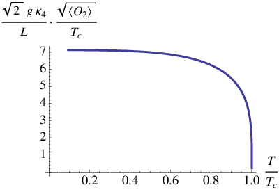
Without presenting the details of the analysis (see ref. [13]), we show in figure 1 the results of the variation of an order parameter as the temperature changes. The onset of superconductivity occurs for . The critical temperature is proportional to the square root of the charge density.
3.2 Perturbative limit
We now consider the scalar field as a perturbation about the dyonic black hole background. In this analysis, the Maxwell–scalar sector is not isolated from the gravity sector, since the Maxwell field has back–reacted on the gravitational background. We use the same potential considered in equation (7), which corresponds to choosing for the scalar field. Before proceeding with our analysis, we would like to emphasize the relationship between this work and that of ref. [13], which we reviewed in the previous section. We work in the limit where the scalar does not backreact on the Maxwell fields, which should correspond approximately to taking in ref. [13]. From equation (11), we see that this limit can be accomplished by taking . In this limit, the charge density diverges, and hence the limit corresponds to taking , i.e. the left most end of the curve in figure 1. This argument is further established by the fact that, in this regime, in the coupled equations studied in ref. [13] and reviewed earlier behaves almost linearly. In the dyonic black hole background, is linear. This suggests that the analysis we propose captures the physics at in ref. [13]. Therefore, for the physics we uncover, we are well below the critical temperature.
The equation of motion for the scalar field is given by:
| (13) |
The equation of motion for is simply the complex conjugate of equation (13). Using the fact that we only have and , and the only dependence is on the coordinates and , we consider an ansatz of the form . The equation of motion simplifies to:
| (14) |
This equation and its complex conjugate are purely real. Therefore, the equations of motion imply that the phase of is constant, and so without loss of generality, we take to be real. We assume a separable form for :
| (15) |
which further simplifies the equation of motion to:
| (16) | |||
where we have used the fact that . In order for this equation to be consistent, we must have that:
| (17) |
where is a constant. By changing to a dimensionless variable and setting , equation (17) can be brought to the form:
| (18) |
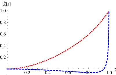
where . Generically, the solutions to this equation can be written in terms of confluent hypergeometric functions, but for the case when is an odd integer, the solutions can be written in terms of Hermite functions of order . We restrict ourselves to this case since the Hermite functions decay exponentially for large , which seems to be the natural physical choice. Henceforth in this paper, is taken to be an odd integer, and we display some examples of the functions in figure 2. However, in our present setup, we have assumed that the phase of the scalar field remains constant. Since only corresponds to a configuration that preserves its sign, it is the only physical solution for our ansatz.

As a result, our equation is exactly Schrödinger’s equation for a simple harmonic oscillator! Interestingly, the system confines the –extent of the condensate in a potential that is exactly quadratic. With the constant –field passing through the plane, we can compute the flux of through a region as:
| (19) |
Using the dimensionless variables we introduced earlier, we have:
| (20) |
only depends on since it is entirely determined by the behavior of the Hermite function. To estimate , we use that:
| (21) |
and , then our flux becomes:
| (22) |
where is the extent in the –direction, and since it is infinite there, we consider the flux per unit –length.
Substituting our result of equation (17) for the –dependence back into equation (16), the equation of motion for becomes:
| (23) |
Substituting in the functions, we get:
| (24) |
It is interesting to note that all and dependence in the equation have cancelled. This would seem to indicate that the scalar field’s behavior does not depend on and , but it is important to remember that we are working in the perturbative limit where is supposed to be small. Earlier, we stated that to ensure the perturbative limit is consistent, we must have the quantity to be large. Since the only dimensionful parameters are and , we take:
| (25) |
which ensures that the scalar field is always perturbative, and we can now work in terms of the dimensionless function .
Near the AdS boundary, equation (24) becomes:
| (26) |
which has the solution:
| (27) |
where and are dimensionless constants. Both of these solutions are normalizable, so one is not the source of the other. Having chosen by our choice of potential (see equation (7)), there is not a unique boundary condition at the AdS boundary [21]. is proportional to the vev of the operator () and is proportional to the vev of the operator () in the boundary field theory, and only one of these is turned on by the boundary condition. This forces us to pick as one of our boundary conditions:
| (28) |
We choose to only work with the , since we find the same general qualitative behavior for both operators. The exact relationship between the vev and the asymptotic value of can be calculated using the holographic dictionary (details are shown in Appendix A):
| (29) |
We can also study the behavior of the solution near the event horizon. We find that there are three distinct possible cases. First, if , then the equation of motion becomes:
| (30) |
where
which has Bessel functions as solutions:
| (31) | |||||
where is the Euler–Mascheroni constant. Since we want the field to be finite at the event horizon, we choose our other boundary condition to be . For , the equation of motion becomes
| (32) |
where
which has as solutions:
| (33) | |||||
Since we want the field to be finite at the event horizon, we would choose the same boundary condition as before, i.e. . Finally, if , we have:
| (34) |
where , which has as solutions:
| (35) | |||||
Again, if we want the field to be finite at the event horizon, we would choose the same boundary condition as before, i.e., .
4 Numerical Method and Results
There are several parameters that we can vary in this problem, . For the following analysis, we take for simplicity, but we can expect similar behavior for other values of . In order to solve equation (24), we use a shooting method. We impose the following initial conditions at the event horizon:
| (36) |
We find that these initial conditions do not necessarily satisfy equation (28). For a given , only for certain values of and do we get to satisfy the appropriate boundary conditions. Therefore, we fix the value of , and then scan through possible values of until the appropriate boundary condition at is satisfied, exhibiting our condensate.
We show in figure 3 two allowed solutions for the scalar field for a fixed and but with different values. Ref. [11] argues that only the zero--node solution matters to the phase structure, so we consider only these solutions in our subsequent analysis44 4 Indeed, we find that it is only for these zero–node solutions that persist for low enough temperature.. It is important to emphasize that changing the value of the scalar at the event horizon from the value given in equation (36) does not change the required value of and for the scalar to condense, but it does change the value of the vev. Therefore, at particular values of and that allow for a condensate to form, there is a whole range of allowed vev values for the operator depending on its value at the event horizon.
For convenience, we define a temperature (with its corresponding for which the scalar condenses) to be the temperature at zero magnetic field () at which we find a solution. This is given by (cf equation (3)):
| (37) |
Using this definition, we can define several dimensionless quantities of interest:
| (38) |
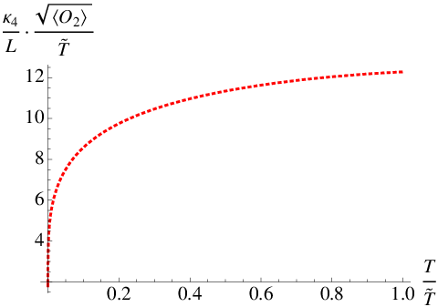
We present the results of our numerical condensate search in terms of these quantities in figure 4.


5 Discussion
As previously alluded to, since we are working in a limit where the scalar is not back–reacting on the Maxwell field, we cannot (as in ref.[13]) track the dependence of the vev on temperature all the way to the transition temperature55 5 Note that is not the transition temperature, but merely a normalization set by the solution at . . We instead simply exhibit the values of the ratios of temperature, charge density, and magnetic field to that allow a condensate to form in our study. This is enough to allow us to study the condensate’s spatial behavior, and we are firmly below in all that we do..
There are several interesting features, as displayed in figure 4. Note that in ref. [13], the scalar condenses at a particular value of , with . Similarly, the scalar in our setup condenses at a particular value of and . There exists a minimum value of for the scalar to condense. Beyond these values, condensation occurs but is not believed to be stable [11], and the only allowed solution is the trivial one (see the previous section for more details).
At zero magnetic field, the condensate fills the plane and requires the lowest ratio of . To see that it fills the plane, we recall that the profile in the –direction for is given by:
| (39) |
Therefore, in the limit of , we have , i.e. there is no –dependence. As the magnetic field is turned on and increases (reading the first and the other two plots from right to left as decreases), the value of required for the scalar to condense steadily increases and the condensate has a finite thickness along the –direction. At around , the ratio needed drops rapidly. The condensate also drops rapidly around the same interval, which suggests that the magnetic field might be overcoming the forces keeping the superconductor together. However, we find that even at , the condensate persists with a standard deviation of .
This result is of particular interest because, in the limit of large magnetic field, i.e. , the standard deviation approaches zero. Therefore, the magnetic field, as it grows, shrinks the condensate away completely. This is reminiscent of the Meissner effect, where the magnetic field expels the condensate. The condensate itself cannot expel the magnetic field, as is usually the case, since the scalar cannot back–react on the background magnetic field.
It is interesting to speculate on what higher values could mean if for example the ansatz for the scalar field is modified to make them physical. As an approximation, we can naively proceed with our setup with higher values of . We find that as increases and the –width of the condensate expands (see figure 2), the corresponding –field associated with it is smaller. It is interesting to follow this to large , the “classical” limit of the quantum harmonic oscillator controlling the –profile: The limit has the condensate filling the plane while the magnetic field . Pleasingly, this is consistent with the limit of small and large magnetic field we discussed above66 6 In making sense of the –field within the condensed region, where we expect it would be forced to zero in the fully back–reacting system, it is tempting to interpret the profile of the scalar quite literally and take times the average value within the region. This would mostly then integrate to zero in the interior of the sample, leaving only some non–zero contribution at the edges when is even, and canceling exactly when is odd, but this is possibly too naive..
Acknowledgments
TA thanks L’Institut de Physique Théorique (IPhT), Saclay, France for hospitality. He would also like to thank Nikolay Bobev and Hubert Saleur for discussions. This research was supported by the U.S. Department of Energy.
Appendix A Holographic Dictionary
The solution of the equation of motion admits two normalizable solutions at the AdS boundary, which we reproduce here:
To proceed with calculating the vev of the operator using the holographic dictionary, the procedure is to assume that is the source of the operator [21]. To proceed, we first write the asymptotic solution of the full scalar field as:
| (40) |
where we have explicitly shown the constant phase of the scalar field. Next, we calculate the variation of the on–shell action:
At this point, we may worry about the divergence produced by the first term in this expression, but we have not included the following counterterm in the expression of our action:
| (41) |
where is not the Euler–Mascheroni constant. Varying this counterterm and including it in the on–shell action gives as a final result:
| (42) |
Therefore, we have our final result:
| (43) |
where represents the fact that we want to study the operator in terms of unit length in the –direction. If we wish to only consider the overall scale of the operator (i.e., dropping the dependence), we can simply write:
| (44) |
References
- [1] J. M. Maldacena, “The large N limit of superconformal field theories and supergravity,” Adv. Theor. Math. Phys. 2 (1998) 231–252, hep-th/9711200.
- [2] S. S. Gubser, I. R. Klebanov, and A. M. Polyakov, “Gauge theory correlators from non-critical string theory,” Phys. Lett. B428 (1998) 105–114, hep-th/9802109.
- [3] E. Witten, “Anti-de Sitter space and holography,” Adv. Theor. Math. Phys. 2 (1998) 253–291, hep-th/9802150.
- [4] O. Aharony, S. S. Gubser, J. M. Maldacena, H. Ooguri, and Y. Oz, “Large N field theories, string theory and gravity,” Phys. Rept. 323 (2000) 183–386, hep-th/9905111.
- [5] R. M. Wald, “Black hole in a uniform magnetic field,” Phys. Rev. D10 (1974) 1680–1685.
- [6] J. Bicak and L. Dvorak, “Stationary Electromagnetic Fields Around Black Holes. 3. General Solutions and the Fields OF Current Loops Near the Reissner-Nordstrom Black Hole,” Phys. Rev. D22 (1980) 2933–2940.
- [7] A. Chamblin, R. Emparan, and G. W. Gibbons, “Superconducting p-branes and extremal black holes,” Phys. Rev. D58 (1998) 084009, hep-th/9806017.
- [8] R. Ruffini and J. A. Wheeler, “Introducing the black hole,” Physics Today 24 (1971) 30–41.
- [9] J. D. Bekenstein, “Black hole hair: Twenty-five years after,” gr-qc/9605059.
- [10] S. S. Gubser, “Phase transitions near black hole horizons,” Class. Quant. Grav. 22 (2005) 5121–5144, hep-th/0505189.
- [11] S. S. Gubser, “Breaking an Abelian gauge symmetry near a black hole horizon,” 0801.2977.
- [12] S. S. Gubser, “Colorful horizons with charge in anti-de Sitter space,” 0803.3483.
- [13] S. A. Hartnoll, C. P. Herzog, and G. T. Horowitz, “Building an AdS/CFT superconductor,” 0803.3295.
- [14] E. Nakano and W.-Y. Wen, “Critical magnetic field in AdS/CFT superconductor,” 0804.3180.
- [15] L. J. Romans, “Supersymmetric, cold and lukewarm black holes in cosmological Einstein-Maxwell theory,” Nucl. Phys. B383 (1992) 395–415, hep-th/9203018.
- [16] G. W. Gibbons and S. W. Hawking, “Classification Of Gravitational Instanton Symmetries,” Commun. Math. Phys. 66 (1979) 291–310.
- [17] S. Kobayashi, D. Mateos, S. Matsuura, R. C. Myers, and R. M. Thomson, “Holographic phase transitions at finite baryon density,” JHEP 02 (2007) 016, hep-th/0611099.
- [18] S. A. Hartnoll and P. Kovtun, “Hall conductivity from dyonic black holes,” Phys. Rev. D76 (2007) 066001, arXiv:0704.1160 [hep-th].
- [19] A. Chamblin, R. Emparan, C. V. Johnson, and R. C. Myers, “Charged AdS black holes and catastrophic holography,” Phys. Rev. D60 (1999) 064018, hep-th/9902170.
- [20] A. Chamblin, R. Emparan, C. V. Johnson, and R. C. Myers, “Holography, thermodynamics and fluctuations of charged AdS black holes,” Phys. Rev. D60 (1999) 104026, hep-th/9904197.
- [21] I. R. Klebanov and E. Witten, “AdS/CFT correspondence and symmetry breaking,” Nucl. Phys. B556 (1999) 89–114, hep-th/9905104.