跳到论文正文
W Papers独立论文阅读器 arXiv:0804.3453 论文正文 计算阅读时间 · 0%
引用这篇论文根据当前论文元数据生成,正式投稿前建议核对。


License: arXiv.org perpetual non-exclusive license
arXiv:0804.3453v1 [cs.IT] 22 Apr 2008

Weighted Sum Rate Optimization for Cognitive Radio MIMO Broadcast Channels
Thanks: The authors are with the Department of Electrical and Computer Engineering, National University of Singapore, Singapore 118622 (email: zhanglan@nus.edu.sg; elexy@nus.edu.sg). The corresponding author of the paper is Dr. Yan Xin (Tel. no: (65) 6516-5513 and Fax no. (65) 6779-1103).Thanks: ‡{{\ddagger}}The author is with Institute of Infocomm Research, 21 Heng Mui Keng Terrace, Singapore 119613 (email: ycliang@i2r.a-star.edu.sg).Thanks: Part of this work will be presented at IEEE International Conference on Communications, Beijing, China, May 2008.

Lan Zhang†, Yan Xin†*, and Ying-Chang Liang‡ Affiliation: EDICSSPC-APPL: Applications involving signal processing for communications
MSP-MULT: MIMO multi-user and multi-access schemes
Abstract

In this paper, we consider a cognitive radio (CR) network in which the unlicensed (secondary) users are allowed to concurrently access the spectrum allocated to the licensed (primary) users provided that their interference to the primary users (PUs) satisfies certain constraints. We study a weighted sum rate maximization problem for the secondary user (SU) multiple input multiple output (MIMO) broadcast channel (BC), in which the SUs have not only the sum power constraint but also interference constraints. We first transform this multi-constraint maximization problem into its equivalent form, which involves a single constraint with multiple auxiliary variables. Fixing these multiple auxiliary variables, we propose a duality result for the equivalent problem. Our duality result can solve the optimization problem for MIMO-BC with multiple linear constraints, and thus can be viewed as an extension of the conventional results, which rely crucially on a single sum power constraint. Furthermore, we develop an efficient sub-gradient based iterative algorithm to solve the equivalent problem and show that the developed algorithm converges to a globally optimal solution. Simulation results are further provided to corroborate the effectiveness of the proposed algorithm.

Index Terms: 
Beamforming, broadcast channel, cognitive radio, MIMO, power allocation, sum rate maximization.

I Introduction

Cognitive radio (CR), as a promising technology to advocate efficient use of radio spectrum, has been a topic of increasing research interest in recent years [1, 2, 3, 4, 5, 6, 7]. CR allows an unlicensed (secondary) user to opportunistically or concurrently access the spectrum initially allocated to the licensed (primary) users provided that certain prescribed constraints are satisfied, thus having a potential to improve spectral utilization efficiency. In this paper, we study a weighted sum rate maximization problem for the secondary user (SU) multiple input multiple output (MIMO) broadcast channel (BC) in a concurrent CR network, in which the SUs have not only the sum power constraint but also interference constraints.

I-A System Model and Problem Formulation

With reference to Fig. 1, we consider the KK-SU MIMO-BC with NtN_{t} transmit antennas and NrN_{r} receive antennas in a CR network, where the KK SUs share the same spectrum with a single primary user (PU) equipped with one transmitter and one receiver11 1 Expect for explicitly stated, we restrict our attention to a single PU case in the rest of this paper for convenience of description. The results derived for the single PU case can be readily extended to the multiple PU case, which is discussed in Remark 4.. The transmit-receive signal model from the BS to the iith SU denoted by SUi, for i=1,…,Ki=1,\ldots,K, can be expressed as

𝒚i=𝑯i​𝒙+𝒛i,{\mbox{\boldmath$y$}}_{i}={\mbox{\boldmath$H$}}_{i}{\mbox{\boldmath$x$}}+{\mbox{\boldmath$z$}}_{i}, (1)

where 𝒚i{\mbox{\boldmath$y$}}_{i} is the Nr×1N_{r}\times 1 received signal vector, 𝑯i{\mbox{\boldmath$H$}}_{i} is the Nr×NtN_{r}\times N_{t} channel matrix from the BS to the SUi, 𝒙x is the Nt×1N_{t}\times 1 transmitted signal vector, and 𝒛i{\mbox{\boldmath$z$}}_{i} is the Nr×1N_{r}\times 1 Gaussian noise vector with entries being independent identically distributed random variables (RVs) with mean zero and variance σ2\sigma^{2}. Consider 𝒉o{\mbox{\boldmath$h$}}_{o} as the Nt×1N_{t}\times 1 channel gain vector between the transmitters of the BS and the PU. We further assume that 𝑯i{\mbox{\boldmath$H$}}_{i} for i=1,…,Ki=1,\ldots,K, and 𝒉o{\mbox{\boldmath$h$}}_{o} remain constant during a transmission block and change independently from block to block, and 𝑯i{\mbox{\boldmath$H$}}_{i} for i=1,…,Ki=1,\ldots,K, and 𝒉o{\mbox{\boldmath$h$}}_{o} are perfectly known to the BS and SUi. This requires that the SUs can “cognitively” obtain the information of its neighboring environment. In practice, certain cooperation in terms of parameter feedback between the PU and the BS is needed. To achieve that, the protocol for the SU network can be designed as follows: every frame contains sensing sub-frame and data transmission sub-frame. During the sensing sub-frame, BS can transmit training sequences to SUs as well as to the PU so that the SUs can estimate the channel matrix 𝑯i{\mbox{\boldmath$H$}}_{i}, and the PU can measure the vector 𝒉o{\mbox{\boldmath$h$}}_{o}. After that, this information will be sent back to the BS via a feedback channel.

We next consider the weighted sum rate maximization problem for the KK-SU MIMO-BC in a CR network, simply called the CR MIMO-BC sum rate maximization problem, which, mathematically, can be formulated as

Problem 1 (Main Problem)
max{𝑸ib}i=1K:𝑸ib⪰0\displaystyle\underset{{\{{\mbox{\small\boldmath$Q$}}_{i}^{\text{b}}\}_{i=1}^{K}:~{\mbox{\small\boldmath$Q$}}^{\text{b}}_{i}\succeq 0}}{\text{max}}~ ∑i=1Kwi​rib\displaystyle\sum_{i=1}^{K}w_{i}r_{i}^{\text{b}} (2)
subject to   ∑i=1K𝒉o†​𝑸ib​𝒉o≤Pt,and​∑i=1Ktr​(𝑸ib)≤Pu,\displaystyle\sum_{i=1}^{K}{\mbox{\boldmath$h$}}_{o}^{{\dagger}}{\mbox{\boldmath$Q$}}_{i}^{\text{b}}{\mbox{\boldmath$h$}}_{o}\leq P_{t},~\text{and}~\sum_{i=1}^{K}\text{tr}({\mbox{\boldmath$Q$}}_{i}^{\text{b}})\leq P_{u},

where ribr_{i}^{\text{b}} is the rate achieved by SUi, wiw_{i} is the weight of SUi, 𝑸ib{\mbox{\boldmath$Q$}}_{i}^{\text{b}} denotes the Nt×NtN_{t}\times N_{t} transmit signal covariance matrix for SUi, 𝑸ib⪰0{\mbox{\boldmath$Q$}}_{i}^{\text{b}}\succeq 0 denotes that 𝑸ib{\mbox{\boldmath$Q$}}_{i}^{\text{b}} is a semidefinite matrix, PtP_{t} denotes the interference threshold of the PU, and PuP_{u} denotes the sum power constraint at the BS. In a non-CR setting, similar weighted sum rate optimization problems for the multiple input single output (MISO) BC and the MIMO-BC have been studied in [8][9], respectively. The key difference is that in addition to the sum power constraint, an interference constraint is applied to the SUs in the CR MIMO-BC, i.e., the total received interference power ∑i=1K𝒉o†​𝑸ib​𝒉o\sum_{i=1}^{K}{\mbox{\boldmath$h$}}_{o}^{{\dagger}}{\mbox{\boldmath$Q$}}_{i}^{\text{b}}{\mbox{\boldmath$h$}}_{o} at the PU is below the threshold PtP_{t}.

Remark 1

It has long been observed that the optimal sum rate for MIMO BC with a single sum power constraint is equal to the optimal sum rate of the dual MIMO multiple access channel (MAC) with the same sum power constraint [10][11][12]. However, this conventional BC-MAC duality can only be applied to the case with a single sum power constraint (even not applicable to an arbitrary linear power constraint). Hence, the additional interference power constraint in Problem 1 makes the existing duality cannot be applied. The new duality result proposed in this paper generalizes the previous results as special cases. Moreover, it is worth to note that any boundary point of the capacity regions of the MIMO-MAC and the MIMO-BC can be expressed as a weighted sum rate for a certain choice of weights [13] [14]. Thus, by varying the weights of the SUs in Problem 1, the entire capacity region of the CR MIMO-BC can be obtained.

I-B Related Work

The present paper is motivated by the previous work on the information-theoretic study of the MIMO-BC under a non-CR setting. It has been shown in [11][12][15] that under a single sum power constraint, the sum-capacity of the non-CR MIMO-BC can be achieved by the dirty paper coding (DPC) scheme. Furthermore, the paper [16] shows that the rate region achieved by the DPC scheme is indeed the capacity region of such a channel. However, the power allocation and beamforming strategies to achieve the capacity region have been not considered in these papers. Moreover, it has been shown in [17][18] that under the single sum power constraint, the equally weighted sum rate maximization problem, simply called the sum rate problem, for the MIMO-BC can be solved by solving its dual MIMO MAC sum rate problem, which is also subject to a single sum power constraint. In [17], a cyclic coordinate ascent algorithm was proposed to solve the dual MIMO-MAC problem while in [18] this sum-power constrained dual problem was decoupled into an individual-power constrained problem, which can be solved by using an iterative water-filling algorithm [19]. Even though these algorithms proposed in [17][18] can solve the sum rate optimization problem for the non-CR MIMO-BC via the MAC-BC duality, they are not applicable to the general weighted sum rate problem. In [8], a generalized iterative water-filling was proposed to solve the weighted sum rate problem for the MISO-BC where each user has a single receive antenna. However, the proposed algorithm is not applicable to the general MIMO-BC case. Furthermore, an efficient algorithm was proposed to solve the MIMO-BC weighted sum rate problem with a single sum power constraint in [9]. These aforementioned results are based on the conventional BC-MAC duality, which cannot be applied to solve the weighted sum rate problem with multiple constraints (the case of interest in this paper). Recently, the paper [20] investigated a different MIMO-BC weighted sum rate maximization problem which is subject to per-antenna power constraints instead of the single sum power constraint, and established a new minimax duality which is different from the conventional BC-MAC duality. A Newton’s method based algorithm was proposed to solve this minimax problem. In this paper, we consider a more general case where the power is subject to multiple linear constraints instead of the sum power constraint or per-antenna power constraints, and propose a new BC-MAC duality result to extend the conventional duality result so that it can solve the problem with multiple arbitrary linear constraints. A Karush-Kuhn-Tucker (KKT) condition based algorithm is developed to solve the problem.

I-C Contribution

Throughout the paper, we consider the CR MIMO-BC weighted sum rate maximization problem as defined in Problem 1. As the main contribution of this paper, our solution is summarized in the following.

  1. 1.

    We prove that in the CR MIMO-BC, the multi-constraint weighted sum rate maximization problem (Problem 1) is equivalent to a single-constraint weighted sum rate maximization problem with multiple auxiliary variables.

  2. 2.

    For the equivalent problem, we establish a duality between the MIMO-BC and a dual MIMO-MAC when the multiple auxiliary variables are fixed as constant. This duality is applicable to MIMO-BC with arbitrary linear power constraint, and can be viewed as an extension of the conventional MIMO MAC-BC duality result [10][11][12], which is only valid for the problem with a single sum power constraint.

  3. 3.

    For the weighted sum rate maximization problem of the dual MIMO MAC, the existing iterative water-filling based algorithm [17, 18] is not applicable. We propose a new primal dual method based iterative algorithm [21] to solve it. Furthermore, we propose a sub-gradient based iterative algorithm to solve the main problem of the paper, Problem 1, and show that the proposed algorithm converges to the globally optimal solution.

I-D Organization and Notation

The rest of the paper is organized as follows. In Section II, we transform the CR MIMO-BC weighted sum rate maximization problem (Problem 1) into its equivalent form, and introduce a MAC-BC duality between a MIMO-BC and a dual MIMO-MAC. Section III presents an primal dual method based iterative algorithm to solve the dual MIMO-MAC weighted sum rate problem. In Section IV, a MAC-BC covariance matrix mapping algorithm is proposed. Section V presents the complete algorithm to solve the CR MIMO-BC weighted sum rate maximization problem. Section VI provides several simulation examples. Finally, Section VII concludes the paper.

The following notations are used in this paper. The boldface is used to denote matrices and vectors, (⋅)†(\cdot)^{{\dagger}} and (⋅)T(\cdot)^{T} denote the conjugate transpose and transpose, respectively; 𝑰M{{\mbox{\boldmath$I$}}}_{M} denotes an M×MM\times M identity matrix; tr​(⋅)\text{tr}(\cdot) denotes the trace of a matrix, and [x]+[x]^{+} denotes max⁡(x,0)\max(x,0); (⋅)b(\cdot)^{\text{b}} and (⋅)m(\cdot)^{\text{m}} denote the quantities associated with a broadcast channel and a multiple access channel, respectively; E⁡[⋅]E[\cdot] denotes the expectation operator.

II Equivalence and Duality

Evidently, the MIMO-BC weighted sum rate maximization problem under either a non-CR or a CR setting is a non-convex optimization problem and is difficult to solve directly. Under a single sum power constraint, the weighted sum rate problem for MIMO BC can be transformed to its dual MIMO MAC problem, which is convex and can be solved in an efficient manner [8][9]. In the CR setting, the problem (Problem 1) has not only a sum power constraint but also an interference constraint. The imposed multiple constraints render difficulty to formulate an efficiently solvable dual problem. To overcome the difficulty, we first transform this multi-constrained weighted sum rate problem (Problem 1) into its equivalent problem which has a single constraint with multiple auxiliary variables, and next develop a duality between a MIMO-BC and a dual MIMO-MAC in the case where the multiple auxiliary variables are fixed.

II-A An Equivalent MIMO-BC Weighted Sum Rate Problem

In the following proposition, we present an equivalent form of Problem 1 (see Appendix B for the proof).

Proposition 1

Problem 1 shares the same optimal solution with

Problem 2 (Equivalent Problem)
minqt≥0,qu≥0max{𝑸ib}i=1K:𝑸ib⪰0∑i=1Kwirib\displaystyle\underset{q_{t}\geq 0,~q_{u}\geq 0}{\text{min}}\underset{{\{{\mbox{\small\boldmath$Q$}}_{i}^{\text{b}}\}_{i=1}^{K}:~{\mbox{\small\boldmath$Q$}}^{\text{b}}_{i}\succeq 0}}{\text{max}}~\sum_{i=1}^{K}w_{i}r_{i}^{\text{b}} (3)
subject to ​qt​(∑i=1K𝒉o†​𝑸ib​𝒉o−Pt)+qu​(∑i=1Ktr​(𝑸ib)−Pu)≤0,\displaystyle\text{subject to~}~q_{t}\big(\sum_{i=1}^{K}{\mbox{\boldmath$h$}}_{o}^{{\dagger}}{\mbox{\boldmath$Q$}}_{i}^{\text{b}}{\mbox{\boldmath$h$}}_{o}-P_{t}\big)+q_{u}\big(\sum_{i=1}^{K}\text{tr}({\mbox{\boldmath$Q$}}_{i}^{\text{b}})-P_{u}\big)\leq 0, (4)

where qtq_{t} and quq_{u} are the auxiliary dual variables for the respective interference constraint and sum power constraint.

It can be readily concluded from the proposition that the optimal solution to Problem 2 also satisfies ∑i=1K𝒉o†​𝑸ib​𝒉o≤Pt\sum_{i=1}^{K}{\mbox{\boldmath$h$}}_{o}^{{\dagger}}{\mbox{\boldmath$Q$}}_{i}^{\text{b}}{\mbox{\boldmath$h$}}_{o}\leq P_{t} and ∑i=1Ktr​(𝑸ib)≤Pu\sum_{i=1}^{K}\text{tr}({\mbox{\boldmath$Q$}}_{i}^{\text{b}})\leq P_{u} simultaneously since it is also the optimal solution to Problem 1. Finding an efficiently solvable dual problem for Problem 2 directly is still difficult. However, as we show later, when qtq_{t} and quq_{u} are fixed as constants, Problem 2 reduces to a simplified form, which we can solve by applying the following duality result.

II-B CR MIMO BC-MAC Duality

For fixed qtq_{t} and quq_{u}, Problem 2 reduces to the following form

Problem 3 (CR MIMO-BC)
max{𝑸ib}i=1K:𝑸ib⪰0\displaystyle\underset{{\{{\mbox{\small\boldmath$Q$}}_{i}^{\text{b}}\}_{i=1}^{K}:~{\mbox{\small\boldmath$Q$}}^{\text{b}}_{i}\succeq 0}}{\text{max}}~ ∑i=1Kwi​rib\displaystyle\sum_{i=1}^{K}w_{i}r_{i}^{\text{b}} (5)
subject to ​qt\displaystyle\text{subject to~}~q_{t} ∑i=1K𝒉o†​𝑸ib​𝒉o+qu​∑i=1Ktr​(𝑸ib)≤P,\displaystyle\sum_{i=1}^{K}{\mbox{\boldmath$h$}}_{o}^{{\dagger}}{\mbox{\boldmath$Q$}}_{i}^{\text{b}}{\mbox{\boldmath$h$}}_{o}+q_{u}\sum_{i=1}^{K}\text{tr}({\mbox{\boldmath$Q$}}_{i}^{\text{b}})\leq P, (6)

where P:=qt​Pt+qu​PuP:=q_{t}P_{t}+q_{u}P_{u}. Since qtq_{t} and quq_{u} are fixed, PP is a constant in Problem 3. The constraint (6) is not a single sum power constraint, and thus the duality result established in [17] is not applicable to Problem 3. Therefore, we formulate the following new dual MAC problem.

Proposition 2

The dual MAC problem of Problem 3 is

Problem 4 (CR MIMO-MAC)
max{𝑸im}i=1K:𝑸im⪰0\displaystyle\underset{{\{{\mbox{\small\boldmath$Q$}}_{i}^{\text{m}}\}_{i=1}^{K}:~{\mbox{\small\boldmath$Q$}}^{\text{m}}_{i}\succeq 0}}{\text{max}}~ ∑i=1Kwi​rim\displaystyle\sum_{i=1}^{K}w_{i}r_{i}^{\text{m}} (7)
subject to   ∑i=1Ktr​(𝑸im)​σ2≤P,\displaystyle\sum_{i=1}^{K}\text{tr}({\mbox{\boldmath$Q$}}_{i}^{\text{m}})\sigma^{2}\leq P, (8)

where rimr_{i}^{\text{m}} is the rate achieved by the iith user of the dual MAC, 𝑸im{\mbox{\boldmath$Q$}}_{i}^{\text{m}} is the transmit signal covariance matrix of the iith user, and the noise covariance at the BS is qt​𝒉o​𝒉oH+qu​𝑰Ntq_{t}{\mbox{\boldmath$h$}}_{o}{\mbox{\boldmath$h$}}_{o}^{H}+q_{u}{\mbox{\boldmath$I$}}_{N_{t}}.

Remark 2

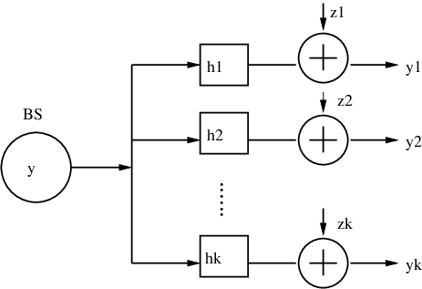
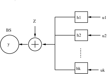
According to Proposition 2, for fixed qtq_{t} and quq_{u}, the optimal weighted sum rate of the dual MAC is equal to the optimal weighted sum rate of the primal BC. From the formulation perspective, this duality result is quite similar to the conventional duality in [10][11][12]. However, as shown in Fig. 2, one thing needs to highlight is that the noise covariance matrix of the dual MAC is a function of the auxiliary variable qtq_{t} and quq_{u}, instead of the identity matrix [12]. This difference comes from the constraint (6), which is not a sum power constraint as in [12]. Note that when qt=0q_{t}=0, the duality result reduces to the conventional BC-MAC duality in [12].

As illustrated in Fig. 2, Proposition 2 describes a weighted sum rate maximization problem for a dual MIMO-MAC. To prove the proposition, we first examine the relation between the signal to interference plus noise ratio (SINR) regions of the MIMO-BC and the dual MIMO-MAC. Based on this relation, we will show that the achievable rate regions of the MIMO-BC and the dual MIMO-MAC are the same.

In the sequel, we first describe the definition of the SINR for the MIMO-BC. It has been shown in [16] that the DPC is a capacity achieving scheme. Each set of the transmit covariance matrix determined by DPC scheme defines a set of transmit and receive beamforming vectors, and each pair of these transmit and receive beamforming vectors forms a data stream. In a beamforming perspective, the BS transmitter have Nt×KN_{t}\times K beamformers, 𝒖i,j{\mbox{\boldmath$u$}}_{i,j}, for i=1,⋯,Ki=1,\cdots,K, and j=1,⋯,Ntj=1,\cdots,N_{t}. Therefore, the transmit signal can be represented as

𝒙=∑i=1K∑j=1Ntxi,j​𝒖i,j,{\mbox{\boldmath$x$}}=\sum_{i=1}^{K}\sum_{j=1}^{N_{t}}x_{i,j}{\mbox{\boldmath$u$}}_{i,j},

where xi,jx_{i,j} is a scalar representing the data stream transmitted in this beamformer, and E⁡[xi,j2]=pi,jE[x_{i,j}^{2}]=p_{i,j} denotes the power allocated to this beamformer. At SUi, the receive beamformer corresponding to 𝒖i,j{\mbox{\boldmath$u$}}_{i,j} is denoted by 𝒗i,j{\mbox{\boldmath$v$}}_{i,j}. The transmit beamformer 𝒖i,j{\mbox{\boldmath$u$}}_{i,j} and the power pi,jp_{i,j} can be obtained via the eigenvalue decomposition of 𝑸ib{\mbox{\boldmath$Q$}}_{i}^{\text{b}}, i.e., 𝑸ib=𝑼i†​𝑷i​𝑼i{\mbox{\boldmath$Q$}}_{i}^{\text{b}}={\mbox{\boldmath$U$}}_{i}^{{\dagger}}{\mbox{\boldmath$P$}}_{i}{\mbox{\boldmath$U$}}_{i}, where 𝑼i{\mbox{\boldmath$U$}}_{i} is a unitary matrix, and 𝑷i{\mbox{\boldmath$P$}}_{i} is a diagonal matrix. The transmit beamformer 𝒖i,j{\mbox{\boldmath$u$}}_{i,j} is the jjth column of 𝑼i{\mbox{\boldmath$U$}}_{i}, and pi,jp_{i,j} is the jjth diagonal entry of 𝑷i{\mbox{\boldmath$P$}}_{i}. With these notations, we express the SINRi,jb\text{SINR}_{i,j}^{\text{b}} as

SINRi,jb=pi,j​|𝒖i,j†​𝑯i†​𝒗i,j|2∑k=i+1K∑l=1Nrpk,l​|𝒖k,l†​𝑯i†​𝒗i,j|2+∑l=j+1Nrpi,l​|𝒖i,l†​𝑯i†​𝒗i,j|2+σ2.\text{SINR}_{i,j}^{\text{b}}=\frac{p_{i,j}|{\mbox{\boldmath$u$}}_{i,j}^{{\dagger}}{\mbox{\boldmath$H$}}_{i}^{{\dagger}}{\mbox{\boldmath$v$}}_{i,j}|^{2}}{\sum_{k=i+1}^{K}\sum_{l=1}^{N_{r}}p_{k,l}|{\mbox{\boldmath$u$}}_{k,l}^{{\dagger}}{\mbox{\boldmath$H$}}_{i}^{{\dagger}}{\mbox{\boldmath$v$}}_{i,j}|^{2}+\sum_{l=j+1}^{N_{r}}p_{i,l}|{\mbox{\boldmath$u$}}_{i,l}^{{\dagger}}{\mbox{\boldmath$H$}}_{i}^{{\dagger}}{\mbox{\boldmath$v$}}_{i,j}|^{2}+\sigma^{2}}. (9)

It can be observed from (9) that the DPC scheme is applied. This can be interpreted as follows. The signal from SU1 is first encoded with the signals from other SUs being treated as interference. The signal from SU2 is next encoded by using the DPC scheme. Signals from the other SUs will be encoded sequentially in a similar manner. For the data streams within SUi, the data stream 1 is also encoded first while the other data streams are treated as the interference. The data stream 2 is encoded next. In a similar manner, the other data streams will be sequentially encoded. The encoding order is assumed to be arbitrary at this moment, and the optimal encoding order of Problem 2 will be discussed in Section III.

To explore the relation of the SINR regions of the dual MAC and the BC, we formulate a following optimization problem

min{𝑸ib}i=1K:𝑸ib⪰0qt​∑i=1K𝒉o†​𝑸ib​𝒉o+qu​∑i=1Ktr​(𝑸ib)−Psubject to SINRi,jb≥γi,j,\displaystyle\begin{split}\underset{{\{{\mbox{\small\boldmath$Q$}}_{i}^{\text{b}}\}_{i=1}^{K}:~{\mbox{\small\boldmath$Q$}}^{\text{b}}_{i}\succeq 0}}{\text{min}}~&q_{t}\sum_{i=1}^{K}{\mbox{\boldmath$h$}}_{o}^{{\dagger}}{\mbox{\boldmath$Q$}}_{i}^{\text{b}}{\mbox{\boldmath$h$}}_{o}+q_{u}\sum_{i=1}^{K}\text{tr}({\mbox{\boldmath$Q$}}_{i}^{\text{b}})-P\\ \text{subject to~}~&\text{SINR}_{i,j}^{\text{b}}\geq\gamma_{i,j},\end{split} (10)

where γi,j\gamma_{i,j} denotes the SINR threshold of the jjth data stream within the SUi for the BC. Note that the objective function in (10) is a function of signal covariance matrices and the constraints are SINR constraints for the KK-SU MIMO-BC.

It has been shown in [20] and [22] that the non-convex BC sum power minimization problem under the SINR constraints can be solved efficiently via its dual MAC problem, which is a convex optimization problem. By following a similar line of thinking, the problem in (10) can be efficiently solved via its dual MAC problem. Similar to the primal MIMO-BC, the dual MIMO-MAC depicted in Fig. 2 consists of KK users each with NrN_{r} transmit antennas, and one BS with NtN_{t} receive antennas. By transposing the channel matrix and interchanging the input and output signals, we obtain the dual MIMO-MAC from the primal MIMO-BC. For the covariance matrices 𝑸im{\mbox{\boldmath$Q$}}_{i}^{\text{m}} of the dual MIMO-MAC, we apply the eigenvalue decomposition,

𝑸im=𝑽i​𝚲i​𝑽i†=∑j=1Nrqi,j​𝒗i,j​𝒗i,j†,{\mbox{\boldmath$Q$}}^{\text{m}}_{i}={\mbox{\boldmath$V$}}_{i}{\bf\Lambda}_{i}{\mbox{\boldmath$V$}}^{{\dagger}}_{i}=\sum_{j=1}^{N_{r}}q_{i,j}{\mbox{\boldmath$v$}}_{i,j}{\mbox{\boldmath$v$}}_{i,j}^{{\dagger}}, (11)

where 𝒗i,j{\mbox{\boldmath$v$}}_{i,j} is the jjth column of 𝑽i{\mbox{\boldmath$V$}}_{i}, and qi,jq_{i,j} is the jjth diagonal entry of 𝚲i{\bf{\Lambda}}_{i}. For user ii, 𝒗i,j{\mbox{\boldmath$v$}}_{i,j} is the transmit beamforming vector of the jjth data stream, the power allocated to the jjth data stream equals qi,jq_{i,j}, and the receive beamforming vector of the jjth data stream at the BS is 𝒖i,j{\mbox{\boldmath$u$}}_{i,j}. The SINR of the dual MIMO-MAC is given by

SINRi,jm=qi,j​|𝒖i,j†​𝑯i†​𝒗i,j|2𝒖i,j†​(∑k=1i−1∑l=1Nrqk,l​𝑯k†​𝒗k,l​𝒗k,l†​𝑯k+∑l=1j−1qi,l​𝑯i†​𝒗i,l​𝒗i,l†​𝑯i+𝑹w)​𝒖i,j,\text{SINR}_{i,j}^{\text{m}}=\frac{q_{i,j}|{\mbox{\boldmath$u$}}_{i,j}^{{\dagger}}{\mbox{\boldmath$H$}}_{i}^{{\dagger}}{\mbox{\boldmath$v$}}_{i,j}|^{2}}{{\mbox{\boldmath$u$}}_{i,j}^{{\dagger}}\left(\sum_{k=1}^{i-1}\sum_{l=1}^{N_{r}}q_{k,l}{\mbox{\boldmath$H$}}_{k}^{{\dagger}}{\mbox{\boldmath$v$}}_{k,l}{\mbox{\boldmath$v$}}_{k,l}^{{\dagger}}{\mbox{\boldmath$H$}}_{k}+\sum_{l=1}^{j-1}q_{i,l}{\mbox{\boldmath$H$}}_{i}^{{\dagger}}{\mbox{\boldmath$v$}}_{i,l}{\mbox{\boldmath$v$}}_{i,l}^{{\dagger}}{\mbox{\boldmath$H$}}_{i}+{\mbox{\boldmath$R$}}_{w}\right){\mbox{\boldmath$u$}}_{i,j}}, (12)

where 𝑹w:=qt​𝑹o+qu​𝑰Nt{\mbox{\boldmath$R$}}_{w}:=q_{t}{\mbox{\boldmath$R$}}_{o}+q_{u}{\mbox{\boldmath$I$}}_{N_{t}} is the noise covariance matrix of the MIMO-MAC with 𝑹o:=𝒉o​𝒉o†{\mbox{\boldmath$R$}}_{o}:={\mbox{\boldmath$h$}}_{o}{\mbox{\boldmath$h$}}_{o}^{{\dagger}}. In the dual MIMO-MAC, 𝑹w{\mbox{\boldmath$R$}}_{w} depends on qtq_{t} and quq_{u} defined in (10) whereas the noise covariance matrix in the primal MIMO-BC is an identity matrix. It can be observed from (12) that the successive interference cancelation (SIC) scheme is used in this dual MIMO-MAC, and the decoding order is the reverse encoding order of the primal BC. The signal from SUK is first decoded with the signals from other users being treated as interference. After decoded at the BS, the signals from SUK will be subtracted from the received signal. The signal from SUK-1 is next decoded, and so on. Again, the data streams within a SU can be decoded in a sequential manner.

For the dual MIMO-MAC, we consider the following minimization problem similar to the problem (10)

min{𝑸im}i=1K:𝑸im⪰0∑i=1Ktr​(𝑸im)​σ2−Psubject to SINRi,jm≥γi,j.\displaystyle\begin{split}\underset{{\{{\mbox{\small\boldmath$Q$}}_{i}^{\text{m}}\}_{i=1}^{K}:~{\mbox{\small\boldmath$Q$}}^{\text{m}}_{i}\succeq 0}}{\text{min}}~&\sum_{i=1}^{K}\text{tr}({\mbox{\boldmath$Q$}}_{i}^{\text{m}})\sigma^{2}-P\\ \text{subject to~}~&\text{SINR}_{i,j}^{\text{m}}\geq\gamma_{i,j}.\end{split} (13)

The following proposition describes the relation between the problems (10) and (13).

Proposition 3

For fixed qtq_{t} and quq_{u}, the MIMO-MAC problem (13) is dual to the MIMO-BC problem (10).

Proof:

The constraints in (10) can be rewritten as

pi,j​|𝒖i,j†​𝑯i†​𝒗i,j|2γi,j≥∑k=i+1K∑l=1Nrpk,l​|𝒖k,l†​𝑯i†​𝒗i,j|2+∑l=j+1Nrpi,l​|𝒖i,l†​𝑯i†​𝒗i,j|2+σ2.\displaystyle\frac{p_{i,j}|{\mbox{\boldmath$u$}}_{i,j}^{{\dagger}}{\mbox{\boldmath$H$}}_{i}^{{\dagger}}{\mbox{\boldmath$v$}}_{i,j}|^{2}}{\gamma_{i,j}}\!\geq\!\sum_{k=i+1}^{K}\sum_{l=1}^{N_{r}}p_{k,l}|{\mbox{\boldmath$u$}}_{k,l}^{{\dagger}}{\mbox{\boldmath$H$}}_{i}^{{\dagger}}{\mbox{\boldmath$v$}}_{i,j}|^{2}\!+\!\sum_{l=j+1}^{N_{r}}p_{i,l}|{\mbox{\boldmath$u$}}_{i,l}^{{\dagger}}{\mbox{\boldmath$H$}}_{i}^{{\dagger}}{\mbox{\boldmath$v$}}_{i,j}|^{2}+\sigma^{2}. (14)

Thus, the Lagrangian function of the problem (10) is

L1​(𝑸1b,…,𝑸Kb,λi,j)\displaystyle L_{1}({\mbox{\boldmath$Q$}}^{\text{b}}_{1},\ldots,{\mbox{\boldmath$Q$}}^{\text{b}}_{K},\lambda_{i,j})
=\displaystyle= qt​∑i=1K𝒉o†​𝑸ib​𝒉o+qu​∑i=1Ktr​(𝑸ib)−P−∑i=1K∑j=1Nrλi,j​(pi,j​|𝒖i,j†​𝑯i†​𝒗i,j|2γi,jCLOSE\displaystyle q_{t}\sum_{i=1}^{K}{\mbox{\boldmath$h$}}_{o}^{{\dagger}}{\mbox{\boldmath$Q$}}_{i}^{\text{b}}{\mbox{\boldmath$h$}}_{o}+q_{u}\sum_{i=1}^{K}\text{tr}({\mbox{\boldmath$Q$}}_{i}^{\text{b}})-P-\sum_{i=1}^{K}\sum_{j=1}^{N_{r}}\lambda_{i,j}\Big(\frac{p_{i,j}|{\mbox{\boldmath$u$}}_{i,j}^{{\dagger}}{\mbox{\boldmath$H$}}_{i}^{{\dagger}}{\mbox{\boldmath$v$}}_{i,j}|^{2}}{\gamma_{i,j}}
−∑k=i+1K∑l=1Nrpk,l|𝒖k,l†𝑯i†𝒗i,j|2−∑l=j+1Nrpi,l|𝒖i,l†𝑯i†𝒗i,j|2−σ2)\displaystyle-\sum_{k=i+1}^{K}\sum_{l=1}^{N_{r}}p_{k,l}|{\mbox{\boldmath$u$}}_{k,l}^{{\dagger}}{\mbox{\boldmath$H$}}_{i}^{{\dagger}}{\mbox{\boldmath$v$}}_{i,j}|^{2}-\sum_{l=j+1}^{N_{r}}p_{i,l}|{\mbox{\boldmath$u$}}_{i,l}^{{\dagger}}{\mbox{\boldmath$H$}}_{i}^{{\dagger}}{\mbox{\boldmath$v$}}_{i,j}|^{2}-\sigma^{2}\Big) (15)
=\displaystyle= ∑i=1K∑j=1Nrλi,j​σ2−P−∑i=1K∑j=1Nrpi,j​𝒖i,j†​(λi,j​𝑯i†​𝒗i,j​𝒗i,j†​𝑯iγi,jCLOSE\displaystyle\sum_{i=1}^{K}\sum_{j=1}^{N_{r}}\lambda_{i,j}\sigma^{2}-P-\sum_{i=1}^{K}\sum_{j=1}^{N_{r}}p_{i,j}{\mbox{\boldmath$u$}}_{i,j}^{{\dagger}}\Big(\frac{\lambda_{i,j}{\mbox{\boldmath$H$}}_{i}^{{\dagger}}{\mbox{\boldmath$v$}}_{i,j}{\mbox{\boldmath$v$}}_{i,j}^{{\dagger}}{\mbox{\boldmath$H$}}_{i}}{\gamma_{i,j}}
−∑k=1i−1∑l=1Nrλk,l𝑯k†𝒗k,l𝒗k,l†𝑯k−∑l=1j−1λi,l𝑯i†𝒗i,l𝒗i,l†𝑯i−𝑹w)𝒖i,j,\displaystyle-\sum_{k=1}^{i-1}\sum_{l=1}^{N_{r}}\lambda_{k,l}{\mbox{\boldmath$H$}}_{k}^{{\dagger}}{\mbox{\boldmath$v$}}_{k,l}{\mbox{\boldmath$v$}}_{k,l}^{{\dagger}}{\mbox{\boldmath$H$}}_{k}-\sum_{l=1}^{j-1}\lambda_{i,l}{\mbox{\boldmath$H$}}_{i}^{{\dagger}}{\mbox{\boldmath$v$}}_{i,l}{\mbox{\boldmath$v$}}_{i,l}^{{\dagger}}{\mbox{\boldmath$H$}}_{i}-{\mbox{\boldmath$R$}}_{w}\Big){\mbox{\boldmath$u$}}_{i,j}, (16)

where λi,j\lambda_{i,j} is the Lagrangian multiplier. Eq. (16) is obtained by applying the eigenvalue decomposition to 𝑸ib{\mbox{\boldmath$Q$}}_{i}^{\text{b}} and rearranging the terms in (15). The optimal objective value of (10) is

maxλi,j​min𝑸1b,…,𝑸Kb​L1​(𝑸1b,…,𝑸Kb,λi,j).\underset{\lambda_{i,j}}{\text{max}}\underset{{\mbox{\small\boldmath$Q$}}^{\text{b}}_{1},\ldots,{\mbox{\small\boldmath$Q$}}^{\text{b}}_{K}}{\text{min}}L_{1}({\mbox{\boldmath$Q$}}^{\text{b}}_{1},\ldots,{\mbox{\boldmath$Q$}}^{\text{b}}_{K},\lambda_{i,j}). (17)

On the other hand, the Lagrangian function of the problem (13) is

L2​(𝑸1m,…,𝑸Km,δi,j)=∑i=1K∑j=1Nrqi,j​σ2−P−∑i=1K∑j=1Nrδi,j​𝒖i,j†​(qi,j​𝑯i†​𝒗i,j​𝒗i,j†​𝑯iγi,jCLOSE\displaystyle L_{2}({\mbox{\boldmath$Q$}}^{\text{m}}_{1},\ldots,{\mbox{\boldmath$Q$}}^{\text{m}}_{K},\delta_{i,j})=\sum_{i=1}^{K}\sum_{j=1}^{N_{r}}q_{i,j}\sigma^{2}-P-\sum_{i=1}^{K}\sum_{j=1}^{N_{r}}\delta_{i,j}{\mbox{\boldmath$u$}}_{i,j}^{{\dagger}}(\frac{q_{i,j}{\mbox{\boldmath$H$}}_{i}^{{\dagger}}{\mbox{\boldmath$v$}}_{i,j}{\mbox{\boldmath$v$}}_{i,j}^{{\dagger}}{\mbox{\boldmath$H$}}_{i}}{\gamma_{i,j}}
−∑k=1i−1∑l=1Nrqk,l𝑯k†𝒗k,l𝒗k,l†𝑯k−∑l=1j−1qi,l𝑯i†𝒗i,l𝒗i,l†𝑯i−𝑹w)𝒖i,j,\displaystyle-\sum_{k=1}^{i-1}\sum_{l=1}^{N_{r}}q_{k,l}{\mbox{\boldmath$H$}}_{k}^{{\dagger}}{\mbox{\boldmath$v$}}_{k,l}{\mbox{\boldmath$v$}}_{k,l}^{{\dagger}}{\mbox{\boldmath$H$}}_{k}-\sum_{l=1}^{j-1}q_{i,l}{\mbox{\boldmath$H$}}_{i}^{{\dagger}}{\mbox{\boldmath$v$}}_{i,l}{\mbox{\boldmath$v$}}_{i,l}^{{\dagger}}{\mbox{\boldmath$H$}}_{i}-{\mbox{\boldmath$R$}}_{w}){\mbox{\boldmath$u$}}_{i,j}, (18)

where δi,j\delta_{i,j} is the Lagrangian multiplier. Eq. (18) is also obtained by applying eigenvalue decomposition to 𝑸im{\mbox{\boldmath$Q$}}_{i}^{m}. The optimal objective value of (13) is

maxδi,j​min𝑸1m,…,𝑸Km​L2​(𝑸1m,…,𝑸Km,δi,j).\underset{\delta_{i,j}}{\text{max}}\underset{{\mbox{\small\boldmath$Q$}}^{\text{m}}_{1},\ldots,{\mbox{\small\boldmath$Q$}}^{\text{m}}_{K}}{\text{min}}L_{2}({\mbox{\boldmath$Q$}}^{\text{m}}_{1},\ldots,{\mbox{\boldmath$Q$}}^{\text{m}}_{K},\delta_{i,j}). (19)

Note that if we choose qi,j=λi,jq_{i,j}=\lambda_{i,j}, δi,j=pi,j\delta_{i,j}=p_{i,j}, and the same beamforming vectors 𝒖i,j{\mbox{\boldmath$u$}}_{i,j} and 𝒗i,j{\mbox{\boldmath$v$}}_{i,j} for both problems, (16) and (18) become identical. This means that the optimal solutions of (17) and (19) are the same. ∎

Proposition 3 implies that under the SINR constraints, the problems (10) and (13) can achieve the same objective value, which is a function of the transmit signal covariance matrices. On the other hand, under the corresponding constraints on the signal covariance matrix, the achievable SINR regions of the MIMO-BC and its dual MIMO-MAC are the same. Mathematically, we define the respective achievable SINR regions for the primal MIMO-BC and the dual MIMO-MAC as follows.

Definition 1

A SINR vector 𝛄=(γ1,1,…,γ1,Nt,…,γK,Nt)\mbox{\boldmath$\gamma$}=(\gamma_{1,1},\ldots,\gamma_{1,N_{t}},\ldots,\gamma_{K,N_{t}}) is said to be achievable for the primal BC if and only if there exists a set of 𝐐1b,…,𝐐Kb{\mbox{\boldmath$Q$}}_{1}^{b},\ldots,{\mbox{\boldmath$Q$}}_{K}^{b} such that qt​∑i=1K𝐡o†​𝐐ib​𝐡o+qu​∑i=1Ktr​(𝐐ib)−P≤Cq_{t}\sum_{i=1}^{K}{\mbox{\boldmath$h$}}_{o}^{{\dagger}}{\mbox{\boldmath$Q$}}_{i}^{\text{b}}{\mbox{\boldmath$h$}}_{o}+q_{u}\sum_{i=1}^{K}\text{tr}({\mbox{\boldmath$Q$}}_{i}^{\text{b}})-P\leq C for a constant CC and the corresponding SINRi,jb≥γi,j\text{SINR}^{\text{b}}_{i,j}\geq\gamma_{i,j}. An achievable BC SINR region denoted by ℛB​C\mathcal{R}_{\text{B}C}, is a set containing all the BC achievable 𝛄\gamma.

Definition 2

A SINR vector 𝛄=(γ1,1,…,γ1,Nt,…,γK,Nt)\mbox{\boldmath$\gamma$}=(\gamma_{1,1},\ldots,\gamma_{1,N_{t}},\ldots,\gamma_{K,N_{t}}) is said to be achievable for the dual MAC if and only if there exists a set of 𝐐1m,…,𝐐Km{\mbox{\boldmath$Q$}}_{1}^{m},\ldots,{\mbox{\boldmath$Q$}}_{K}^{m} such that ∑i=1Ktr​(𝐐im)​σ2−P≤C\sum_{i=1}^{K}\text{tr}({\mbox{\boldmath$Q$}}_{i}^{\text{m}})\sigma^{2}-P\leq C for a constant CC and the corresponding SINRi,jm≥γi,j\text{SINR}^{\text{m}}_{i,j}\geq\gamma_{i,j}. An achievable MAC SINR region denoted by ℛM​A​C\mathcal{R}_{\text{M}AC}, is a set containing all the MAC achievable 𝛄\gamma.

In the following corollary, we will show ℛM​A​C=ℛB​C\mathcal{R}_{\text{M}AC}=\mathcal{R}_{\text{B}C}.

Corollary 1

For fixed qtq_{t} and quq_{u}, and a constant CC, the MIMO-BC under the constraint qt​∑i=1K𝐡o†​𝐐ib​𝐡o+qu​∑i=1Ktr​(𝐐ib)−P≤Cq_{t}\sum_{i=1}^{K}{\mbox{\boldmath$h$}}_{o}^{{\dagger}}{\mbox{\boldmath$Q$}}_{i}^{\text{b}}{\mbox{\boldmath$h$}}_{o}+q_{u}\sum_{i=1}^{K}\text{tr}({\mbox{\boldmath$Q$}}_{i}^{\text{b}})-P\leq C and the dual MIMO-MAC under the constraint ∑i=1Ktr​(𝐐im)​σ2−P≤C\sum_{i=1}^{K}\text{tr}({\mbox{\boldmath$Q$}}_{i}^{\text{m}})\sigma^{2}-P\leq C achieve the same SINR region.

Proof:

For any 𝜸∈ℛM​A​C\mbox{\boldmath$\gamma$}\in\mathcal{R}_{\text{M}AC}, by Definition 2, there exists a set of 𝑸1m,…,𝑸Km{\mbox{\boldmath$Q$}}_{1}^{m},\ldots,{\mbox{\boldmath$Q$}}_{K}^{m} such that ∑i=1Ktr​(𝑸im)​σ2−P≤C\sum_{i=1}^{K}\text{tr}({\mbox{\boldmath$Q$}}_{i}^{\text{m}})\sigma^{2}-P\leq C and the corresponding SINRi,jm≥γi,j\text{SINR}^{\text{m}}_{i,j}\geq\gamma_{i,j}. It can be readily concluded from Proposition 3 that there exists a set of 𝑸1b,…,𝑸Kb{\mbox{\boldmath$Q$}}_{1}^{b},\ldots,{\mbox{\boldmath$Q$}}_{K}^{b} such that qt​∑i=1K𝒉o†​𝑸ib​𝒉o+qu​∑i=1Ktr​(𝑸ib)−P≤Cq_{t}\sum_{i=1}^{K}{\mbox{\boldmath$h$}}_{o}^{{\dagger}}{\mbox{\boldmath$Q$}}_{i}^{\text{b}}{\mbox{\boldmath$h$}}_{o}+q_{u}\sum_{i=1}^{K}\text{tr}({\mbox{\boldmath$Q$}}_{i}^{\text{b}})-P\leq C and the corresponding SINRi,jb≥γi,j\text{SINR}^{\text{b}}_{i,j}\geq\gamma_{i,j}. This implies 𝜸∈ℛB​C\mbox{\boldmath$\gamma$}\in\mathcal{R}_{\text{B}C}. Since 𝜸\gamma is an arbitrary element in ℛMAC\mathcal{R}_{\text{MAC}}, we have ℛM​A​C⊆ℛB​C\mathcal{R}_{\text{M}AC}\subseteq\mathcal{R}_{\text{B}C}. In a similar manner, we have ℛB​C⊆ℛM​A​C\mathcal{R}_{\text{B}C}\subseteq\mathcal{R}_{\text{M}AC}. The proof follows. ∎

We are now in the position to prove Proposition 2.

Proof of Proposition 2: According to Corollary 1, if C=0C=0, then under the constraint qt​∑i=1K𝒉o†​𝑸ib​𝒉o+qu​∑i=1Ktr​(𝑸ib)≤Pq_{t}\sum_{i=1}^{K}{\mbox{\boldmath$h$}}_{o}^{{\dagger}}{\mbox{\boldmath$Q$}}_{i}^{\text{b}}{\mbox{\boldmath$h$}}_{o}+q_{u}\sum_{i=1}^{K}\text{tr}({\mbox{\boldmath$Q$}}_{i}^{\text{b}})\leq P for the BC and the constraint ∑i=1Ktr​(𝑸im)​σ2≤P\sum_{i=1}^{K}\text{tr}({\mbox{\boldmath$Q$}}_{i}^{\text{m}})\sigma^{2}\leq P for the dual MAC, the two channels have the same SINR region. Since the achievable rates of user ii in the MIMO-MAC and the MIMO-BC are rim=∑j=1Nrlog⁡(1+SINRi,jm)r_{i}^{m}=\sum_{j=1}^{N_{r}}\log(1+\text{SINR}^{m}_{i,j}) and rib=∑j=1Nrlog⁡(1+SINRi,jb)r_{i}^{b}=\sum_{j=1}^{N_{r}}\log(1+\text{SINR}^{b}_{i,j}), the rate regions of the two channels are the same. Therefore, Proposition 2 follows. ■\blacksquare

Note that due to the additional interference constraint, Problem 2 cannot be solved by using the established duality result in [11] and [12], in which only a single sum power constraint was considered. Our duality result in Proposition 2 can be thought as an extension of the duality results in [11][12] to a multiple linear constraint case. Moreover, as will be shown in the following section, our duality result formulates a MIMO-MAC problem (Problem 4), which can be efficiently solved.

III Dual MAC Weighted Sum Rate Maximization Problem

In this section, we propose an efficient algorithm to solve Problem 4. With the SIC scheme, the achievable rate of the kkth user in the dual MIMO-MAC is given by

rkm=log⁡|𝑹w+∑j=1k𝑯j​𝑸jm​𝑯j†||𝑹w+∑j=1k−1𝑯j​𝑸jm​𝑯j†|.r_{k}^{m}=\log\frac{|{\mbox{\boldmath$R$}}_{w}+\sum_{j=1}^{k}{\mbox{\boldmath$H$}}_{j}{\mbox{\boldmath$Q$}}_{j}^{\text{m}}{\mbox{\boldmath$H$}}_{j}^{{\dagger}}|}{|{\mbox{\boldmath$R$}}_{w}+\sum_{j=1}^{k-1}{\mbox{\boldmath$H$}}_{j}{\mbox{\boldmath$Q$}}_{j}^{\text{m}}{\mbox{\boldmath$H$}}_{j}^{{\dagger}}|}. (20)

For the MIMO-MAC, the equally weighted sum rate maximization is irrespective of the decoding order. However, in general the weighted sum rate maximization in the MIMO-MAC is affected by the decoding order. We thus need to consider the optimal decoding order of the SIC for the dual MIMO-MAC, and further need to consider the corresponding optimal encoding order of the DPC for the primal BC.

Let π\pi be the optimal decoding order, which is a permutation on the SU index set {1,⋯,K}\{1,\cdots,K\}. It follows from [14] that the optimal user decoding order π\pi for Problem 4 is the order such that wπ⁡(1)≥wπ⁡(2)≥⋯≥wπ⁡(K)w_{\pi(1)}\geq w_{\pi(2)}\geq\cdots\geq w_{\pi(K)} is satisfied. The following lemma presents the optimal decoding order of the SIC for the data streams within a SU (see Appendix C for the proof).

Lemma 1

The optimal data stream decoding order for a particular SU is arbitrary.

Due to the duality between the MIMO-BC and the MIMO-MAC, for Problem 3, the optimal encoding order for the DPC is the reverse of π\pi. Because of the arbitrary encoding order for the data streams within a SU, if we choose a different encoding order for the BC, the MAC-to-BC mapping algorithm can give different results which yield the same objective value. Hence, the matrix 𝑸ib{\mbox{\boldmath$Q$}}_{i}^{\text{b}} achieving the optimal objective value are not unique. With no loss of generality, we assume w1≥w2≥⋯≥wKw_{1}\geq w_{2}\geq\cdots\geq w_{K} for notational convenience.

According to (20), the objective function of Problem 4 can be rewritten as

f⁡(𝑸1m,⋯,𝑸Km):=∑i=1KΔi​log⁡|𝑹w+∑j=1i𝑯j​𝑸jm​𝑯j†|,f({\mbox{\boldmath$Q$}}^{\text{m}}_{1},\cdots,{\mbox{\boldmath$Q$}}^{\text{m}}_{K}):=\sum_{i=1}^{K}\Delta_{i}\log|{\mbox{\boldmath$R$}}_{w}+\sum_{j=1}^{i}{\mbox{\boldmath$H$}}_{j}{\mbox{\boldmath$Q$}}_{j}^{\text{m}}{\mbox{\boldmath$H$}}_{j}^{{\dagger}}|, (21)

where Δi:=wi−wi+1\Delta_{i}:=w_{i}-w_{i+1}, and wK+1:=0w_{K+1}:=0. Clearly, Problem 4 is a convex problem, which can be solved through standard convex optimization software packages directly. However, the standard convex optimization software does not exploit the special structure of the problem, and thus is computationally expensive. An efficient algorithm was developed to solve a weighted sum rate maximization problem for the SIMO-MAC in [8]. However, since this algorithm just consider the case where each users has a single data stream, it is not applicable to our problem. In the following, we develop a primal dual method based algorithm [21] to solve this problem.

We next rewrite Problem 4 as

max{𝑸im}i=1K:𝑸im⪰0f(𝑸1m,⋯,𝑸Km)subject to ∑i=1Ktr(𝑸im)≤P.\underset{{\{{\mbox{\small\boldmath$Q$}}_{i}^{\text{m}}\}_{i=1}^{K}:~{\mbox{\small\boldmath$Q$}}^{\text{m}}_{i}\succeq 0}}{\text{max}}~f({\mbox{\boldmath$Q$}}^{\text{m}}_{1},\cdots,{\mbox{\boldmath$Q$}}^{\text{m}}_{K})~~\text{subject to~}\sum_{i=1}^{K}\text{tr}({\mbox{\boldmath$Q$}}_{i}^{\text{m}})\leq P. (22)

Recall that the positive semi-definiteness of 𝑸im{\mbox{\boldmath$Q$}}_{i}^{\text{m}} is equivalent to the positiveness of the eigenvalues of 𝑸im{\mbox{\boldmath$Q$}}_{i}^{\text{m}}, i.e., qi,j≥0q_{i,j}\geq 0. Correspondingly, the Lagrangian function is

L⁡(𝑸1m,⋯,𝑸Km,λ,δi,j)=f⁡(𝑸1m,⋯,𝑸Km)−λ⁡(∑i=1Ktr​(𝑸im)−P)+∑i=1K∑j=1Miδi,j​qi,j,L({\mbox{\boldmath$Q$}}^{\text{m}}_{1},\cdots,{\mbox{\boldmath$Q$}}^{\text{m}}_{K},\lambda,\delta_{i,j})=f({\mbox{\boldmath$Q$}}^{\text{m}}_{1},\cdots,{\mbox{\boldmath$Q$}}^{\text{m}}_{K})-\lambda\big(\sum_{i=1}^{K}\text{tr}({\mbox{\boldmath$Q$}}_{i}^{\text{m}})-P\big)+\sum_{i=1}^{K}\sum_{j=1}^{M_{i}}\delta_{i,j}q_{i,j}, (23)

where λ\lambda and δi,j\delta_{i,j} are Lagrangian multipliers. According to the KKT conditions of (22), we have

∂f⁡(𝑸1m,⋯,𝑸Km)∂𝑸im−λ​𝑰Nr+∑j=1Miδi,j​𝑬i,j=0,\displaystyle\frac{\partial{f({\mbox{\boldmath$Q$}}^{\text{m}}_{1},\cdots,{\mbox{\boldmath$Q$}}^{\text{m}}_{K})}}{\partial{{\mbox{\boldmath$Q$}}_{i}^{\text{m}}}}-\lambda{\mbox{\boldmath$I$}}_{N_{r}}+\sum_{j=1}^{M_{i}}\delta_{i,j}{\mbox{\boldmath$E$}}_{i,j}=0, (24)
λ⁡(∑i=1Ktr​(𝑸im)−P)=0,\displaystyle\lambda\big(\sum_{i=1}^{K}\text{tr}({\mbox{\boldmath$Q$}}_{i}^{\text{m}})-P\big)=0, (25)
δi,j​qi,j=0,\displaystyle\delta_{i,j}q_{i,j}=0, (26)

where 𝑬i,j:=∂qi,j/∂𝑸im{\mbox{\boldmath$E$}}_{i,j}:=\partial q_{i,j}/\partial{\mbox{\boldmath$Q$}}_{i}^{\text{m}}. Notice that it is not necessary to compute the actual value of δi,j\delta_{i,j} and 𝑬i,j{\mbox{\boldmath$E$}}_{i,j}, because if δi,j≠0\delta_{i,j}\neq 0, then qi,j=0q_{i,j}=0. Thus, the semi-definite constraint turns into qi,j=[qi,j]+q_{i,j}=[q_{i,j}]^{+}. Thus, we can assume δi,j=0\delta_{i,j}=0.

The dual objective function of (22) is

g(λ)=max{𝑸im}i=1K:𝑸im≥0L(𝑸1m,⋯,𝑸Km,λ).\displaystyle g(\lambda)=\underset{\{{\mbox{\small\boldmath$Q$}}^{\text{m}}_{i}\}_{i=1}^{K}:~{\mbox{\small\boldmath$Q$}}^{\text{m}}_{i}\geq 0}{\text{max}}L({\mbox{\boldmath$Q$}}^{\text{m}}_{1},\cdots,{\mbox{\boldmath$Q$}}^{\text{m}}_{K},\lambda). (27)

Because the problem (22) is convex, it is equivalent to the following minimization problem

min𝜆​g​(λ)​subject to ​λ≥0.\displaystyle\underset{\lambda}{\text{min}}~g(\lambda)~~\text{subject to~}~\lambda\geq 0. (28)

We outline the algorithm to solve the problem (28). We choose an initial λ\lambda and compute the value of g⁡(λ)g(\lambda) (27), and then update λ\lambda according to the descent direction of g⁡(λ)g(\lambda). The process repeats until the algorithm converges.

It is easy to observe that all the users share the same λ\lambda, and thus λ\lambda can be viewed as a water level in the water filling principle. Once λ\lambda is fixed, the unique optimal set {𝑸1m,…,𝑸Km}\{{\mbox{\boldmath$Q$}}^{\text{m}}_{1},\ldots,{\mbox{\boldmath$Q$}}^{\text{m}}_{K}\} can be obtained through the gradient ascent algorithm. In each iterative step, 𝑸im{\mbox{\boldmath$Q$}}_{i}^{\text{m}} is updated sequentially according to its gradient direction of (23). Denote by 𝑸im​(n){\mbox{\boldmath$Q$}}_{i}^{\text{m}}(n) the matrix 𝑸im{\mbox{\boldmath$Q$}}_{i}^{\text{m}} at the nnth iteration step. The gradient of each step is determined by

∇𝑸im(n)L:=∂f⁡(𝑸1m​(n),⋯,𝑸i−1m​(n),𝑸im​(n−1),…,𝑸Km​(n−1))∂𝑸im​(n−1)−λ​𝑰Nr.\nabla^{(n)}_{{\mbox{\small\boldmath$Q$}}^{m}_{i}}L:=\frac{\partial{f\big({\mbox{\boldmath$Q$}}^{\text{m}}_{1}(n),\cdots,{\mbox{\boldmath$Q$}}^{\text{m}}_{i-1}(n),{\mbox{\boldmath$Q$}}^{\text{m}}_{i}(n-1),\ldots,{\mbox{\boldmath$Q$}}^{\text{m}}_{K}(n-1)\big)}}{\partial{{\mbox{\boldmath$Q$}}_{i}^{\text{m}}(n-1)}}-\lambda{\mbox{\boldmath$I$}}_{N_{r}}. (29)

Thus, 𝑸im​(n){\mbox{\boldmath$Q$}}_{i}^{\text{m}}(n) can be updated according to

𝑸im​(n)=[𝑸im​(n−1)+t​∇𝑸km(n)L]+,{\mbox{\boldmath$Q$}}_{i}^{\text{m}}(n)=\left[{\mbox{\boldmath$Q$}}_{i}^{\text{m}}(n-1)+t\nabla^{(n)}_{{\mbox{\small\boldmath$Q$}}^{m}_{k}}L\right]^{+},

where tt is the step size, and the notation [𝑨]+[{\mbox{\boldmath$A$}}]^{+} is defined as [𝑨]+:=∑j[λj]+​𝒗j​𝒗j†[{\mbox{\boldmath$A$}}]^{+}:=\sum_{j}[\lambda_{j}]^{+}{\mbox{\boldmath$v$}}_{j}{\mbox{\boldmath$v$}}_{j}^{{\dagger}} with λj\lambda_{j} and 𝒗j{\mbox{\boldmath$v$}}_{j} being the jjth eigenvalue and the corresponding eigenvector of 𝑨A respectively. The gradient in (29) can be readily computed as

∂f⁡(𝑸1m,⋯,𝑸Km)∂𝑸km=∑j=kKΔj​(𝑯k​𝑭j​(𝑸1m,⋯,𝑸Km)−1​𝑯k†),\frac{\partial{f({\mbox{\boldmath$Q$}}^{\text{m}}_{1},\cdots,{\mbox{\boldmath$Q$}}^{\text{m}}_{K})}}{\partial{{\mbox{\boldmath$Q$}}_{k}^{\text{m}}}}=\sum_{j=k}^{K}\Delta_{j}\left({\mbox{\boldmath$H$}}_{k}{\mbox{\boldmath$F$}}_{j}({\mbox{\boldmath$Q$}}^{\text{m}}_{1},\cdots,{\mbox{\boldmath$Q$}}^{\text{m}}_{K})^{-1}{\mbox{\boldmath$H$}}_{k}^{{\dagger}}\right), (30)

where 𝑭j​(𝑸1m,⋯,𝑸Km):=𝑹w+∑i=1j𝑯i†​𝑸im​𝑯i{\mbox{\boldmath$F$}}_{j}({\mbox{\boldmath$Q$}}^{\text{m}}_{1},\cdots,{\mbox{\boldmath$Q$}}^{\text{m}}_{K}):={\mbox{\boldmath$R$}}_{w}+\sum_{i=1}^{j}{\mbox{\boldmath$H$}}_{i}^{{\dagger}}{\mbox{\boldmath$Q$}}_{i}^{\text{m}}{\mbox{\boldmath$H$}}_{i}. We next need to determine the optimal λ\lambda. Since the Lagrangian function g⁡(λ)g(\lambda) is convex over λ\lambda, the optimal λ\lambda can be obtained through the one-dimensional search. However, because g⁡(λ)g(\lambda) is not necessarily differentiable, the gradient algorithm cannot be applied. Alternatively, the subgradient method can be used to find the optimal solution. In each iterative step, λ\lambda is updated according to the subgradient direction.

Lemma 2

The sub-gradient of g⁡(λ)g({\lambda}) is P−∑i=1Ktr​(𝐐im)P-\sum_{i=1}^{K}\text{tr}({{\mbox{\boldmath$Q$}}}_{i}^{\text{m}}), where λ≥0{\lambda}\geq 0, and 𝐐im,i=1,…,K{{\mbox{\boldmath$Q$}}}_{i}^{\text{m}},~i=1,\ldots,K, are the corresponding optimal covariance matrices for a fixed λ\lambda in (27).

Proof:

The proof is provided in Appendix D. ∎

Lemma 2 indicates that the value of λ\lambda should increase, if ∑i=1Ktr​(𝑸im)>P\sum_{i=1}^{K}\text{tr}({\mbox{\boldmath$Q$}}_{i}^{\text{m}})>P, and vice versa. We are now ready to present our algorithm for solving Problem 4.

Decoupled Iterative Power Allocation (DIPA) Algorithm :

  1. 1.

    Initialize λmin\lambda_{\min} and λmax\lambda_{\max};

  2. 2.

    repeat

    1. (a)

      λ=(λmin+λmax)/2\lambda=(\lambda_{\min}+\lambda_{\max})/2

    2. (b)

      repeat, initialize 𝑸1m​(0),⋯,𝑸Km​(0){\mbox{\boldmath$Q$}}_{1}^{\text{m}}(0),\cdots,{\mbox{\boldmath$Q$}}_{K}^{\text{m}}(0), n=1n=1
          for i=1,⋯,Ki=1,\cdots,K
              𝑸im​(n)=[𝑸im​(n−1)+t​∇Qim(n)L]+{\mbox{\boldmath$Q$}}_{i}^{\text{m}}(n)=\left[{\mbox{\boldmath$Q$}}_{i}^{\text{m}}(n-1)+t\nabla^{(n)}_{Q^{m}_{i}}L\right]^{+},
          end for
          n=n+1n=n+1,

    3. (c)

      until 𝑸km{\mbox{\boldmath$Q$}}_{k}^{\text{m}} for k=1,⋯,Kk=1,\cdots,K converge, i.e., ‖∇𝑸im(n)L‖2≤ϵ^\|\nabla^{(n)}_{{\mbox{\small\boldmath$Q$}}^{m}_{i}}L\|^{2}\leq\hat{\epsilon} for a small preset ϵ^\hat{\epsilon}.

    4. (d)

      if ∑i=1Ktr​(𝑸im)>P\sum_{i=1}^{K}\text{tr}({\mbox{\boldmath$Q$}}_{i}^{\text{m}})>P, then λmin=λ\lambda_{\min}=\lambda, elseif ∑i=1Ktr​(𝑸im)<P\sum_{i=1}^{K}\text{tr}({\mbox{\boldmath$Q$}}_{i}^{\text{m}})<P, then λmax=λ\lambda_{\max}=\lambda;

  3. 3.

    until |λmin−λmax|≤ϵ|\lambda_{\min}-\lambda_{\max}|\leq\epsilon,

where ϵ>0\epsilon>0 is a constant. The following proposition shows the convergence property of the DIPA algorithm.

Proposition 4

The DIPA algorithm converges to an optimal set of the MAC transmit signal covariance matrices.

Proof:

The DIPA algorithm consists of the inner and outer loops. The inner loop is to compute 𝑸im{\mbox{\boldmath$Q$}}_{i}^{\text{m}} for i=1,⋯,Ki=1,\cdots,K. In each iterative step of the inner loop, we update 𝑸im{\mbox{\boldmath$Q$}}_{i}^{\text{m}} by fixing other 𝑸jm{\mbox{\boldmath$Q$}}_{j}^{\text{m}} with j≠ij\neq i, and compute the corresponding gradient. The inner loop uses the gradient ascent algorithm, which converges to the optimal value due to its nondecreasing property and the convexity of the objective function. The outer loop is to compute the optimal Lagrangian multiplier λ\lambda in (28). Due to the convexity of the dual objective function [23], there is a unique λ\lambda achieving the optimal solution in (28). Hence, we can use an efficient one dimensional line bisection search ([19],[18]). ∎

Remark 3

In the previous work on the sum rate maximization [19] [17] [18], the covariance matrix of each user is the same as the single user water-filling covariance matrix in a point-to-point link with multiuser interference being treated as noise [24]. However, for the weighted sum rate maximization problem, the optimal solution does not possess a water-filling structure. Thus, our DIPA algorithm does not obey the water-filling principle. In Section VI, Example 1 compares the water-filling algorithm with the DIPA algorithm. Notably, the formulation of Problem 4 is similar to the weighted sum rate problem for the dual MIMO MAC in [9]. The algorithm proposed therein to handle the dual MIMO MAC problem is based on gradient projection method [21]. The difference between our DIPA algorithm and the algorithm in [9] is just like the difference between the algorithms in [17] and [18].

The DIPA algorithm is an efficient algorithm to obtain the optimal transmit covariance matrix of the dual MIMO MAC (Problem 4). Moreover, the optimal solution to Problem 3 can be obtained via the MAC-to-BC covariance matrix mapping algorithm presented in the next section.

IV MAC-to-BC Covariance Matrix Mapping

A covariance matrix mapping algorithm was developed in [12]. However, this algorithm works for the sum rate maximization problem under a single sum power constraint, and is not applicable to a weighted sum rate problem under multiple constraints. In the following, we develop a covariance matrix mapping algorithm, which computes the BC covariance matrices 𝑸ib{\mbox{\boldmath$Q$}}_{i}^{\text{b}} via the dual MAC covariance matrices 𝑸im{\mbox{\boldmath$Q$}}_{i}^{\text{m}} such that two channels yield a same weighted sum rate.

In the MIMO-MAC, according to (11), the transmit beamforming vectors 𝒗i,j{\mbox{\boldmath$v$}}_{i,j} can be obtained by the eigenvalue decomposition. The corresponding receive beamforming vector at the BS, 𝒖i,j{\mbox{\boldmath$u$}}_{i,j}, is obtained by using the minimum mean square error (MMSE) algorithm:

𝒖i,j=a​(∑k=1i−1∑l=1Nrqk,l​𝑯k†​𝒗k,l​𝒗k,l†​𝑯k+∑l=1j−1qi,l​𝑯i†​𝒗i,l​𝒗i,l†​𝑯i+𝑹w)−1​𝑯i†​𝒗i,j,{\mbox{\boldmath$u$}}_{i,j}=a\big(\sum_{k=1}^{i-1}\sum_{l=1}^{N_{r}}q_{k,l}{\mbox{\boldmath$H$}}_{k}^{{\dagger}}{\mbox{\boldmath$v$}}_{k,l}{\mbox{\boldmath$v$}}_{k,l}^{{\dagger}}{\mbox{\boldmath$H$}}_{k}+\sum_{l=1}^{j-1}q_{i,l}{\mbox{\boldmath$H$}}_{i}^{{\dagger}}{\mbox{\boldmath$v$}}_{i,l}{\mbox{\boldmath$v$}}_{i,l}^{{\dagger}}{\mbox{\boldmath$H$}}_{i}+{\mbox{\boldmath$R$}}_{w}\big)^{-1}{\mbox{\boldmath$H$}}_{i}^{{\dagger}}{\mbox{\boldmath$v$}}_{i,j}, (31)

where aa is a normalized factor such that ‖𝒖i,j‖=1||{\mbox{\boldmath$u$}}_{i,j}||=1. Throughout the proof of Proposition 3, we can see that when the same optimal solutions are achieved the primal BC and the dual MAC share the same beamforming vectors 𝒖i,j{\mbox{\boldmath$u$}}_{i,j} and 𝒗i,j{\mbox{\boldmath$v$}}_{i,j}. Hence, the transmit beamforming vectors of the BC are just the receive beamforming vectors of the dual MAC, and the receive beamforming vectors of the BC are the transmit beamforming vectors of the dual MAC. Thus, to obtain the transmit signal covariance matrix of SUi for the BC, we only need to compute the power allocated to each data stream. Due to Corollary 1, the dual MAC and the BC can achieve the same SINR region, i.e., SINRi,jb=SINRi,jm\text{SINR}_{i,j}^{\text{b}}=\text{SINR}_{i,j}^{\text{m}}. Thus, for the BC, the power allocated to the beamforming direction 𝒖i.j{\mbox{\boldmath$u$}}_{i.j} can be obtained by

pi,j=SINRi,jm​(∑k=i+1K∑l=1Nrpk,l​|𝒖k,l†​𝑯i†​𝒗i,j|2+∑l=j+1Nrpi,l​|𝒖i,l†​𝑯i†​𝒗i,j|2+σ2)|𝒖i,jH​𝑯i†​𝒗i,j|2.p_{i,j}=\frac{\text{SINR}_{i,j}^{\text{m}}\left(\sum_{k=i+1}^{K}\sum_{l=1}^{N_{r}}p_{k,l}|{\mbox{\boldmath$u$}}_{k,l}^{{\dagger}}{\mbox{\boldmath$H$}}_{i}^{{\dagger}}{\mbox{\boldmath$v$}}_{i,j}|^{2}+\sum_{l=j+1}^{N_{r}}p_{i,l}|{\mbox{\boldmath$u$}}_{i,l}^{{\dagger}}{\mbox{\boldmath$H$}}_{i}^{{\dagger}}{\mbox{\boldmath$v$}}_{i,j}|^{2}+\sigma^{2}\right)}{|{\mbox{\boldmath$u$}}_{i,j}^{H}{\mbox{\boldmath$H$}}_{i}^{{\dagger}}{\mbox{\boldmath$v$}}_{i,j}|^{2}}. (32)

For the BC, the encoding order is the reverse of the decoding order of the MAC. Thus, pK,Nrp_{K,N_{r}} is computed first, pK,Nr−1p_{K,N_{r}-1} is computed second, and so on, in the decreasing order of the data stream index and the user index.

After computing the power for all the beamforming vectors, we obtain the signal covariance matrix from the BS to SUi, 𝑸ib=∑j=1Nrpi,j​𝒖i,j​𝒖i,j†{\mbox{\boldmath$Q$}}_{i}^{\text{b}}=\sum_{j=1}^{N_{r}}p_{i,j}{\mbox{\boldmath$u$}}_{i,j}{\mbox{\boldmath$u$}}_{i,j}^{{\dagger}}. The aforedescribed process can be summarized as the following algorithm.

MAC-to-BC Covariance Matrix Mapping Algorithm:

  1. 1.

    Compute qi,jq_{i,j} and 𝒗i,j{\mbox{\boldmath$v$}}_{i,j} through eigenvalue decomposition: 𝑸im=𝑽i​𝚲i​𝑽i†=∑j=1Nrqi,j​𝒗i,j​𝒗i,j†{\mbox{\boldmath$Q$}}_{i}^{\text{m}}={\mbox{\boldmath$V$}}_{i}{\bf\Lambda}_{i}{\mbox{\boldmath$V$}}^{{\dagger}}_{i}=\sum_{j=1}^{N_{r}}q_{i,j}{\mbox{\boldmath$v$}}_{i,j}{\mbox{\boldmath$v$}}_{i,j}^{{\dagger}};

  2. 2.

    Use the MMSE algorithm to obtain the optimal receiver beamforming vector 𝒖i,j{\mbox{\boldmath$u$}}_{i,j} and SINRi,jm\text{SINR}_{i,j}^{m};

  3. 3.

    Compute pi,jp_{i,j} through (32) according to the duality between the BC and the MAC;

  4. 4.

    Compute 𝑸ib=∑j=1Nrpi,j​𝒖i,j​𝒖i,j†.{\mbox{\boldmath$Q$}}_{i}^{\text{b}}=\sum_{j=1}^{N_{r}}p_{i,j}{\mbox{\boldmath$u$}}_{i,j}{\mbox{\boldmath$u$}}_{i,j}^{{\dagger}}.

It should be noted that even though an explicit algorithm is not given, the paper [20] has mentioned the idea behind the above algorithm. The MAC-to-BC covariance matrix mapping allows us to obtain the optimal BC covariance matrices for Problem 3 by solving Problem 4.

V A Complete Solution to the CR MIMO-BC Weighted Sum Rate Problem

We are now ready to present a complete algorithm to solve Problem 2. The Lagrangian dual objective function of Problem 2 can be rewritten as follows

g⁡(qt,qu)\displaystyle g(q_{t},q_{u}) =max{𝑸ib}i=1K:𝑸ib⪰0∑i=1Kwirib,\displaystyle=\underset{{\{{\mbox{\small\boldmath$Q$}}_{i}^{\text{b}}\}_{i=1}^{K}:{\mbox{\small\boldmath$Q$}}^{\text{b}}_{i}\succeq 0}}{\text{max}}~\sum_{i=1}^{K}w_{i}r_{i}^{\text{b}}, (33)

where the maximization is subject to the constraint qt​(∑i=1K𝒉o†​𝑸ib​𝒉o−Pt)+qu​(∑i=1Ktr​(𝑸ib)−Pu)≤0q_{t}\big(\sum_{i=1}^{K}{\mbox{\boldmath$h$}}_{o}^{{\dagger}}{\mbox{\boldmath$Q$}}_{i}^{\text{b}}{\mbox{\boldmath$h$}}_{o}-P_{t}\big)+q_{u}\big(\sum_{i=1}^{K}\text{tr}({\mbox{\boldmath$Q$}}_{i}^{\text{b}})-P_{\text{u}}\big)\leq 0. Problem 2 is equivalent to the following problem

minqt,qug(qt,qu),subject to qt≥0andqu≥0.\displaystyle\underset{q_{t},q_{u}}{\text{min}}~g(q_{t},q_{u}),~~\text{subject to~}~q_{t}\geq 0~\text{and}~q_{u}\geq 0.

Applying the BC-MAC duality in Section II-B and the DIPA algorithm in Section III, g⁡(qt,qu)g(q_{t},q_{u}) can be obtained. The remaining task is to determine the optimal qtq_{t} and quq_{u}. Since g⁡(qt,qu)g(q_{t},q_{u}) is not necessarily differentiable, we search the optimal qtq_{t} and quq_{u} through the subgradient algorithm; that is, in each iterative step, we update the vector [qt,qu][q_{t},q_{u}] according to the subgradient direction 𝒔=[s1,s2]{\mbox{\boldmath$s$}}=[s_{1},s_{2}] of g⁡(qt,qu)g(q_{t},q_{u}).

Lemma 3

The subgradient of g⁡(qt,qu)g({q}_{t},{q}_{u}) is [Pt−∑i=1K𝐡o†​𝐐ib​𝐡o,Pu−∑i=1Ktr​(𝐐ib)]\big[P_{t}-\sum_{i=1}^{K}{\mbox{\boldmath$h$}}_{o}^{{\dagger}}{{\mbox{\boldmath$Q$}}}_{i}^{\text{b}}{\mbox{\boldmath$h$}}_{o},P_{u}-\sum_{i=1}^{K}\text{tr}({{\mbox{\boldmath$Q$}}}_{i}^{\text{b}})\big], where qt≥0,qu≥0{q}_{t}\geq 0,{q}_{u}\geq 0, and 𝐐ib,i=1,…,K{{\mbox{\boldmath$Q$}}}_{i}^{\text{b}}~,i=1,\ldots,K, are the corresponding optimal covariance matrices for the problem (33).

Proof:

The proof is given in Appendix E. ∎

It has been shown in [25] that with a constant step size, the subgradient algorithm converges to a value that is within a small range of the optimal value, i.e.,

limn→∞|qt(n)−qt∗|<ϵ,and,limn→∞|qu(n)−qu∗|<ϵ,\lim_{n\rightarrow\infty}|q_{t}^{(n)}-q_{t}^{*}|<\epsilon,~\text{and},~\lim_{n\rightarrow\infty}|q_{u}^{(n)}-q_{u}^{*}|<\epsilon, (34)

where qt∗q_{t}^{*} and qu∗q_{u}^{*} denote the optimal values, and qt(n)q_{t}^{(n)} and qu(n)q_{u}^{(n)} denote the values of qtq_{t} and quq_{u} at the nnth step of the subgradient algorithm, respectively. This implies that the subgradient method finds an ϵ\epsilon-suboptimal point within a finite number of steps. The number ϵ\epsilon is a decreasing function of the step size. Moreover, if the diminishing step size rule, e.g., the square summable but not summable step size, is applied, the algorithm is guaranteed to converge to the optimal value.

We next describe the algorithm to solve Problem 2 as follows.

Subgradient Iterative Power Allocation (SIPA) Algorithm :

  1. 1.

    Initialization: qt(1){q^{(1)}_{t}}, qu(1){q^{(1)}_{u}}, n=1n=1,

  2. 2.

    repeat

    1. 2a)

      Find the optimal solution of the dual MAC Problem 4 through the DIPA algorithm;

    2. 2b)

      Find the solution of the BC problem (33) through the MAC-to-BC mapping algorithm;

    3. 2c)

      Update qt(n)q_{t}^{(n)} and qu(n)q_{u}^{(n)} through a subgradient algorithm qt(n+1)=qt(n)+t⁡(∑i=1K𝒉o†​𝑸ib​𝒉o−Pt)q_{t}^{(n+1)}=q_{t}^{(n)}+t(\sum_{i=1}^{K}{\mbox{\boldmath$h$}}_{o}^{{\dagger}}{\mbox{\boldmath$Q$}}_{i}^{\text{b}}{\mbox{\boldmath$h$}}_{o}-P_{t}), qu(n+1)=qu(n)+t⁡(∑i=1Ktr​(𝑸ib)−Pu)q_{u}^{(n+1)}=q_{u}^{(n)}+t(\sum_{i=1}^{K}\text{tr}({\mbox{\boldmath$Q$}}_{i}^{\text{b}})-P_{u}),

    4. 2d)

      n=n+1n=n+1

  3. 3.

    Stop when |qt(n)​(∑i=1K𝒉o†​𝑸ib​𝒉o−Pt)|≤ϵ|q_{t}^{(n)}(\sum_{i=1}^{K}{\mbox{\boldmath$h$}}_{o}^{{\dagger}}{\mbox{\boldmath$Q$}}_{i}^{\text{b}}{\mbox{\boldmath$h$}}_{o}-P_{t})|\leq\epsilon and |qu(n)​(∑i=1Ktr​(𝑸ib)−Pu)|≤ϵ|q_{u}^{(n)}(\sum_{i=1}^{K}\text{tr}({\mbox{\boldmath$Q$}}_{i}^{\text{b}})-P_{u})|\leq\epsilon are satisfied simultaneously,

where tt denotes the step size of the subgradient algorithm. As a summary, the flow chart of the SIPA algorithm is depicted in Fig. 3. We shows that the SIPA algorithm converges to the optimal solution of Problem 1 in the following proposition.

Proposition 5

The SIPA algorithm converges to the globally optimal solution of Problem 1.

Proof:

The Lagrangian function of Problem 1 is given by

L⁡(𝑸1b,…,𝑸Kb,λ1,λ2)=∑i=1Kwi​rib−λ1​(∑i=1K𝒉o†​𝑸ib​𝒉o−Pt)−λ2​(∑i=1Ktr​(𝑸ib)−Pu),L({\mbox{\boldmath$Q$}}_{1}^{\text{b}},\ldots,{\mbox{\boldmath$Q$}}_{K}^{\text{b}},\lambda_{1},\lambda_{2})=\sum_{i=1}^{K}w_{i}r_{i}^{\text{b}}-\lambda_{1}\big(\sum_{i=1}^{K}{\mbox{\boldmath$h$}}_{o}^{{\dagger}}{\mbox{\boldmath$Q$}}_{i}^{\text{b}}{\mbox{\boldmath$h$}}_{o}-P_{t}\big)-\lambda_{2}\big(\sum_{i=1}^{K}\text{tr}({\mbox{\boldmath$Q$}}_{i}^{\text{b}})-P_{\text{u}}\big), (35)

and the Lagrangian function of Problem 2 is given by

L1​(𝑸1b,…,𝑸Kb,λ,qt,qu)=∑i=1Kwi​rib−λ⁡(qt​(∑i=1K𝒉o†​𝑸ib​𝒉o−Pt)−qu​(∑i=1Ktr​(𝑸ib)−Pu)).L_{1}({\mbox{\boldmath$Q$}}_{1}^{\text{b}},\ldots,{\mbox{\boldmath$Q$}}_{K}^{\text{b}},\lambda,q_{t},q_{u})=\sum_{i=1}^{K}w_{i}r_{i}^{\text{b}}-\lambda\big(q_{t}\big(\sum_{i=1}^{K}{\mbox{\boldmath$h$}}_{o}^{{\dagger}}{\mbox{\boldmath$Q$}}_{i}^{\text{b}}{\mbox{\boldmath$h$}}_{o}-P_{t}\big)-q_{u}\big(\sum_{i=1}^{K}\text{tr}({\mbox{\boldmath$Q$}}_{i}^{\text{b}})-P_{\text{u}}\big)\big). (36)

Let q¯t\bar{q}_{t}, q¯u\bar{q}_{u}, λ¯\bar{\lambda}, and 𝑸¯i\bar{{\mbox{\boldmath$Q$}}}_{i} be the optimal values of L1​(𝑸1b,…,𝑸Kb,λ,qt,qu)L_{1}({\mbox{\boldmath$Q$}}_{1}^{\text{b}},\ldots,{\mbox{\boldmath$Q$}}_{K}^{\text{b}},\lambda,q_{t},q_{u}), when the algorithm converges. We thus have

∂L1​(𝑸1b,…,𝑸Kb,λ,qt,qu)∂𝑸ib|{𝑸¯ib}i=1K,λ¯,q¯t,q¯u=0,\frac{\partial L_{1}({\mbox{\boldmath$Q$}}_{1}^{b},\ldots,{\mbox{\boldmath$Q$}}_{K}^{b},\lambda,q_{t},q_{u})}{\partial{\mbox{\boldmath$Q$}}_{i}^{\text{b}}}\Big|_{\{\bar{{\mbox{\small\boldmath$Q$}}}_{i}^{b}\}_{i=1}^{K},\bar{\lambda},\bar{q}_{t},\bar{q}_{u}}=0,

|q¯t​(∑i=1K𝒉o†​𝑸¯i​𝒉o−Pt)|=0|\bar{q}_{t}(\sum_{i=1}^{K}{\mbox{\boldmath$h$}}_{o}^{{\dagger}}\bar{{\mbox{\boldmath$Q$}}}_{i}{\mbox{\boldmath$h$}}_{o}-P_{t})|=0, and |q¯u​(∑i=1Ktr​(𝑸¯i)−Pu)|=0.|\bar{q}_{u}(\sum_{i=1}^{K}\text{tr}(\bar{{\mbox{\boldmath$Q$}}}_{i})-P_{\text{u}})|=0. This means that 𝑸¯i\bar{{\mbox{\boldmath$Q$}}}_{i} is a locally optimal solution.

According to (35), if we select λ~1=λ¯​q¯t\tilde{\lambda}_{1}=\bar{\lambda}\bar{q}_{t}, λ~2=λ¯​q¯u\tilde{\lambda}_{2}=\bar{\lambda}\bar{q}_{u}, and 𝑸~i=𝑸¯i\tilde{{\mbox{\boldmath$Q$}}}_{i}=\bar{{\mbox{\boldmath$Q$}}}_{i}, then λ~1\tilde{\lambda}_{1}, λ~2\tilde{\lambda}_{2}, and 𝑸~i\tilde{{\mbox{\boldmath$Q$}}}_{i} satisfy the KKT conditions of Problem 1 and thus are the locally optimal variables.

Suppose that there exists an optimal set of λ^1\hat{\lambda}_{1}, λ^2\hat{\lambda}_{2}, and 𝑸^i\hat{{\mbox{\boldmath$Q$}}}_{i} such that L⁡(𝑸^1,…,𝑸^K,λ^1,λ^2)>L⁡(𝑸~1,…,𝑸~KCLOSE,L(\hat{{\mbox{\boldmath$Q$}}}_{1},\ldots,\hat{{\mbox{\boldmath$Q$}}}_{K},\hat{\lambda}_{1},\hat{\lambda}_{2})>L(\tilde{{\mbox{\boldmath$Q$}}}_{1},\ldots,\tilde{{\mbox{\boldmath$Q$}}}_{K}, OPENλ~1,λ~2)\tilde{\lambda}_{1},\tilde{\lambda}_{2}). Clearly, this optimal set of λ^1\hat{\lambda}_{1}, λ^2\hat{\lambda}_{2}, and 𝑸^i\hat{{\mbox{\boldmath$Q$}}}_{i} satisfy the KKT conditions of Problem 1. In the sequel, we will derive a contradiction.

First, we can write

L⁡(𝑸~1,⋯,𝑸~K,λ~1,λ~2)≥L⁡(𝑸^1,⋯,𝑸^K,λ~1,λ~2).L(\tilde{{\mbox{\boldmath$Q$}}}_{1},\cdots,\tilde{{\mbox{\boldmath$Q$}}}_{K},\tilde{\lambda}_{1},\tilde{\lambda}_{2})\geq L(\hat{{\mbox{\boldmath$Q$}}}_{1},\cdots,\hat{{\mbox{\boldmath$Q$}}}_{K},\tilde{\lambda}_{1},\tilde{\lambda}_{2}). (37)

Suppose that (37) does not hold, i.e., L⁡(𝑸~1,⋯,𝑸~K,λ~1,λ~2)<L⁡(𝑸^1,⋯CLOSE,L(\tilde{{\mbox{\boldmath$Q$}}}_{1},\cdots,\tilde{{\mbox{\boldmath$Q$}}}_{K},\tilde{\lambda}_{1},\tilde{\lambda}_{2})<L(\hat{{\mbox{\boldmath$Q$}}}_{1},\cdots, OPEN𝑸^K,λ~1,λ~2)\hat{{\mbox{\boldmath$Q$}}}_{K},\tilde{\lambda}_{1},\tilde{\lambda}_{2}). Then, according to the BC-MAC duality in Section II-B, an objective value of (7) which is larger than L⁡(𝑸~1,⋯,𝑸~K,λ~1,λ~2)L(\tilde{{\mbox{\boldmath$Q$}}}_{1},\cdots,\tilde{{\mbox{\boldmath$Q$}}}_{K},\tilde{\lambda}_{1},\tilde{\lambda}_{2}), can be found for the fixed q¯t\bar{q}_{t} and q¯u\bar{q}_{u}. However, from Proposition 4, the DIPA algorithm converges the optimal solution. It is a contradiction.

Secondly, according to the KKT conditions of Problem 1, we have

λ^1​(∑i=1K𝒉o†​𝑸^ib​𝒉o−Pt)=0,\displaystyle\hat{\lambda}_{1}\big(\sum_{i=1}^{K}{\mbox{\boldmath$h$}}_{o}^{{\dagger}}\hat{{\mbox{\boldmath$Q$}}}_{i}^{\text{b}}{\mbox{\boldmath$h$}}_{o}-P_{t}\big)=0, (38)
λ^2​(∑i=1Ktr​(𝑸^ib)−Pu)=0.\displaystyle\hat{\lambda}_{2}\big(\sum_{i=1}^{K}\text{tr}(\hat{{\mbox{\boldmath$Q$}}}_{i}^{\text{b}})-P_{\text{u}}\big)=0. (39)

We thus can write:

L⁡(𝑸^1,⋯,𝑸^K,λ~1,λ~2)≥L⁡(𝑸^1,⋯,𝑸^K,λ^1,λ^2).L(\hat{{\mbox{\boldmath$Q$}}}_{1},\cdots,\hat{{\mbox{\boldmath$Q$}}}_{K},\tilde{\lambda}_{1},\tilde{\lambda}_{2})\geq L(\hat{{\mbox{\boldmath$Q$}}}_{1},\cdots,\hat{{\mbox{\boldmath$Q$}}}_{K},\hat{\lambda}_{1},\hat{\lambda}_{2}). (40)

Combining (40) and (37), we have

L⁡(𝑸~1,⋯,𝑸~K,λ~1,λ~2)≥L⁡(𝑸^1,⋯,𝑸^K,λ^1,λ^2).L(\tilde{{\mbox{\boldmath$Q$}}}_{1},\cdots,\tilde{{\mbox{\boldmath$Q$}}}_{K},\tilde{\lambda}_{1},\tilde{\lambda}_{2})\geq L(\hat{{\mbox{\boldmath$Q$}}}_{1},\cdots,\hat{{\mbox{\boldmath$Q$}}}_{K},\hat{\lambda}_{1},\hat{\lambda}_{2}). (41)

This contradicts with our previous assumption. ∎

Remark 4

The algorithm can be extended to the multiple PU case in the following manner. Assume that there are NN PUs. Problem 2 becomes

minqt,j≥0,qu≥0max{𝑸ib}i=1K:𝑸ib⪰0∑i=1Kwirib,subject to ​∑j=1Nqt,j​(CLOSEOPEN∑i=1K𝒉o,j†​𝑸ib​𝒉o,j−Pt,j)+qu​(∑i=1Ktr​(𝑸ib)−Pu)≤0,\displaystyle\begin{split}\underset{q_{t,j}\geq 0,q_{u}\geq 0}{\text{min}}&\underset{{\{{\mbox{\small\boldmath$Q$}}_{i}^{\text{b}}\}_{i=1}^{K}:~{\mbox{\small\boldmath$Q$}}^{\text{b}}_{i}\succeq 0}}{\text{max}}~\sum_{i=1}^{K}w_{i}r_{i}^{\text{b}},\\ \text{subject to~}~\sum_{j=1}^{N}q_{t,j}\big(&\sum_{i=1}^{K}{\mbox{\boldmath$h$}}_{o,j}^{{\dagger}}{\mbox{\boldmath$Q$}}_{i}^{\text{b}}{\mbox{\boldmath$h$}}_{o,j}-P_{t,j}\big)+q_{u}\big(\sum_{i=1}^{K}\text{tr}({\mbox{\boldmath$Q$}}_{i}^{\text{b}})-P_{u}\big)\leq 0,\end{split} (42)

where qt,jq_{t,j} is the auxiliary variable for the jjth PU, 𝐡o,j{\mbox{\boldmath$h$}}_{o,j} is the channel response from the BS to the jjth PU, and Pt,jP_{t,j} is the interference threshold of the jjth PU. The role of auxiliary variables qt,jq_{t,j} is similar to that of qtq_{t} in the single PU case. It is thus straightforward to modify the SIPA algorithm to solve the problem for the multiple PU case. Moreover, it should be noted that the multiple interference constraints of the problem (42) can be transformed to the per-antenna power constraints [20] by setting 𝐡o,j{\mbox{\boldmath$h$}}_{o,j}, j=1,⋯,Ntj=1,\cdots,N_{t}, to be the jjth column of the identity matrix. Not limited by the sum rate maximization problem with interference power constraints, the method proposed in this paper can be easily applied to solve the transmitter optimization problem (e.g. beamforming optimization) for MIMO BC with multiple arbitrary linear power constraints.

VI Simulation Results

In this section, we provide the simulation results to show the effectiveness of the proposed algorithm. In the simulations, for simplicity, we assume that the BS is at the same distance, l1l_{1}, to all SUs, and the same distance, l2(n)l_{2}^{(n)}, to PUn. In the single PU case, we will drop the superscript and simply use notation l2l_{2}. Suppose that the same path loss model can be used to describe the transmissions from the BS to the SUs and to the PUs, and the pass loss exponent is 4. The elements of matrix 𝑯H are assumed to be circularly symmetric complex Gaussian (CSCG) RVs with mean zero and variance 1, and 𝒉o{\mbox{\boldmath$h$}}_{o} can be modeled as 𝒉o=(l1/l2)2​𝒂n{\mbox{\boldmath$h$}}_{o}=(l_{1}/l_{2})^{2}{\mbox{\boldmath$a$}}_{n}, where 𝒂n{\mbox{\boldmath$a$}}_{n} is a Nt×1N_{t}\times 1 vector whose elements are CSCG RVs with mean zero and variance 1. The noise covariance matrix at the BS is assumed to be the identity matrix, and the sum power and interference power are defined in dB relative to the noise power, and PtP_{t} is chosen to be 00 dB. For all cases, we choose l1=l2l_{1}=l_{2}, except for explicitly stated.

Example 1

In Fig. 4, we examine the validity of the DIPA algorithm. In this example, we choose K=1K=1 (a single SU case), Nt=4N_{t}=4, Nr=4N_{r}=4, and Pu=10P_{u}=10 dB. It is well known that the optimal transmit signal covariance matrix can be obtained through the water-filling principle [24]. As can be observed from Fig. 4, in several iterations, the DIPA algorithm converges to the optimal solution obtained by using the water-filling principle.

Example 2

In Fig. 5, we show the convergence property of the DIPA algorithm. In this example, we choose K=20K=20 and Pu=10P_{u}=10 dB. It can be observed from this figure that the algorithm converges to the optimal solution within several iteration steps.

Example 3

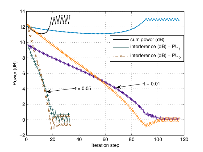
In Figs. 6 and 7, we consider a SU MIMO-BC network with K=5K=5, Nt=5N_{t}=5, Nr=3N_{r}=3, and Pu=13P_{u}=13 dB. In this example, the SUs with w1=5w_{1}=5 and wi=1,i=2,…,Kw_{i}=1,~i=2,\ldots,K are assumed to share the same spectrum band with two PUs. Fig. 6 plots the weighted sum rate versus the number of iterations of the SIPA algorithm for step sizes t=0.1t=0.1 and t=0.01t=0.01. As can be seen from the figure, the step size affects the accuracy and convergence speed of the algorithm. Fig. 7 plots the sum power at the BS and the interference power at the PUs versus the number of iterations. It can be seen from the figure that the sum power and the interference power approach to Pu=13P_{u}=13 dB and Pt=0P_{t}=0 dB respectively when the SIPA algorithm converges. This implies that the sum power and interference constraints are satisfied with equalities when the SIPA algorithm converges.

Example 4

Fig. 8 plots the achievable sum rates versus the sum power in the single PU case and the case with no PU. We choose K=5K=5, Nt=5N_{t}=5, and Nr=3N_{r}=3. As can be seen from Fig. 8, in the low sum power regime, the achievable sum rate in the case with no PU is quite close to the one in the single PU case while in the high sum power regime, the achievable sum rate in the case with no PU is much higher than the one in the single PU case. This is because the additional constraint reduces the degrees of freedom of the system.

Example 5

In this example, we consider the influence of the interference constraint on the achievable sum rate of the SUs. In this example, Nt=5N_{t}=5, K=5K=5, and Nr=3N_{r}=3. The sum power constraint for the BS is assumed to be 15 dB and 20 dB. Fig. 9 compares the sum rate achieved in a PU case with one achieved in the case with no PU as l2/l1l_{2}/l_{1} varies from 1 to 12. It can be observed from the figure that the achievable sum rate increases as the PU moves away from the BS, and the influence of the PU reduces to zero after the l2/l1l_{2}/l_{1} is larger than a certain threshold.

VII Conclusions

In this paper, we developed a new BC-MAC duality result, which can be viewed as an extension of existing dual results developed under either a sum power constraint or per-antenna power constraints. Exploiting this duality result, we proposed an efficient algorithm to solve the CR MIMO-BC weighted sum rate maximization problem. We further showed that the proposed algorithm converges to the globally optimal solution.

A Lemma 4 and its proof

The following lemma describes an important property that will be used in the proof of other lemmas.

Lemma 4

For fixed qtq_{t} and quq_{u}, the maximum weighted sum rate in (5) is achieved when the constraint (6) is satisfied with equality.

Proof:

We here adopt the DPC scheme, which is a capacity achieving strategy for the MIMO-BC [16]. Let the permutation π\pi represent the encoding order when the optimal solution is achieved. Assume that SUπ(1) is encoded first such that the signal of SUπ(1) is noncausally known to the BS before the signals from the other SUs are encoded. Thus, in the DPC scheme the signal from SUπ(1) has no impact on the rates achieved by the other SUs. We prove this lemma by contradiction.

Suppose that 𝑸π⁡(1)b{\mbox{\boldmath$Q$}}^{\text{b}}_{\pi(1)} is the optimal signal covariance matrix of SUπ(1). Assume that the constraint (6) is satisfied with a strict inequality when the optimal solution is achieved. Thus, we can always find an ϵ>0\epsilon>0 such that

qt​(∑i=2K𝒉o†​(𝑸π⁡(i)b)​𝒉o+𝒉o†​(𝑸π⁡(1)b+ϵ​𝑰)​𝒉o−Pt)+qu​(∑i=2Ktr​(𝑸π⁡(i)b)+tr​(𝑸π⁡(1)b+ϵ​𝑰)−Pu)\displaystyle q_{t}\big(\sum_{i=2}^{K}{\mbox{\boldmath$h$}}_{o}^{{\dagger}}({\mbox{\boldmath$Q$}}^{\text{b}}_{\pi(i)}){\mbox{\boldmath$h$}}_{o}+{\mbox{\boldmath$h$}}_{o}^{{\dagger}}({\mbox{\boldmath$Q$}}^{\text{b}}_{\pi(1)}+\epsilon{\mbox{\boldmath$I$}}){\mbox{\boldmath$h$}}_{o}-P_{t}\big)+q_{u}\big(\sum_{i=2}^{K}\text{tr}({\mbox{\boldmath$Q$}}^{\text{b}}_{\pi(i)})+\text{tr}({\mbox{\boldmath$Q$}}^{\text{b}}_{\pi(1)}+\epsilon{\mbox{\boldmath$I$}})-P_{u}\big)
=qt​(∑i=1K𝒉o†​(𝑸π⁡(i)b)​𝒉o+𝒉o†​(ϵ​𝑰)​𝒉o−Pt)+qu​(∑i=1Ktr​(𝑸π⁡(i)b)+tr​(ϵ​𝑰)−Pu)<0.\displaystyle=q_{t}\big(\sum_{i=1}^{K}{\mbox{\boldmath$h$}}_{o}^{{\dagger}}({\mbox{\boldmath$Q$}}^{\text{b}}_{\pi(i)}){\mbox{\boldmath$h$}}_{o}+{\mbox{\boldmath$h$}}_{o}^{{\dagger}}(\epsilon{\mbox{\boldmath$I$}}){\mbox{\boldmath$h$}}_{o}-P_{t}\big)+q_{u}\big(\sum_{i=1}^{K}\text{tr}({\mbox{\boldmath$Q$}}^{\text{b}}_{\pi(i)})+\text{tr}(\epsilon{\mbox{\boldmath$I$}})-P_{u}\big)<0. (43)

Moreover, the rate achieved by user π⁡(1)\pi(1) in the MIMO-BC can be written as

rπ⁡(1)b=log⁡|𝑰+∑i=1K𝑯π⁡(1)​𝑸π⁡(i)b​𝑯π⁡(1)†||𝑰+∑i=2K𝑯π⁡(1)​𝑸π⁡(i)b​𝑯π⁡(1)†|.r_{\pi(1)}^{\text{b}}=\log\frac{\Big|{\mbox{\boldmath$I$}}+\sum_{i=1}^{K}{\mbox{\boldmath$H$}}_{\pi(1)}{\mbox{\boldmath$Q$}}_{\pi(i)}^{\text{b}}{\mbox{\boldmath$H$}}_{\pi(1)}^{{\dagger}}\Big|}{\Big|{\mbox{\boldmath$I$}}+\sum_{i=2}^{K}{\mbox{\boldmath$H$}}_{\pi(1)}{\mbox{\boldmath$Q$}}_{\pi(i)}^{\text{b}}{\mbox{\boldmath$H$}}_{\pi(1)}^{{\dagger}}\Big|}.

Due to the positive semi-definiteness property of 𝑸ib{\mbox{\boldmath$Q$}}_{i}^{\text{b}}, we have

log⁡|𝑰+∑i=2K𝑯π⁡(1)​𝑸π⁡(i)b​𝑯π⁡(1)†+𝑯π⁡(1)​(𝑸π⁡(1)b+ϵ​𝑰)​𝑯π⁡(1)†|\displaystyle\log\Big|{\mbox{\boldmath$I$}}+\sum_{i=2}^{K}{\mbox{\boldmath$H$}}_{\pi(1)}{\mbox{\boldmath$Q$}}^{\text{b}}_{\pi(i)}{\mbox{\boldmath$H$}}_{\pi(1)}^{{\dagger}}+{\mbox{\boldmath$H$}}_{\pi(1)}({\mbox{\boldmath$Q$}}^{\text{b}}_{\pi(1)}+\epsilon{\mbox{\boldmath$I$}}){\mbox{\boldmath$H$}}_{\pi(1)}^{{\dagger}}\Big|
=\displaystyle= log⁡|𝑰+∑i=2K𝑯π⁡(1)​𝑸π⁡(i)b​𝑯π⁡(1)†|\displaystyle\log\Big|{\mbox{\boldmath$I$}}+\sum_{i=2}^{K}{\mbox{\boldmath$H$}}_{\pi(1)}{\mbox{\boldmath$Q$}}^{\text{b}}_{\pi(i)}{\mbox{\boldmath$H$}}_{\pi(1)}^{{\dagger}}\Big|
+\displaystyle+ log|𝑰+(𝑰+∑i=2K𝑯π⁡(1)𝑸π⁡(i)b𝑯π⁡(1)†)−1/2𝑯π⁡(1)(𝑸π⁡(1)b+ϵ𝑰)𝑯π⁡(1)†(𝑰+∑i=2K𝑯π⁡(1)𝑸π⁡(i)b𝑯π⁡(1)†)−1/2|\displaystyle\log\Big|{\mbox{\boldmath$I$}}\!\!+({\mbox{\boldmath$I$}}\!+\sum_{i=2}^{K}{\mbox{\boldmath$H$}}_{\pi(1)}{\mbox{\boldmath$Q$}}^{\text{b}}_{\pi(i)}{\mbox{\boldmath$H$}}_{\pi(1)}^{{\dagger}})^{-1/2}{\mbox{\boldmath$H$}}_{\pi(1)}({\mbox{\boldmath$Q$}}^{\text{b}}_{\pi(1)}\!\!+\epsilon{\mbox{\boldmath$I$}}){\mbox{\boldmath$H$}}_{\pi(1)}^{{\dagger}}({\mbox{\boldmath$I$}}\!+\sum_{i=2}^{K}{\mbox{\boldmath$H$}}_{\pi(1)}{\mbox{\boldmath$Q$}}^{\text{b}}_{\pi(i)}{\mbox{\boldmath$H$}}_{\pi(1)}^{{\dagger}})^{-1/2}\Big|
=\displaystyle= log⁡|𝑰+∑i=2K𝑯π⁡(1)​𝑸π⁡(i)b​𝑯π⁡(1)†|+log⁡|𝑰+𝑮†​(𝑸π⁡(1)b+ϵ​𝑰)​𝑮|\displaystyle\log\Big|{\mbox{\boldmath$I$}}+\sum_{i=2}^{K}{\mbox{\boldmath$H$}}_{\pi(1)}{\mbox{\boldmath$Q$}}^{\text{b}}_{\pi(i)}{\mbox{\boldmath$H$}}_{\pi(1)}^{{\dagger}}\Big|+\log\Big|{\mbox{\boldmath$I$}}+{\mbox{\boldmath$G$}}^{{\dagger}}({\mbox{\boldmath$Q$}}^{\text{b}}_{\pi(1)}+\epsilon{\mbox{\boldmath$I$}}){\mbox{\boldmath$G$}}\Big|
=\displaystyle= log⁡|𝑰+∑i=2K𝑯π⁡(1)​𝑸π⁡(i)b​𝑯π⁡(1)†|+log⁡|𝑰+𝚲+ϵ​𝚺|\displaystyle\log\Big|{\mbox{\boldmath$I$}}+\sum_{i=2}^{K}{\mbox{\boldmath$H$}}_{\pi(1)}{\mbox{\boldmath$Q$}}^{\text{b}}_{\pi(i)}{\mbox{\boldmath$H$}}_{\pi(1)}^{{\dagger}}\Big|+\log\Big|{\mbox{\boldmath$I$}}+{\bf\Lambda}+\epsilon{\bf\Sigma}\Big| (44)
>\displaystyle> log⁡|𝑰+∑i=2K𝑯π⁡(1)​𝑸π⁡(i)b​𝑯π⁡(1)†|+log⁡|𝑰+𝚲|\displaystyle\log\Big|{\mbox{\boldmath$I$}}+\sum_{i=2}^{K}{\mbox{\boldmath$H$}}_{\pi(1)}{\mbox{\boldmath$Q$}}^{\text{b}}_{\pi(i)}{\mbox{\boldmath$H$}}_{\pi(1)}^{{\dagger}}\Big|+\log\Big|{\mbox{\boldmath$I$}}+{\bf\Lambda}\Big|
=\displaystyle= log⁡|𝑰+∑i=1K𝑯π⁡(1)​𝑸π⁡(i)b​𝑯π⁡(1)†|,\displaystyle\log\Big|{\mbox{\boldmath$I$}}+\sum_{i=1}^{K}{\mbox{\boldmath$H$}}_{\pi(1)}{\mbox{\boldmath$Q$}}^{\text{b}}_{\pi(i)}{\mbox{\boldmath$H$}}_{\pi(1)}^{{\dagger}}\Big|, (45)

where 𝑮=𝑯π⁡(1)†(𝑰+∑i=2K𝑯π⁡(1)𝑸π⁡(i)b𝑯π⁡(1)†)−1/2{\mbox{\boldmath$G$}}={\mbox{\boldmath$H$}}_{\pi(1)}^{{\dagger}}({\mbox{\boldmath$I$}}+\sum_{i=2}^{K}{\mbox{\boldmath$H$}}_{\pi(1)}{\mbox{\boldmath$Q$}}^{\text{b}}_{\pi(i)}{\mbox{\boldmath$H$}}_{\pi(1)}^{{\dagger}})^{-1/2}, and 𝚲{\bf\Lambda} and 𝚺{\bf\Sigma} are diagonal matrices. Eq. (44) is due to the fact that the optimal covariance matrix for a MIMO has the water-filling structure [19][24], i.e., if we apply singular value decomposition to 𝑮G, 𝑮=𝑽𝑺𝑼{\mbox{\boldmath$G$}}={\mbox{\boldmath$V$}}{\mbox{\boldmath$S$}}{\mbox{\boldmath$U$}}, where 𝑽V and 𝑼U are unitary matrices, and 𝑺S is a diagonal matrix, then the optimal 𝑸π⁡(1)b{\mbox{\boldmath$Q$}}^{\text{b}}_{\pi(1)} can be written as 𝑸π⁡(1)b=𝑼†​𝑹𝑼{\mbox{\boldmath$Q$}}^{\text{b}}_{\pi(1)}={\mbox{\boldmath$U$}}^{{\dagger}}{\mbox{\boldmath$R$}}{\mbox{\boldmath$U$}}, where 𝑹R is a diagonal matrix. Thus, we have 𝚲=𝑺𝑹𝑺\bf\Lambda={\mbox{\boldmath$S$}}{\mbox{\boldmath$R$}}{\mbox{\boldmath$S$}} and 𝚺=𝑺𝑺\bf\Sigma={\mbox{\boldmath$S$}}{\mbox{\boldmath$S$}}.

According to (45) and (43), 𝑸π⁡(1)b+ϵ​𝑰{\mbox{\boldmath$Q$}}^{\text{b}}_{\pi(1)}+\epsilon{\mbox{\boldmath$I$}} is a better solution for the sum rate problem than 𝑸π⁡(1)b{\mbox{\boldmath$Q$}}^{\text{b}}_{\pi(1)}, which contradicts with the assumption. Therefore, the constraint must be satisfied with equality. ∎

B Proof of Proposition 1

The proof consists of two parts. In the first part, we show that either optimal solution is feasible for both problems. In the second part, we show that Problem 1 and Problem 2 have the same solution.

The Lagrangian function of Problem 1 is

L1​(𝑸1b,⋯,𝑸Kb,λt,λu)=∑i=1Kwi​rib−λt​(∑i=1K𝒉o†​𝑸ib​𝒉o−Pt)−λu​(∑i=1Ktr​(𝑸ib)−Pu),L_{1}({\mbox{\boldmath$Q$}}^{\text{b}}_{1},\cdots,{\mbox{\boldmath$Q$}}^{\text{b}}_{K},\lambda_{t},\lambda_{u})=\sum_{i=1}^{K}w_{i}r_{i}^{\text{b}}-\lambda_{t}\big(\sum_{i=1}^{K}{\mbox{\boldmath$h$}}_{o}^{{\dagger}}{\mbox{\boldmath$Q$}}_{i}^{\text{b}}{\mbox{\boldmath$h$}}_{o}-P_{t}\big)-\lambda_{u}\big(\sum_{i=1}^{K}\text{tr}({\mbox{\boldmath$Q$}}_{i}^{\text{b}})-P_{u}\big), (46)

where λt\lambda_{t} and λu\lambda_{u} are the Lagrangian multipliers. The optimal objective value is

minλt,λu​max𝑸1b,⋯,𝑸Kb​L1​(𝑸1b,⋯,𝑸Kb,λt,λu).\underset{\lambda_{t},\lambda_{u}}{\text{min}}\underset{{\mbox{\small\boldmath$Q$}}^{\text{b}}_{1},\cdots,{\mbox{\small\boldmath$Q$}}^{\text{b}}_{K}}{\text{max}}L_{1}({\mbox{\boldmath$Q$}}^{\text{b}}_{1},\cdots,{\mbox{\boldmath$Q$}}^{\text{b}}_{K},\lambda_{t},\lambda_{u}). (47)

Assume the optimal variables are λ¯t\bar{\lambda}_{t}, λ¯u\bar{\lambda}_{u} and 𝑸¯1b,⋯,𝑸¯Kb\bar{{\mbox{\boldmath$Q$}}}^{\text{b}}_{1},\cdots,\bar{{\mbox{\boldmath$Q$}}}^{\text{b}}_{K}, and the corresponding optimal value is C¯\bar{C}.

The Lagrangian function of Problem 2 is:

L2​(𝑸1b,⋯,𝑸Kb,qt,qu,λ)=∑iwi​rib−λ⁡(qt​(∑i=1K𝒉o†​𝑸ib​𝒉o−Pt)+qu​(∑i=1Ktr​(𝑸ib)−Pu)),L_{2}({\mbox{\boldmath$Q$}}^{\text{b}}_{1},\cdots,{\mbox{\boldmath$Q$}}^{\text{b}}_{K},q_{t},q_{u},\lambda)=\sum_{i}w_{i}r_{i}^{\text{b}}-\lambda\Big(q_{t}\big(\sum_{i=1}^{K}{\mbox{\boldmath$h$}}_{o}^{{\dagger}}{\mbox{\boldmath$Q$}}_{i}^{\text{b}}{\mbox{\boldmath$h$}}_{o}-P_{t}\big)+q_{u}\big(\sum_{i=1}^{K}\text{tr}({\mbox{\boldmath$Q$}}_{i}^{\text{b}})-P_{u}\big)\Big), (48)

where λ\lambda is the Lagrangian multiplier. The optimal objective value is

minqt,qu,λ​max𝑸1b,⋯,𝑸Kb​L2​(𝑸1b,⋯,𝑸Kb,qt,qu,λ).\underset{q_{t},q_{u},\lambda}{\text{min}}\underset{{\mbox{\small\boldmath$Q$}}^{\text{b}}_{1},\cdots,{\mbox{\small\boldmath$Q$}}^{\text{b}}_{K}}{\text{max}}L_{2}({\mbox{\boldmath$Q$}}^{\text{b}}_{1},\cdots,{\mbox{\boldmath$Q$}}^{\text{b}}_{K},q_{t},q_{u},\lambda). (49)

Suppose that the optimal variables are q~t\tilde{q}_{t}, q~u\tilde{q}_{u}, λ~\tilde{\lambda}, and 𝑸~ib,i=1,…,K\tilde{{\mbox{\boldmath$Q$}}}^{\text{b}}_{i}~,i=1,\ldots,K, and the corresponding optimal objective value is C~\tilde{C}. We just need to prove C¯=C~\bar{C}=\tilde{C}.

We now present the first part of the proof. According to the KKT condition of Problem 2, we have

∂L2​(λ~,𝑸~1b,⋯,𝑸~Kb,q~t,q~u)∂qt=λ~​(∑i=1K𝒉o†​𝑸~ib​𝒉o−Pt)=0,\displaystyle\frac{\partial L_{2}(\tilde{\lambda},\tilde{{\mbox{\boldmath$Q$}}}^{\text{b}}_{1},\cdots,\tilde{{\mbox{\boldmath$Q$}}}^{\text{b}}_{K},\tilde{q}_{t},\tilde{q}_{u})}{\partial q_{t}}=\tilde{\lambda}\big(\sum_{i=1}^{K}{\mbox{\boldmath$h$}}_{o}^{{\dagger}}\tilde{{\mbox{\boldmath$Q$}}}_{i}^{\text{b}}{\mbox{\boldmath$h$}}_{o}-P_{t}\big)=0, (50)
∂L2​(λ~,𝑸~1b,⋯,𝑸~Kb,q~t,q~u)∂qu=λ~​(∑i=1Ktr​(𝑸~ib)−Pu)=0.\displaystyle\frac{\partial L_{2}(\tilde{\lambda},\tilde{{\mbox{\boldmath$Q$}}}^{\text{b}}_{1},\cdots,\tilde{{\mbox{\boldmath$Q$}}}^{\text{b}}_{K},\tilde{q}_{t},\tilde{q}_{u})}{\partial q_{u}}=\tilde{\lambda}\big(\sum_{i=1}^{K}\text{tr}(\tilde{{\mbox{\boldmath$Q$}}}_{i}^{\text{b}})-P_{u}\big)=0. (51)

Recall that the Lagrangian multiplier λ~\tilde{\lambda} is non-negative. Furthermore, if λ~=0\tilde{\lambda}=0, we have q~t​(∑i=1K𝒉o†​𝑸~i​𝒉o−Pt)+q~u​(∑i=1Ktr​(𝑸~i)−Pu)<0\tilde{q}_{t}(\sum_{i=1}^{K}{\mbox{\boldmath$h$}}_{o}^{{\dagger}}\tilde{{\mbox{\boldmath$Q$}}}_{i}{\mbox{\boldmath$h$}}_{o}-P_{t})+\tilde{q}_{u}(\sum_{i=1}^{K}\text{tr}(\tilde{{\mbox{\boldmath$Q$}}}_{i})-P_{u})<0 from the KKT conditions. This contradicts with Lemma 4. Thus, we always have λ~>0\tilde{\lambda}>0 and can readily conclude that ∑i=1K𝒉o†​𝑸~ib​𝒉o=Pt\sum_{i=1}^{K}{\mbox{\boldmath$h$}}_{o}^{{\dagger}}\tilde{{\mbox{\boldmath$Q$}}}_{i}^{\text{b}}{\mbox{\boldmath$h$}}_{o}=P_{t} and ∑i=1Ktr​(𝑸~ib)=Pu\sum_{i=1}^{K}\text{tr}(\tilde{{\mbox{\boldmath$Q$}}}_{i}^{\text{b}})=P_{u} are satisfied simultaneously. The optimal solution of Problem 2 is also a feasible solution of Problem 1. On the other hand, it is obvious that the feasible solution for Problem 1 is also the feasible solution for Problem 2.

We next prove the second part by using contradiction. Let us first suppose C¯>C~\bar{C}>\tilde{C}. For (48), if we select 𝑸ib=𝑸¯ib{\mbox{\boldmath$Q$}}^{\text{b}}_{i}=\bar{{\mbox{\boldmath$Q$}}}^{\text{b}}_{i} for i=1,…,Ki=1,\ldots,K, λ=1\lambda=1, qt=λ¯tq_{t}=\bar{\lambda}_{t} and qu=λ¯uq_{u}=\bar{\lambda}_{u}, then L2=C¯>C~L_{2}=\bar{C}>\tilde{C}. It contradicts to the fact that C~\tilde{C} is the optimal objective value for (49).

We now assume C¯<C~\bar{C}<\tilde{C}. Recall that λ~≠0\tilde{\lambda}\neq 0, for (48). If we select 𝑸ib=𝑸~ib{\mbox{\boldmath$Q$}}^{\text{b}}_{i}=\tilde{{\mbox{\boldmath$Q$}}}^{\text{b}}_{i} for i=1,…,Ki=1,\ldots,K, λt=λ~​qt~\lambda_{t}=\tilde{\lambda}\tilde{q_{t}} and λu=λ~​q~u\lambda_{u}=\tilde{\lambda}\tilde{q}_{u}, then L1=C~>C¯L_{1}=\tilde{C}>\bar{C}, which contradicts with the fact that C¯\bar{C} is the optimal objective value for (47).

Therefore, the optimal solutions for Problem 2 and Problem 1 are the same. ■\blacksquare

C Proof of Lemma 1

According to previous discussions, the signal from each SU is divided into several data streams. We now show that the optimal encoding order of these data streams are arbitrary. It is well known that the optimal objective value of the MAC equally weighted sum rate problem can be achieved by adopting any ordering [19][17][18]; that is, when all the users have the same weights, the optimal solution of the weighted sum rate maximization problem is independent of the decoding order. Analogously, the data streams within a SU share the same weight. Thus, an arbitrary encoding order of those data streams within a SU can achieve the optimal solution. ■\blacksquare

D Proof of Lemma 2

Let ss be the sub-gradient of g⁡(λ~)g(\tilde{\lambda}). For a given λ~≥0\tilde{\lambda}\geq 0, the subgradient ss of g⁡(λ~)g(\tilde{\lambda}) satisfies g⁡(λˇ)≥g⁡(λ~)+s⁡(λˇ−λ~)g(\check{\lambda})\geq g(\tilde{\lambda})+s(\check{\lambda}-\tilde{\lambda}), where λˇ\check{\lambda} is any feasible value. Let 𝑸ˇim,i=1,…,K\check{{\mbox{\boldmath$Q$}}}^{\text{m}}_{i},~i=1,\ldots,K, be the optimal covariance matrices in (27) for λ=λˇ\lambda=\check{\lambda}, and 𝑸~im,i=1,…,K\tilde{{\mbox{\boldmath$Q$}}}^{\text{m}}_{i},~i=1,\ldots,K, be the optimal covariance matrices in (27) for λ=λ~\lambda=\tilde{\lambda}. We express g⁡(λˇ)g(\check{\lambda}) as

g⁡(λˇ)\displaystyle g(\check{\lambda}) =max𝑸1m,⋯,𝑸Km​(f⁡(𝑸1m,⋯,𝑸Km)−λˇ​(∑i=1Ktr​(𝑸im)−P))\displaystyle=\underset{{\mbox{\small\boldmath$Q$}}^{\text{m}}_{1},\cdots,{\mbox{\small\boldmath$Q$}}^{\text{m}}_{K}}{\text{max}}\Big(f({\mbox{\boldmath$Q$}}^{\text{m}}_{1},\cdots,{\mbox{\boldmath$Q$}}^{\text{m}}_{K})-\check{\lambda}(\sum_{i=1}^{K}\text{tr}({\mbox{\boldmath$Q$}}_{i}^{\text{m}})-P)\Big)
=f⁡(𝑸ˇ1m,⋯,𝑸ˇKm)−λˇ​(∑i=1Ktr​(𝑸ˇim)−P)\displaystyle=f(\check{{\mbox{\boldmath$Q$}}}^{\text{m}}_{1},\cdots,\check{{\mbox{\boldmath$Q$}}}^{\text{m}}_{K})-\check{\lambda}\Big(\sum_{i=1}^{K}\text{tr}(\check{{\mbox{\boldmath$Q$}}}^{\text{m}}_{i})-P\Big)
≥f⁡(𝑸~1m,⋯,𝑸~Km)−λˇ​(∑i=1Ktr​(𝑸~im)−P)\displaystyle\geq f(\tilde{{\mbox{\boldmath$Q$}}}^{\text{m}}_{1},\cdots,\tilde{{\mbox{\boldmath$Q$}}}^{\text{m}}_{K})-\check{\lambda}\Big(\sum_{i=1}^{K}\text{tr}(\tilde{{\mbox{\boldmath$Q$}}}_{i}^{\text{m}})-P\Big)
=f⁡(𝑸~1m,⋯,𝑸~Km)−λ~​(∑i=1Ktr​(𝑸~im)−P)+λ~​(∑i=1Ktr​(𝑸~im)−P)−λˇ​(∑i=1Ktr​(𝑸~im)−P)\displaystyle=f(\tilde{{\mbox{\boldmath$Q$}}}^{\text{m}}_{1},\cdots,\tilde{{\mbox{\boldmath$Q$}}}^{\text{m}}_{K})\!-\!\tilde{\lambda}\Big(\sum_{i=1}^{K}\text{tr}(\tilde{{\mbox{\boldmath$Q$}}}_{i}^{\text{m}})\!\!-\!P\Big)\!\!+\!\tilde{\lambda}\Big(\sum_{i=1}^{K}\text{tr}(\tilde{{\mbox{\boldmath$Q$}}}_{i}^{\text{m}})\!-\!P\Big)\!-\!\check{\lambda}\Big(\sum_{i=1}^{K}\text{tr}(\tilde{{\mbox{\boldmath$Q$}}}_{i}^{\text{m}})-P\Big)
=g⁡(λ~)+(P−∑i=1Ktr​(𝑸~im))​(λˇ−λ~),\displaystyle=g(\tilde{\lambda})+\Big(P-\sum_{i=1}^{K}\text{tr}(\tilde{{\mbox{\boldmath$Q$}}}_{i}^{\text{m}})\Big)(\check{\lambda}-\tilde{\lambda}),

where s:=P−∑i=1Ktr​(𝑸~im)s:=P-\sum_{i=1}^{K}\text{tr}(\tilde{{\mbox{\boldmath$Q$}}}_{i}^{\text{m}}) is the subgradient of g⁡(λ~)g(\tilde{\lambda}). This concludes the proof. ■\blacksquare

E Proof of Lemma 3

The subgradient 𝒔s of g⁡(q~t,q~u)g(\tilde{q}_{t},\tilde{q}_{u}) satisfies g⁡(q¯t,q¯u)≥g⁡(q~t,q~u)+([q¯t,q¯u]−[q~t,q~u])⋅𝒔Tg(\bar{q}_{t},\bar{q}_{u})\geq g(\tilde{q}_{t},\tilde{q}_{u})+([\bar{q}_{t},\bar{q}_{u}]-[\tilde{q}_{t},\tilde{q}_{u}])\cdot{\mbox{\boldmath$s$}}^{T}, where [q¯t,q¯u][\bar{q}_{t},\bar{q}_{u}] is any feasible vector. Let 𝑸¯ib​i=1,…,K,\bar{{\mbox{\boldmath$Q$}}}_{i}^{\text{b}}~i=1,\ldots,K, be the optimal matrices of the problem (33) for qt=q¯tq_{t}=\bar{q}_{t} and qu=q¯uq_{u}=\bar{q}_{u}, and let 𝑸~ib​i=1,…,K,\tilde{{\mbox{\boldmath$Q$}}}_{i}^{\text{b}}~i=1,\ldots,K, be the optimal matrices of the problem (33) for qt=q~tq_{t}=\tilde{q}_{t} and qu=q~uq_{u}=\tilde{q}_{u}. We express g⁡(q¯t,q¯u)g(\bar{q}_{t},\bar{q}_{u}) as

g⁡(q¯t,q¯u)=max𝑸1b,⋯,𝑸Kb​∑i=1Mwi​rib\displaystyle g(\bar{q}_{t},\bar{q}_{u})\!=\underset{{\mbox{\small\boldmath$Q$}}^{\text{b}}_{1},\cdots,{\mbox{\small\boldmath$Q$}}^{\text{b}}_{K}}{\text{max}}\!\sum_{i=1}^{M}w_{i}r_{i}^{\text{b}} (52)
=\displaystyle= ∑i=1Mwi​r¯ib−λ¯​(q¯t​(∑i=1K𝒉o†​𝑸b¯i​𝒉o−Pt)+q¯u​(∑i=1Ktr​(𝑸b¯i)−Pu))\displaystyle\!\sum_{i=1}^{M}w_{i}\bar{r}_{i}^{\text{b}}\!-\!\bar{\lambda}\big(\bar{q}_{t}\big(\sum_{i=1}^{K}{\mbox{\boldmath$h$}}_{o}^{{\dagger}}\bar{{\mbox{\boldmath$Q$}}^{\text{b}}}_{i}{\mbox{\boldmath$h$}}_{o}-P_{t}\big)+\bar{q}_{u}\big(\sum_{i=1}^{K}\text{tr}(\bar{{\mbox{\boldmath$Q$}}^{\text{b}}}_{i})-P_{u}\big)\big) (53)
≥\displaystyle\geq ∑i=1Mwi​r~ib−λ¯​(q¯t​(∑i=1K𝒉o†​𝑸~ib​𝒉o−Pt)+q¯u​(∑i=1Ktr​(𝑸~ib)−Pu))\displaystyle\sum_{i=1}^{M}w_{i}\tilde{r}_{i}^{\text{b}}-\bar{\lambda}\Big(\bar{q}_{t}\big(\sum_{i=1}^{K}{\mbox{\boldmath$h$}}_{o}^{{\dagger}}\tilde{{\mbox{\boldmath$Q$}}}_{i}^{\text{b}}{\mbox{\boldmath$h$}}_{o}-P_{t}\big)+\bar{q}_{u}\big(\sum_{i=1}^{K}\text{tr}(\tilde{{\mbox{\boldmath$Q$}}}_{i}^{\text{b}})-P_{u}\big)\Big) (54)
=\displaystyle= ∑i=1Mwi​r~ib−λ~​(q~t​(∑i=1K𝒉o†​𝑸~ib​𝒉o−Pt)+q~u​(∑i=1Ktr​(𝑸~ib)−Pu))\displaystyle\sum_{i=1}^{M}w_{i}\tilde{r}_{i}^{\text{b}}-\tilde{\lambda}\Big(\tilde{q}_{t}\big(\sum_{i=1}^{K}{\mbox{\boldmath$h$}}_{o}^{{\dagger}}\tilde{{\mbox{\boldmath$Q$}}}_{i}^{\text{b}}{\mbox{\boldmath$h$}}_{o}-P_{t}\big)+\tilde{q}_{u}\big(\sum_{i=1}^{K}\text{tr}(\tilde{{\mbox{\boldmath$Q$}}}_{i}^{\text{b}})-P_{u}\big)\Big)
+λ~​(q~t​(∑i=1K𝒉o†​𝑸~ib​𝒉o−Pt)+q~u​(∑i=1Ktr​(𝑸~ib)−Pu))−λ¯​(q¯t​(∑i=1K𝒉o†​𝑸~ib​𝒉o−Pt)+q¯u​(∑i=1Ktr​(𝑸~ib)−Pu))\displaystyle+\tilde{\lambda}\!\Big(\!\tilde{q}_{t}\big(\!\sum_{i=1}^{K}{\mbox{\boldmath$h$}}_{o}^{{\dagger}}\tilde{{\mbox{\boldmath$Q$}}}_{i}^{\text{b}}{\mbox{\boldmath$h$}}_{o}\!\!-\!\!P_{t}\big)\!\!+\!\!\tilde{q}_{u}\big(\!\sum_{i=1}^{K}\text{tr}(\tilde{{\mbox{\boldmath$Q$}}}_{i}^{\text{b}})\!\!-\!\!P_{u}\big)\!\Big)\!-\!\bar{\lambda}\!\Big(\!\bar{q}_{t}\big(\!\sum_{i=1}^{K}{\mbox{\boldmath$h$}}_{o}^{{\dagger}}\tilde{{\mbox{\boldmath$Q$}}}_{i}^{\text{b}}{\mbox{\boldmath$h$}}_{o}\!\!-\!\!P_{t}\big)\!\!+\!\!\bar{q}_{u}\big(\!\sum_{i=1}^{K}\text{tr}(\tilde{{\mbox{\boldmath$Q$}}}_{i}^{\text{b}})\!\!-\!\!P_{u}\big)\!\Big)
=\displaystyle= g⁡(q~t,q~u)+(∑i=1K𝒉o†​𝑸~ib​𝒉o−Pt)​(λ~​q~t−λ¯​q¯t)+(∑i=1Ktr​(𝑸~ib)−Pu)​(λ~​q~u−λ¯​q¯u)\displaystyle g(\tilde{q}_{t},\tilde{q}_{u})+\Big(\sum_{i=1}^{K}{\mbox{\boldmath$h$}}_{o}^{{\dagger}}\tilde{{\mbox{\boldmath$Q$}}}_{i}^{\text{b}}{\mbox{\boldmath$h$}}_{o}-P_{t}\Big)(\tilde{\lambda}\tilde{q}_{t}-\bar{\lambda}\bar{q}_{t})+\Big(\sum_{i=1}^{K}\text{tr}(\tilde{{\mbox{\boldmath$Q$}}}_{i}^{\text{b}})-P_{u}\Big)(\tilde{\lambda}\tilde{q}_{u}-\bar{\lambda}\bar{q}_{u})
=\displaystyle= g⁡(q~t,q~u)+(∑i=1K𝒉o†​𝑸~ib​𝒉o−Pt)​(λ~​q~t−λ¯​q~t+λ¯​q~t−λ¯​q¯t)\displaystyle g(\tilde{q}_{t},\tilde{q}_{u})+\Big(\sum_{i=1}^{K}{\mbox{\boldmath$h$}}_{o}^{{\dagger}}\tilde{{\mbox{\boldmath$Q$}}}_{i}^{\text{b}}{\mbox{\boldmath$h$}}_{o}-P_{t}\Big)(\tilde{\lambda}\tilde{q}_{t}-\bar{\lambda}\tilde{q}_{t}+\bar{\lambda}\tilde{q}_{t}-\bar{\lambda}\bar{q}_{t})
+(∑i=1Ktr​(𝑸~ib)−Pu)​(λ~​q~u−λ¯​q~u+λ¯​q~u−λ¯​q¯u)\displaystyle+\Big(\sum_{i=1}^{K}\text{tr}(\tilde{{\mbox{\boldmath$Q$}}}_{i}^{\text{b}})-P_{u}\Big)(\tilde{\lambda}\tilde{q}_{u}-\bar{\lambda}\tilde{q}_{u}+\bar{\lambda}\tilde{q}_{u}-\bar{\lambda}\bar{q}_{u})
=\displaystyle= g⁡(q~t,q~u)+(∑i=1K𝒉o†​𝑸~ib​𝒉o−Pt)​(λ~​q~t−λ¯​q~t)+(∑i=1K𝒉o†​𝑸~ib​𝒉o−Pt)​(λ¯​q~t−λ¯​q¯t)\displaystyle g(\tilde{q}_{t},\tilde{q}_{u})+\Big(\sum_{i=1}^{K}{\mbox{\boldmath$h$}}_{o}^{{\dagger}}\tilde{{\mbox{\boldmath$Q$}}}_{i}^{\text{b}}{\mbox{\boldmath$h$}}_{o}-P_{t}\Big)(\tilde{\lambda}\tilde{q}_{t}-\bar{\lambda}\tilde{q}_{t})+\Big(\sum_{i=1}^{K}{\mbox{\boldmath$h$}}_{o}^{{\dagger}}\tilde{{\mbox{\boldmath$Q$}}}_{i}^{\text{b}}{\mbox{\boldmath$h$}}_{o}-P_{t}\Big)(\bar{\lambda}\tilde{q}_{t}-\bar{\lambda}\bar{q}_{t})
+(∑itr​(𝑸~ib)−Pu)​(λ~​q~u−λ¯​q~u)+(∑i=1Ktr​(𝑸~ib)−Pu)​(λ¯​q~u−λ¯​q¯u)\displaystyle+\Big(\sum_{i}\text{tr}(\tilde{{\mbox{\boldmath$Q$}}}_{i}^{\text{b}})-P_{u}\Big)(\tilde{\lambda}\tilde{q}_{u}-\bar{\lambda}\tilde{q}_{u})+\Big(\sum_{i=1}^{K}\text{tr}(\tilde{{\mbox{\boldmath$Q$}}}_{i}^{\text{b}})-P_{u}\Big)(\bar{\lambda}\tilde{q}_{u}-\bar{\lambda}\bar{q}_{u})
=\displaystyle= g⁡(q~t,q~u)+(∑i=1K𝒉o†​𝑸~ib​𝒉o−Pt)​(λ¯​q~t−λ¯​q¯t)+(∑i=1Ktr​(𝑸~ib)−Pu)​(λ¯​q~u−λ¯​q¯u)\displaystyle g(\tilde{q}_{t},\tilde{q}_{u})+\Big(\sum_{i=1}^{K}{\mbox{\boldmath$h$}}_{o}^{{\dagger}}\tilde{{\mbox{\boldmath$Q$}}}_{i}^{\text{b}}{\mbox{\boldmath$h$}}_{o}-P_{t}\Big)(\bar{\lambda}\tilde{q}_{t}-\bar{\lambda}\bar{q}_{t})+\Big(\sum_{i=1}^{K}\text{tr}(\tilde{{\mbox{\boldmath$Q$}}}_{i}^{\text{b}})-P_{u}\Big)(\bar{\lambda}\tilde{q}_{u}-\bar{\lambda}\bar{q}_{u}) (55)
=\displaystyle= g⁡(qt,qu)+λ¯​([q¯t,q¯u]−[q~t,q~u])⋅𝒔T,\displaystyle g(q_{t},q_{u})+\bar{\lambda}([\bar{q}_{t},\bar{q}_{u}]-[\tilde{q}_{t},\tilde{q}_{u}])\cdot{\mbox{\boldmath$s$}}^{T},

where 𝒔:=[Pt−∑i=1K𝒉o†​𝑸~ib​𝒉o,Pu−∑i=1Ktr​(𝑸~ib)]{\mbox{\boldmath$s$}}:=[P_{t}-\sum_{i=1}^{K}{\mbox{\boldmath$h$}}_{o}^{{\dagger}}\tilde{{\mbox{\boldmath$Q$}}}_{i}^{\text{b}}{\mbox{\boldmath$h$}}_{o},P_{u}-\sum_{i=1}^{K}\text{tr}(\tilde{{\mbox{\boldmath$Q$}}}_{i}^{\text{b}})]. Eq. (53) is due to the fact that the dual objective function of the problem (33), and r¯ib\bar{r}_{i}^{\text{b}}, λ¯\bar{\lambda}, and 𝑸¯ib\bar{{\mbox{\boldmath$Q$}}}_{i}^{\text{b}} are the optimal variables for the fixed q¯t\bar{q}_{t} and q¯u\bar{q}_{u}. The inequality (54) is because 𝑸¯ib,i=1,…,K\bar{{\mbox{\boldmath$Q$}}}_{i}^{\text{b}}~,i=1,\ldots,K, are the optimal signal covariance matrices for the fixed q¯t\bar{q}_{t} and q¯u\bar{q}_{u}. The equality (55) is due to Lemma 4. Thus, 𝒔s is the subgradient of g⁡(q~t,q~u)g(\tilde{q}_{t},\tilde{q}_{u}). ■\blacksquare

References

  • [1] F. C. Commission, “Facilitating opportunities for flexible, efficient, and reliable spectrum use employing cognitive radio technologies, notice of proposed rule making and order, fcc 03-322,” Dec. 2003.
  • [2] J. Mitola and G. Q. Maguire, “Cognitive radios: Making software radios more personal,” IEEE Personal Communications, vol. 6, no. 4, pp. 13–18, Aug. 1999.
  • [3] S. Haykin, “Cognitive radio: Brain-empowered wireless communications,” IEEE J. Select. Areas Commun., vol. 23, no. 2, pp. 201–202, Feb. 2005.
  • [4] Y. Xing, C. Mathur, M. Haleem, R. Chandramouli, and K. Subbalakshmi, “Dynamic spectrum access with QoS and interference temperature constraints,” IEEE Trans. Mobile Comput., vol. 6, no. 4, pp. 423–433, Apr. 2007.
  • [5] M. Gastpar, “On capacity under receive and spatial spectrum-sharing constraints,” IEEE Trans. Inform. Theory, vol. 53, no. 2, pp. 471–487, Feb. 2007.
  • [6] A. Ghasemi and E. S. Sousa, “Fundamental limits of spectrum-sharing in fading environments,” IEEE Trans. Wireless Commun., vol. 6, no. 2, pp. 649–658, Feb. 2007.
  • [7] Y.-C. Liang, Y. Zeng, E. Peh, and A. Hoang, “Sensing-throughput tradeoff for cognitive radio networks,” IEEE Trans. Wireless Commun., vol. 7, no. 4, pp. 1326–1337, Apr. 2008.
  • [8] M. Kobayashi and G. Caire, “An iterative water-filling algorithm for maximum weighted sum-rate of Gaussian MIMO-BC,” IEEE J. Select. Areas Commun., vol. 24, no. 8, pp. 1640–1646, Aug. 2006.
  • [9] L. Jia and T. Hou, “Maximum weighted sum rate of multi-antenna broadcast channels,” 2007. [Online]. Available: http://arXiv:cs/0703111v1.
  • [10] F. Rashid-Farrokhi, L. Tassiulas, and K. Liu, “Joint optimal power control and beamforming in wireless networks using antenna arrays,” IEEE Trans. Commun., vol. 46, no. 10, pp. 1313–1324, Oct. 1998.
  • [11] P. Viswanath and D. N. C. Tse, “Sum capacity of the vector Gaussian broadcast channel and uplink-downlink duality,” IEEE Trans. Inform. Theory, vol. 49, no. 8, pp. 1912–1921, Aug. 2003.
  • [12] S. Vishwanath, N. Jindal, and A. Goldsmith, “Duality, achievable rates, and sum-rate capacity of Gaussian MIMO broadcast channels,” IEEE Trans. Inform. Theory, vol. 49, no. 10, pp. 2658–2668, Oct. 2003.
  • [13] Z.-Q. Luo and W. Yu, “An introduction to convex optimization for communications and signal processing,” IEEE J. Select. Areas Commun., vol. 24, no. 8, pp. 1426–1438, Aug. 2006.
  • [14] D. Tse and S. Hanly, “Multiaccess fading channels-part I: Polymatriod structure, optimal resource allocation and throughtput capacities,” IEEE Trans. Inform. Theory, vol. 44, no. 7, pp. 2796–2815, Nov. 1998.
  • [15] W. Yu and J. Cioffi, “Sum capacity of Gaussian vector broadcast channels,” IEEE Transactions on information theory, vol. 50, pp. 1875–1892, Sept. 2004.
  • [16] H. Weingarten, Y. Steinberg, and S. Shamai, “The capacity region of the Gaussian multiple-input multiple-output broadcast channel,” IEEE Trans. Inform. Theory, vol. 52, no. 9, pp. 3936–64, Sept. 2006.
  • [17] N. Jindal, W. Rhee, S. Vishwanath, S. A. Jafar, and A. Goldsmith, “Sum power iterative water-filling for multi-antenna Gaussian broadcast channels,” IEEE Trans. Inform. Theory, vol. 51, no. 4, pp. 1570–1580, Apr. 2005.
  • [18] W. Yu, “Sum-capacity computation for the Gaussian vector broadcast channel via dual decomposition,” IEEE Trans. Inform. Theory, vol. 52, no. 2, pp. 754–759, Feb. 2006.
  • [19] W. Yu, W. Rhee, S. Boyd, and J. M. Cioffi, “Iterative water-filling for Gaussian vector multiple-access channels,” IEEE Trans. Inform. Theory, vol. 50, no. 1, pp. 145–152, Jan. 2004.
  • [20] W. Yu and T. Lan, “Transmitter optimization for the multi-antenna downlink with per-antenna power constraints,” IEEE Trans. Signal Processing, vol. 55, no. 6, pp. 2646–2660, June 2007.
  • [21] D. G. Luenberger, Optimization by vector space methods. New York: John Wiley, 1969.
  • [22] A. Wiesel, Y. C. Eldar, and S. Shamai, “Linear precoding via conic optimization for fixed MIMO receivers,” IEEE Trans. Signal Processing, vol. 54, no. 1, pp. 161–176, Jan. 2006.
  • [23] S. Boyd and L. Vandenberghe, Convex Optimization. Cambridge, UK: Cambridge University Press, 2004.
  • [24] I. E. Telatar, “Capacity of multi-antenna Gaussian channels,” European Trans. on Telecomm., vol. 10, no. 6, pp. 585–595, Oct. 1999.
  • [25] S. Boyd, L. Xiao, and A. Mutapcic, “Subgradient methods,” 2003. [Online]. Available: http://mit.edu/6.976/www/notes/subgrad_method.pdf.
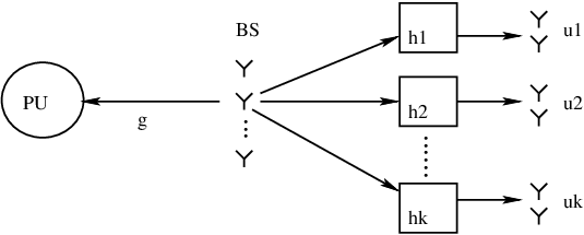
Refer to caption
Fig. 1: The system model for MIMO-BC based cognitive radio networks. There are KK SUs. The BS of the SUs has NtN_{t} transmit antennas, and each SU is equipped with NrN_{r} receive antennas.
Refer to caption

BC, 𝒛i∼𝒩⁡(0,σ2​𝑰Nr){\mbox{\boldmath$z$}}_{i}\sim\mathcal{N}(0,\sigma^{2}{\mbox{\boldmath$I$}}_{N_{r}}),

qt​∑i=1K𝒉o†​𝑸ib​𝒉o+qu​∑i=1Ktr​(𝑸ib)≤Pq_{t}\sum_{i=1}^{K}{\mbox{\boldmath$h$}}_{o}^{{\dagger}}{\mbox{\boldmath$Q$}}_{i}^{\text{b}}{\mbox{\boldmath$h$}}_{o}+q_{u}\sum_{i=1}^{K}\text{tr}({\mbox{\boldmath$Q$}}_{i}^{\text{b}})\leq P

Refer to caption

Dual MAC, 𝒛∼𝒩⁡(0,qt​𝑹o+qu​𝑰Nt){\mbox{\boldmath$z$}}\sim\mathcal{N}(0,q_{t}{\mbox{\boldmath$R$}}_{o}+q_{u}{\mbox{\boldmath$I$}}_{N_{t}}),

∑i=1Ktr​(𝑸im)​σ2≤P,𝑹o=𝒉o​𝒉oH\sum_{i=1}^{K}\text{tr}({\mbox{\boldmath$Q$}}_{i}^{\text{m}})\sigma^{2}\leq P,~{\mbox{\boldmath$R$}}_{o}={\mbox{\boldmath$h$}}_{o}{\mbox{\boldmath$h$}}_{o}^{H}

Fig. 2: The system models for Problem 3 and Problem 4, where qtq_{t} and quq_{u} are constant, and 𝑹o=𝒉o​𝒉o†{\mbox{\boldmath$R$}}_{o}={\mbox{\boldmath$h$}}_{o}{\mbox{\boldmath$h$}}_{o}^{{\dagger}}.
Refer to caption
Fig. 3: The flow chart for the SIPA algorithm, where 𝑸i,(n)b{\mbox{\boldmath$Q$}}_{i,(n)}^{\text{b}} and 𝑸i,(n)n{\mbox{\boldmath$Q$}}_{i,(n)}^{\text{n}} denote the transmit signal covariance matrices of SUi for the BC and MAC at the nnth step, respectively.
Refer to caption
Fig. 4: Comparison of the optimal achievable rates obtained by the DIPA and the water-filling algorithm in a MIMO channel (Nt=Nr=4N_{t}=N_{r}=4, K=1K=1 and PuP_{u}=10 dB).
Refer to caption
Fig. 5: Convergence behavior of the DIPA algorithm (K=20K=20 and Pu=10P_{u}=10 dB).
Refer to caption
Fig. 6: Convergence behavior of the SIPA algorithm (Nt=5N_{t}=5, K=5K=5, Nr=3N_{r}=3, w1=5w_{1}=5, and wi=1w_{i}=1, for i≠1i\neq 1).
Refer to caption
Fig. 7: The convergence behavior of the sum power at the BS and the interference at the PU for the SIPA algorithm (Nt=5N_{t}=5, K=5K=5, Nr=3N_{r}=3, w1=5w_{1}=5, and wi=1w_{i}=1 with i≠1i\neq 1).
Refer to caption
Fig. 8: Achievable sum rates versus sum power in the single PU case and the case with no PU (Nt=5N_{t}=5, K=5K=5, Nr=3N_{r}=3).
Refer to caption
Fig. 9: Achievable sum rates versus the ratio of l2/l1l_{2}/l_{1} using the SIPA algorithm (Nt=5N_{t}=5, K=5K=5, Nr=3N_{r}=3).