There is a long history to Chiral Symmetry Breaking. It began with CVC and the Goldberger-Treiman relation [1], and proceeded through the ground-breaking work of Gell-Mann and Lévy who invented PCAC and the linear and non-linear $\sigma$ models [2]. Their Lagrangian began from chiral symmetry in the sense that both $\pi$ and $\sigma$ fields appear on an equal footing, but the symmetry between them is spontaneously broken by introducing a negative $\phi^{4}$ term.

Adler [3] showed that in both $\pi N$ and $\pi\pi$ systems there is a zero at the unphysical point $t=m_{\pi}^{2}$ midway between the thresholds of $s$ and $u$ channels. ‘Soft’ pion theory, current algebra and QCD led to the Standard Model. With the idea that ‘bare’ quarks are almost massless, Gasser and Leutwyler introduced Chiral Perturbation Theory as a systematic method of expanding amplitudes in the domain where pion masses and momenta are small [4].

The S-wave elastic scattering amplitude may be written

where $\rho$ is the usual phase space factor. The numerator $N(s)$ is real and describes ‘driving forces’ from the left-hand cut. Unitarity is accomodated by means of the $K$-matrix. The Adler zero in the $\pi\pi$ amplitude makes the S-wave unusual. When one projects out the S-wave from the full amplitude, there is a zero at $s=s_{A}\simeq m_{\pi}^{2}/2$. The amplitude near the $\pi\pi$ threshold rises nearly linearly. The simplest acceptable form is [5]

where $b$, $M$ and $\gamma$ are constants; the exponential makes $K\to 0$ as $s\to\infty$ but introduces non-linearity in a controlled way. Above the $KK$ threshold

A similar approach has been used by Pelaez, Oset and Oller [6] [7] in a series of papers building Chiral Symmetry Breaking into fits to data. During the era 1975 to 1995, many theorists fitted the $\pi\pi$ S-wave in ways similar to this and found a pole with mass roughly 500 MeV and a large width $\sim$ 500 MeV.

In elastic scattering, the Adler zero in the numerator makes the amplitude small near the $\pi\pi$ threshold. However, in a production process, the numerator need not contain the Adler zero, and is in fact consistent within rather small errors with a constant. The $\sigma$ pole appeared clearly in E791 data on $D^{+}\to\pi^{-}\pi^{+}\pi^{+}$ [8] and BES data on $J/\Psi\to\omega\pi^{+}\pi^{-}$ [9]. Both sets of data show a conspicuous peak visible by eye at $\sim 500$ MeV. Fig. 1 shows the Dalitz plot and mass projections for BES data. There are conspicuous diagonal bands due to the $\sigma$ and $f_{2}(1270)$ and vertical/horizontal bands due to $b_{1}(1235)\to\omega\pi$. The $\pi\pi$ mass projection is shown in (b) and the $\sigma$ component in (d). Those data may be fitted simultaneously with elastic scattering data; BES found a pole at $541\pm 39-i(252\pm 42)$ MeV.

Since 2004, couplings to $KK$ and $\eta\eta$ have been determined by fitting (a) all available data on $\pi\pi\to KK$ and $\eta\eta$, (b) Kloe and Novosibirsk data on $\phi\to\gamma(\pi^{0}\pi^{0})$ [10]. All these data agree on a substantial coupling of $\sigma$ to $KK$. A further refinement is to include in the Breit-Wigner denominator a dispersive correction $m(s)$ (discussed below). The $\sigma$ pole moves to $500\pm 30-i(264\pm 30)$ MeV.

There was some debate whether the peak could be due to interference with a ‘background’. However, BES data give a phase variation with $s$ consistent with elastic scattering and hence a simple pole [11]. Secondly, Caprini et al. calculated a prediction from the Roy equations and driving forces on the left-hand cut [12]. The great merit of this calculation is that it maps out the magnitude and phase of the S-wave amplitude over the whole of the low mass region of the complex $s$-plane, including the sub-threshold region inaccessible to experiment. This leaves no possible doubt of the existence of the pole and gives a pole position $M=441^{+16}_{-8}-i(272^{+9}_{-12.5})$ MeV. However, the result for $D(s)$ does not reproduce accurately the upper side of the $\sigma$ peak in BES data. A combined fit to their predictions and BES data using $(b_{1}+b_{2}s)$ instead of $b$ in Eq. (2) gives $M=472\pm 30-i(271\pm 30)$ MeV without departing from their predicted phases by more than $1.5^{\circ}$ [13].

Understanding the $\sigma$ pole requires some gymnastics in complex variables. It lies at $s=0.15-i0.26$ GeV², not too far above the $\pi\pi$ threshold but far into the complex plane. The phase shift is $90^{\circ}$ just above the pole. But on the real $s$-axis where experiments are done, the phase shift must go to 0 at the $\pi\pi$ threshold. There is therefore a strong variation of the phase as one moves into the complex plane. This arises directly from the Cauchy-Riemann equations: the Adler zero gives a real part of the amplitude rising nearly linearly with $s$ at low mass, and there must be a corresponding variation of the imaginary part of the amplitude with ${\rm Im}\,s$. Roughly speaking, the pole would give rise to a phase shift approaching $150^{\circ}$ at 1 GeV, but the effect of unitarity is to distort the phase observed on the real $s$-axis to $90^{\circ}$ at 1 GeV. For the $\kappa$, the effect is even larger. The $\kappa$ pole lies almost below the $K\pi$ threshold and is very broad. The consequence is that the phase shift measured on the real $s$ axis only reaches $70^{\circ}$ at 1400 MeV/c.

At the Hadron95 conference, Mike Scadron asked me if there could be a $\kappa$ resonance below 1 GeV. At the time, the only reply which could be given was that it must be very broad if it exists at all. Later, Zheng and collaborators [14] showed that including the Adler zero in the fit to LASS phase shifts for $K\pi$ elastic scattering and including the effects of unitarity and analyticity demands a pole at $M=694\pm 53$ MeV, $\Gamma=606\pm 59$ MeV. Descotes-Genon and Moussallam obtained a pole at $M=658\pm 13$ MeV, $\Gamma=557\pm 24$ MeV [15] using the Roy equations.

A low mass peak appears in E791 data on $D^{+}\to K^{-}\pi^{+}\pi^{+}$ [16] and BES data on $J/\Psi\to K^{+}\pi^{-}K^{-}\pi^{+}$ [17]. Experimentalists have been bewildered by the strange behaviour of the $K\pi$ phase shift and have undertaken the task of determining the magnitude and phase of the $S$-wave amplitude in bins of mass up to 1700 MeV/c [18]. It turns out that these E791 results, the BES data and LASS phase shifts may all be fitted simultaneously [19] with $M=750^{+30}_{-55}-i(342\pm 60)$ MeV. This result is rather higher in mass than the prediction from the Roy equations, but again much of the discrepancy can be traced to the effect of the strong $K\eta^{\prime}$ threshold, which was not included in the treatment of the Roy equations.

The way the fit to data goes is as follows. The LASS data [20] play a strong role in determining the phase of the amplitude. The BES data determine the parameters of the strong $K_{0}(1430)$ observed there - considerably stronger than in LASS or E791 data. The E791 data determine the magnitude of the amplitude, which turns out to be accurately consistent with the phase variation when the numerator of the production amplitude is taken to be constant. This is a clear example how one can improve the precision of the analysis by fitting several sets of data simultaneously.

Currently, the Belle, Babar and CLEO C collaborations make fits without the Adler zero. Fits including it are urgently needed to reduce the confusion. Are they claiming their results demonstrate that Chiral Symmetry is not broken in the $K\pi$ sector? That seems unlikely in view of the fact that the Adler zero is very well established in the heavier $\pi N$ sector.

The whole question of how resonances can be attracted to thresholds is discussed in a full length article [21] and will be recapitulated here. In the Breit-Wigner denominator of a resonance, there must be dispersive terms in the real part

In fact, the terms $ig^{2}_{i}\rho_{i}$ of Eq. (3) arise from the pole at $s^{\prime}=s$ in Eq. (4).

Fig. 2 shows $m_{KK}(s)$ and $g^{2}_{KK}\rho_{KK}(s)$ near the $KK$ threshold, using a form factor $e^{-3k^{2}}$, where $k$ is centre of mass $KK$ momentum in GeV/c. There is a cusp in $m_{KK}(s)$ at the threshold. It is positive definite at the theshold, signifying additional attraction there.

If the cusp is superimposed on attraction from another source, for example meson exchanges, a resonance can be generated by the peak in $m_{KK}(s)$. The locking of $a_{0}(980)$ and $f_{0}(980)$ to the $KK$ threshold is explained naturally by this cusp mechanism.

Near threshold, the wave function of the resonance has a long tail, like the deuteron. This tail is purely mesonic; contributions from coloured quarks are confined in the resonance at short range or in the decay mesons. Confined quarks have kinetic energy $k^{2}/2m=-(\hbar^{2}/2m)\nabla^{2}\Psi$; here $k$ and $m$ are quark momentum and effective mass and $\Psi$ is the wave function. To create a bound state, extra potential energy must compensate the kinetic energy of the confined particles. This again pulls the resonance towards the threshold. Törnqvist provides a formula allowing an estimate of the meson-meson component [22]; for the $f_{0}(980)$ it is at least $60\%$ and for $a_{0}(980)$ at least $\sim 35\%$.

Other examples of resonances appearing at sharp thresholds are known: $f_{2}(1565)$ at the $\omega\omega$ threshold, $K_{0}(1430)$ at the $K\eta^{\prime}$ threshold, $\Lambda_{C}(2940)$ at the $D^{0}p$ threshold, and $X(3872)$ at the $\bar{D}(1865)D^{*}(2007)$ threshold.

The nonet of $\sigma$, $\kappa$, $a_{0}(980)$ and $f_{0}(980)$ may be understood quantitatively in terms of meson exchanges, witness the calculations from the Roy equations by Caprini et al. and Descotes-Genon et al. Janssen et al. have shown that the $f_{0}(980)$ may be fitted well in terms of $K^{*}$ and $\rho$ exchanges in $u$ and $t$ channels [23]. However, most mesons and baryons are explained as quark-model states. There has been much debate about ‘molecules’ and multi-quark states, e.g. $qq\bar{q}\bar{q}$.

One of the mysteries of the quark model is how confined states penetrate the confining potential and turn into mesons. How, for example, does the $\rho$ ‘know’ to have the right width to create the $\sigma$ pole via the Roy equations? My suggestion is that the confining potential arises as a cooperative effect between QCD at short range (coloured quarks and gluons) and meson exchanges at long range. Meson exchanges are certainly present, witness the peaks observed at small $t$ and $u$. If both QCD and meson exchanges contribute, the well known eigenvalue equation is

where $H_{11}$ and $H_{22}$ describe isolated $\bar{q}q$ and meson-meson configurations and $V$ describes mixing. This mixing pushes the eigenstate down in mass. This is the well known Variational Principle which minimises the eigenvalue when states mix. It is closely analogous to formation of a covalent bond in chemistry.

Van Beveren and Rupp [24] have proposed a similar idea. They adopt a transition potential which couples states confined in a harmonic oscillator potential to outgoing waves; they match the logarithmic derivative at a $\delta$ function transition radius $\sim 0.65$ fm, though they mention the possibility of a gradual transition with a ${}^{3}P_{0}$ dependence on radius. The $\sigma$, $\kappa$, $a_{0}(980)$ and $f_{0}(980)$ emerge from the continuum when the coupling constant to confined states increases. The simplicity of their model makes it easy to follow the movement of poles as this coupling constant is varied. They illustrated results for the $\kappa$ and $a_{o}(980)$ poles. The dependence of the $\sigma$, $\kappa$, $a_{0}(980)$ and $f_{0}(980)$ poles on the coupling constant is tabulated in Ref. [25]. The model reproduces well the amplitudes for all these states using a universal coupling constant and SU3 Clebsch-Gordan coefficients. The $a_{0}$ does not appear at the $\eta\pi$ threshold because of its associated Adler zero. If the coupling constant is increased by a factor 2.5, the $\sigma$, $\kappa$ and $a_{0}$ all become bound states.

There has been great enthusiasm for explaining states observed in charmonium physics as 4-quark states. However, Valcarce et al. [26] find from a detailed model calculation that such states always appear higher in mass than $c\bar{c}$ configurations with the same quantum numbers, unless attractive interactions arise between diquarks. At short range, coloured combinations could contribute to a lowering of the energy of the $c\bar{c}n\bar{n}$ eigenstate. However, the long-range tail of such an eigenstate is uncoloured, taking us back to a meson-meson configuration.

Molecular states certainly exist as nuclei. The nucleon-nucleon interaction is a classic example of meson exchanges. There is a repulsive core due to the Pauli principle pushing identical quarks apart.

Oset, Oller and collaborators find that they can account for many resonances from a chiral Lagrangian [27] [28]. This is essentially a meson-meson interaction with Chiral Symmetry Breaking built in. They also include short-range $q\bar{q}$ interactions. However, the short-range interactions need to be tuned to reproduce accurately the masses, widths and branching ratios of $f_{0}(1370/1310)$, $f_{0}(1500)$, $f_{0}(1710)$ and $f_{0}(1790)$. In the $\pi N$ system, Donnachie and Hamilton showed in 1965 that meson exchanges are attractive for quantum numbers where there are prominent resonances: $P_{33}(1232)$, $D_{13}(1520)$, $D_{15}(1675)$, $F_{15}(1680$, etc. [29].

Ochs has waged a long campaign claiming that Cern-Munich (CM) data [30] are better than the sum total of all other data and disprove the existence of $f_{0}(1370)$ . This is not true. CM data give an excellent determination of $\pi\pi$ phase shifts $\delta$ from 610 MeV to the $KK$ threshold (990 MeV). However, above this there are strong correlations between $\delta$ and elasticity parameters $\eta$; consequently, errors on both become large. These are illustrated in Figs. 4 and 6 of Au, Morgan and Pennington [31] and in Fig. 1 of Kaminski, Pelaez and Yndurain [32]; errors for $\eta$ are very large because of lack of data determining accurately the absolute magnitudes of $\pi\pi\to KK$, $\eta\eta$ and particularly the dominant channel $4\pi$.

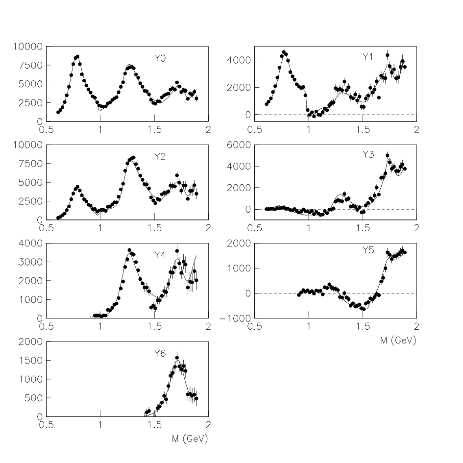
It is easy to check these errors directly from errors on CM moments. For every bin, four algebraic solutions emerge. There is some constraint on the $\pi\pi$ D-wave from the line-shape of $f_{2}(1270)$. However, there is a substantial contribution from $f_{2}(1565)$, ignored by Ochs. It couples strongly to $\omega\omega$ [33]; the sub-threshold continuation of this channel is poorly known, as is its coupling to $\rho\rho$. Consequently, there is large uncertainty in the D-wave contribution to moments $Y_{4}$, $Y_{2}$ and $Y_{0}$. Also the $\rho(1450)$ and $\rho(1700)$ cannot be identified in CM data, leading to further poorly identified contributions to $Y_{2}$, $Y_{1}$ and $Y_{0}$. All these systematic uncertainties accumulate in $Y_{0}$, which determines the S-wave intensity; it can be fitted very flexibly. Fig. 3 shows my fit to CM moments using fully analytic functions (a major constraint). Some mixing is required (and expected) between $f_{0}(1370)$, $\sigma$ and $f_{0}(1500)$, which overlap strongly. Mixing induces a phase rotation of the $f_{0}(1370)$, see [34].

The problem in identifying $f_{0}(1370)$ is that its $2\pi$ decay is obscured in many sets of data by $f_{2}(1270)$. However, it produces a clearly visible peak in $\bar{p}p\to\eta\eta\pi^{0}$ at rest; this peak cannot be due to $f_{2}(1270)$ which has a branching fraction to $\eta\eta$ of only 0.4%. It is also visible as a peak in BES data for $J/\Psi\to\phi\pi^{+}\pi^{-}$ [35], where angular correlations between production and decay of the $\phi$ separate $J^{P}=0^{+}$ and $2^{+}$ cleanly. It was first observed in 3 sets of data on $\pi\pi\to KK$ from ANL and BNL [36] [37] [38]. Its parameters are best determined by Crystal Barrel data on $\bar{p}p\to 3\pi^{0}$ at rest in liquid and gaseous hydrogen; these data separate ${}^{1}S_{0}$ and ${}^{3}P_{1}$ annihilation, which give independent determinations of mass and width agreeing within $\pm 5$ and $\pm 10$ MeV respectively. Crystal Barrel data on charge combinations of $\bar{p}p\to KK\pi$ give consistent parameters with all other data [39].

The resonance mass is $1309\pm 15$ MeV with a full-width at half maximum of $207\pm 15$ MeV. However, the rapid opening of the $4\pi$ threshold moves the peak in $4\pi$ higher by $\sim 80$ MeV because of phase space. The opening of the $4\pi$ channel was not taken into account in most analyses, leading to confusion and inflated errors. The $f_{0}(1370)$ was observed by Gasparo [40] and then by Crystal Barrel, Obelix and WA102 in many sets of $4\pi$ data [41]. When one allows for $4\pi$ phase space and the associated dispersive effect, all observations where both $f_{0}(1310/1370)$ and $f_{0}(1500)$ have been fitted are close to consistency within errors.

With the $f_{0}(1370)$, $f_{0}(1500)$ and $f_{0}(1710)$ well established, there is one state too many to fit as $\bar{n}n$ and $s\bar{s}$. The glueball predicted in this mass range by Lattice Gauge calculations mixes with the $q\bar{q}$ states. The $f_{0}(1710)$ decays almost purely to $KK$, with a possible small $\eta\eta$ decay. The $f_{0}(1500)$ behaves as an octet state with $\Gamma(\eta\eta)/\Gamma(\pi\pi)=0.145\pm 0.027$ and $\Gamma(K\bar{K})/\Gamma(\pi\pi)=0.246\pm 0.026$.

An intriguing result is the sharp $\omega\phi$ signal reported by the BES collaboration [42], peaking at 1812 MeV, just above the $\phi\omega$ threshold at 1801 MeV. A purely threshold effect should peak much higher. It is therefore probably due to $f_{0}(1790)$, a resonance clearly separated from $f_{0}(1710)$ in BES data on $J/\Psi\to\omega KK$ [43], $\omega\pi\pi$ [9], $\phi\pi\pi$ and $\phi KK$ [35]. There is a strong $f_{0}(1710)$ peak in $\omega KK$ data, but nothing in $\omega\pi\pi$ despite large statistics. Conversely, the $f_{0}(1790)$ appears clearly in $\phi\pi\pi$, but not in $\phi KK$. There is a factor 22 difference in decay branching ratios to $\pi\pi$ and $KK$, requiring separate $f_{0}(1710)$ and $f_{0}(1790)$. The $f_{0}(1790)$ was first observed in $J/\Psi\to\gamma 4\pi$ [44] [45]. It makes a natural radial excitation of $f_{0}(1370)$.

The $\phi\omega$ decay can arise naturally from a glueball component in $f_{0}(1790)$ [46]. A glueball is a flavour singlet with flavour content

[The $s\bar{s}$ component might be enhanced with respect to $n\bar{n}$ by a factor $f^{2}_{K}/f^{2}_{\pi}=1.21$.] The component $2(u\bar{u}+d\bar{d})s\bar{s}$ can make $4\omega\phi$ or $2(K^{*0}\bar{K}^{*0}+K^{*+}K^{*-})$ or a linear combination. BES I data on $J/\Psi\to\gamma(K^{+}\pi^{-}K^{-}\pi^{+})$ show that the $\gamma(K^{*}\bar{K}^{*})$ channel contains no significant $0^{+}$ signal [47]. A signal with the same magnitude as that of $J/\Psi\to\gamma(\omega\phi)$ would be conspicuous near 1800 MeV. Its absence may be qualitatively explained by the larger phase space for $(u\bar{u}+d\bar{d})s\bar{s}$ in $KK$ decays than in $K^{*}\bar{K}^{*}$.

In fitting $\sigma$ and $\kappa$, it is essential to include the Adler zero explicitly into the Breit-Wigner denominator - or demonstrate that such a fit is unacceptably bad. The Adler zero needs to be included also into the $K_{0}(1430)$. It would be good if competing experimental groups would join forces, like LEP groups, to try and achieve an optimum compromise between different sets of data and iron out inconsistencies. Experience is that different sets of data illuminate different aspects required for an optimum fit.

The $\sigma$, $\kappa$, $a_{0}(980)$ and $f_{0}(980)$ fit naturally according to meson exchanges. Why look further? The cusp at the $KK$ threshold plays an essential role in locking $a_{0}$ and $f_{0}$ to this threshold. The cusp mechanism can attract a resonance over a surprisingly large mass interval of $\sim\pm 100$ MeV. At the threshold, zero point energy is minimised by the long-range tail of the wave function. Mixing between quark configurations and meson-meson states minimises the energy of the linear combination in a way analogous to the formation of a covalent bond in chemistry. This idea is similar to the idea of Duality between resonances and particle exchanges.

I wish to thank Prof. G. Rupp and Prof. E. van Beveren for extensive discussions and for their efforts in organising a workshop on Scalar Mesons to mark the 70th birthday of Mike Scadron. I am very grateful to Mike Scadron for illuminating the role of PCAC and the linear $\sigma$ model on many occasions.

References

- [1] M.L. Goldberger and S.B. Treiman, Phys. Rev. 109 (1958) 193
- [2] M. Gell-Mann and M. Lévy, Nu. Cim. 16 (1960) 1729
- [3] S.L. Adler , Phys. Rev. 137 B (1965) 1022
- [4] J. Gasser and H. Leutwyler, Phys. Lett. B 125 (1983) 616
- [5] D.V. Bugg, Phys. Lett. B 572 (2003) 1
- [6] A.Dobado and J.R.Pelaez, Phys. Rev. D 47 (1993) 4883
- [7] J.A. Oller, E.Oset and J.R. Pelaez, Phys. Rev. D59 (1999) 074001
- [8] E.M. Aitala et al., Phys. Rev. Lett. 86 (2001) 770
- [9] M. Ablikim et al., Phys. Lett. B598 (2004) 149
- [10] D.V. Bugg, Eur. Phys. J C 47 (2006) 45
- [11] D.V. Bugg, Eur. Phys. J C37 (2004) 433
- [12] I. Caprini, I. Colangelo and H. Leutwyler, Phys. Rev. Lett. 96 (2006) 032001
- [13] D.V. Bugg, J. Phys. G 34 (2007) 151
- [14] Z.Y Zhou and H.Q. Zheng, Nucl. Phys. A (2006) 212
- [15] S. Descotes-Genon and B. Moussallam, Eur. Phys. J C48 (2006) 553
- [16] E.M. Aitala et al., Phys. Rev. Lett. 89 (2002) 121801
- [17] M. Ablikim et al., Phys. Lett. B633 (2006) 681
- [18] E.M.Aitala et al., Phys. Rev. D73 (2006) 032004
- [19] D.V. Bugg, Phys. Lett. B 632 (2006) 471
- [20] D. Aston et al., Nucl. Phys. B296 (1988) 493
- [21] D.V. Bugg, arXiv: hep-ph/0802.0934
- [22] N.A. Törnqvist, Z. Phys. C68 (1995) 647.
- [23] G. Janssen et al., Phys. Rev. D52 (1995) 2690
- [24] E. van Beveren and G. Rupp, AIP Conf, Proc. 660 (2003) 353.
- [25] E. van Beveren et al., Phys. Lett. B461 (2006) 265
- [26] A. Vakcarce, J. Vijande and N. Barnea, arXiv: hep-ph/0711.3114
- [27] D. Gamermann et al., hep-ph/0710.5365
- [28] M. Albaladejo, J.A. Oller and C. Piqueras, hep-ph/0711.1977
- [29] A. Donnachie and J. Hamilton, Phys. Rev. 138 (1965) B678
- [30] B.D. Hyams et al., Nucl. Phys. B 54 (1973) 134
- [31] K.L. Au, D. Morgan and M.R. Pennington, Phys. Rev. D35 (1987) 1633
- [32] R. Kaminski, J.R. Pelaez and F.J. Yndurain, Phys. Rev. D74 (2006) 014001
- [33] C.A. Baker et al., Phys. Lett. B467 (1999) 147
- [34] D.V. Bugg, Euro. Phys. J C52 (2007) 55
- [35] M. Ablikim et al. (BES Collaboration), Phys. Lett. B607 (2005) 243
- [36] D. Cohen et al., Phys. Rev. D22 (1980) 2595
- [37] V.A. Polychronakos et al., Phys. Rev. D19 (1979) 1317
- [38] A. Etkin et al., Phys. Rev. D25 (1982) 1786
- [39] V.V. Anisovich and A.V. Sarantsev, Eur. Phys. J. A16 (2003) 229
- [40] M. Gaspero, Nucl. Phys. A562 (2003) 407
- [41] Particle Data Group, J. Phys. G33 (2006) 1.
- [42] M. Ablikim et al. (BES Collaboration), Phys. Rev. Lett. 96 (2006) 162002
- [43] M. Ablikim et al. (BES Collaboration), Phys. Lett. B603 (2004) 138
- [44] D.V. Bugg et al., Phys. Lett. B353 (1995) 378
- [45] J.Z. Bai et al (BES Collaboration) Phys. Lett. B472 (2000) 207
- [46] P. Bicudo et al., arXiv: hep-ph/0602172
- [47] J. Z. Bai et al., Phys. Lett. B472 (2000) 200