LOW ENERGY PION-PION ELASTIC SCATTERING IN SAKAI-SUGIMOTO MODEL
R.Parthasarathy 11 1 e-mail address:sarathy@cmi.ac.in
Chennai Mathematical Institute
Plot.H1, SIPCOT IT Park, Padur Post
Siruseri 603103, India.
and
K.S.Viswanathan22 2 e-mail address:kviswana@sfu.ca
Department of Physics and IRMACS
Simon Fraser University
Burnaby, Canada V5A1S6.
Abstract
We have considered the holographic large QCD model proposed by Sakai and Sugimoto and evaluated the non-Abelian DBI-action on the -brane upto terms. Restricting to the pion sector, these corrections give rise to four derivative contact terms for the pion field. We derive the Weinberg’s phenemenological lagragian. The coefficients of the four derivative terms are determined in terms of . The low energy pion-pion scattering amplitudes are evaluated. Numerical results are presented with the choice of and . The results are compared with the amplitudes calculated using the experimental phase shifts. The agreement with the experimental data is found to be satisfactory.
PACS Classification: 11.25.-w; 11.25.Uv
I.Introduction
A study of pion-pion scattering is one of the methods to investigate the nature of the strong interactions. The standard approach at low energies is the use of the chiral perturbation theory, which enables one to calculate the scattering amplitudes near threshold [1]. The pion physics at low energies is described by the effective chiral lagrangian,
| (1) |
where , is the pion field, , is the pion decay constant and . Weinberg [2] obtained the pion-pion scattering amplitude from (1) as
| (2) |
where are the Mandelstam variables satisfying .
The real scattering amplitudes of definite isospin are given by
| (3) |
where,
is the pion momentum in the center of mass frame and is the scattering angle. The partial wave isospin amplitudes are given by
| (4) |
with . The current-algebra result (2) gives rising almost linearly with thereby violating the unitarity bound, namely, even below 1GeV. Dispersion theoretic study by Roy [3] gave the result for the above amplitudes consistent with the unitarity bound. However, the various parameters involved are to be determined by the experimental data.
Weinberg [1], in his phenemenological approach, suggested adding two more terms to (1) involving four pion field (four derivative contact terms) with arbitrary coefficients as
| (5) | |||||
where and are dimensionless constants and is given by (1). The effect of the additional terms in (5) on pion-pion scattering has been studied by Sannino and Schechter [4]. They required, arbitrarily, the contribution from these terms to be zero at threshold and consequently chose and found for . The four derivative contact terms’ contribution pull the curve to avoid violation of unitarity below . While this feature is encouraging, the choice and the numerical value for are arbitrary. Various phenemenological studies [5,6,7,8] have been successful in obtaining the behaviour of the scattering amplitude, making use of the experimental data on phase shifts and are consistent with unitarity.
Recently, a holographic dual of QCD with massless quarks, using brane configuration in Type II-A string theory, with in the frame work of AdS/CFT [9,10], has been proposed by Sakai and Sugimoto [11,12] ( hereafter referred to as SS-1 and SS-2 respectively) describing low energy phenomena of large QCD. The pion effective action obtained in this model is the Skyrme action. The chiral lagrangian derived from SS-1 and SS-2 is found to describe the axial coupling and the electromagnetic form factors of the nucleon [13,14,15,16]. Further, the spontaneous breaking of the chiral symmetry has a geometrical meaning in this model. As the model of SS-1, SS-2 describes the low energy QCD in the large limit, it is worthwhile to examine this model to understand the low energy pion-pion scattering, in particular to derive (5) from this model.
It is the purpose of this paper to derive the lagrangian (5) from a holographic dual of QCD of SS-1 and SS-2. Though pion-pion scattering was considered in SS-2, their chiral lagrangian was just (1). By including the corrections to the non-Abelian DBI action on the -brane, we obtain (5) with the coefficients and determined in terms of in the large limit. Our results are:
| (6) |
Clearly, the arbitrariness in choosing in [4] is removed and the coefficients are determined in terms of . Our results show that . We have evaluated the partial wave scattering amplitudes in (4) using the value of at large and taking the Kaluza-Klein scale in SS-1 to be that of proton mass. Our results respect the unitarity bound for the amplitudes for and are in good qualitative agreement with the experimental data.
II. Brief Review of Sakai-Sugimoto model
The model in SS-1 (SS-2) starts with the near horizon limit of a configuration of D4-branes wrapping a circle in the 4-direction and the and branes placed at the anti-podal points of this circle. The background consists of flat D4-branes with one spatial world-volume direction compactified on and is given by the supergravity solution of Kruczenski, Mateos, Myers and Winters [17]. The space-time extension of the D4-brane and the -branes can be neatly given by the schematic diagram below.
| 0 | 1 | 2 | 3 | 4 | 5 | 6 | 7 | 8 | 9 | |
|---|---|---|---|---|---|---|---|---|---|---|
| D4 | * | * | * | * | * | |||||
| * | * | * | * | * | * | * | * | * |
Here the denotes the extended directions of the branes. The direction is compactified on a circle of radius ( is the Kaluza-Klein mass scale) with anti-periodic boundary condition for the fermions. The effect of this is to make the fermions massive, thereby completely breaking the supersymmetry. The massless modes of the 4-4 strings are the gauge fields, , scalar and , all in the adjoint representation of the gauge group . It has been argued in [11,12] that the mass terms of the scalar and are produced by one-loop corrections and their trace parts (massless) do not play important role in the low energy physics. Thus at energies lower than , we have pure Yang-Mills theory in dimensions.
Next one introduces flavours of quarks by placing a stack of overlapping and branes at the anti-podal points of (compactified ). From the and strings (the open strings with one end attached to the -brane and the other end to the -brane and similarly with -brane) we obtain flavors of massless fermions in the fundamental representation of the gauge group. These fermions are interpreted as quarks in QCD. The chirality of the fermion created by the strings is opposite to that created by the strings (as -brane is -brane with opposite orientation). So the gauge symmetry of the -pair is interpreted as the chiral symmetry of QCD.
The compactification of which is responsible for breaking the supersymmetry (with antiperiodic boundary condition for fermions) plays a crucial role in getting a geometric understanding of chiral symmetry breaking. To see this, we consider the -background supergravity solution [17] with as :
| (7) |
where and are the directions along which the -brane is extended, are the line element, volume form and the volume of unit , and are parameters and the coordinate is taken to be bounded from below (). corresponds to a horizon in the supergravity solution. is the string coupling and , being the string length. At there is a conical singularity in (7). The conical singularity is avoided by using the fact that is periodic with period . 33 3 Let . Then, . The metric at becomes Let us set , determining as . Then, Now, consider . Assuming periodic with period , let , so that has a period . Then, , with . This is a standard cone with singularity at . When , we have , the conical singularity disappears and the period of is which is . The Kaluza-Klein mass scale then is , below which the dual gauge theory is effectively the same as 4-dimensional YM theory, with . The parameters and are given by
| ; | |||||
| ; | (8) |
One introduces the flavors by placing a stack of overlapping and -branes at the anti-podal points of the compactified , producing the global chiral symmetry which is visible on the and -branes as chiral gauge symmetry. In the probe limit , the back-reaction of the -branes (and -branes) on the background (7) is negligible. The induced metric on the -brane embedded in the background (7) with is
| (9) | |||||
where .
The submanifold of the background (7) spanned by and has the geometry of a cigar where the minimum value of at the tip of the cigar is . The and -branes placed at the antipodals of are well separated giving the chiral symmetry. If the and -branes smoothly join at some point , then the chiral symmetry spontaneously breaks to . This can be seen by following the curve to at which . To see this, we consider the Dirac-Born-Infeld (DBI) action on the -brane. The Chern-Simons term does not affect the solution of the equations of motion [11,12,16,18].The DBI-action on the -brane is
| (10) |
where is the tension of the -brane and is the induced metric given by (9). Using (9), we find (10) as
| (11) |
where includes the integration of all coordinates except . As the integrand in (11) is independent of , the equation of motion gives the ’energy’ conservation as
| (12) |
where we assume that there is a point at which the profile has a minimum, . The solution in which as , goes to has been analysed by Aharony, Sonnenschein and Yankielowicz [18] and for an asymptotic separation of , the configuration stretches down to a minimum at . At , the -branes and the - branes overlap, breaking the chiral symmetry to . Thus, the chiral symmetry breaking has a geometric description, namely, the -branes and -branes meeting at . Recently, Bergman, Seki and Sonnenschein [26] and Dhar and Nag [26] have modified SS-1 model by incorporating the open string tachyon between and branes, particularly important when they meet and showed that tachyon condensation is responsible for the spontaneous breaking of chiral symmetry.
In order to describe the -branes in the probe approximation, it is found to be convenient to introduce new coordinates with and so that the metric written in is smooth and consider the probe -brane placed at extended along the direction. This brane configuration corresponds to a system representing QCD with massless flavors. (see SS-1 and SS-2 for details). This system has symmetry corresponding to the rotations of . As QCD does not have symmetry, states invariant under rotations alone are considered. The induced metric (9) can be written as [11,12]
| (13) | |||||
with , and the -brane extends along and directions, wrapping around . The gauge field on the -brane has nine components, and to focus on the singlet states, s are set equal to zero. Further, and are taken to be independent of the coordinates on . An effective action for mesons is obtained in SS-1 (SS-2) from the non-Abelian DBI-action of the probe -brane in a gauge . The gauge field is expanded as
| (14) |
where
| (15) |
with as the pion field. The mode function satisfies
| (16) |
with the normalization
| (17) |
where
| (18) |
An effective 4-dimensional action for the pions was obtained by SS-1 (SS-2) from the DBI action on the -brane, by omitting the second term in (14) and integrating the -coordinate as
| (19) | |||||
where one sets
| (20) |
This action coincides with the Skyrme action [19], upon identifying as the pion decay constant. The action for vector mesons along with their properties were obtained in [11,12].
In [11], pion-pion scattering, pion-vector meson interaction and decays of vector mesons were studied. In the study of pion-pion scattering, it was found in [12] that when the infinite tower of massive vector mesons were included, scattering was governed only by the chiral lagrangian (the first term in (19)) for pions. This term is exactly the same as (1) and so the ’Weinberg terms’ in (5) are not obtained in the above holographic description. Phenemenologically, the pion- pion scattering has been described by including scalar and -meson exchanges, as in [4] and in [20]. Recently, Harada, Matsuzaki and Yamawaki [21] studied the implications of the Sakai-Sugimoto model with hidden local symmetry [22]. By keeping vector meson (rho meson) in (14) and integrating the remaining () mesons, they obtain a lagrangian containing pions, scalars and rho meson fields. This gives a better estimate of coupling. By using this lagrangian to describe pion-pion scattering, one can relate the phenemenological approach [4,20] to SS-1/2 model. In [21], (their eqn.27) the resulting lagrangian contains besides the Skyrme term, terms. They [21] consider quantum loop corrections to describe low energy pion-pion scattering. We are considering the tree level of the SS-1 (SS-2) but include the terms to describe the low energy pion-pion scattering. This in effect captures the results of the quantum calculations of [21]. This motivates us to consider terms in the DBI action on the D8-branes. In the next section, we show that the ’Weinberg terms’ in (5) are obtained from the DBI-action on the -brane by considering terms. Further, the coefficients and will be determined in terms of .
III. DBI-Action on -Brane
The non-Abelian DBI-action on the -brane is
| (21) |
where is the Regge slope parameter, is the tension of the -brane. In (21), is the induced metric given in (13) with taking values , is the symmetric trace and
| (22) |
where is the gauge field. The gravitational energy of the -brane is and subtracting this as vacuum energy relative to the gauge sector, we have
| (23) | |||||
The right hand side above is expanded as in [23] to give
| (24) | |||||
In above, the terms are contained in . Such terms have been earlier considered in the fluctuation analysis in the background intersecting branes [24] and in the computation of soliton mass [15] in the Sakai-Sugimoto model. We [25] have included them in our earlier study of pion-pion scattering.
Now, focussing on singlets by taking and independent of the coordinates of , the coordinates of are integrated to give
| (25) | |||||
where the prefactor is just given in (18) and we have displayed the -correction terms in the second expression.
The above action (25) is general upto terms and the gauge fields and can be expanded using complete sets of functions of . A 4-dimensional effective action is obtained by integrating . We now work in gauge. We are interested in the terms in (25) contributing to pion-pion scattering only, in particular of the form (5). In (25) the first two terms have been considered in SS-2 [12] for low energy scattering. The use of (14) led to the result that the low energy behaviour of the scattering amplitude is goverened only by the vertex coming from the lowest derivative term in , namely , giving the first term in (5). Now, when (14) is substituted in the terms in (25), it is seen that the last two terms of (5) come from the last two terms of (25) without involving . So, as far as a description of pion-pion scattering is concerned, the above is equivalent to using (14) without the second term and consistently omitting the Skyrme term in the final expression. In view of this we consider as
| (26) |
where and are given in (15). From (26), it follows
| (27) |
where
| (28) |
which follows from (15) and the relation below (13). Substituting (27) and (28) in (25), we encounter the following -integrals which are evaluated as
| (29) |
Introducing , the action (25) after the integration using (29) becomes
| (30) | |||||
where we have identified
| (31) |
which are same as in (20).
The first two terms in (30) reproduce the Skyrme model with the identification (31). From (20) (and (31)), it is encouraging to observe that the -dependence of and , in the large limit for fixed ’tHooft coupling goes as and respectively, in agreement with the results of large QCD. The effective action for pions, from the holographic QCD upto terms is (30).
Now, using , the first two terms in (30) give (1). The last two terms in (30) give precisely the ’Weinberg terms’ in (5) with the coefficients and determined as
| (32) |
This is our main result, namely, the ’Weinberg terms’ are obtained from the -brane DBI-action in the Sakai-Sugimoto model with their coefficients determined. Using (8) and the relation
| (33) |
we find
| (34) |
which have been displayed earlier in (6). As desired, these coefficients are dimensionless. The remaining terms in (30) give rise to pion-pion scattering leading to four and six pions in the final state.
IV. Effective Lagrangian for pions - Low energy pion-pion scattering
A lagrangian describing pions upto four derivatives of is given by the first two terms and last two terms in (30). The second term in (30) is the familiar Skyrme term introduced by Skyrme to stabilize the soliton. The holographic model reproduces this term. This term can also contribute to scattering. As explained earlier (paragraph before (26)), in [12], it was shown that when massive vector mesons are invoked, the contribution from the Skyrme term gets cancelled by the vector meson exchange diagrams. The resulting contribution to low energy pion-pion scattering amplitude comes from the four derivatives of in the first and last two terms in (30). These are exactly in (5) with the coefficients in (6). There is an attempt to realize pion mass term in SS-1 and SS-2 model by introducing instantons in [16]. This, in view of Gell-Mann-Oakes-Renner relation suggests quark mass and it is not clear, at present, how to introduce quark masses in Sakai-Sugimoto model, though there are attempts in this direction [26]. In view of this, we add to the lagrangian for pions obtained from SS-1 and SS-2 model, a mass term for pions by hand as in (1).
The pion-pion scattering amplitude from (5) and (34,6) is given by
| (35) |
which can be verified using the results in [4] with . The partial wave scattering amplitudes can be calculated from (3) and (4). It is found that the amplitude is independent of the corrections and so we do not consider it here. The other amplitudes are found as
| (36) |
It is seen that the partial wave amplitudes are dependent only on the terms. The dimensionless coupling in (6) is independent of , the parameters of the Sakai-Sugimoto model. It depends only on the Yang-Mills coupling . However, as we are working in the large holographic QCD, its numerical value cannot be fixed completely. The scale at which the 5-dimensional action is reduced to 4-dimensional action is the Kaluza-Klein scale, i.e., . In SS-1 and SS-2, it was found that the choice is appropriate. We use the relation (20) or (31), to express as
| (37) |
where and are used. From (37), the values for at depend on . The contribution of the terms to the low energy pion-pion scattering involves (as given by (30), (31)) and for its numerical value we have chosen . The contribution of the terms to the low energy pion-pion scattering involves as given in (34). The Yang-Mills coupling at large and at is given in (37) with in the SS-model and this involves . Eqn.37 is consistent with the relation as found in the Table.1 of [14]. Instead of the usual practice of large calculations of taking the leading order terms in the expansion and setting at the end, we have chosen to use directly ’large’ values, since (34) involves only which is evaluated at in (37). The ’large’ value is chosen to be consistent with the unitarity bound of the scattering amplitude. By numerical calculations using various values of starting from 3, we find the lowest value of which makes the scattering amplitude , as 11.
V. Numerical Results and Discussion
We have evaluated the partial wave scattering amplitudes in (36) for scattering below for various values of and find that the lowest value for which the amplitude is within the unitarity bound, i.e., is . With this value, we find and and are obtained using (6).
In Fig.1, we have plotted the amplitudes with evaluated using (1) and (5), using our result for for . The points are obtained using (36) with . They follow nearly the current algebra result. They, besides violating the unitarity bound, do not agree with the experimental data in Fig.2. The ’almost linearly rising’ behaviour of the current-algebra result is ameliorated by the corrections added as in (36) with .
The experimental data on the phase shifts are taken from the analysis of Kamiński, Peláez and Ynduráin [27]. Using these phase shifts, we have evaluated the amplitude and compared with our theoretical results with in Fig.2.
From this figure (Fig.2), it is seen that the experimental curve is satisfactorily explained by the theoretical amplitude in (36) with . It is useful to compare our theoretical curve with [4] (their Fig.7; with and for in units of ). The curves in [4] show the vanishing of the amplitudes after while the experimental amplitudes vanish around less than 1 GeV in agreement with our theory, bringing in the holographic QCD description closer to realistic QCD. In [28], meson-meson scattering amplitude was considered using non-linear and linear chiral lagrangians and a best fit for with various values of their is obtained. This is fit is in agreement with our theoretical curve in holographic QCD approach.
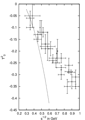
Now, we consider amplitude . This evaluated using (36) and plotted in Fig.3 along with the results obtained using the experimental phase shifts from [24]. It is seen from the Fig.3, that our theoretical amplitude upto are in reasonable agreement with the experimental amplitude calculated from the phase shifts. In this case, the lowest inelastic process is and as the -meson mass is 770 MeV, the above description is inadequate after this value for as we have not taken into account the rho production.
We now consider amplitude . This is evaluated using (36) with and and is plotted in Fig.4, along with the experimental amplitude calculated using the phase shifts from [24]. The agreement with the experiment is reasonable. The amplitude can be calculated from (36). However, as seen in [24] (their Fig.7.1c), the phase shifts are near zero till about 1 GeV. The theoretical values are consistent with zero.
To summarize, we have considered the holographic large QCD proposed by Sakai and Sugimoto and restricting to the pion sector, evaluated the effective action upto terms. The effective chiral lagrangian for pions is derived and this coincides with the lagrangian suggested by Weinberg. The couplings of the four derivative contact terms are determined in terms of . In the spirit of large , these couplings are re-expressed in terms of the pion decay constant, Kaluza-Klein scale and . Using and , we find that gives the amplitude within the unitarity bound. For these values, the partial wave amplitudes are evaluated and compared with the results obtained from experimental phase shifts. The agreement with the experimental data is found to be satisfactory within about 20 percent. It will be interesting to consider baryons within this approach and examine the baryon-meson coupling. This work is under progress.
Acknowledgement
One of us (K.S.V) acknowledges the warm hospitality at the Chennai Mathematical Institute. This research is supported by an operating grant from Natural Sciences and Engineering Council of Canada. Useful correspondence with J.R.Peláez is acknowledged with thanks.
References
- 1.
S.Weinberg, Physica A96, 327 (1979).
- 2.
S.Weinberg, Phys.Rev.Lett. 17, 616 (1966).
- 3.
S.M.Roy, Phys.Lett. 36, 353 (1971).
- 4.
F.Sannino and J.Schechter, Phys.Rev. D52, 96 (1995).
- 5.
B.Ananthanarayanan and P.Buttiker, “Pion-Pion scattering in Chiral Perturbation and Dispersion Relation Theories”, arXiv:hep-ph/9902461.
- 6.
J.Gasser and H.Leutwyler, Ann.Phys. (N.Y). 158, 142 (1984); Nucl.Phys. B250, 465 (1985).
- 7.
G.Colangelo, J.Gasser and H.Leutwyler, Nucl.Phys. B603, 125 (2001).
- 8.
J.R.Peláez and F.J.Ynduráin, Phys.Rev. D71, 074016 (2005).
- 9.
J.M.Maldacena, Adv.Theor.Math.Phys. 2, 331 (1998); arXiv:hep-th/9711200.
- 10.
S.S.Gubser, I.R.Klebanov and A.M.Polyakov, Phys.Lett. B428, 105 (1998); arXiv:hep-th/9802109. E.Wittn, Adv.Theor.Math.Phys. 2, 253 (1998); arXiv:hep-th/9802150. O.Aharony, S.S.Gubser, J.M.Maldacena, H.Ooguri and Y.Oz, Phys.Rep. 323, 183 (200); arXiv:hep-th/9905111.
- 11.
T.Sakai and S.Sugimoto, Prog.Theor.Phys. 113, 843 (2005); arXiv:hep-th/ 0412141.
- 12.
T.Sakai and S.Sugimoto, Prog.Theor.Phys. 114, 1083 (2006); arXiv:hep-th/ 0507073.
- 13.
D.K.Hong, M.Rho, H-U.Yee and P.Yi, “Chiral Dynamics of Baryons from String Theory”, arXiv:hep-th/0701276.
- 14.
D.K.Hong, M.Rho, H-U.Yee and P.Yi, “Dynamics of Baryons from String Theory and Vector Dominance”, arXiv: hep-th/07052632.
- 15.
H.Hata, T.Sakai, S.Sugimoto and S.Yamato, “Baryons from Instantons in holographic QCD”, arXiv: hep-th/0701280.
- 16.
K.Nawa, H.Suganuma and T.Kojo, “Baryons in holographic QCD”, arXiv: hep-th/ 0612187.
K.Hashimoto, T.Hirayama and A.Miwa, “Holographic QCD and Pion Mass”, arXiv: hep-th/0703024. - 17.
M.Kruczenski, D.Mateos, R.C.Myers and D.J.Winters, JHEP, 5, 041 (2004); arXiv: hep-th/0311270.
- 18.
O.Aharony, J.Sonnenschein and S.Yankielowicz, “A Holographic Model of Deconfinement and Chiral Symmetry Restoration” , arXiv: hep-th/0604161.
- 19.
T.H.R.Skyrme, Proc.Roy.Soc.Lond. A260, 127 (1961); Nucl.Phys. 31, 556 (1962).
- 20.
M.Harada, F.Sannino and J.Schechter, Phys.Rev. D54, 1991 (1996); D69, 034005 (2004), M.Harada, PiPi scattering and scalar mesons in an effective chiral lagrangian, hep-ph/0009051.
- 21.
M.Harada, S.Matsuzaki and K.Yamawaki, Phys.Rev. D74, 076004 (2006).
- 22.
M.Bando,T.Kugo, S.Uehara, K.Yamawaki and T.Yanagida, Phys.Rev.Lett. 54, 1215 (1985); M.Harada, T.Kugo and K.Yamawaki, Prog.Thoer.Phys. 91, 801 (1994).
- 23.
A.A.Tseytlin, Nucl.Phys. B501, 41 (1997).
- 24.
S.Nagaoka, Prog.Theo.Phys. 110, 1219 (2004).
- 25.
R.Parthasarathy and K.S.Viswanathan, “ Corrections in Holographic Large QCD and Scattering”, arXiv: hep-th/0707512.
- 26.
O.Bergman, S.Seki and J.Sonnenschein, “Quark mass and condensates in HQCD”, arXiv: hep-th/0708.2839; A.Dhar and P.Nag, “Sakai-Sugimoto model, tachyon condensation and chiral symmetry breaking”, arXiv: hep-th/0708.3233.
- 27.
R.Kamiński, J.R.Peláez and F.J.Ynduráin, “The pion-pion scattering amplitude. III: Improving the analysis with forward dispersion relations and Roy equations”, arXiv: hep-ph/0710.1150.
- 28.
D.Black, A.H.Fariborz, S.Moussa, S.Nasri and J.Schechter, Phys.Rev. D64, 014031 (2001). D.Black and J.Gaunt, “Study of scalar mesons in chiral Lagrangian frameworks”, arXiv: hep-ph/0801.2472.