Theory of resonant multiphonon Raman scattering in graphene

Since graphene is a non-polar crystal, Raman scattering involves electronic excitations as intermediate states: the electromagnetic field of the incident laser beam interacts primarily with the electronic subsystem, and emission of phonons occurs due to electron-phonon interaction. The matrix element of the process can be schematically represented as

Here $|i\rangle$ is the initial state of the process (the incident photon with a given frequency and polarization, and no excitations in the crystal), $|f\rangle$ is the final state (the emitted photon and $n$ phonons left in the crystal), while $s_{k}$, $k=0,\ldots,n$, label the intermediate states where no photons are present, but an electron-hole pair is created in the crystal and $k$ phonons have been emitted. $E_{i}$ and $E_{k}$, $k=0,\ldots,n$ are the energies of these states, and $2\gamma$ is the inverse lifetime of the electron (hole) due to collisions. $\hat{H}_{e-em}$ and $\hat{H}_{e-ph}$ stand for the terms in the system hamiltonian describing interaction of electrons with the electromagnetic field and with phonons, respectively.

In the calculations we do not include the phonon broadening, assuming the phonon states to have zero width. First, this approximation is consistent with the available experimental information: the phonon width is about $10-20\>\mathrm{cm}^{-1}\approx{2}-3\>\mathrm{meV}$ at most,[9, 10] while the electronic broadening is at least an order of magnitude higher (see the discussion below, Sec. II.3). Second, this approximation is irrelevant provided that we calculate the integrated intensities of the Raman peaks, since they are determined by the total spectral weight of the phonon state which does not depend on the phonon broadening.

The photon wave vector is negligible, so momentum conservation requires that the sum of the wave vectors of emitted phonons must vanish (provided that the impurity scattering is neglected). For the same reason Raman scattering on one intervalley phonon must be impurity-assisted [process (b) in Fig. 1, giving rise to the so-called $D$ Raman peak]. $D$ peak is absent in the experimental Raman spectrum of graphene,[6] showing that impurity scattering is indeed negligible in these samples.

Looking at the intermediate electronic states involved in the Raman scattering (Fig. 1), we notice that for one-phonon scattering [processes (a), (b)] at least one intermediate state must be virtual, since energy and momentum conservation cannot be satisfied simultaneously in all processes. Thus, at least one of the factors in the denominator of Eq. (1) must be of the order of the phonon frequency $\omega_{ph}$ [for the impurity assisted scattering one of the electron-phonon matrix elements in the numerator of Eq. (1) should be replaced by the electron-impurity matrix element]. For the two-phonon scattering [process (c)] all intermediate states can be real, so that all energy mismatches in the denominator of Eq. (1) can be nullified simultaneously and the result is determined by the electron scattering rate $2\gamma$. We emphasize the qualitative difference between the fully resonant process (c) and the double-resonant[13] process (b), where one intermediate state is still virtual. We also note the analogous difference between the two-phonon processes (c) and (d) in Fig. 1: only the process (c) is fully resonant, the other one involves an energy mismatch of $2\omega_{ph}$. As a result, its amplitude will be smaller by a factor $\sim\gamma/\omega_{ph}$.

Obviously, these arguments can be extended to all multi-phonon processes with odd and even number of phonons involved: in order to annihilate radiatively, the electron and the hole must have opposite momenta; if the total number of emitted phonons is odd, the electron and the hole must emit a different number of phonons, which is incompatible with energy conservation in all processes. Our main focus will thus be on even-phonon processes, as their intensities are determined by the electronic scattering.

The full resonance picture presented above assumes the mirror symmetry between the electron and the hole spectra. The electron-hole asymmetry can be included as a correction to the Dirac spectrum: the electron and the hole energies can be written as $vp\pm\alpha_{0}{p}^{2}$, where $p$ is the momentum counted from the Dirac point, $v$ is the Dirac velocity, and $\alpha_{0}$ is the asymmetry parameter. The energy scale $\Delta_{eh}$, quantifying the role of the asymmetry in the Raman scattering is defined as $\Delta_{eh}=\alpha_{0}(\omega_{in}^{2}-\omega_{out}^{2})/(2v)^{2}$, where $\omega_{in}$ and $\omega_{out}$ are the frequencies of the incident and the scattered photon (the details are given in Secs. VI.2, VII.3). Namely, the arguments of the previous paragraph hold if $\Delta_{eh}\ll\gamma$. In the opposite case, it is $\Delta_{eh}$ that determines the smallest value of the denominators in Eq. (1). We will always assume that both $\gamma,\Delta_{eh}\ll\omega_{ph}$.

In the real space, the typical size of the region of space probed by the electron-hole pair in the fully resonant two-phonon Raman scattering, is $\sim{v}/\max\{\gamma,\Delta_{eh}\}$. For the doubly resonant defect-induced one-phonon scattering, the inverse energy mismatch $1/\omega_{ph}$ determines the time duration of the process by virtue of the uncertainty principle, so the length scale of the process in the real space is $v/\omega_{ph}$. Although this length scale is much shorter than $v/\gamma$, it is still much greater than the lattice constant or the electron wavelength $v/\epsilon$.

The fully resonant Raman scattering, where the energy is conserved in each of the elementary scattering processes, admits a simple quasiclassical description, described qualitatively in this subsection, and justified rigorously in Secs. VI,VII.

Let us denote by $\epsilon$ the energy of the electron and the hole in the photoexcited pair. Initially, it is given by the half of the excitation frequency $\omega_{in}$, $\epsilon=\omega_{in}/2\sim{1}\;\mathrm{eV}$. After the emission of $n$ phonons it is decreased by $n\omega_{ph}$; assuming $\omega_{ph}\leq{0}.2\>\mathrm{eV}\ll\epsilon$, we neglect this decrease in the qualitative considerations. Thus, during all the time taken by the Raman scattering, electron and hole can be viewed as wave packets of the size $\sim{v}/\epsilon$, propagating across the crystal along classical trajectories.

The electron and the hole are created in the same region of space of the size $\sim{v}/\epsilon$ around some point ${\rm\bf r}_{0}$ at the moment of the arrival of the excitation photon. At this initial moment they have opposite momenta ${\rm\bf p},-{\rm\bf p}$, and opposite velocities ${\rm\bf v},-{\rm\bf v}$ (if the electron-hole asymmetry is taken into account, the two velocities will have slightly different magnitude), so they move along the straight lines, their positions being ${\rm\bf r}_{e}(t)={\rm\bf r}_{0}+{\rm\bf v}t$, ${\rm\bf r}_{h}(t)={\rm\bf r}_{0}-{\rm\bf v}t$. After a typical time $t\sim{1}/\gamma$ they undergo some scattering processes (e. g., phonon emission), where their momenta and (generally speaking) energies are changed. Each such elementary scattering process occurs during a short time $\sim{1}/\epsilon\ll{1}/\gamma$. Thus, the trajectories of the electron and the hole after their creation are represented by broken lines, with the typical segment length $\sim{v}/\gamma$ (the electron mean free path). The crucial point is that in order to recombine radiatively and contribute to Raman signal, the electron and the hole should meet again within a spatial region of the size $\sim{v}/\epsilon$, and have opposite momenta. The latter condition automatically implies that the number of the phonons emitted by the electron and the hole is the same. These considerations are illustrated by Fig. 2.

In the presence of a significant electron-hole asymmetry, $\Delta_{eh}\gg\gamma$, the described picture is modified. Namely, one of the segments of either the electron or the hole trajectory has the length $v/\Delta_{eh}$ instead of $v/\gamma$, the corresponding time travelling being restricted by the phase mismatch rather than by collisions.

For the single-phonon Raman peaks the commonly accepted notations are “$G$” for the peak at $1580\>\mathrm{cm}^{-1}$ corresponding to emission of an optical phonon with zero wave vector, and “$D$” for the defect-induced peak at $1350\>\mathrm{cm}^{-1}$ corresponding to emission of an optical phonon with the wave vector near $K$ or $K^{\prime}$ points of the Brillouin zone.[2] Sometimes one also distinguishes the so-called $D^{\prime}$-peak at $1620\>\mathrm{cm}^{-1}$. This peak is also defect-induced, and corresponds to emission of an optical phonon with a small wave vector $q\sim\epsilon/v$. As mentioned above, in the present work we study only the clean graphene, hence $D$ and $D^{\prime}$ peaks are of no interest to us.

Unfortunately, there is no single commonly accepted system for labelling of the multiphonon Raman peaks. The strong peak at $2700\>\mathrm{cm}^{-1}$, corresponding to emission of two phonons with the opposite wave vectors near the $K$ and $K^{\prime}$ points, was historically called $G^{\prime}$ (as it is not defect-induced); sometimes it is denoted by $2D$ or by $D^{*}$ to stress that it is the second overtone of the $D$ peak. The peak at $3250\>\mathrm{cm}^{-1}$ corresponding to emission of two phonons with two opposite wave vectors near the $\Gamma$ point is sometimes called $G^{*}$, $2G$ or $2D^{\prime}$. The latter notation reflects the fact that the frequency of this peak is not exactly the double of that of the $G$ peak, but rather the double of the defect-induced $D^{\prime}$ peak.

In the following we use the notation $n\Gamma+mK$ to denote the peak corresponding to emission of $n$ phonons with wave vectors within $\sim\epsilon/v$ from the $\Gamma$ point and of $m$ phonons with wave vectors within $\sim\epsilon/v$ from the $K$ or $K^{\prime}$ points. For multiphonon peaks this nomenclature is unambiguous. Thus, the peaks at $2700\>\mathrm{cm}^{-1}$ and at $3250\>\mathrm{cm}^{-1}$ will be called $2K$ and $2\Gamma$, respectively.

In the clean graphene the only one-phonon Raman process, allowed by the momentum conservation corresponds to the emission of the $E_{2}$ optical phonon with zero wave vector and frequency $1580\>\mathrm{cm}^{-1}$. For this process the situation turns out to be drastically different from that described by the qualitative considerations of Sec. I.1. As shown in Sec. V, if one approximates the electron spectrum by the Dirac cones, the numerator of Eq. (1) vanishes due to high symmetry of the low-energy electronic Dirac hamiltonian (as compared to the microscopic symmetry of the crystal). Thus, the main contribution to the Raman amplitude comes from the regions of the electronic Brillouin zone far from the Dirac points. As a consequence, the typical energy mismatch in the denominator of Eq. (1) is of the order of the whole electronic bandwidth. Thus, the Raman process, responsible for the $1580\>\mathrm{cm}^{-1}$ peak, is completely off-resonant and the picture shown in Fig. 1 for the process (a) is wrong.

As a result, the intensity of the peak is expected to be insensitive to most external parameters: polarization, electron concentration, degree of disorder, etc. To characterize this intensity, one has to introduce an additional parameter into the theory which has no simple relation to the parameters of the low-energy effective hailtonian. The resulting intensity of the peak is given by Eq. (60); it is proportional to the fourth power of the excitation frequency which is the standard result for Raman scattering when the difference between the frequencies of the incident and scattered photons is small. This dependence also agrees with the experimental results of Ref. 14.

Note that the results described above do not hold for the defect-induced peak at $1350\>\mathrm{cm}^{-1}$. For this peak the double resonance picture,[13] shown in Fig. 1, process (b), is fully adequate.

As the phonons are emitted by electrons with momentum $\omega_{in}/(2v)$, the largest possible phonon momentum is $q_{max}=(\omega_{in}+\omega_{out})/2v$, corresponding to the electron and hole backscattering (for the $2K$ peak at 2700 cm^-1 we count the phonon momenta from the $K$ and $K^{\prime}$ points). It would be natural to expect that any pair of phonons with opposite momenta ${\rm\bf q},-{\rm\bf q}$ and $|{\rm\bf q}|\leq{q}_{max}$ can be emitted, the only exception being ${\rm\bf q}=0$ which is prohibited by symmetry[2] and the nearby ones which are suppressed due to the smallness of the matrix elements. These arguments would predict the width of the peak to be of the order of $(v_{ph}/v)\omega_{in}$, where $v_{ph}$ is the $K$ phonon group velocity; besides, the shape of the peak would be strongly asymmetric: a sharp cutoff on the high-energy side at the frequency $2\omega_{ph}(q_{max})$ due to the resonance restriction, and a smooth drop-off towards zero at $2\omega_{ph}(q=0)$ due to the matrix element suppression. The phonon dispersion can be deduced from the dependence of the frequency of the impurity-assisted one-phonon $D$ peak in graphite on the excitation energy $\omega_{in}$: $d\omega_{ph}/d\omega_{in}=v_{ph}/v\approx{50}\>\mathrm{cm}^{-1}/\mathrm{eV}$.[15, 16, 17, 18] Thus, for $\omega_{in}=2$ eV these arguments give the width of the $2K$ peak to be about $200$ cm^-1. However, the experimentally observed width is only about 30 cm^-1 at $\omega_{in}=2.2$ eV, and its shape is quite symmetric.[6, 9]

The observed small width of the peak is explained by the quasiclassical picture, presented in Sec. I.2. If upon the emission of phonons the electron and the hole are scattered by an arbitrary angle, as shown in Fig. 2(b), they will not be able to meet at the same spatial point in order to recombine radiatively and contribute to the two-phonon Raman peak. Only if the scattering is backwards, this event is possible, as illustrated by Fig. 2(c). This condition fixes the wave vectors of the emitted phonons to be $q=q_{max}=2\epsilon/v$. The small deviations of the scattering angle from $\pi$ are restricted by the quantum diffraction, and the width of the two-phonon Raman peaks, instead of being $\sim(v_{ph}/v)\omega_{in}$, is determined by a much smaller energy scale (see the discussion below).

The dominance of the electron and hole backscattering manifests itself in the polariazion memory of the Raman signal. If the incident light is linearly polarized, the probability of excitation of the electron-hole pair with a given direction of momenta is proportional to $\sin^{2}\varphi$, where $\varphi$ is the angle between the electric field vector of the light and the momenta. Thus, upon backscattering and radiative recombination, the probability to detect a photon of the same polarization as the original one is $\propto\sin^{4}\varphi$, and that of the orthogonal polarization is $\propto\sin^{2}\varphi\cos^{2}\varphi$. Averaging over $\varphi$, we obtain the ratio of intensities for the detection of polarization parallel and perpendicular to that of the incident light to be $I_{\|}/I_{\perp}=3$. This ratio may be slightly decreased due to a finite aperture (see the discussion in Sec. IV.2).

The calculation of the intensities of the two-phonon Raman peaks is performed in Sec. VI. The explicit expressions for the intensities of the $2K$ and $2\Gamma$ peaks, obtained under the assumption of Dirac spectrum for the electrons, are represented by Eqs. (71) and (74). Both are proportional to $1/\gamma^{2}$, where $2\gamma$ is the electron (hole) inelastic scattering rate. If the latter is smaller that the electron-hole asymmetry $\Delta_{eh}$, then, according to the arguments of Sec. I.1, it is $\Delta_{eh}$ that restricts the energy denominators from below. Formally, this results in the replacement (80) in both Eqs. (71), (74).

Numerically, $\alpha_{0}(1\;\mbox{eV})^{2}/v^{2}\sim{0}.1\;\mbox{eV}$ (see, e. g., Ref. 19), so the relative correction to Eq. (71) for small $\Delta_{eh}$ can be estimated as $-(1/2)\Delta_{eh}^{2}/(2\gamma)]^{2}/2\sim-{10}^{-4}(\omega_{in}/2\gamma)^{2}$. The total electronic broadening $2\gamma$ was measured by time-resolved photoemission spectroscopy to be 20 meV in Ref. 20 and $25$ meV in Ref. 21 (all values taken for $\epsilon=\omega_{in}/2=1$ eV). A recent angle-resolved photoemission spectroscopy (ARPES) measurement gives a significantly larger value for $2\gamma\sim{100}\>\mbox{meV}$ (Ref. 22). Thus, the case $\gamma\gg\Delta_{eh}$ seems to be more relevant for the description of experiments, than the opposite one.

The Raman matrix element corresponding to emission of two phonons with given wave vectors ${\rm\bf q}$ and $-{\rm\bf q}$ is given by Eq. (69) for $\gamma\gg\Delta_{eh}$. From this dependence one can deduce the lineshape of the two-phonon peaks $2K,2\Gamma$:

where $\mu=K,\Gamma$, $2\omega_{\mu}$ is the central frequency for each peak, and $v_{ph,\mu}$ is the group velocity of the corresponding phonon. Thus, the full width at half maximum (FWHM) of each peak is given by

For $\gamma\ll\Delta_{eh}$ the dependence of the Raman matrix element on $q$ is described by Eq. (78). The lineshape corresponds to two peaks separated by $(v_{ph,\mu}/v)4\Delta_{eh}$. Experimentally, one sees just one $2K$ peak with the FWHM about 30 cm^-1 at the excitation frequency $\omega_{in}\approx{2}\>\mathrm{eV}$.[6, 9] This corresponds to an unrealistically large value of $2\gamma\sim{0.2}\>\mathrm{eV}$. Most likely, this indicates that two-phonon peaks are broadened by other mechanisms, not taken into account in the present work. In particular, Eq. (2) neglects (i) the broadening of the phonon states, and (ii) the anisotropy of the phonon dispersion (trigonal warping of the phonon spectrum). A detailed study of these effects would require introduction of additional parameters into the theory, so we prefer to postpone such study for the future work. It is worth emphasizing again that the integrated intensity of the peaks, which is the main focus of the present study, does not depend on these details.

In view of the results of the present paper it is worth mentioning the experimental measurements of the intensity $I_{2K}$ as a function of doping. While in Ref. 9 no significant dependence was observed, Ref. 12, where higher doping levels were reached, shows quite a strong dependence of $I_{2K}/I_{\Gamma}$ on doping. The intensity $I_{\Gamma}$ of the off-resonant single-phonon $1580\>\mathrm{cm}^{-1}$ peak should not depend on doping (although the phonon width does exhibit such a dependence, the total spectral weight of the phonon state, determining the integrated intensity of the peak, must be preserved). At the same time, the intensity $I_{2K}$, if determined by the electron inelastic lifetime, should be sensitive to the concentration of carriers. Indeed, in the intrinsic graphene at low temperatures the photoexcited carriers do not participate in electron-electron collisions, as the phase space volume is restricted.[23] As the carriers are added to the system, the electron-electron collisions become possible, thus the total $\gamma$ increases, and the intensity $I_{2K}$ is decreased, in qualitative agreement with the observation of Ref. 12.

The motivation to study the four-phonon Raman process comes from the following picture for the fully resonant processes. The incident photon creates an electron and a hole – real quasiparticles which can participate in various scattering processes. If the electron emits a phonon with a momentum ${\rm\bf q}$, the hole emits a phonon with the momentum $-{\rm\bf q}$, and after that the electron and the hole recombine radiatively, the resulting photon will contribute to the two-phonon Raman peak. If they do not recombine at this stage, but each of them emits one more phonon, and they recombine afterwards, the resulting photon will contribute to the four-phonon peak, etc. Three-phonon processes, not being fully resonant, are not interesting in this context.

Besides phonon emission and radiative recombination, electron and hole are subject to other inelastic scattering processes, which can also be viewed as emission of some excitations of the system. In principle, Raman spectrum should also contain the contrubution from these excitations, which are left in the system after the radiative recombination of the electron and the hole. The key point is that for real quasiparticles, the probability to undergo a scattering process $\alpha$ is determined by the ratio of corresponding scattering rate $2\gamma_{\alpha}$ to the total scattering rate $2\gamma\equiv\sum_{\alpha}{2}\gamma_{\alpha}$, not by the history. This probability determines the relative frequency-integrated intensity of the corresponding feature in the Raman spectrum. Thus, the ratio of integrated intensity $I_{(2n+2)K}$ of the Raman peak corresponding to $2n+2$ $K$ phonons to that for $2n$ $K$ phonons ($I_{2nK}$) must be proportional to $(\gamma_{K}/\gamma)^{2}$, where $2\gamma_{K}$ is the rate of emission of each of the two $K$ phonons, and the square comes from the phonon emission by the electron and the hole. This conclusion depends weakly on the relation between $\gamma$ and $\Delta_{eh}$, only through a logarithmic factor.

In the doped graphene, the most obvious competitor of the phonon emission is the electron-electron scattering: the optically excited electron can kick out another one from the Fermi sea, i. e., to emit another electron-hole pair. Thus, Raman spectrum should contain contribution from electron-hole pairs; however, their spectrum extends all the way to the energy of the photo-excited electron (optical energy) in a completely featureless way. Thus, it cannot be distinguished from the parasitic background which is always subtracted in the analysis of Raman spectra, and cannot be seen in the Raman spectrum directly. However, assuming $\gamma=\gamma_{K}+\gamma_{\Gamma}+\gamma_{ee}$, where $2\gamma_{\Gamma}$ is the rate of emission of phonons from the vicinity of the $\Gamma$ point of the first Brillouin zone, and $2\gamma_{ee}$ is the electron-electron collision rate, one can extract the value of $\gamma_{ee}$, relative to phonon emission rates from the experimental data. More precisely, in this way one obtains the rate of all inelastic scattering processes where the electron loses energy far exceeding the phonon energy.

Note that arguments leading to $I_{(2n+2)K}/I_{2nK}\propto(\gamma_{ph}/\gamma)^{2}$ are not specific for graphene; in fact, this is nothing but Breit-Wigner formula, applied once for the electron and once for the hole. Multi-phonon Raman scattering has been studied in wide-gap semiconductors both experimentally [24, 25] (up to ten phonons were seen in the Raman spectra of CdS), and theoretically [26, 27]. In a wide-gap semiconductor an optically excited electron does not have a sufficient energy to excite another electron across the gap, so the electron-electron channel is absent. In addition, interaction with only one phonon mode is dominant, so the ratios of subsequent peaks are represented by a sequence of fixed numbers. The simple band structure (one valley for CdS in contrast to two valleys for graphene) allowed a calculation of the whole sequence. A more complicated electronic band structure in graphene makes it problematic to calculate the whole sequence, so we restrict ourselves to the calculation of $I_{4K}$ for the most intense four-phonon peak.

This calculation is performed in Sec. VII. Its result depends, besides the relation between $\gamma$ and $\Delta_{eh}$, also on their relation to the energy scale $\omega_{in}(v_{ph}/v)$, characterizing the phonon dispersion. In Sec. II.3 we have already discussed this energy scale; for $\omega_{in}=2\>\mathrm{eV}$ we have $\omega_{in}(v_{ph}/v)\approx{1}00\>\mathrm{cm}^{-1}\approx{12}\>\mathrm{meV}$. The meaning of this energy scale is the difference between the energies of the electron and the hole after each of them has emitted two phonons with almost arbitrary momenta (the only restriction is that the sum of all four phonon momenta must vanish). If $\omega_{in}(v_{ph}/v)\ll\gamma,\Delta_{eh}$, which seems to be the case (see the discussion in the previous subsection) then this difference can be neglected, and the intensity of the $4K$ peak is given by Eq. (114) for $\gamma\gg\Delta_{eh}$ [which is likely to be the case relevant for most experiments, and which was reported in the short paper by the author (Ref. 28)], and by Eq. (117) for $\gamma\ll\Delta_{eh}$; the polarization memory is lost in both these cases, $I_{\|}\approx{I}_{\perp}$. In the case $\omega_{in}(v_{ph}/v)\gg\gamma,\Delta_{eh}$ the intensity $I_{4K}$ is given by Eq. (131), and a significant polarization memory is expected, up to $I_{\|}/I_{\perp}\approx{3}$.

A thorough experimental study of the intensity $I_{4K}$ (in particular, its dependence on doping) is still lacking. Our prediction for the case $\gamma\gg\Delta_{eh},\omega_{in}(v_{ph}/v)$, which we believe to be the experimentally relevant one, is[28, 57]

In the calculations of the Raman intensities, described above, electron-phonon coupling constants entered as parameters of the theory, without any assumptions about their values, except for the relations fixed by the symmetry of the crystal. In particular, the two-phonon peak intensities $I_{2K}$ and $I_{2\Gamma}$ are determined by two independent dimensionless coupling constants which we denote $\lambda_{K}$ and $\lambda_{\Gamma}$ [see Eq. (24) for the definition]. A simple estimate of the coupling constants can be obtained from the tight-binding nearest-neighbor model of the graphene crystal. In this model the only parameter characterizing the electron spectrum is the nearest-neighbor electronic matrix element $t_{0}$, and the electron-phonon interaction is characterized by its change with the bond length, $\partial{t}_{0}/\partial{a}$. In this model we obtain $\lambda_{K}/\lambda_{\Gamma}$ to be given by the inverse ratio of the corresponding phonon frequencies, about 1.2; the same result up to a few percent is obtained from the density-functional theory (DFT) calculations of Ref. 29. At the same time, by comparing the experimentally measured intensities of the different two-phonon peaks, and using the result of our calculation performed in Sec. VI, we can independently extract the ratio of the coupling constants. According to the data of Ref. 6, $I_{2K}/I_{2\Gamma}\approx{20}$, which gives $\lambda_{K}/\lambda_{\Gamma}\approx{3}$.

To explain this discrepancy we first analyzed the effect of the electronic trigonal band warping, which affects $I_{2K}$ and $I_{2\Gamma}$ differently. The corresponding calculation is done in Sec. VI.2. For $\omega_{in}=2$ eV, we estimate the relative contribution of the warping term as ${5}\cdot{10}^{-4}$ for $I_{2K}$ and $5\cdot{10}^{-2}$ for $I_{2\Gamma}$, which is far too little to account for the observed ratio $I_{2K}/I_{2\Gamma}$. We are thus led to the conclusion that the observed ratio $I_{2K}/I_{2\Gamma}$ must be due to the difference of the coupling constants, not accounted for by the DFT calculation. A similar conclusion about the insufficiency of the DFT calculation of the electron-phonon coupling constants has been drawn in Ref. 31, where an attempt was made to explain the experimental data obtained by ARPES[22] using the results of the DFT calculation.

At the same time, we should note that the dimensionless coupling constant $\lambda_{\Gamma}$ for the phonons near the $\Gamma$ point, as calculated by DFT[29] ($\lambda_{\Gamma}\approx{0}.028$), agrees reasonably well with the measured one: the measurements of the linear in the wave vector $q$ term in the phonon dispersion (Kohn anomaly due to electron-phonon interaction), $\omega_{ph}(q)-\omega_{ph}(q=0)\approx(\lambda_{\Gamma}/8)vq$, give $\lambda_{\Gamma}\approx{0}.024$ (see Ref. 30); the measurements of the dependence of the phonon frequency $\omega_{ph}$ on the electron Fermi energy $\epsilon_{F}$: $\Delta\omega_{ph}\approx(\lambda_{\Gamma}/2\pi)|\epsilon_{F}|$ give $\lambda_{\Gamma}\approx{0}.034$ (Ref. 9) $\lambda_{\Gamma}\approx{0}.027$ (Ref. 10).

We show that the difference between the ratio $\lambda_{K}/\lambda_{\Gamma}\approx{3}$ extracted from the Raman peak intensities, and $\lambda_{K}/\lambda_{\Gamma}\approx{1}.2$ obtained by the DFT calculation,[29] is due to the part of Coulomb interaction between electrons, not picked up by the DFT when local approximations are used for the exchange-correlation functional, such as the local density approximation (LDA) or the generalized gradient approximation (GGA), namely, logarithmic renormalizations.[39] Coulomb interaction has been known to be a source of logarithmic renormalizations for Dirac fermions.[32, 33, 34] Coulomb renormalizations in graphene subject to a magnetic field have been considered in Ref. 35, Coulomb effect on static disorder has been studied in Refs. 36, 37, 38. Essentially, the idea of the renormalization of the coupling constants is that the matrix element of the electron-phonon interaction should be taken not between the non-interacting electronic states, but between the states dressed by the Coulomb interaction. If the typical electronic energy in the problem is $\epsilon$ ($\sim{1}\>\mathrm{eV}$ in the case of Raman scattering), the renormalization is determined by the Coulomb interaction at all length scales from the shortest ones (lattice constant) to the electron wavelength $v/\epsilon$. It is this long-range part of the exchange and correlation that is missed by the local approximations in the DFT calculation, which take into account correctly only the short-range correlations (at the distances of the order of the lattice constant).

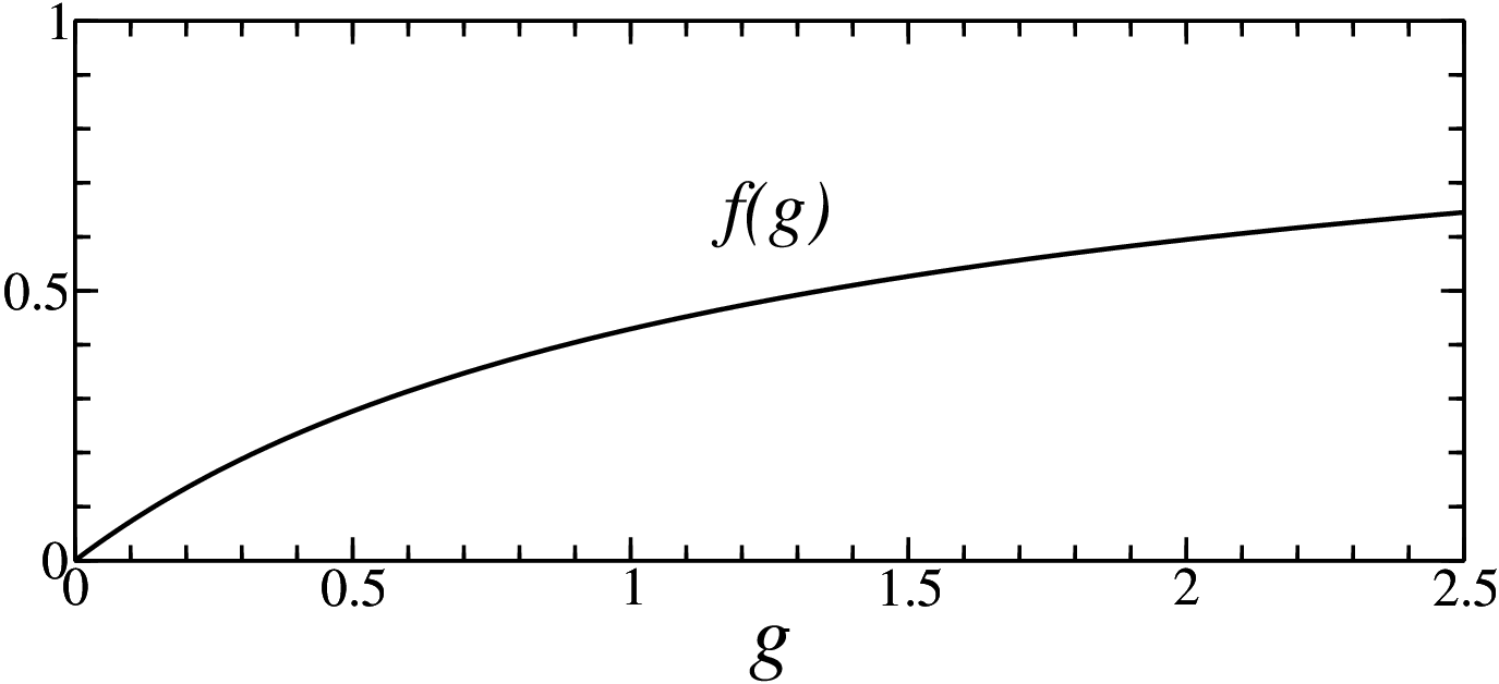
In Sec. VIII.1 we calculate the renormalization of the dimensionless electron-phonon coupling constants (a preliminary account of this work was given in the short paper[39]), and show that the coupling constant $\lambda_{\Gamma}$ for the phonons near the $\Gamma$ point is not renormalized (hence the agreement between the value of $\lambda_{\Gamma}$ calculated by the DFT and measured in the experiments, as mentioned above), while the coupling constant $\lambda_{K}$ for the phonons near the $K$ point, which is responsible for the $2K$ Raman peak, is enhanced by the Coulomb interaction. This enhancement depends on the electronic energy, as shown in Fig. 22. For the electronic energy $1\>\mathrm{eV}$ this enhancement is in quantitative agreement with the measured ratio $I_{2K}/I_{2\Gamma}$, provided that the screening of the Coulomb interaction by the substrate is weak. The dependence of the enhancement on the electronic energy translates into the dependence of $I_{2K}/I_{2\Gamma}$ on the excitation frequency, which can be checked experimentally. Similarly, as the Coulomb interaction is screened by the substrate with a dielectric constant $\varepsilon_{\infty}$ (its high-frequency value), the dependence of $I_{2K}/I_{2\Gamma}$ on $\varepsilon_{\infty}$ can also serve as an experimental check of the theory.

We also show in Sec. VIII.2 that the electron-phonon coupling itself is a source of logarithmic renormalizations. However, due to the smallness of the coupling constants this effect is much weaker than the effect of the Coulomb interaction.

In Sec. III the low-energy hamiltonian of the interaction of electrons with the crystal vibrations and the electromagnetic field is written from pure symmetry considerations. In Sec. III.1 the symmetry of the graphene crystal is reviewed. In Sec. III.2 the symmetry considerations are used to write the electronic part of the hamiltonian. Sec. III.3 is dedicated to the symmetry analysis of the Dirac part of the electron hamiltonian, whose symmetry is significantly higher than the symmetry of the crystal. Sec. III.4 is dedicated to the symmetry analysis of the in-plane crystal vibrations. In Secs. III.5 and III.6 we write the hamiltonian of interaction of electrons with the optical and acoustical vibrations, respectively. Sec. III.7 is dedicated to the symmetry analysis of the out-of-plane vibrations of the graphene crystal. In Sec. III.8 the hamiltonian of the interaction of electrons with the electromagnetic field is written.

Sec. IV describes the general scheme of the calculation of Raman peak intensities using the standard perturbation theory. In Sec. IV.1 the Green’s functions are introduced, and in Sec. IV.2 the general expression for the Raman scattering probability is derived. In Sec. IV.3 we discuss the electron inelastic scattering, and calculate the electronic self-energy due to the electron-phonon coupling.

In Sec. V one-phonon Raman scattering is discussed, and it is shown that the calculation of the one-phonon peak intensity cannot be performed within the low-energy theory. In Sec. VI the two-phonon Raman peak intensities are calculated, first, under the assumption of the Dirac electron spectrum (Sec. VI.1), and then taking into account the trigonal band warping and electron-hole asymmetry (Sec. VI.2). In Sec. VII the intensity $I_{4K}$ of the most intense four-phonon peak is calculated. Secs. VIII.1, VIII.2 are dedicated to the renormalization of the electron-phonon coupling constants due to Coulomb interaction and due to the electron-phonon interaction, respectively.

Since the typical energy of the incident photon (about $2$ eV) is much smaller than the $\pi$-electron bandwidth ($\sim{20}$ eV), one can expect the low-energy excitations to play the dominant role. In this section we employ standard symmetry analysis[41] to fix the form of the low-energy hamiltonian. We prefer not to choose any specific basis and use algebraic properties.

The carbon atoms of graphene form a honeycomb lattice with two atoms per unit cell, labeled $A$ and $B$ (Fig. 3), the distance between nearest neighbors being $a=1.42$ Å. Three out of four electrons of the outer shell of each carbon atom form strong $\sigma$ bonds with its three nearest neighbors, and represent no interest to us. The remaining $\pi$ orbitals (one per each carbon atom) give rise to the half-filled $\pi$ band.

In this paper we will not consider the dimension, perpendicular to the crystal plane, so the point symmetry group of the graphene crystal is $C_{6v}$. It contains 12 elements: the identity, five rotations $C_{6}^{n}$, $n=1,\ldots,5$ ($C_{m}$ denoting the rotation by $2\pi/m$) and six reflections in planes perpendicular to the crystal plane. The three reflections leaving the $A$ and $B$ sublattices invariant are denoted by $\sigma_{a},\sigma_{b},\sigma_{c}$, while those swapping the $A$ and $B$ sublattices points will be denoted by $\sigma_{a}^{\prime},\sigma_{b}^{\prime},\sigma_{c}^{\prime}$. Table 1 lists the irreducible representations of the group $C_{6v}$ and their characters.

The first Brillouin zone of the crystal is a hexagon (Fig. 4). Out of the six corners of the hexagon only two are inequivalent. They are called $K$ and $K^{\prime}$ points. The group of the wave vector at these points is $C_{3v}$. The states at these points are twice degenerate, transforming according to the two-dimensional irreducible representation ($E$) of $C_{3v}$. Transformations, swapping $K$ and $K^{\prime}$, thus belonging to $C_{6v}$ but not to $C_{3v}$, (reflection $\sigma_{v}$ in the plane, perpendicular to that of $\sigma_{v}^{\prime}$, and rotations $C_{2},C_{6}$), fix the energies at $K,K^{\prime}$ to be equal. One can form real linear combinations of wave functions from $K$ and $K^{\prime}$ points which transform according to $E_{1}$ and $E_{2}$ representations of $C_{6v}$. The degeneracy at $K,K^{\prime}$ points, in combination with the absence of any other states in the Brillouin zone with the same energy, fixes the Fermi level of a half-filled band to be at this energy, which is thus natural to choose as $\epsilon=0$.

Instead of dealing with degenerate states at two different points of the Brillouin zone ($K,K^{\prime}$), one can triple the unit cell of the crystal. The new unit cell contains 6 atoms which form a hexagon (Fig. 3), while the new Brillouin zone is only 1/3 of the original one (Fig. 4). The advantage of this approach is that now both $K$ and $K^{\prime}$ are mapped onto the $\Gamma$ point, so one does not have to consider the two of them separately.

Tripling of the unit cell means that two translations $t_{{\rm\bf a}_{1}}$ and $t_{{\rm\bf a}_{2}}$ are factorized out from the translation group of the crystal, so they should be added to the point group, which becomes $C_{6v}^{\prime\prime}=C_{6v}+(t_{{\rm\bf a}_{1}}C_{6v})+(t_{{\rm\bf a}_{2}}C_{6v})$. Irreducible representations of this group and their characters are shown on Table 2. The states of the $\pi$-electrons at the new $\Gamma$ point form a 6-dimensional representation which is reduced as $A_{1}+{B}_{2}+{G^{\prime}}$, where $A_{1}$ and $B_{2}$ states are the non-degenerate ones corresponding to the old $\Gamma$ point, while the 4-dimensional irreducible representation $G^{\prime}$ contains the zero-energy states inherited from the old $K,K^{\prime}$ points.

In order to write down the low-energy electronic hamiltonian, we have to consider $4\times{4}$ hermitian matrices acting in the 4-dimensional space of the zero-energy electronic states. The basis in the 16-dimensional space of such matrices is provided by the generators of the $SU(4)$ group forming a 16-dimensional reducible representation of $C_{6v}$ or $C_{6v}^{\prime\prime}$. This representation is reduced as

within the group $C_{6v}$ (the two sectors corresponding to matrices either diagonal or off-diagonal in the $KK^{\prime}$ subspace), or as

within the group $C_{6v}^{\prime\prime}$. The correspondence between Eqs. (5) and (6) is given in Table 3.

The most convenient way to identify the matrices is by specifying the irreducible representation according to which they transform, rather by specifying their explicit form in some particular basis. So, the matrix which transforms according to the $A_{2}$ representation of $C_{6v}^{\prime\prime}$ will be denoted by $\Sigma_{z}$ and called the $z$-component of the isospin (the only arbitrariness in this definition is the overall sign). The two matrices which transform according to the vector $E_{1}$ representation of $C_{6v}^{\prime\prime}$ will be denoted by $\{\Sigma_{x},\Sigma_{y}\}\equiv{\rm\bf\Sigma}$ [defined up to an arbitrary rotation, see Eq. (15a) below], and so on. The full list of definitions and notations is given in Table 3.

Explicit expressions for the electronic matrices are not needed, as long as their algebraic rules are specified. The simplest way to specify these rules is to express all the 16 matrices in terms of two sets, $\{\Sigma_{x},\Sigma_{y},\Sigma_{z}\}$ and $\{\Lambda_{x},\Lambda_{y},\Lambda_{z}\}$, and their products, where the matrices from the same set satisfy the Pauli matrix algebra, while matrices from different sets just commute. In Appendix A we show how these rules can be established, and give the explicit expressions for the matrices for some specific choices of the basis. We also note that $e^{(2\pi{i}/3)\Sigma_{z}}$ is the matrix of the $C_{3}$ rotation, $\Lambda_{x}\Sigma_{z}$ – of the $C_{2}$ rotation, $\Lambda_{z}\Sigma_{x}$ – of the $\sigma_{a}^{\prime}$ reflection, $\Lambda_{y}\Sigma_{y}$ – of the $\sigma_{a}$ reflection, and $e^{\pm({2}\pi{i}/3)\Lambda_{z}}$ are the matrices of the two elementary translations.

Since there are two $\pi$-orbitals per unit cell, the eigenfunctions for each wave vector ${\rm\bf k}$ in the Brillouin zone are given by $e^{i{\rm\bf k}{\rm\bf r}}\mathcal{U}_{{\rm\bf k},\pm}({\rm\bf r},z)$, where the two Bloch functions $\mathcal{U}_{{\rm\bf k},\pm}({\rm\bf r},z)$, periodic in ${\rm\bf r}=(x,y)$, are even and odd with respect to the reflection $\sigma_{a}^{\prime}$, and are normalized as

where $L_{x}L_{y}$ is the crystal area. It is more convenient to choose their linear combinations, localized near each carbon atom: $\mathcal{U}_{{\rm\bf k},A}=(\mathcal{U}_{{\rm\bf k},+}+\mathcal{U}_{{\rm\bf k},-})/\sqrt{2}$ and $\mathcal{U}_{{\rm\bf k},B}=(\mathcal{U}_{{\rm\bf k},+}-\mathcal{U}_{{\rm\bf k},-})/\sqrt{2}$. In this basis an arbitrary wave function $\Psi({\rm\bf r},z)$ involving only low-energy states can be written in terms of a four-component smooth envelope function $\psi({\rm\bf r})$, or its Fourier transform $\psi({\rm\bf p})$, $pa\ll{1}$, as

The low-energy effective electronic hamiltonian $H_{\mathrm{el}}({\rm\bf p})$ is defined as a $4\times{4}$ matrix whose matrix element between any two smooth envelope functions $\psi({\rm\bf r})$ and $\tilde{\psi}({\rm\bf r})$ coincides with the matrix element of the microscopic hamiltonian $\mathcal{H}_{\mathrm{el}}(-i{\rm\bf\nabla},-i\partial_{z};{\rm\bf r},z)$ including the periodic crystal potential, between the corresponding full wave functions $\Psi({\rm\bf r},z)$ and $\tilde{\Psi}({\rm\bf r},z)$ (see Appendix B for details):

Strictly speaking, the spin index should also be attached to the enevlope function $\psi({\rm\bf r})$. However, it would make the formulas more cumbersome, and we prefer to omit it, as none of the calculations of the present paper will concern a non-trivial spin structure. The only role of the spin will be to provide an additional degeneracy, which will be accounted for, and mentioned separately every time it will enter the calculations.

We expand the effective hamiltonian in powers of ${\rm\bf p}$: $H_{\mathrm{el}}({\rm\bf p})=H_{1}({\rm\bf p})+H_{2}({\rm\bf p})+\ldots$, where $H_{n}({\rm\bf p})=O(p^{n})$. One can write down different terms from symmetry considerations, taking into account that momentum components $p_{x},p_{y}$ transform according to $E_{1}$ (vector) representation of $C_{6v}$. The leading term in the hamiltonian, $H_{1}({\rm\bf p})$, must have the Dirac form:[42]

The coefficient $v$ turns out to be equal to $v\approx{10}^{8}\>\mathrm{cm/s}\>\approx{7}\>\mathrm{eV\cdot\mbox{\AA}}$; it can be related to the nearest-neighbor coupling matrix element $t$ of the tight-binding model as $v=3ta/2$. The four eigenstates of the hamiltonian (10) for each ${\rm\bf p}$ can be classified by the value ($\pm{1}$) of projection of the isospin ${\rm\bf\Sigma}$ on ${\rm\bf p}$, corresponding to the energies $\pm{v}|{\rm\bf p}|$. In other words, the hamiltonian (10) is diagonalized by a unitary transformation:

$\varphi_{{\rm\bf p}}=\arctan(p_{y}/p_{x})$ being the polar angle of the vector ${\rm\bf p}$.

Various perturbations of the Dirac hamiltonian (10) should also be classified according to Table 3. Only those containing the matrix $\Sigma_{z}$ will open a gap in the electron spectrum. Perturbations, not containing $\Sigma_{i}$, correspond to an energy shift of the whole spectrum (which may be accompanied by valley mixing, if $\Lambda$ matrices are involved). Perturbations, proportional to ${\rm\bf\Sigma}$, correspond to a momentum shift of the Dirac points, which can be viewed as a gauge vector potential.

The next term in the hamiltonian can be written by taking into account that the symmetric tensor $p_{i}p_{j}$ can be decomposed into $p^{2}$, transforming according to $A_{1}$, and $2p_{x}p_{y},p_{x}^{2}-p_{y}^{2}$, transforming according to $E_{2}$:

The first term describes electron-hole asymmetry; it vanishes in the nearest-neighbor tight-binding model, and appears only if coupling to the second nearest neighbors is included. The second term, corresponding to $E_{2}$ representation, is responsible for the so-called trigonal band warping. In the nearest-neighbor tight-binding model its value is given by $-3ta^{2}/8$.

At this point it is convenient to introduce the time-reversal operation whose action on the microscopic spinless wave function is defined by $\Psi({\rm\bf r})\mapsto\Psi^{*}({\rm\bf r})$. For the four-component envelope function $\psi({\rm\bf r})$ this definition translates into

where $U_{\mathcal{T}}$ is a unitary $4\times{4}$ matrix, with an additional requirement $U_{\mathcal{T}}U_{\mathcal{T}}^{*}=\openone$, whose explicit form depends on the choice of the basis. The action of time reversal on the effective electronic hamiltonian is defined by

Behavior of electronic matrices under the time reversal is listed in Table 3.

Time reversal symmetry of the hamiltonian does not add any new symmetries to the spectrum, as compared to those imposed by the spatial symmetry $C_{6v}$ (namely, $C_{3v}$ symmetry of the spectrum around each of $K,K^{\prime}$ points, and the mirror symmetry between the spectra at $K$ and $K^{\prime}$ points), because the action of the time reversal on the wave vector is identical to that of the $C_{2}$ rotation, ${\rm\bf K}+{\rm\bf p}\mapsto{\rm\bf K}^{\prime}-{\rm\bf p}$. However, some perturbations may lift the $C_{2}$ symmetry, while still preserving the time reversal one (see Secs. III.5 and III.8)

The Dirac hamiltonian (10) has a higher symmetry than the microscopic symmetry $C_{6v}$. The additional symmetries are (i) the full intravalley rotational symmetry $C_{\infty{v}}$:

which leaves $H_{1}({\rm\bf p})$ invariant; (ii) the chiral property:

which ensures the symmetry of the spectrum with respect to $\epsilon\to-\epsilon$ (i. e., particle-hole symmetry).

The intravalley “time reversal” symmetry, mentioned in Ref. 43, can be represented as a combination of the time reversal (13), the intravalley rotation (15a) by $\pi$, and the $C_{2}$ rotation:

Applying this operation twice results in a minus sign, since the matrix $\Lambda_{x}$ is odd under time reversal.

If one wishes to include the second-order hamiltonian (12), the $A_{1}$ term preserves only the rotational symmetry $C_{\infty{v}}$, while the $E_{2}$ term preserves only the chiral property (16).

There is quite extensive literature dedicated to the phonon modes of graphene and graphite, and their symmetry analysis (see, e. g., Ref. 2 and references therein). To make the presentation self-contained, we briefly repeat the facts which are necessary for the subsequent considerations.

The only phonons that can efficiently couple to the low-energy electronic states are those near the $\Gamma$ point (coupling electronic states in the same valley), and near the $K,K^{\prime}$ points (coupling electronic states in different valleys; note that ${\rm\bf K}-{\rm\bf K}^{\prime}$ is equivalent to ${\rm\bf K}^{\prime}$). As a result, each unit cell has four in-plane degrees of freedom (two per each carbon atom). At $\Gamma$ point one has two acoustic and two optical modes. Coupling of the acoustical modes with a wave vector ${\rm\bf q}$ to the electron motion must vanish as $q\to{0}$, and thus be small in the parameter $qa$, but we consider them for the sake of completeness. For eight modes at $K,K^{\prime}$ points it is more convenient to consider their real linear combinations which transform according to $A_{1}+{B}_{1}+{A}_{2}+{B}_{2}+{E}_{1}+{E}_{2}$ representations of the group $C_{6v}$. All twelve modes are shown in Fig. 5. They are linearly polarized, in contrast to the basis with a definite wave vector, which would have a circular polarization.

After having mixed the $K$ and $K^{\prime}$ modes, it is natural to switch to the tripled unit cell representation. Analogously to Eq. (8) for electrons, an arbitrary lattice displacement pattern, involving phonon states with wave vectors close either to $\Gamma$, or $K$, or $K^{\prime}$ points, can be expressed in terms of a smooth envelope function $u({\rm\bf r})$ or its Fourier transform $u({\rm\bf q})$. Since we have to specify two cartesian components of displacements for each of the six atoms in the tripled unit cell, $\delta\underline{x}=(\delta{x}_{1},\delta{y}_{1},\ldots,\delta{x}_{6},\delta{y}_{6})^{T}$, the envelope of normal coordinates $u({\rm\bf q})$ is a twelve-component vector:

where ${\rm\bf R}$ spans a discrete set of points, labeling different unit cells, and $\underline{\mathcal{X}}_{{\rm\bf q},\mu}$ is the pattern of displacements for the $\mu$th normal mode, normalized as

For ${\rm\bf q}=0$ the twelve normal modes $\underline{\mathcal{X}}_{{\rm\bf q}=0,\mu}$ are shown in Fig. 5. Introducing $\Pi_{\mu}({\rm\bf r})$, the canonically conjugate momentum to $u_{\mu}({\rm\bf r})$, we write the bare phonon hamiltonian as

References

• [1] L. I. Mandelshtam and G. S. Landsberg, Z. Phys. 50, 169 (1928); C. V. Raman and K. S. Krishnan, Nature 121, 501 (1928); ibid. 121, 619 (1928).
• [2] S. Reich and C. Thomsen, Phil. Trans. R. Soc. Lond. A 362, 2271 (2004).
• [3] J. Kastner, T. Pichler, H. Kuzmany, S. Curran, W. Blau, D. N. Weldon, M. Dlamesiere, S. Draper, and H. Zandbergen, Chem. Phys. Lett. 221, 53 (1994).
• [4] A. M. Rao, E. Richter, S. Bandow, B. Chase, P. C. Eklund, K. W. Williams, M. Menon, K. R. Subbaswamy, A. Thess, R. E. Smalley, G. Dresselhaus, and M. S. Dresselhaus, Science 275, 187 (1997).
• [5] K. S. Novoselov, A. K. Geim, S. V. Morozov, D. Jiang, Y. Zhang, S. V. Dubonos, I. V. Grigorieva, and A. A. Firsov, Science 306, 666 (2004).
• [6] A. C. Ferrari, J. C. Meyer, V. Scardaci, C. Casiraghi, M. Lazzeri, F. Mauri, S. Piscanec, D. Jiang, K. S. Novoselov, S. Roth, and A. K. Geim, Phys. Rev. Lett. 97, 187401 (2006).
• [7] A. Gupta, G. Chen, P. Joshi, S. Tadigadapa, and P. C. Eklund, Nano Lett. 6, 2667 (2006).
• [8] D. Graf, F. Molitor, K. Ensslin, C. Stampfer, A. Jungen, C. Hierold, and L. Wirtz, Nano Lett. 7, 238 (2007).
• [9] J. Yan, Y. Zhang, P. Kim, and A. Pinczuk, Phys. Rev. Lett. 98 166802 (2007).
• [10] S. Pisana, M. Lazzeri, C. Casiraghi, K. S. Novoselov, A. K. Geim, A. C. Ferrari, and F. Mauri, Nature Mat. 6, 198 (2007).
• [11] C. Casiraghi, S. Pisana, K. S. Novoselov, A. K. Geim, and A. C. Ferrari, Appl. Phys. Lett. 91, 233108 (2007).
• [12] A. Das, S. Pisana, S. Piscanec, B. Chakraborty, S. K. Saha, U. V. Waghmare, R. Yiang, H. R. Krishnamurhthy, A. K. Geim, A. C. Ferrari and A. K. Sood, arXiv:0709.1174.
• [13] C. Thomsen and S. Reich, Phys. Rev. Lett. 85, 5214 (2000).
• [14] L. G. Cançado, A. Jorio, and M. A. Pimenta, Phys. Rev. B 76, 064304 (2007).
• [15] R. P. Vidano, D. B. Fischbach, L. J. Willis and T. M. Loehr, Solid State Commun. 39, 341 (1981).
• [16] Y. Wang, D. C. Alsmeyer, and R. L. McCreery, Chem. Mater. 2, 557 (1990).
• [17] I. Pócsik, M. Hundhausen, M. Koos, and L. Ley, J. Non-Cryst. Solids 227–230, 1083 (1998).
• [18] M. J. Matthews, M. A. Pimenta, G. Dresselhaus, M. S. Dresselhaus, and M. Endo, Phys. Rev. B 59, R6585 (1999).
• [19] R. Saito, G. Dresselhaus, and M. S. Dresselhaus, Physical Properties of Carbon Nanotubes (Imperial College Press, London, 1998).
• [20] S. Xu, J. Cao, C. C. Miller, D. A. Mantell, R. J. D. Miller, and Y. Gao, Phys. Rev. Lett. 76, 483 (1996).
• [21] G. Moos, C. Gahl, R. Fasel, M. Wolf, and T. Hertel, Phys. Rev. Lett. 87, 267402 (2001).
• [22] A. Bostwick, T. Ohta, T. Seyller, K. Horn, and E. Rotenberg, Nature Physics 3, 36 (2007).
• [23] J. González, F. Guinea, and M. A. H. Vozmediano, Phys. Rev. Lett. 77, 3589 (1996).
• [24] R. C. C. Leite, J. F. Scott, and T. C. Damen, Phys. Rev. Lett. 22, 780 (1969).
• [25] M. V. Klein and S. P. S. Porto, Phys. Rev. Lett. 22, 782 (1969).
• [26] R. M. Martin and C. M. Varma, Phys. Rev. Lett. 26, 1241 (1971).
• [27] R. Zeyher, Solid State Commun. 16, 49 (1975).
• [28] D. M. Basko, Phys. Rev. B 76, 081405(R) (2007).
• [29] S. Piscanec, M. Lazzeri, F. Mauri, A. C. Ferrari, and J. Robertson, Phys. Rev. Lett. 93, 185503 (2004).
• [30] J. Maultzsch, S. Reich, C. Thomsen, H. Requardt, and P. Ordejón, Phys. Rev. Lett. 92, 075501 (2004).
• [31] M. Calandra and F. Mauri, Phys. Rev. B 76, 205411 (2007).
• [32] A. A. Abrikosov and S. D. Beneslavskii, Zh. Eksp. Teor. Fiz 59, 1280 (1970) [Sov. Phys. JETP 32, 699 (1971)].
• [33] J. González, F. Guinea, and M. A. H. Vozmediano, Mod. Phys. Lett. B 7, 1593 (1994); Nucl. Phys. B 424, 595 (1994); J. Low Temp. Phys. 99, 287 (1994).
• [34] J. González, F. Guinea, and M. A. H. Vozmediano, Phys. Rev. B 59, R2474 (1999).
• [35] I. L. Aleiner, D. E. Kharzeev, and A. M. Tsvelik, Phys. Rev. B 76, 195415 (2007)
• [36] J. Ye, Phys. Rev. B 60, 8290 (1999).
• [37] T. Stauber, F. Guinea, and M. A. H. Vozmediano, Phys. Rev. B 71, 041406(R) (2005).
• [38] M. S. Foster and I. L. Aleiner, arXiv:0802.0283.
• [39] D. M. Basko and I. L. Aleiner, Phys. Rev. B 77, 041409(R) (2008).
• [40] Secs. III and V of the present paper were written in coauthorship with I. L. Aleiner.
• [41] M. Lax, Symmetry Principles in Solid State and Molecular Physics (Dover, New York, 2001 or Wiley, New York, 1974).
• [42] P. R. Wallace, Phys. Rev. 71, 622 (1947).
• [43] H. Suzuura and T. Ando, Phys. Rev. Lett. 89 266603 (2002).
• [44] L. D. Landau and E. M. Lifshits Theory of elasticity (Pergamon Press, 1970), §25.
• [45] I. A. Luk’yanchuk and A. M. Bratkovsky, arXiv:0707.0466.
• [46] M. Lazzeri, S. Piscanec, F. Mauri, A. C. Ferrari, and J. Robertson, Phys. Rev. B 73, 155426 (2006).
• [47] M. Lazzeri and F. Mauri, Phys. Rev. Lett. 97, 266407 (2006).
• [48] A. H. Castro Neto and F. Guinea, Phys. Rev. B 75, 045404 (2007).
• [49] A. Grüneis, R. Saito, T. Kimura, L. G. Cançado, M. A. Pimenta, A. Jorio, A. G. Souza Filho, G. Dresselhaus, and M. S. Dresselhaus, Phys Rev. B 65, 155405 (2002).
• [50] V. B. Berestetskii, E. M. Lifshits, and L. P. Pitaevskii, Quantum electrodynamics (Pergamon Press, 1982), §79.
• [51] J. Maultzsch, S. Reich, and C. Thomsen, Phys. Rev. B 70, 155403 (2004).
• [52] Σp​h\Sigma^{ph} in graphite was considered long ago [F. Guinea, J. Phys. C: Solid State Phys. 14, 3345 (1981)], but the logarithmic divergence was not noted in that work.
• [53] I. L. Aleiner and K. B. Efetov, Phys. Rev. Lett. 97, 236801 (2006).
• [54] E. McCann, K. Kechedzhi, V. I. Fal’ko, H. Suzuura, T. Ando, and B. L. Altshuler, Phys. Rev. Lett. 97, 146805 (2006).
• [55] E. I. Blount, Physical Review 126, 1636 (1962).
• [56] The idea of this calculation was suggested to the author by M. S. Foster.
• [57] There is an overall factor of 2​π2\pi missing in Eq. (6) of Ref. 28, which affects all I2​KI_{2K}, I2​ΓI_{2\Gamma}, and I4​KI_{4K}, but not their ratios. Besides, there is a factor of π/4\pi/4 missing in Eq. (9) of Ref. 28, which affects the central result [Eq. (1) of Ref. 28]. Fortunately, π/4≈0.79\pi/4\approx{0}.79 is not very much different from unity.