跳到论文正文
W Papers独立论文阅读器 arXiv:0804.3239 论文正文 计算阅读时间 · 0%
引用这篇论文根据当前论文元数据生成,正式投稿前建议核对。


License: arXiv.org perpetual non-exclusive license
arXiv:0804.3239v1 [hep-ph] 21 Apr 2008

The economical SU​(3)C⊗SU​(3)L⊗U​(1)X\mathrm{SU}(3)_{C}\otimes\mathrm{SU}(3)_{L}\otimes\mathrm{U}(1)_{X} model

Journal: Advances in High Energy Physics
P. V. Dong Address: Theory Group, KEK, 1-1 Oho, Tsukuba, 305-0801, Japan Thanks: Email: pvdong@iop.vast.ac.vn; on leave from Institute of Physics, VAST, Vietnam    H. N. Long Address: Institute of Physics, VAST, P.O. Box 429, Bo Ho, Hanoi 10000, Vietnam Thanks: Email: hnlong@iop.vast.ac.vn
Abstract

In this report the SU​(3)C⊗SU​(3)L⊗U​(1)X\mathrm{SU}(3)_{C}\otimes\mathrm{SU}(3)_{L}\otimes{\mathrm{U}}(1)_{X} gauge model with minimal scalar sector, two Higgs triplets, is presented in detail. One of the vacuum expectation values uu is a source of lepton-number violations and a reason for mixing among charged gauge bosons—the standard model W±W^{\pm} and the bilepton gauge bosons Y±Y^{\pm} as well as among the neutral non-Hermitian bilepton X0X^{0} and neutral gauge bosons—the ZZ and the new Z′Z^{\prime}. An exact diagonalization of the neutral gauge boson sector is derived and bilepton mass splitting is also given. Because of these mixings, the lepton-number violating interactions exist in both charged and neutral gauge boson sectors. Constraints on vacuum expectation values of the model are estimated and u≃𝒪⁡(1)​GeV,v≃vweak=246​GeVu\simeq\mathcal{O}(1)\ \textrm{GeV},v\simeq v_{\mathrm{weak}}=246\ \textrm{GeV}, and ω≃𝒪⁡(1)​TeV\omega\simeq\mathcal{O}(1)\ \textrm{TeV}. In this model there are three physical scalars, two neutral and one charged, and eight Goldstone bosons—the needed number for massive gauge bosons. The minimal scalar sector can provide all fermions including quarks and neutrinos consistent masses in which some of them require one-loop radiative corrections.

Keywords: 
Extensions of electroweak gauge and Higgs sectors, Quark and lepton masses and mixing
PACS
12.60.Cn , 12.60.Fr , 12.15.Ff , 14.60.Pq

KEK-TH-1245

1 Introduction

In spite of all the successes of the standard model it is unlikely to be the final theory. It leaves many striking features of the physics of our world unexplained. In the following we list some of them which leads to the model’s extensions. In particular the models with SU​(3)C⊗SU​(3)L⊗U​(1)X\mathrm{SU}(3)_{C}\otimes\mathrm{SU}(3)_{L}\otimes{\mathrm{U}}(1)_{X} (3-3-1) gauge group are presented.

1.1 Generation Problem and 3-3-1 Models

In the standard model the fundamental fermions come in generations. In writing down the theory one may start by first introducing just one generation, then one may repeat the same procedure by introducing copies of the first generation. Why do quarks and leptons come in repetitive structures (generations)? How many generations are there? How to understand the inter-relation between generations? These are the central issues of the weak interaction physics known as the generation problem or the flavor question. Nowhere in physics this question is replied [1]. One of the most important experimental results in the past few years has been the determination of the number of these generations within the framework of the standard model. In the minimal electroweak model the number of generations is given by the number of the neutrino species which are all massless, by definition. The number of generations is then computed from the invisible width of the Z0Z^{0},

Γinv≡ΓZ0−(Γh+∑lΓl),\Gamma_{\rm inv}\equiv\Gamma_{Z^{0}}-(\Gamma_{h}+\sum_{l}\Gamma_{l}),

where ΓZ0\Gamma_{Z^{0}} denotes the total width, the subscript hh refers to hadrons and Γl\Gamma_{l} (l=e,μ,τ)(l=e,\ \mu,\ \tau) is the width of the Z0Z^{0} decay into an l​l¯l\bar{l} pair. If Γν\Gamma_{\nu} is the theoretical width for just one massless neutrino, the number of generations is Ngen=Nν=Γinv/ΓνN_{\rm\mathrm{gen}}=N_{\nu}=\Gamma_{\rm inv}/\Gamma_{\nu} and recent results give a value very close to three Ngen=2.99±0.03N_{\rm\mathrm{gen}}=2.99\pm 0.03 [2, 3] but we do not understand why the number of standard model generations is three.

The answer to the generation problem may require a radical change in our approaches. It could be that the underlying objects are strings and all the low energy phenomena will be determined by physics at the Planck scale. Grand Unified Theories (GUTs) have had a major impact on both cosmology and astrophysics; for cosmology they led to the inflationary scenario, while for astrophysics supernova, neutrinos were first observed in proton-decay detectors. It remains for GUTs to have impact directly on particle physics itself [4]. GUTs cannot explain the presence of fermion generations. On the other side, supersymmetry (SUSY) for the time being is an answer in search of question to be replied. It does not explain the existence of any known particle or symmetry. Some traditional approaches to the problem such as GUTs, monopoles and higher dimensions introduce quite speculative pieces of new physics at high and experimentally inaccessible energies. Some years ago there were hopes that the number of generations could be computed from first principles such as geometry of compactified manifolds but these hopes did not materialize.

A very interesting alternative to explain the origin of generations comes from the cancelation of chiral anomalies of a gauge theory in all orders of perturbative expansion, which derives from the renormalizability condition. This constrains the fermion representation content. Three perturbative anomalies have been identified [5] for chiral gauge theories in four dimensional space-time: (i) The triangle chiral gauge anomaly [6] must be cancelled to avoid violations of gauge invariance and the renormalizability of the theory; (ii) The global non-perturbative SU(2) chiral gauge anomaly, [7] which must be absent in order for the fermion integral to be defined in a gauge invariant way; (iii) The mixed perturbative chiral gauge gravitational anomaly [8, 9] which must be cancelled in order to ensure general covariance. The general anomaly-free condition is

Ai​j​k≡Tr⁡[{Ti,Tj}​Tk]=∑representationsTr⁡[{TLi,TLj}​TLk−{TRi,TRj}​TRk]=0,A^{ijk}\equiv\mathrm{Tr}[\{T^{i},T^{j}\}T^{k}]=\sum_{\rm representations}{\rm Tr}[\{T^{i}_{L},T^{j}_{L}\}T^{k}_{L}-\{T^{i}_{R},T^{j}_{R}\}T^{k}_{R}]=0, (1)

where TiT^{i} is the representation of the gauge algebra on the set of all left-handed fermion and anti-fermion fields put in a single column ψ\psi, and “Tr” denotes a sum over these fermion and anti-fermion species; TL,RiT^{i}_{L,R} are the coupling matrices of fermions ψL,R\psi_{L,R} to the current Jμi=ψ¯L​γμ​TLi​ψL+ψ¯R​γμ​TRi​ψRJ^{i}_{\mu}=\bar{\psi}_{L}\gamma_{\mu}T^{i}_{L}\psi_{L}+\bar{\psi}_{R}\gamma_{\mu}T^{i}_{R}\psi_{R}, respectively. The ii index runs over the dimension of a simple SU(nn) group, i=1,2,…,n2−1i=1,2,...,n^{2}-1, with a rank n−1n-1, and i=0i=0 for the Abelian factor.

First let us consider the relationship between anomaly cancelation and flavor problem in the standard model. The individual generations have the following structure under the SU​(3)C⊗SU​(2)L⊗U​(1)Y\mathrm{SU}(3)_{C}\otimes\mathrm{SU}(2)_{L}\otimes\mathrm{U}(1)_{Y} (3-2-1) gauge group,

(νa​L,la​L)\displaystyle(\nu_{aL},l_{aL}) ∼\displaystyle\sim (1,2,−1),la​R∼(1,1,−2),\displaystyle(1,2,-1),\hskip 14.22636ptl_{aR}\sim(1,1,-2),
(ua​L,da​L)\displaystyle(u_{aL},d_{aL}) ∼\displaystyle\sim (3,2,1/3),ua​R∼(3,1,4/3),da​R∼(3,1,−2/3).\displaystyle(3,2,1/3),\hskip 14.22636ptu_{aR}\sim(3,1,4/3),\hskip 14.22636ptd_{aR}\sim(3,1,-2/3). (2)

The values in the parentheses denote quantum numbers based on the (SU​(3)CCLOSE(\mathrm{SU}(3)_{C}, SU​(2)L\mathrm{SU}(2)_{L}, OPENU​(1)Y)\mathrm{U}(1)_{Y}) symmetry, where the subscripts CC, LL and YY, respectively, indicate to the color, left-handed, and hypercharge. The electric charge operator is defined as Q=T3+12​YQ=T^{3}+\frac{1}{2}Y where Ti=12​σiT^{i}=\frac{1}{2}\sigma^{i} (i=1,2,3)(i=1,2,3) with σi\sigma^{i} are Pauli matrices. The weak isospin group SU(2)L is a safe group due to the fact that

Tr⁡[{σi,σj}​σk]=2​δi​j​Tr​[σk]=0.{\rm Tr}[\{\sigma^{i},\sigma^{j}\}\sigma^{k}]=2\delta^{ij}{\rm Tr}[\sigma^{k}]=0. (3)

However, in the case where at least one of the generators is hypercharge we have:

Tr⁡[σi​Y​Y]∝Tr⁡[σi]=0,Tr⁡[{σi,σj}​Y]=2​δi​j​Tr​[Y].{\rm Tr}[\sigma^{i}YY]\propto{\rm Tr}[\sigma^{i}]=0,\hskip 14.22636pt{\rm Tr}[\{\sigma^{i},\sigma^{j}\}Y]=2\delta^{ij}\,{\rm Tr}[Y]. (4)

The anomaly contribution in the last condition is proportional to the sum of all fermionic discrete hypercharge values on the color, flavor, and weak-hypercharge degrees of freedom

Tr⁡[Y]=∑lepton(YL+YR)+∑quark(YL+YR).{\rm Tr}[Y]=\sum_{\rm lepton}(Y_{L}+Y_{R})+\sum_{\rm quark}(Y_{L}+Y_{R}).

The Tr[Y][Y] vanishes for the fermion content in the at​ha^{th}-generation because

∑lepton(YL+YR)\displaystyle\sum_{\rm lepton}(Y_{L}+Y_{R}) =\displaystyle= Y⁡(νa​L)+Y⁡(la​L)+Y⁡(la​R)=−4,\displaystyle Y(\nu_{aL})+Y(l_{aL})+Y(l_{aR})=-4,
∑quark(YL+YR)\displaystyle\sum_{\rm quark}(Y_{L}+Y_{R}) =\displaystyle= 3​[Y⁡(ua​L)+Y⁡(da​L)+Y⁡(ua​R)+Y⁡(da​R)]=+4,\displaystyle 3[Y(u_{aL})+Y(d_{aL})+Y(u_{aR})+Y(d_{aR})]=+4,

where the 3 factor takes into account the number of quark colors. In the last case all the generators are hypercharge:

Tr⁡[Y3]∝Tr⁡[Q2​T3−Q​T32],{\rm Tr}[Y^{3}]\propto{\rm Tr}[Q^{2}T_{3}-QT_{3}^{2}], (5)

where we used the fact that the electromagnetic vector neutral current vertices do not have anomalies. For the at​ha^{th}-generation, we have

∑lepton(Q2​T3−Q​T32)\displaystyle\sum_{\rm lepton}(Q^{2}T_{3}-QT^{2}_{3}) =\displaystyle= [(0)2​(1/2)−(0)​(1/2)2]\displaystyle[(0)^{2}(1/2)-(0)(1/2)^{2}] (6)
+[(−1)2(−1/2)−(−1)(−1/2)2]=−14,\displaystyle+[(-1)^{2}(-1/2)-(-1)(-1/2)^{2}]=-\frac{1}{4},
∑quark(Q2​T3−Q​T32)\displaystyle\sum_{\rm quark}(Q^{2}T_{3}-QT_{3}^{2}) =\displaystyle= 3​[(2/3)2​(1/2)−(2/3)​(1/2)2]\displaystyle 3[(2/3)^{2}(1/2)-(2/3)(1/2)^{2}] (7)
+3[(−1/3)2(−1/2)−(−1/3)(−1/2)2]=+14.\displaystyle+3[(-1/3)^{2}(-1/2)-(-1/3)(-1/2)^{2}]=+\frac{1}{4}.

It yields that the anomaly in standard model cancels within each individual generation, but not by generations. Flavor question and anomaly-free conditions do not seem to have any connection in the standard model. This leads us to questions when going beyond this model: Are the anomalies always canceled automatically within each generation of quarks or leptons? Do the anomaly cancelation conditions have any connection with flavor puzzle?

We wish to show that some very fundamental aspects of the standard model, in particular the flavor problem, might be understood by embedding the three-generation version in a Yang-Mills theory with the SU​(3)C⊗SU​(3)L⊗U​(1)X\mathrm{SU(3)}_{C}\otimes\mathrm{SU(3)}_{L}\otimes\mathrm{U(1)}_{X} semisimple gauge group with a corresponding enlargement of the lepton and quark representations [10, 11, 12]. In particular, the number of generations will be related by anomaly cancelation to the number of quark colors, and one generation of quarks will be treated differently from the two others; in the 3-2-1 low-energy limit all three generations appear similarly and cancel anomalies separately. Let us consider the following 3-3-1 fermion representation content

ψa​L\displaystyle\psi_{aL} =\displaystyle= (νa​Lla​Lνa​Rc)∼(1,3,−13),la​R∼(1,1,−1),a=1,2,3,\displaystyle\left(\begin{array}[]{c}\nu_{aL}\\ l_{aL}\\ \nu^{c}_{aR}\\ \end{array}\right)\sim\left(1,3,-\frac{1}{3}\right),\hskip 14.22636ptl_{aR}\sim(1,1,-1),\hskip 14.22636pta=1,2,3,
Q1​L\displaystyle Q_{1L} =\displaystyle= (u1​Ld1​LUL)∼(3,3,13),Qα​L=(dα​L−uα​LDα​L)L∼(3,3∗,0),α=2,3,\displaystyle\left(\begin{array}[]{c}u_{1L}\\ d_{1L}\\ U_{L}\\ \end{array}\right)\sim\left(3,3,\frac{1}{3}\right),\ Q_{\alpha L}=\left(\begin{array}[]{c}d_{\alpha L}\\ -u_{\alpha L}\\ D_{\alpha L}\\ \end{array}\right)_{L}\sim(3,3^{*},0),\ \alpha=2,3,
ua​R\displaystyle u_{aR} ∼\displaystyle\sim (3,1,23),da​R∼(3,1,−13),UR∼(3,1,23),Dα​R∼(3,1,−13).\displaystyle\left(3,1,\frac{2}{3}\right),\ d_{aR}\sim\left(3,1,-\frac{1}{3}\right),\ U_{R}\sim\left(3,1,\frac{2}{3}\right),\ D_{\alpha R}\sim\left(3,1,-\frac{1}{3}\right).

The quantum numbers in the parentheses are based on the (SU​(3)CCLOSE(\mathrm{SU}(3)_{C}, SU​(3)L\mathrm{SU}(3)_{L}, OPENU​(1)X)\mathrm{U}(1)_{X}) symmetry. The right-handed neutrinos νR\nu_{R} and the exotic quarks UU and DαD_{\alpha} are composed along with that of the standard model. We call 3-3-1 model with right-handed neutrinos. The electric charge operator in this case takes a form Q=T3−13​T8+XQ=T^{3}-\frac{1}{\sqrt{3}}T^{8}+X with Ti=12​λiT^{i}=\frac{1}{2}\lambda^{i} (i=1,2,…,8)(i=1,2,...,8) and XX standing for SU​(3)L\mathrm{SU}(3)_{L} and U​(1)X\mathrm{U}(1)_{X} charges, respectively. Electric charges of the exotic quarks are the same as of the usual quarks, i.e., qU=23q_{U}=\frac{2}{3} and qDα=−13q_{D_{\alpha}}=-\frac{1}{3}.

The SU(3)L group is not safe in the sense of the standard model SU(2)L with the vanishing Tr⁡[{σi,σj},σk]=0\mathrm{Tr}[\{\sigma^{i},\sigma^{j}\},\sigma^{k}]=0. The SU(3)L generators proportional to the Gell-Mann matrices close among them the Lie algebra structure,

[λi,λj]=2​i​fi​j​k​λk,{λi,λj}=43​δi​j+2​di​j​k​λk,[\lambda^{i},\lambda^{j}]=2if^{ijk}\lambda^{k},\hskip 14.22636pt\{\lambda^{i},\lambda^{j}\}=\frac{4}{3}\delta^{ij}+2d^{ijk}\lambda^{k}, (19)

where the structure constant fi​j​kf^{ijk} is totally antisymmetric and di​j​kd^{ijk} is totally symmetric under exchange of the indices. We can normalize the λ\lambda-matrices such that Tr⁡[λi​λj]=2​δi​j\mathrm{Tr}[\lambda^{i}\lambda^{j}]=2\delta^{ij}. Therefore, fi​j​kf^{ijk} and di​j​kd^{ijk} are calculated by

fi​j​k=14​i​Tr​[[λi,λj]​λk],di​j​k=14​Tr​[{λi,λj}​λk].\displaystyle f^{ijk}=\frac{1}{4i}\,{\rm Tr}\left[[\lambda^{i},\lambda^{j}]\lambda^{k}\right],\hskip 14.22636ptd^{ijk}=\frac{1}{4}\,{\rm Tr}\left[\{\lambda^{i},\lambda^{j}\}\lambda^{k}\right].

The anomaly is proportional to di​j​kd^{ijk} in general, and of course such coefficients vanish in the case of the SU(2)L generators.

In the 3-3-1 model there are six triangle anomalies which are potentially troublesome; in a self-explanatory notation these are (3C)3(3_{C})^{3}, (3C)2​X(3_{C})^{2}X, (3L)3(3_{L})^{3}, (3L)2​X(3_{L})^{2}X, X3X^{3}, and (graviton)2​X(\mathrm{graviton})^{2}X. The quantum chromodynamics anomaly (3C)3(3_{C})^{3} is absent because the theory mentioned is vectorlike (i.e., TLi=U−1​TRi​UT^{i}_{L}=U^{-1}T^{i}_{R}U with some unitary matrix UU), and hence the conditions Ai​j​k=0A^{ijk}=0 are automatically satisfied. For any DD fermion representation, it satisfies the condition A⁡(D)=−A⁡(D∗)A(D)=-A(D^{*}) where A⁡(D∗)A(D^{*}) is the anomaly of the conjugate representation of DD [13]. The pure SU(3)L anomaly (3L)3(3_{L})^{3} therefore vanishes because there is an equal number of triplets 3L3_{L} and antitriplets 3L∗3^{*}_{L} in the given fermion content. The remaining anomaly-free conditions are explicitly written as follows

  1. 1.

    Tr​[SU​(3)C]2​[U​(1)X]=0:\mathrm{Tr}[\mathrm{SU}(3)_{C}]^{2}[\mathrm{U}(1)_{X}]=0:

    3​∑generationXqL−∑generation∑singletXqR=0,3\sum_{\mathrm{generation}}X^{L}_{q}-\sum_{\mathrm{generation}}{\sum_{\mathrm{singlet}}X^{R}_{q}}=0,
  2. 2.

    Tr​[SU​(3)L]2​[U​(1)X]=0:\mathrm{Tr}[\mathrm{SU}(3)_{L}]^{2}[\mathrm{U}(1)_{X}]=0:

    ∑generationXlL+3​∑generationXqL=0,\sum_{\mathrm{generation}}X^{L}_{l}+3\sum_{\mathrm{generation}}X^{L}_{q}=0,
  3. 3.

    Tr​[U​(1)X]3=0:\mathrm{Tr}[\mathrm{U}(1)_{X}]^{3}=0:

    3​∑generation(XlL)3+9​∑generation(XqL)3−3​∑generation∑singlet(XqR)3\displaystyle 3\sum_{\mathrm{generation}}(X^{L}_{l})^{3}+9\sum_{\mathrm{generation}}(X^{L}_{q})^{3}-3\sum_{\mathrm{generation}}\sum_{\mathrm{singlet}}(X^{R}_{q})^{3}
    −∑generation∑singlet(XlR)3=0,\displaystyle-\sum_{\mathrm{generation}}\sum_{\mathrm{singlet}}(X^{R}_{l})^{3}=0,
  4. 4.

    Tr​[graviton]2​[U​(1)X]=0\mathrm{Tr}[\mathrm{graviton}]^{2}[\mathrm{U}(1)_{X}]=0

    3​∑generationXlL+9​∑generationXqL−3​∑generation∑singletXqR\displaystyle 3\sum_{\mathrm{generation}}X^{L}_{l}+9\sum_{\mathrm{generation}}X^{L}_{q}-3\sum_{\mathrm{generation}}\sum_{\mathrm{singlet}}X^{R}_{q}
    −∑generation∑singletXRl=0,\displaystyle-\sum_{\mathrm{generation}}\sum_{\mathrm{singlet}}X^{R}_{l}=0,

where XlLX^{L}_{l}, XqLX^{L}_{q} and XlRX^{R}_{l}, XqRX^{R}_{q} indicate to the U​(1)X\mathrm{U}(1)_{X} charges of the left-handed lepton, quark triplets or antitriplets and the right-handed lepton, quark singlets, respectively. It is worth noting that some 3 factors in the conditions (2), (3) and (4) take into account the number of quark colors. With the fermion content as given, it is easily checked that all the above anomaly-free conditions are satisfied. For example, let us take the condition (2). We first calculate the 3L2​X3^{2}_{L}X anomaly for the first generation: −1/3+3×(1/3)=2/3-1/3+3\times(1/3)=2/3. The anomaly of the second or the third generation is −1/3+3×0=−1/3-1/3+3\times 0=-1/3. It is especially interesting that this anomaly cancelation takes place between generations, unlike those of the standard model. Each individual generation possesses non-vanishing (3L)3,(3L)2​X,X3(3_{L})^{3},\ (3_{L})^{2}X,\ X^{3}, and (gravion)2​X(\mathrm{gravion})^{2}X anomalies. Only with a matching of the number of generations with the number of quark colors does the overall anomaly vanish.

Next let us introduce an alternative fermion content where the three known left-handed lepton components for each generation are associated to three SU​(3)L\mathrm{SU}(3)_{L} triplets such that (νa​L,la​L,la​Rc)T∼(1,3,0)(\nu_{aL},l_{aL},l^{c}_{aR})^{T}\sim(1,3,0) (called minimal 3-3-1 model). Canceling the pure SU(3)L anomaly requires that there are the same number of triplets and antitriplets, thus Q1​L=(u1​L,d1​L,JL)T∼(3,3,2/3)Q_{1L}=(u_{1L},d_{1L},J_{L})^{T}\sim(3,3,2/3), Qα​L=(dα​L,−uα​L,Jα​L)T∼(3,3∗,−1/3)Q_{\alpha L}=(d_{\alpha L},-u_{\alpha L},J_{\alpha L})^{T}\sim(3,3^{*},-1/3). The respective right-handed fields are singlets: ua​R∼(3,1,2/3)u_{aR}\sim(3,1,2/3) and da​R∼(3,1,−1/3)d_{aR}\sim(3,1,-1/3) for the ordinary quarks; JR∼(3,1,5/3)J_{R}\sim(3,1,5/3) and Jα​R∼(3,1,−4/3)J_{\alpha R}\sim(3,1,-4/3) for the exotic quarks. Similarly to the previous 3-3-1 model, the (3L)3,(3L)2​X,X3(3_{L})^{3},\ (3_{L})^{2}X,\ X^{3} anomalies vanish only if three generations of quarks and leptons take into account.

In a general case, we can verify that the number of generations must be multiple of the quark-color number in order to cancel the anomalies. On the other hand, if we suppose that the exotic quarks also contribute to the running of the coupling constants, the asymptotic-freedom principle requires that the number of quark generations is no more than five. It follows that the number of generations is just three. This provides a first step towards answering the flavor question. The asymmetric treatment of one generation of quarks breaks generation universality. This might provide an explanation of why the top quark is uncharacteristically heavy [14, 15]. An interesting alternative feature is that the electric charge quantization in nature might also be explained in this framework [16]. Just enlarging SU(2)L to SU(3)L, we have thus presented the simplest gauge extension of the standard model for the flavor question. The new models get five additional gauge bosons contained in a gauge adjoint octet: 8=3+(2+2)+18=3+(2+2)+1 under SU(2)L. The 11 is a neutral Z′Z^{\prime} and the two doublets are readily identifiable from the leptonic contents as non-Hermitian bilepton gauge bosons (X,Y)T(X,Y)^{T} and (X∗,Y∗)(X^{*},Y^{*}). From the renormalization group analysis of the coupling constants [17], the SU(3)L breaking scale is estimated to be lower than some TeV in the minimal 3-3-1 model. This is due to the fact that the squared sine of the Weinberg angle θW\theta_{W} gets an upper bound, sin2⁡θW<1/4\sin^{2}\theta_{W}<1/4. There is no “grand desert” in this model in comparison to GUTs. In contrast, the energy scale in the 3-3-1 model with right-handed neutrinos is very high, even larger than the Planck scale, because of sin2⁡θW<3/4\sin^{2}\theta_{W}<3/4. This version might allow the existence of a “desert”. Anyway, the new physics in these models expected arise at not too high energies. The new particles such as the bilepton gauge bosons, Z′Z^{\prime} and exotic quarks would be determinable in the next generation of collides.

1.2 Proposal of Minimal Higgs Sector

As mentioned above, there are two main versions of 3-3-1 models—the minimal model and the model with right-handed neutrinos, which have been subjects studied extensively over the last decade. In the minimal 3-3-1 model [10], the scalar sector is quite complicated and contains three scalar triplets and one scalar sextet. In the 3-3-1 model with right-handed neutrinos [11, 18], the scalar sector requires three Higgs triplets. It is interesting to note that two Higgs triplets of this model have the same U​(1)X\mathrm{U}(1)_{X} charges with two neutral components at their top and bottom. Allowing these neutral components vacuum expectation values (VEVs) we can reduce number of Higgs triplets to be two. Note that the mentioned model contains very important advantage, namely, there is no new parameter, but it contains very simple Higgs sector, therefore the significant number of free parameters is reduced. To mark the minimal content of the Higgs sector, this version that includes right-handed neutrinos is going to be called the economical 3-3-1 model [19, 20, 21, 22, 23, 24, 25]. The interested reader can find the suppersymmetric version in Ref. [26].

This kind of model was proposed in Ref. [19], but has not got enough attention. In Ref. [20], phenomenology of this model was presented without mixing between charged gauge bosons as well as neutral ones. The mass spectrum of the mentioned scalar sector has also been presented in [19], and some couplings of the two neutral scalar fields with the charged WW and the neutral ZZ gauge bosons in the standard model were presented. From explicit expression for the Z​Z​HZZH vertex, the authors concluded that two VEVs responsible for the second step of spontaneous symmetry breaking have to be in the same range: u∼vu\sim v, or the theory needs an additional scalar triplet. As we will show in the following, this conclusion is incorrect.

It is well known that the electroweak symmetry breaking in the standard model is achieved via the Higgs mechanism. In the Weinberg-Salam model there is a single complex scalar doublet, where the Higgs boson HH is the physical neutral Higgs scalar which is the only remaining part of this doublet after spontaneous symmetry breaking. In the extended models there are additional charged and neutral scalar Higgs particles. The prospects for Higgs coupling measurements at the CERN Large Hadron Collider (LHC) have recently been analyzed in detail in Ref. [27]. The experimental detection of the HH will be great triumph of the standard model of electroweak interactions and will mark new stage in high energy physics.

In extended Higgs models, which would be deduced in the low energy effective theory of new physics models, additional Higgs bosons like charged and CP-odd scalar bosons are predicted. Phenomenology of these extra scalar bosons strongly depends on the characteristics of each new physics model. By measuring their properties like masses, widths, production rates and decay branching ratios, the outline of physics beyond the electroweak scale can be experimentally determined.

The interesting feature compared with other 3-3-1 models is the Higgs physics. In the 3-3-1 models, the general Higgs sector is very complicated [28, 29, 30, 31] and this prevents the models’ predicability. The scalar sector of the considering model is one of subjects in the present work. As shown, by couplings of the scalar fields with the ordinary gauge bosons such as the photon, the WW and the neutral ZZ gauge bosons, we are able to identify full content of the Higgs sector in the standard model including the neutral HH and the Goldstone bosons eaten by their associated massive gauge ones. All interactions among Higgs-gauge bosons in the standard model are recovered.

Production of the Higgs boson in the 3-3-1 model with right-handed neutrinos at LHC has been considered in [32]. In scalar sector of the considered model, there exists the singly-charged boson H2±H_{2}^{\pm}, which is a subject of intensive current studies [33, 34]. The trilinear coupling Z​W±​H∓ZW^{\pm}H^{\mp} which differs, at the tree level, from zero only in the models with Higgs triplets, plays a special role on study phenomenology of these exotic representations. We shall pay particular interest on this boson.

At the tree level, the mass matrix for the up-quarks has one massless state and in the down-quark sector, there are two massless ones. This calls for radiative corrections. To solve this problem, the authors in Ref. [20] have introduced the third Higgs triplet. In this sense the economical 3-3-1 model is not realistic. In the present work we will show that this is a mistake! Without the third one, at the one loop level, the fermions in this model, with the given set of parameters, gain a consistent mass spectrum. A numerical evaluation leads us to conclusion that in the model under consideration, there are two scales for masses of the exotic quarks.

At the tree level, the neutrino spectrum is Dirac particles with one massless and two degenerate in mass ∼hν​v\sim h^{\nu}v. This spectrum is not realistic under the data because there is only one squared-mass splitting. Since the observed neutrino masses are so small, the Dirac mass is unnatural. One must understand what physics gives hν​v≪hl​vh^{\nu}v\ll h^{l}v—the mass of charged leptons. In contrast to the seesaw cases [35] in which the problem can be solved, in this model the neutrinos including the right-handed ones get only small masses through radiative corrections [36, 37, 25, 29]. We will obtain these radiative corrections and provides a possible explanation of natural smallness of the neutrino masses. This is not the result of a seesaw, but it is due to a finite mass renormalization arising from a very different radiative mechanism. We will show that the neutrinos can get mass not only from the standard symmetry breakdown, but also from the electroweak SU​(3)L⊗U​(1)X\mathrm{SU}(3)_{L}\otimes\mathrm{U}(1)_{X} breaking associated with spontaneous lepton-number breaking (SLB), and even through the explicit lepton-number violating processes due to a new physics. The total neutrino mass spectrum at the one-loop level is neat and can fit the data.

This report is organized as follows. In Section 2 we give a review of the model with stressing on the gauge bosons, currents, and constraints on the new physics. The Higgs–gauge interactions and scalar content are considered in Section 3. Section 4 is devoted to fermion masses. We summarize our results and make conclusions in the last section—Section 5.

2 The Economical 3-3-1 Model

We first recall the idea of constructing the model. An exact diagonalization of charged and neutral gauge boson sectors and their masses and mixings are presented. Because of the mixings, currents in this model have unusual features which are obtained then. Constraints on the parameters and some phenomena are sketched.

2.1 Particle Content

The fermion content which is anomaly free is given by Eq. (1.1) like that of the 3-3-1 model with right-handed neutrinos. However, contrasting with the ordinary model in which the third generation of quarks should be discriminating [15], in the model under consideration the first generation has to be different from the two others. This results from the mass patterns for the quarks which will be derived in Section 4.

The 3-3-1 gauge group is broken spontaneously via two stages. In the first stage, it is embedded in that of the standard model via a Higgs scalar triplet

χ=(χ10χ2−χ30)∼(1,3,−13)\chi=\left(\begin{array}[]{c}\chi^{0}_{1}\\ \chi^{-}_{2}\\ \chi^{0}_{3}\\ \end{array}\right)\sim\left(1,3,-\frac{1}{3}\right) (20)

with the VEV given by

⟨χ⟩=12​(u0ω).\langle\chi\rangle=\frac{1}{\sqrt{2}}\left(\begin{array}[]{c}u\\ 0\\ \omega\\ \end{array}\right). (21)

In the last stage, to embed the standard model gauge symmetry in SU​(3)C⊗U​(1)Q\mathrm{SU}(3)_{C}\otimes\mathrm{U}(1)_{Q}, another Higgs scalar triplet is needed

ϕ=(ϕ1+ϕ20ϕ3+)∼(1,3,23)\phi=\left(\begin{array}[]{c}\phi^{+}_{1}\\ \phi^{0}_{2}\\ \phi^{+}_{3}\\ \end{array}\right)\sim\left(1,3,\frac{2}{3}\right) (22)

with the VEV as follows

⟨ϕ⟩=12​(0v0).\langle\phi\rangle=\frac{1}{\sqrt{2}}\left(\begin{array}[]{c}0\\ v\\ 0\\ \end{array}\right). (23)

The Yukawa interactions which induce masses for the fermions can be written in the most general form as follows

ℒY=ℒLNC+ℒLNV,{\mathcal{L}}_{\mathrm{Y}}={\mathcal{L}}_{\mathrm{LNC}}+{\mathcal{L}}_{\mathrm{LNV}}, (24)

where LNC and LNV respectively indicate to the lepton number conserving and violating ones as shown below. Here, each part is defined by

ℒLNC\displaystyle{\mathcal{L}}_{\mathrm{LNC}} =\displaystyle= hU​Q¯1​L​χ​UR+hα​βD​Q¯α​L​χ∗​Dβ​R+had​Q¯1​L​ϕ​da​R+hα​au​Q¯α​L​ϕ∗​ua​R\displaystyle h^{U}\bar{Q}_{1L}\chi U_{R}+h^{D}_{\alpha\beta}\bar{Q}_{\alpha L}\chi^{*}D_{\beta R}+h^{d}_{a}\bar{Q}_{1L}\phi d_{aR}+h^{u}_{\alpha a}\bar{Q}_{\alpha L}\phi^{*}u_{aR} (25)
+ha​bl​ψ¯a​L​ϕ​lb​R+ha​bν​ϵp​m​n​(ψ¯a​Lc)p​(ψb​L)m​(ϕ)n+H.c.,\displaystyle+h^{l}_{ab}\bar{\psi}_{aL}\phi l_{bR}+h^{\nu}_{ab}\epsilon_{pmn}(\bar{\psi}^{c}_{aL})_{p}(\psi_{bL})_{m}(\phi)_{n}+\mathrm{H.c.},
ℒLNV\displaystyle{\mathcal{L}}_{\mathrm{LNV}} =\displaystyle= sau​Q¯1​L​χ​ua​R+sα​ad​Q¯α​L​χ∗​da​R+sαD​Q¯1​L​ϕ​Dα​R+sαU​Q¯α​L​ϕ∗​UR\displaystyle s^{u}_{a}\bar{Q}_{1L}\chi u_{aR}+s^{d}_{\alpha a}\bar{Q}_{\alpha L}\chi^{*}d_{aR}+s^{D}_{\alpha}\bar{Q}_{1L}\phi D_{\alpha R}+s^{U}_{\alpha}\bar{Q}_{\alpha L}\phi^{*}U_{R} (26)
+H.c.,\displaystyle+\mathrm{H.c.},

where pp, mm and nn stand for SU​(3)L\mathrm{SU}(3)_{L} indices.

The VEV ω\omega gives mass for the exotic quarks UU and DαD_{\alpha}, uu gives mass for u1,dαu_{1},d_{\alpha}, while vv gives mass for uα,d1u_{\alpha},d_{1} and all ordinary leptons. In Section 4 we will provide more details on analysis of fermion masses. As mentioned, ω\omega is responsible for the first stage of symmetry breaking, while the second stage is due to uu and vv; therefore, the VEVs in this model satisfies the constraint:

u2,v2≪ω2.u^{2},v^{2}\ll\omega^{2}. (27)

The Yukawa couplings in Eq. (25) possess an extra global symmetry [29, 30] which is not broken by v,ωv,\omega, but by uu. From these couplings, one can find the following lepton symmetry LL as in Table 1 (only the fields with nonzero LL are listed; all other fields have vanishing LL). Here LL is broken by uu which is behind L⁡(χ10)=2L(\chi^{0}_{1})=2, i.e., uu is a kind of the SLB scale [38].

Table 1: Nonzero lepton number LL of the model particles.
Field νa​L\nu_{aL} la​L,Rl_{aL,R} νa​Rc\nu^{c}_{aR} χ10\chi^{0}_{1} χ2−\chi^{-}_{2} ϕ3+\phi^{+}_{3} UL,RU_{L,R} Dα​L,RD_{\alpha L,R}
LL 11 11 −1-1 22 22 −2-2 −2-2 22

It is interesting that the exotic quarks also carry the lepton number (so-called leptoquarks); therefore, this LL obviously does not commute with the gauge symmetry. One can then construct a new conserved charge ℒ\mathcal{L} through LL by making a linear combination L=x​T3+y​T8+ℒ​IL=xT_{3}+yT_{8}+{\mathcal{L}}I. Applying LL on a lepton triplet, the coefficients will be determined

L=43​T8+ℒ​I.L=\frac{4}{\sqrt{3}}T_{8}+{\mathcal{L}}I. (28)

Another useful conserved charge ℬ\mathcal{B} which is exactly not broken by uu, vv and ω\omega is usual baryon number: B=ℬ​IB={\mathcal{B}}I. Both the charges ℒ\mathcal{L} and ℬ\mathcal{B} for the fermion and Higgs multiplets are listed in Table 2.

Table 2: ℬ{\mathcal{B}} and ℒ{\mathcal{L}} charges of the model multiplets.
Multiplet χ\chi ϕ\phi Q1​LQ_{1L} Qα​LQ_{\alpha L} ua​Ru_{aR} da​Rd_{aR} URU_{R} Dα​RD_{\alpha R} ψa​L\psi_{aL} la​Rl_{aR}
ℬ\mathcal{B}-charge 00 00 13\frac{1}{3} 13\frac{1}{3} 13\frac{1}{3} 13\frac{1}{3} 13\frac{1}{3} 13\frac{1}{3} 00 00
ℒ\mathcal{L}-charge 43\frac{4}{3} −23-\frac{2}{3} −23-\frac{2}{3} 23\frac{2}{3} 0 0 −2-2 22 13\frac{1}{3} 11

Let us note that the Yukawa couplings of (26) conserve ℬ\mathcal{B}, however, violate ℒ{\mathcal{L}} with ±2\pm 2 units which implies that these interactions are much smaller than the first ones [24]:

sau,sα​ad,sαD,sαU≪hU,hα​βD,had,hα​au.s_{a}^{u},\ s_{\alpha a}^{d},\ s_{\alpha}^{D},\ s_{\alpha}^{U}\ll h^{U},\ h_{\alpha\beta}^{D},\ h_{a}^{d},\ h_{\alpha a}^{u}. (29)

In previous studies [20, 39], the LNV terms of this kind have often been excluded, commonly by the adoption of an appropriate discrete symmetry. There is no reason within the 3-3-1 models why such terms should not be present.

In this model, the most general Higgs potential has very simple form

V⁡(χ,ϕ)\displaystyle V(\chi,\phi) =\displaystyle= μ12​χ†​χ+μ22​ϕ†​ϕ+λ1​(χ†​χ)2+λ2​(ϕ†​ϕ)2\displaystyle\mu_{1}^{2}\chi^{\dagger}\chi+\mu_{2}^{2}\phi^{\dagger}\phi+\lambda_{1}(\chi^{\dagger}\chi)^{2}+\lambda_{2}(\phi^{\dagger}\phi)^{2} (30)
+λ3​(χ†​χ)​(ϕ†​ϕ)+λ4​(χ†​ϕ)​(ϕ†​χ).\displaystyle+\lambda_{3}(\chi^{\dagger}\chi)(\phi^{\dagger}\phi)+\lambda_{4}(\chi^{\dagger}\phi)(\phi^{\dagger}\chi).

It is noteworthy that V⁡(χ,ϕ)V(\chi,\phi) does not contain trilinear scalar couplings and conserves both the mentioned global symmetries, this makes the Higgs potential much simpler and discriminative from the previous ones of the 3-3-1 models [28, 29, 30, 31]. This potential is closer to that of the standard model. In the next section we will show that after spontaneous symmetry breaking, there are eight Goldstone bosons—the needed number for massive gauge ones and three physical scalar fields (one charged and two neutral). One of two physical neutral scalars is the standard model Higgs boson.

To break the gauge symmetry spontaneously, the Higgs vacuums are not SU​(3)L⊗U​(1)X\mathrm{SU}(3)_{L}\otimes\mathrm{U}(1)_{X} singlets. Hence, non-zero values of χ\chi and ϕ\phi at the minimum value of V⁡(χ,ϕ)V(\chi,\phi) can be easily obtained by (for details, see Section 3)

χ†​χ\displaystyle\chi^{\dagger}\chi ≡\displaystyle\equiv u2+ω22=λ3​μ22−2​λ2​μ124​λ1​λ2−λ32,\displaystyle\frac{u^{2}+\omega^{2}}{2}=\frac{\lambda_{3}\mu^{2}_{2}-2\lambda_{2}\mu^{2}_{1}}{4\lambda_{1}\lambda_{2}-\lambda^{2}_{3}}, (31)
ϕ†​ϕ\displaystyle\phi^{\dagger}\phi ≡\displaystyle\equiv v22=λ3​μ12−2​λ1​μ224​λ1​λ2−λ32.\displaystyle\frac{v^{2}}{2}=\frac{\lambda_{3}\mu^{2}_{1}-2\lambda_{1}\mu^{2}_{2}}{4\lambda_{1}\lambda_{2}-\lambda^{2}_{3}}. (32)

It is important noting that any other choice of u,ωu,\omega for the vacuum value of χ\chi satisfying (31) gives the same physics because it is related to (21) by an SU​(3)L⊗U​(1)X\mathrm{SU}(3)_{L}\otimes\mathrm{U}(1)_{X} transformation. It is worth noting that the assumed u≠0u\neq 0 is therefore given in a general case. This model, however, does not lead to the formation of Majoron [40, 38].

2.2 Gauge Bosons

The covariant derivative of a triplet is given by

Dμ=∂μ−igTiWi​μ−igXT9XBμ≡∂μ−i𝒫μ,D_{\mu}=\partial_{\mu}-igT_{i}W_{i\mu}-ig_{X}T_{9}XB_{\mu}\equiv\partial_{\mu}-i\mathcal{P}_{\mu}, (33)

where the gauge fields WiW_{i} and BB transform as the adjoint representations of SU​(3)L\mathrm{SU}(3)_{L} and U​(1)X\mathrm{U}(1)_{X}, respectively, and the corresponding gauge coupling constants gg, gXg_{X}. Moreover, T9=16​diag​(1,1,1)T_{9}=\frac{1}{\sqrt{6}}\mathrm{diag}(1,1,1) is fixed so that the relation Tr⁡(Ti​Tj)=12​δi​j\mathrm{Tr}(T_{i}T_{j})=\frac{1}{2}\delta_{ij} (i,j=1,2,…,9)(i,j=1,2,...,9) is satisfied. The 𝒫μ\mathcal{P}_{\mu} matrix appeared in the above covariant derivative is rewritten in a convenient form

𝒫μ=g2​(W3​μ+W8​μ3+t​23​X​Bμ2​Wμ′⁣+2​Xμ′02​Wμ′⁣−−W3​μ+W8​μ3+t​23​X​Bμ2​Yμ′⁣−2X′0∗μ2​Yμ′⁣+−2​W8​μ3+t​23​X​Bμ)\mathcal{P}_{\mu}=\frac{g}{2}\left(\begin{array}[]{ccc}W_{3\mu}+\frac{W_{8\mu}}{\sqrt{3}}+t\sqrt{\frac{2}{3}}XB_{\mu}&\sqrt{2}W^{\prime+}_{\mu}&\sqrt{2}X^{\prime 0}_{\mu}\\ \sqrt{2}W^{\prime-}_{\mu}&-W_{3\mu}+\frac{W_{8\mu}}{\sqrt{3}}+t\sqrt{\frac{2}{3}}XB_{\mu}&\sqrt{2}Y^{\prime-}_{\mu}\\ \sqrt{2}X^{\prime 0*}_{\mu}&\sqrt{2}Y^{\prime+}_{\mu}&-\frac{2W_{8\mu}}{\sqrt{3}}+t\sqrt{\frac{2}{3}}XB_{\mu}\\ \end{array}\right) (34)

where t≡gX/gt\equiv g_{X}/g. Let us denote the following combinations

Wμ′⁣±≡W1​μ∓i​W2​μ2,Yμ′⁣∓≡W6​μ∓i​W7​μ2,Xμ′0≡W4​μ−i​W5​μ2W^{\prime\pm}_{\mu}\equiv\frac{W_{1\mu}\mp iW_{2\mu}}{\sqrt{2}},\hskip 14.22636ptY^{\prime\mp}_{\mu}\equiv\frac{W_{6\mu}\mp iW_{7\mu}}{\sqrt{2}},\hskip 14.22636ptX^{\prime 0}_{\mu}\equiv\frac{W_{4\mu}-iW_{5\mu}}{\sqrt{2}} (35)

having defined charges under the generators of the SU​(3)L\mathrm{SU}(3)_{L} group. For the sake of convenience in further reading, we note that, W4W_{4} and W5W_{5} are pure real and imaginary parts of Xμ′0X^{\prime 0}_{\mu} and X′0∗μX^{\prime 0*}_{\mu}, respectively

W4​μ=12(Xμ′0+Xμ′0∗),W5​μ=i2(Xμ′0−Xμ′0∗).W_{4\mu}=\frac{1}{\sqrt{2}}(X^{\prime 0}_{\mu}+X^{\prime 0*}_{\mu}),\hskip 14.22636ptW_{5\mu}=\frac{i}{\sqrt{2}}(X^{\prime 0}_{\mu}-X^{\prime 0*}_{\mu}). (36)

The masses of the gauge bosons in this model are followed from

ℒmassGB\displaystyle{\mathcal{L}}^{\mathrm{GB}}_{\mathrm{mass}} =\displaystyle= (Dμ​⟨ϕ⟩)†​(Dμ​⟨ϕ⟩)+(Dμ​⟨χ⟩)†​(Dμ​⟨χ⟩)\displaystyle(D_{\mu}\langle\phi\rangle)^{\dagger}(D^{\mu}\langle\phi\rangle)+(D_{\mu}\langle\chi\rangle)^{\dagger}(D^{\mu}\langle\chi\rangle) (37)
=\displaystyle= g24​(u2+v2)​Wμ′⁣−​W′+μ+g24​(ω2+v2)​Yμ′⁣−​Y′+μ\displaystyle\frac{g^{2}}{4}(u^{2}+v^{2})W^{\prime-}_{\mu}W^{\prime+\mu}+\frac{g^{2}}{4}(\omega^{2}+v^{2})Y^{\prime-}_{\mu}Y^{\prime+\mu}
+g2​u​ω4​(Wμ′⁣−​Y′+μ+Yμ′⁣−​W′+μ)\displaystyle+\frac{g^{2}u\omega}{4}(W^{\prime-}_{\mu}Y^{\prime+\mu}+Y^{\prime-}_{\mu}W^{\prime+\mu})
+g2​v28​(−W3​μ+13​W8​μ+t​23​23​Bμ)2\displaystyle+\frac{g^{2}v^{2}}{8}\left(-W_{3\mu}+\frac{1}{\sqrt{3}}W_{8\mu}+t\frac{2}{3}\sqrt{\frac{2}{3}}B_{\mu}\right)^{2}
+g2​u28​(W3​μ+13​W8​μ−t​13​23​Bμ)2\displaystyle+\frac{g^{2}u^{2}}{8}\left(W_{3\mu}+\frac{1}{\sqrt{3}}W_{8\mu}-t\frac{1}{3}\sqrt{\frac{2}{3}}B_{\mu}\right)^{2}
+g2​ω28​(−23​W8​μ−t​13​23​Bμ)2\displaystyle+\frac{g^{2}\omega^{2}}{8}\left(-\frac{2}{\sqrt{3}}W_{8\mu}-t\frac{1}{3}\sqrt{\frac{2}{3}}B_{\mu}\right)^{2}
+g2​u​ω4​2​(W3​μ+13​W8​μ−t​13​23​Bμ)​(X′0​μ+X′0∗μ)\displaystyle+\frac{g^{2}u\omega}{4\sqrt{2}}\left(W_{3\mu}+\frac{1}{\sqrt{3}}W_{8\mu}-t\frac{1}{3}\sqrt{\frac{2}{3}}B_{\mu}\right)\left(X^{\prime 0\mu}+X^{\prime 0*\mu}\right)
+g2​u​ω4​2​(−23​W8​μ−t​13​23​Bμ)​(X′0​μ+X′0∗μ)\displaystyle+\frac{g^{2}u\omega}{4\sqrt{2}}\left(-\frac{2}{\sqrt{3}}W_{8\mu}-t\frac{1}{3}\sqrt{\frac{2}{3}}B_{\mu}\right)\left(X^{\prime 0\mu}+X^{\prime 0*\mu}\right)
+g216(u2+ω2){(Xμ′0+Xμ′0∗)2+[i(Xμ′0−Xμ′0∗)]2}.\displaystyle+\frac{g^{2}}{16}(u^{2}+\omega^{2})\left\{(X^{\prime 0}_{\mu}+X^{\prime 0*}_{\mu})^{2}+[i(X^{\prime 0}_{\mu}-X^{\prime 0*}_{\mu})]^{2}\right\}.

The combinations W′W^{\prime} and Y′Y^{\prime} are mixing via

ℒmassCG=g24​(Wμ′⁣−,Yμ′⁣−)​(u2+v2u​ωu​ωω2+v2)​(W′+μY′+μ).\displaystyle{\mathcal{L}}^{\mathrm{CG}}_{\mathrm{mass}}=\frac{g^{2}}{4}(W^{\prime-}_{\mu},Y^{\prime-}_{\mu})\left(\begin{array}[]{cc}u^{2}+v^{2}&u\omega\\ u\omega&\omega^{2}+v^{2}\\ \end{array}\right)\left(\begin{array}[]{c}W^{\prime+\mu}\\ Y^{\prime+\mu}\\ \end{array}\right).

Diagonalizing this mass matrix, we get physical charged gauge bosons

Wμ=cos⁡θ​Wμ′−sin⁡θ​Yμ′,Yμ=sin⁡θ​Wμ′+cos⁡θ​Yμ′,W_{\mu}=\cos\theta\ W^{\prime}_{\mu}-\sin\theta\ Y^{\prime}_{\mu},\hskip 14.22636ptY_{\mu}=\sin\theta\ W^{\prime}_{\mu}+\cos\theta\ Y^{\prime}_{\mu}, (43)

where the mixing angle is defined by

tan⁡θ=uω.\tan\theta=\frac{u}{\omega}. (44)

The mass eigenvalues are

MW2\displaystyle M^{2}_{W} =\displaystyle= g2​v24,\displaystyle\frac{g^{2}v^{2}}{4}, (45)
MY2\displaystyle M^{2}_{Y} =\displaystyle= g24​(u2+v2+ω2).\displaystyle\frac{g^{2}}{4}(u^{2}+v^{2}+\omega^{2}). (46)

Because of the constraints in (27), the following remarks are in order:

  1. 1.

    θ\theta should be very small, and then Wμ≃Wμ′,Yμ≃Yμ′W_{\mu}\simeq W^{\prime}_{\mu},Y_{\mu}\simeq Y^{\prime}_{\mu}.

  2. 2.

    v≃vweak=246v\simeq v_{\mathrm{weak}}=246 GeV due to identification of WW as the WW boson in the standard model.

Next, from (37), the W5W_{5} gains mass as follows

MW52=g24​(ω2+u2).M^{2}_{W_{5}}=\frac{g^{2}}{4}(\omega^{2}+u^{2}). (47)

Finally, there is a mixing among W3,W8,B,W4W_{3},W_{8},B,W_{4} components. In the basis of these elements, the mass matrix is given by

M2=g24​(u2+v2u2−v23−2​t3​6​(u2+2​v2)2​u​ωu2−v2313​(4​ω2+u2+v2)2​t9​(2​ω2−u2+2​v2)−23​u​ω−2​t3​6​(u2+2​v2)2​t9​(2​ω2−u2+2​v2)2​t227​(ω2+u2+4​v2)−8​t3​6​u​ω2​u​ω−23​u​ω−8​t3​6​u​ωu2+ω2).M^{2}=\frac{g^{2}}{4}\left(\begin{array}[]{cccc}u^{2}+v^{2}&\frac{u^{2}-v^{2}}{\sqrt{3}}&-\frac{2t}{3\sqrt{6}}(u^{2}+2v^{2})&2u\omega\\ \frac{u^{2}-v^{2}}{\sqrt{3}}&\frac{1}{3}(4\omega^{2}+u^{2}+v^{2})&\frac{\sqrt{2}t}{9}(2\omega^{2}-u^{2}+2v^{2})&-\frac{2}{\sqrt{3}}u\omega\\ -\frac{2t}{3\sqrt{6}}(u^{2}+2v^{2})&\frac{\sqrt{2}t}{9}(2\omega^{2}-u^{2}+2v^{2})&\frac{2t^{2}}{27}(\omega^{2}+u^{2}+4v^{2})&-\frac{8t}{3\sqrt{6}}u\omega\\ 2u\omega&-\frac{2}{\sqrt{3}}u\omega&-\frac{8t}{3\sqrt{6}}u\omega&u^{2}+\omega^{2}\\ \end{array}\right). (48)

Note that the mass Lagrangian in this case has the form

ℒmassNG=12​VT​M2​V,VT≡(W3,W8,B,W4).{\mathcal{L}}^{\mathrm{NG}}_{\mathrm{mass}}=\frac{1}{2}V^{T}M^{2}V,\hskip 14.22636ptV^{T}\equiv(W_{3},W_{8},B,W_{4}). (49)

In the limit u→0u\rightarrow 0, W4W_{4} does not mix with W3,W8,BW_{3},W_{8},B. In the general case u≠0u\neq 0, the mass matrix in (48) contains two exact eigenvalues such as

Mγ2=0,MW4′2=g24​(ω2+u2).M^{2}_{\gamma}=0,\hskip 14.22636ptM^{2}_{W^{\prime}_{4}}=\frac{g^{2}}{4}(\omega^{2}+u^{2}). (50)

Thus the W4′W^{\prime}_{4} and W5W_{5} components have the same mass, and this conclusion contradicts the previous analysis in Ref. [19]. With this result, we should identify the combination of W4′W^{\prime}_{4} and W5W_{5}:

2​Xμ0=W4​μ′−i​W5​μ\sqrt{2}X_{\mu}^{0}=W^{\prime}_{4\mu}-iW_{5\mu} (51)

as physical neutral non-Hermitian gauge boson. The subscript 00 denotes neutrality of gauge boson XX. However, in the following, this subscript may be dropped. This boson caries the lepton number with two units, hence it is the bilepton like those in the usual 3-3-1 model with right-handed neutrinos. From (45), (46) and (50), it follows an interesting relation between the bilepton masses similar to the law of Pythagoras

MY2\displaystyle M^{2}_{Y} =\displaystyle= MX2+MW2.\displaystyle M^{2}_{X}+M^{2}_{W}. (52)

Thus the charged bilepton YY is slightly heavier than the neutral one XX. Remind that the similar relation in the 3-3-1 model with right-handed neutrinos is [41]: |MY2−MX2|≤mW2|M_{Y}^{2}-M_{X}^{2}|\leq m_{W}^{2}.

Now we turn to the eigenstate question. The eigenstates corresponding to the two values in (50) are determined as follows

Aμ=118+4​t2​(3​t−t3​20),W4​μ′=11+4​tan2⁡2​θ​(tan⁡2​θ3​tan⁡2​θ01).\displaystyle A_{\mu}=\frac{1}{\sqrt{18+4t^{2}}}\left(\begin{array}[]{c}\sqrt{3}t\\ -t\\ 3\sqrt{2}\\ 0\\ \end{array}\right),\hskip 14.22636ptW^{\prime}_{4\mu}=\frac{1}{\sqrt{1+4\tan^{2}2\theta}}\left(\begin{array}[]{c}\tan 2\theta\\ \sqrt{3}\tan 2\theta\\ 0\\ 1\\ \end{array}\right).

To embed this model in the effective theory at the low energy we follow an appropriate method in Ref. [42, 43], where the photon field couples with the lepton by strength

ℒintEM=−3​gX18+4​t2​l¯​γμ​l​Aμ.{\mathcal{L}}^{\mathrm{EM}}_{\mathrm{int}}=-\frac{\sqrt{3}g_{X}}{\sqrt{18+4t^{2}}}\bar{l}\gamma^{\mu}lA_{\mu}. (62)

Therefore the coefficient of the electromagnetic coupling constant can be identified as

3​gX18+4​t2=e\frac{\sqrt{3}g_{X}}{\sqrt{18+4t^{2}}}=e (63)

Using continuation of the gauge coupling constant gg of SU​(3)L\mathrm{SU}(3)_{L} at the spontaneous symmetry breaking point

g=g⁡[SU​(2)L]=esWg=g[\mathrm{SU}(2)_{L}]=\frac{e}{s_{W}} (64)

from which it follows

t=3​2​sW3−4​sW2.t=\frac{3\sqrt{2}s_{W}}{\sqrt{3-4s^{2}_{W}}}. (65)

The eigenstates are now rewritten as follows

Aμ\displaystyle A_{\mu} =\displaystyle= sW​W3​μ+cW​(−tW3​W8​μ+1−tW23​Bμ),\displaystyle s_{W}W_{3\mu}+c_{W}\left(-\frac{t_{W}}{\sqrt{3}}W_{8\mu}+\sqrt{1-\frac{t^{2}_{W}}{3}}B_{\mu}\right),
W4​μ′\displaystyle W^{\prime}_{4\mu} =\displaystyle= t2​θ1+4​t2​θ2​W3​μ+3​t2​θ1+4​t2​θ2​W8​μ+11+4​t2​θ2​W4​μ,\displaystyle\frac{t_{2\theta}}{\sqrt{1+4t^{2}_{2\theta}}}W_{3\mu}+\frac{\sqrt{3}t_{2\theta}}{\sqrt{1+4t^{2}_{2\theta}}}W_{8\mu}+\frac{1}{\sqrt{1+4t^{2}_{2\theta}}}W_{4\mu}, (66)

where we have denoted sW≡sin⁡θWs_{W}\equiv\sin\theta_{W}, t2​θ≡tan⁡2​θt_{2\theta}\equiv\tan 2\theta, and so forth.

The diagonalization of the mass matrix is done via three steps. In the first step, it is in the base of (Aμ,Zμ,Zμ′,W4​μ)(A_{\mu},Z_{\mu},Z^{\prime}_{\mu},W_{4\mu}), where the two remaining gauge vectors are given by

Zμ\displaystyle Z_{\mu} =\displaystyle= cW​W3​μ−sW​(−tW3​W8​μ+1−tW23​Bμ),\displaystyle c_{W}W_{3\mu}-s_{W}\left(-\frac{t_{W}}{\sqrt{3}}W_{8\mu}+\sqrt{1-\frac{t^{2}_{W}}{3}}B_{\mu}\right),
Zμ′\displaystyle Z^{\prime}_{\mu} =\displaystyle= 1−tW23​W8​μ+tW3​Bμ.\displaystyle\sqrt{1-\frac{t^{2}_{W}}{3}}W_{8\mu}+\frac{t_{W}}{\sqrt{3}}B_{\mu}. (67)

In this basis, the mass matrix M2M^{2} becomes

M′2=g24​(00000u2+v2cW2c2​W​u2−v2cW2​3−4​sW22​u​ωcW0c2​W​u2−v2cW2​3−4​sW2v2+4​cW4​ω2+c2​W2​u2cW2​(3−4​sW2)−2​u​ωcW​3−4​sW202​u​ωcW−2​u​ωcW​3−4​sW2u2+ω2).\displaystyle M^{\prime 2}=\frac{g^{2}}{4}\left(\begin{array}[]{cccc}0&0&0&0\\ 0&\frac{u^{2}+v^{2}}{c^{2}_{W}}&\frac{c_{2W}u^{2}-v^{2}}{c^{2}_{W}\sqrt{3-4s^{2}_{W}}}&\frac{2u\omega}{c_{W}}\\ 0&\frac{c_{2W}u^{2}-v^{2}}{c^{2}_{W}\sqrt{3-4s^{2}_{W}}}&\frac{v^{2}+4c^{4}_{W}\omega^{2}+c^{2}_{2W}u^{2}}{c^{2}_{W}(3-4s^{2}_{W})}&-\frac{2u\omega}{c_{W}\sqrt{3-4s^{2}_{W}}}\\ 0&\frac{2u\omega}{c_{W}}&-\frac{2u\omega}{c_{W}\sqrt{3-4s^{2}_{W}}}&u^{2}+\omega^{2}\\ \end{array}\right).

Also, in the limit u→0u\rightarrow 0, W4​μW_{4\mu} does not mix with Zμ,Zμ′Z_{\mu},Z^{\prime}_{\mu}. The eigenstate W4​μ′W^{\prime}_{4\mu} is now defined by

W4​μ′=t2​θcW​1+4​t2​θ2​Zμ+4​cW2−1​t2​θcW​1+4​t2​θ2​Zμ′+11+4​t2​θ2​W4​μ.\displaystyle W^{\prime}_{4\mu}=\frac{t_{2\theta}}{c_{W}\sqrt{1+4t^{2}_{2\theta}}}Z_{\mu}+\frac{\sqrt{4c^{2}_{W}-1}t_{2\theta}}{c_{W}\sqrt{1+4t^{2}_{2\theta}}}Z^{\prime}_{\mu}+\frac{1}{\sqrt{1+4t^{2}_{2\theta}}}W_{4\mu}. (73)

We turn to the second step. To see explicitly that the following basis is orthogonal and normalized, let us put

sθ′≡t2​θcW​1+4​t2​θ2,s_{\theta^{\prime}}\equiv\frac{t_{2\theta}}{c_{W}\sqrt{1+4t^{2}_{2\theta}}}, (74)

which leads to

W4​μ′=sθ′​Zμ+cθ′​[tθ′​4​cW2−1​Zμ′+1−tθ′2​(4​cW2−1)​W4​μ].W^{\prime}_{4\mu}=s_{\theta^{\prime}}Z_{\mu}+c_{\theta^{\prime}}\left[t_{\theta^{\prime}}\sqrt{4c^{2}_{W}-1}Z^{\prime}_{\mu}+\sqrt{1-t^{2}_{\theta^{\prime}}(4c^{2}_{W}-1)}W_{4\mu}\right]. (75)

Note that the mixing angle in this step θ′\theta^{\prime} is the same order as the mixing angle in the charged gauge boson sector. Taking into account [3] sW2≃0.231s^{2}_{W}\simeq 0.231, from (74) we get sθ′≃2.28​sθs_{\theta^{\prime}}\simeq 2.28s_{\theta}. It is now easy to choose two remaining gauge vectors orthogonal to W4​μ′W^{\prime}_{4\mu}:

𝒵μ\displaystyle\mathcal{Z}_{\mu} =\displaystyle= cθ′​Zμ−sθ′​[tθ′​4​cW2−1​Zμ′+1−tθ′2​(4​cW2−1)​W4​μ],\displaystyle c_{\theta^{\prime}}Z_{\mu}-s_{\theta^{\prime}}\left[t_{\theta^{\prime}}\sqrt{4c^{2}_{W}-1}Z^{\prime}_{\mu}+\sqrt{1-t^{2}_{\theta^{\prime}}(4c^{2}_{W}-1)}W_{4\mu}\right],
𝒵μ′\displaystyle\mathcal{Z}^{\prime}_{\mu} =\displaystyle= 1−tθ′2​(4​cW2−1)​Zμ′−tθ′​4​cW2−1​W4​μ.\displaystyle\sqrt{1-t^{2}_{\theta^{\prime}}(4c^{2}_{W}-1)}Z^{\prime}_{\mu}-t_{\theta^{\prime}}\sqrt{4c^{2}_{W}-1}W_{4\mu}. (76)

Therefore, in the base of (Aμ,𝒵μ,𝒵μ′CLOSE(A_{\mu},\mathcal{Z}_{\mu},{\mathcal{Z}}^{\prime}_{\mu},OPENW4​μ′)W^{\prime}_{4\mu}) the mass matrix M′2M^{\prime 2} has a quasi-diagonal form

M′′2=(00000m𝒵2m𝒵​𝒵′200m𝒵​𝒵′2m𝒵′20000g24​(u2+ω2))\displaystyle M^{\prime\prime 2}=\left(\begin{array}[]{cccc}0&0&0&0\\ 0&m^{2}_{\mathcal{Z}}&m^{2}_{\mathcal{Z}\mathcal{Z}^{\prime}}&0\\ 0&m^{2}_{\mathcal{Z}\mathcal{Z}^{\prime}}&m^{2}_{\mathcal{Z}^{\prime}}&0\\ 0&0&0&\frac{g^{2}}{4}(u^{2}+\omega^{2})\\ \end{array}\right)

with

m𝒵2\displaystyle m^{2}_{\mathcal{Z}} =\displaystyle= (1+3​t2​θ2)​u2+(1+4​t2​θ2)​v2−t2​θ2​ω24​g−2​[cW2+(3−4​sW2)​t2​θ2],\displaystyle\frac{(1+3t^{2}_{2\theta})u^{2}+(1+4t^{2}_{2\theta})v^{2}-t^{2}_{2\theta}\omega^{2}}{4g^{-2}[c^{2}_{W}+(3-4s^{2}_{W})t^{2}_{2\theta}]},
m𝒵​𝒵′2\displaystyle m^{2}_{\mathcal{Z}\mathcal{Z}^{\prime}} =\displaystyle= 1+4​t2​θ2​{[c2​W+(3−4​sW2)​t2​θ2]​u2−v2−(3−4​sW2)​t2​θ2​ω2}4​g−2​3−4​sW2​[cW2+(3−4​sW2)​t2​θ2],\displaystyle\frac{\sqrt{1+4t^{2}_{2\theta}}\left\{[c_{2W}+(3-4s^{2}_{W})t^{2}_{2\theta}]u^{2}-v^{2}-(3-4s^{2}_{W})t^{2}_{2\theta}\omega^{2}\right\}}{4g^{-2}\sqrt{3-4s^{2}_{W}}[c^{2}_{W}+(3-4s^{2}_{W})t^{2}_{2\theta}]}, (82)
m𝒵′2\displaystyle m^{2}_{\mathcal{Z}^{\prime}} =\displaystyle= [c2​W2+(3−4​s2​W2)​t2​θ2]​u2+v2+[4​cW4+(1+4​cW2)​(3−4​sW2)​t2​θ2]​ω24​g−2​(3−4​sW2)​[cW2+(3−4​sW2)​t2​θ2].\displaystyle\frac{[c^{2}_{2W}+(3-4s^{2}_{2W})t^{2}_{2\theta}]u^{2}+v^{2}+[4c^{4}_{W}+(1+4c^{2}_{W})(3-4s^{2}_{W})t^{2}_{2\theta}]\omega^{2}}{4g^{-2}(3-4s^{2}_{W})[c^{2}_{W}+(3-4s^{2}_{W})t^{2}_{2\theta}]}.

In the last step, it is trivial to diagonalize the mass matrix in (2.2). The two remaining mass eigenstates are given by

Zμ1=cφ​𝒵μ−sφ​𝒵μ′,Zμ2=sφ​𝒵μ+cφ​𝒵μ′,Z^{1}_{\mu}=c_{\varphi}{\mathcal{Z}}_{\mu}-s_{\varphi}\mathcal{Z}^{\prime}_{\mu},\hskip 14.22636ptZ^{2}_{\mu}=s_{\varphi}{\mathcal{Z}}_{\mu}+c_{\varphi}\mathcal{Z}^{\prime}_{\mu}, (83)

where the mixing angle φ\varphi between 𝒵\mathcal{Z} and 𝒵′\mathcal{Z}^{\prime} is defined by

t2​φ\displaystyle t_{2\varphi} =\displaystyle= {[(3−4sW2)(1+4t2​θ2)]1/2{[c2​W+(3−4sW2)t2​θ2]u2−v2\displaystyle\left\{\left[\left(3-4s^{2}_{W}\right)\left(1+4t^{2}_{2\theta}\right)\right]^{1/2}\left\{\left[c_{2W}+\left(3-4s^{2}_{W}\right)t^{2}_{2\theta}\right]u^{2}-v^{2}\right.\right. (84)
−(3−4sW2)t2​θ2ω2}}{[2sW4−1+(8sW4−2sW2−3)t2​θ2]u2−[c2​W\displaystyle\left.\left.-\left(3-4s^{2}_{W}\right)t^{2}_{2\theta}\omega^{2}\right\}\right\}\left\{\left[2s^{4}_{W}-1+\left(8s^{4}_{W}-2s^{2}_{W}-3\right)t^{2}_{2\theta}\right]u^{2}-\left[c_{2W}\right.\right.
+2(3−4sW2)t2​θ2]v2+[2cW4+(8sW4+9c2​W)t2​θ2]ω2}−1.\displaystyle\left.\left.+2\left(3-4s^{2}_{W}\right)t^{2}_{2\theta}\right]v^{2}+\left[2c^{4}_{W}+\left(8s^{4}_{W}+9c_{2W}\right)t^{2}_{2\theta}\right]\omega^{2}\right\}^{-1}.

The physical mass eigenvalues are defined by

MZ12\displaystyle M^{2}_{Z^{1}} =\displaystyle= [2g−2(3−4sW2)]−1{cW2(u2+ω2)+v2\displaystyle[2g^{-2}(3-4s^{2}_{W})]^{-1}\left\{c^{2}_{W}(u^{2}+\omega^{2})+v^{2}\right.
−[cW2​(u2+ω2)+v2]2+(3−4​sW2)​(3​u2​ω2−u2​v2−v2​ω2)},\displaystyle-\left.\sqrt{[c^{2}_{W}(u^{2}+\omega^{2})+v^{2}]^{2}+(3-4s^{2}_{W})(3u^{2}\omega^{2}-u^{2}v^{2}-v^{2}\omega^{2})}\right\},
MZ22\displaystyle M^{2}_{Z^{2}} =\displaystyle= [2g−2(3−4sW2)]−1{cW2(u2+ω2)+v2\displaystyle[2g^{-2}(3-4s^{2}_{W})]^{-1}\left.\{c^{2}_{W}(u^{2}+\omega^{2})+v^{2}\right.
+[cW2​(u2+ω2)+v2]2+(3−4​sW2)​(3​u2​ω2−u2​v2−v2​ω2)}.\displaystyle\left.+\sqrt{[c^{2}_{W}(u^{2}+\omega^{2})+v^{2}]^{2}+(3-4s^{2}_{W})(3u^{2}\omega^{2}-u^{2}v^{2}-v^{2}\omega^{2})}\right\}.

Because of the condition (27), the angle φ\varphi has to be very small

t2​φ≃−3−4​sW2​[v2+(11−14​sW2)​u2]2​cW4​ω2.t_{2\varphi}\simeq-\frac{\sqrt{3-4s^{2}_{W}}[v^{2}+(11-14s^{2}_{W})u^{2}]}{2c^{4}_{W}\omega^{2}}. (85)

In this approximation, the above physical states have masses

MZ12\displaystyle M^{2}_{Z^{1}} ≃\displaystyle\simeq g24​cW2​(v2−3​u2),\displaystyle\frac{g^{2}}{4c^{2}_{W}}(v^{2}-3u^{2}), (86)
MZ22\displaystyle M^{2}_{Z^{2}} ≃\displaystyle\simeq g2​cW2​ω23−4​sW2.\displaystyle\frac{g^{2}c^{2}_{W}\omega^{2}}{3-4s^{2}_{W}}. (87)

Consequently, Z1Z^{1} can be identified as the ZZ boson in the standard model, and Z2Z^{2} being the new neutral (Hermitian) gauge boson. It is important to note that in the limit u→0u\rightarrow 0 the mixing angle φ\varphi between 𝒵\mathcal{Z} and 𝒵′\mathcal{Z}^{\prime} is always non-vanishing. This differs from the mixing angle θ\theta between the WW boson of the standard model and the singly-charged bilepton YY. Phenomenology of the mentioned mixing is quite similar to the WL−WRW_{L}-W_{R} mixing in the left-right symmetric model based on the SU​(2)R⊗SU​(2)L⊗U​(1)B−L\textrm{SU}(2)_{R}\otimes\textrm{SU}(2)_{L}\otimes\textrm{U}(1)_{B-L} group (the interested reader can find in [43]).

2.3 Currents

The interaction among fermions with gauge bosons arises in part from

i​ψ¯​γμ​Dμ​ψ=kinematic terms+HCC+HNC.\displaystyle i\bar{\psi}\gamma_{\mu}D^{\mu}\psi=\textrm{kinematic terms}+H^{\mathrm{CC}}+H^{\mathrm{NC}}. (88)

2.3.1 Charged Currents

Despite neutrality, the gauge bosons X0X^{0}, X0∗X^{0*} belong to this section by their nature. Because of the mixing among the standard model WW boson and the charged bilepton YY as well as among (X0+X0∗X^{0}+X^{0*}) with (W3,W8,B)(W_{3},W_{8},B), the new interaction terms exist as follows

HCC=g2(JWμ−Wμ++JYμ−Yμ++JXμ0∗Xμ0+H.c.)\displaystyle H^{\mathrm{CC}}=\frac{g}{\sqrt{2}}\left(J^{\mu-}_{W}W^{+}_{\mu}+J^{\mu-}_{Y}Y^{+}_{\mu}+J^{\mu 0*}_{X}X^{0}_{\mu}+\mathrm{H.c.}\right) (89)

where

JWμ−\displaystyle J^{\mu-}_{W} =\displaystyle= cθ​(ν¯a​L​γμ​la​L+u¯a​L​γμ​da​L)\displaystyle c_{\theta}\left(\bar{\nu}_{aL}\gamma^{\mu}l_{aL}+\bar{u}_{aL}\gamma^{\mu}d_{aL}\right) (90)
−sθ​(ν¯a​Lc​γμ​la​L+U¯L​γμ​d1​L+u¯α​L​γμ​Dα​L),\displaystyle-s_{\theta}\left(\bar{\nu}^{c}_{aL}\gamma^{\mu}l_{aL}+\bar{U}_{L}\gamma^{\mu}d_{1L}+\bar{u}_{\alpha L}\gamma^{\mu}D_{\alpha L}\right),
JYμ−\displaystyle J^{\mu-}_{Y} =\displaystyle= cθ​(ν¯a​Lc​γμ​la​L+U¯L​γμ​d1​L+u¯α​L​γμ​Dα​L)\displaystyle c_{\theta}\left(\bar{\nu}^{c}_{aL}\gamma^{\mu}l_{aL}+\bar{U}_{L}\gamma^{\mu}d_{1L}+\bar{u}_{\alpha L}\gamma^{\mu}D_{\alpha L}\right) (91)
+sθ​(ν¯a​L​γμ​la​L+u¯a​L​γμ​da​L),\displaystyle+s_{\theta}\left(\bar{\nu}_{aL}\gamma^{\mu}l_{aL}+\bar{u}_{aL}\gamma^{\mu}d_{aL}\right),
Jμ0∗X\displaystyle J^{\mu 0*}_{X} ≃\displaystyle\simeq (1−t2​θ2)​(ν¯a​L​γμ​νa​Lc+u¯1​L​γμ​UL−D¯α​L​γμ​dα​L)\displaystyle(1-t^{2}_{2\theta})\left(\bar{\nu}_{aL}\gamma^{\mu}\nu^{c}_{aL}+\bar{u}_{1L}\gamma^{\mu}U_{L}-\bar{D}_{\alpha L}\gamma^{\mu}d_{\alpha L}\right) (92)
−t2​θ2​(ν¯a​Lc​γμ​νa​L+U¯L​γμ​u1​L−d¯α​L​γμ​Dα​L)+t2​θ1+4​t2​θ2\displaystyle-t^{2}_{2\theta}\left(\bar{\nu}^{c}_{aL}\gamma^{\mu}\nu_{aL}+\bar{U}_{L}\gamma^{\mu}u_{1L}-\bar{d}_{\alpha L}\gamma^{\mu}D_{\alpha L}\right)+\frac{t_{2\theta}}{\sqrt{1+4t^{2}_{2\theta}}}
×(ν¯a​γμ​νa+u¯1​L​γμ​u1​L−U¯L​γμ​UL−d¯α​L​γμ​dα​L+D¯α​L​γμ​Dα​L).\displaystyle\times\left(\bar{\nu}_{a}\gamma^{\mu}\nu_{a}+\bar{u}_{1L}\gamma^{\mu}u_{1L}-\bar{U}_{L}\gamma^{\mu}U_{L}-\bar{d}_{\alpha L}\gamma^{\mu}d_{\alpha L}+\bar{D}_{\alpha L}\gamma^{\mu}D_{\alpha L}\right).

Comparing with the charged currents in the usual 3-3-1 model with right-handed neutrinos [18] we get the following discrepances

  1. 1.

    The second term in (90)

  2. 2.

    The second term in (91)

  3. 3.

    The second and the third terms in (92)

All mentioned above interactions are lepton-number violating and weak (proportional to sin⁡θ\sin\theta or its square sin2⁡θ\sin^{2}\theta). However, these couplings lead to lepton-number violations only in the neutrino sector.

2.3.2 Neutral Currents

As before, in this model, a real part of the non-Hermitian neutral X′0X^{\prime 0} mixes with the real neutral ones such as ZZ and Z′Z^{\prime}. This gives the unusual term as follows

HNC=e​Aμ​JμEM+ℒNC+ℒunnormalNC.\displaystyle H^{\mathrm{NC}}=eA^{\mu}J^{\mathrm{EM}}_{\mu}+{\mathcal{L}}^{\mathrm{NC}}+{\mathcal{L}}^{\mathrm{NC}}_{\mathrm{unnormal}}. (93)

Despite the mixing among W3,W8,B,W4W_{3},W_{8},B,W_{4}, the electromagnetic interactions remain the same as in the standard model and the usual 3-3-1 model with right-handed neutrinos, i.e.

JμEM=∑fqf​f¯​γμ​f,J^{\mathrm{EM}}_{\mu}=\sum_{f}q_{f}\bar{f}\gamma_{\mu}f, (94)

where ff runs among all the fermions of the model.

Interactions of the neutral currents with fermions have a common form

ℒNC=g2​cWf¯γμ[gk​V(f)−gk​A(f)γ5]fZμk,k=1,2,\displaystyle{\mathcal{L}}^{\mathrm{NC}}=\frac{g}{2c_{W}}\bar{f}\gamma^{\mu}\left[g_{kV}(f)-g_{kA}(f)\gamma^{5}\right]fZ^{k}_{\mu},\mathrm{}k=1,2, (95)

where

g1​V​(f)\displaystyle g_{1V}(f) =\displaystyle= cφ​{T3​(fL)−3​t2​θ2​X​(fL)+[(3−8​sW2)​t2​θ2−2​sW2]​Q​(f)}(1+4​t2​θ2)​[1+(3−tW2)​t2​θ2]\displaystyle\frac{c_{\varphi}\left\{T_{3}(f_{L})-3t^{2}_{2\theta}X(f_{L})+[(3-8s^{2}_{W})t^{2}_{2\theta}-2s^{2}_{W}]Q(f)\right\}}{\sqrt{(1+4t^{2}_{2\theta})[1+(3-t^{2}_{W})t^{2}_{2\theta}]}} (96)
−sφ​[(4​cW2−1)​T3​(fL)+3​cW2​X​(fL)−(3−5​sW2)​Q​(f)](4​cW2−1)​[1+(3−tW2)​t2​θ2],\displaystyle-\frac{s_{\varphi}[(4c^{2}_{W}-1)T_{3}(f_{L})+3c^{2}_{W}X(f_{L})-(3-5s^{2}_{W})Q(f)]}{\sqrt{(4c^{2}_{W}-1)[1+(3-t^{2}_{W})t^{2}_{2\theta}]}},
g1​A​(f)\displaystyle g_{1A}(f) =\displaystyle= cφ​[T3​(fL)−3​t2​θ2​(X−Q)​(fL)](1+4​t2​θ2)​[1+(3−tW2)​t2​θ2]\displaystyle\frac{c_{\varphi}[T_{3}(f_{L})-3t^{2}_{2\theta}(X-Q)(f_{L})]}{\sqrt{(1+4t^{2}_{2\theta})[1+(3-t^{2}_{W})t^{2}_{2\theta}]}} (97)
−sφ​[(4​cW2−1)​T3​(fL)+3​cW2​(X−Q)​(fL)](4​cW2−1)​[1+(3−tW2)​t2​θ2],\displaystyle-\frac{s_{\varphi}[(4c^{2}_{W}-1)T_{3}(f_{L})+3c^{2}_{W}(X-Q)(f_{L})]}{\sqrt{(4c^{2}_{W}-1)[1+(3-t^{2}_{W})t^{2}_{2\theta}]}},
g2​V​(f)\displaystyle g_{2V}(f) =\displaystyle= g1​V(f)(cφ→sφ,sφ→−cφ),\displaystyle g_{1V}(f)(c_{\varphi}\rightarrow s_{\varphi},s_{\varphi}\rightarrow-c_{\varphi}), (98)
g2​A​(f)\displaystyle g_{2A}(f) =\displaystyle= g1​A(f)(cφ→sφ,sφ→−cφ).\displaystyle g_{1A}(f)(c_{\varphi}\rightarrow s_{\varphi},s_{\varphi}\rightarrow-c_{\varphi}). (99)

Here T3​(fL)T_{3}(f_{L}), X⁡(fL)X(f_{L}) and Q⁡(f)Q(f) are, respectively, the third component of the weak isospin, the U​(1)X\mathrm{U}(1)_{X} charge and the electric charge of the fermion fLf_{L}. Note that the isospin for the SU​(2)L\mathrm{SU}(2)_{L} fermion singlet (in the bottom of triplets) vanishes: T3​(fL)=0T_{3}(f_{L})=0. The values of g1​V​(f)g_{1V}(f), g1​A​(f)g_{1A}(f) and g2​V​(f)g_{2V}(f), g2​A​(f)g_{2A}(f) are listed in Table 3 and Table 4.

Table 3: The Zμ1→f¯​fZ^{1}_{\mu}\rightarrow\bar{f}f couplings.
ff g1​V​(f)g_{1V}(f) g1​A​(f)g_{1A}(f)
νa\nu_{a} cφ−sφ​(4​cW2−1)​(1+4​t2​θ2)2​(1+4​t2​θ2)​[1+(3−tW2)​t2​θ2]\frac{c_{\varphi}-s_{\varphi}\sqrt{(4c^{2}_{W}-1)(1+4t^{2}_{2\theta})}}{2\sqrt{(1+4t^{2}_{2\theta})[1+(3-t^{2}_{W})t^{2}_{2\theta}]}} cφ​(4​cW2−1)​(1+4​t2​θ2)+sφ2​(4​cW2−1)​[1+(3−tW2)​t2​θ2]\frac{c_{\varphi}\sqrt{(4c^{2}_{W}-1)(1+4t^{2}_{2\theta})}+s_{\varphi}}{2\sqrt{(4c^{2}_{W}-1)[1+(3-t^{2}_{W})t^{2}_{2\theta}]}}
lal_{a} (3−4​cW2)​[cφ​(4​cW2−1)​(1+4​t2​θ2)+sφ]2​(4​cW2−1)​[1+(3−tW2)​t2​θ2]\frac{(3-4c^{2}_{W})[c_{\varphi}\sqrt{(4c^{2}_{W}-1)(1+4t^{2}_{2\theta})}+s_{\varphi}]}{2\sqrt{(4c^{2}_{W}-1)[1+(3-t^{2}_{W})t^{2}_{2\theta}]}} −cφ​(4​cW2−1)​(1+4​t2​θ2)+sφ2​(4​cW2−1)​[1+(3−tW2)​t2​θ2]-\frac{c_{\varphi}\sqrt{(4c^{2}_{W}-1)(1+4t^{2}_{2\theta})}+s_{\varphi}}{2\sqrt{(4c^{2}_{W}-1)[1+(3-t^{2}_{W})t^{2}_{2\theta}]}}
u1u_{1} cφ​4​cW2−1​[3​(1+2​t2​θ2)−8​sW2​(1+4​t2​θ2)]−sφ​(3+2​sW2)​1+4​t2​θ26​(4​cW2−1)​(1+4​t2​θ2)​[1+(3−tW2)​t2​θ2]\frac{c_{\varphi}\sqrt{4c^{2}_{W}-1}[3(1+2t^{2}_{2\theta})-8s^{2}_{W}(1+4t^{2}_{2\theta})]-s_{\varphi}(3+2s^{2}_{W})\sqrt{1+4t^{2}_{2\theta}}}{6\sqrt{(4c^{2}_{W}-1)(1+4t^{2}_{2\theta})[1+(3-t^{2}_{W})t^{2}_{2\theta}]}} cφ​4​cW2−1​(1+2​t2​θ2)−sφ​c2​W​1+4​t2​θ22​(4​cW2−1)​(1+4​t2​θ2)​[1+(3−tW2)​t2​θ2]\frac{c_{\varphi}\sqrt{4c^{2}_{W}-1}(1+2t^{2}_{2\theta})-s_{\varphi}c_{2W}\sqrt{1+4t^{2}_{2\theta}}}{2\sqrt{(4c^{2}_{W}-1)(1+4t^{2}_{2\theta})[1+(3-t^{2}_{W})t^{2}_{2\theta}]}}
d1d_{1} (1−4​cW2)​[cφ​(4​cW2−1)​(1+4​t2​θ2)+sφ]6​(4​cW2−1)​[1+(3−tW2)​t2​θ2]\frac{(1-4c^{2}_{W})[c_{\varphi}\sqrt{(4c^{2}_{W}-1)(1+4t^{2}_{2\theta})}+s_{\varphi}]}{6\sqrt{(4c^{2}_{W}-1)[1+(3-t^{2}_{W})t^{2}_{2\theta}]}} −cφ​(4​cW2−1)​(1+4​t2​θ2)+sφ2​(4​cW2−1)​[1+(3−tW2)​t2​θ2]-\frac{c_{\varphi}\sqrt{(4c^{2}_{W}-1)(1+4t^{2}_{2\theta})}+s_{\varphi}}{2\sqrt{(4c^{2}_{W}-1)[1+(3-t^{2}_{W})t^{2}_{2\theta}]}}
uαu_{\alpha} (3−8​sW2)​[cφ​(4​cW2−1)​(1+4​t2​θ2)+sφ]6​(4​cW2−1)​[1+(3−tW2)​t2​θ2]\frac{(3-8s^{2}_{W})[c_{\varphi}\sqrt{(4c^{2}_{W}-1)(1+4t^{2}_{2\theta})}+s_{\varphi}]}{6\sqrt{(4c^{2}_{W}-1)[1+(3-t^{2}_{W})t^{2}_{2\theta}]}} cφ​(4​cW2−1)​(1+4​t2​θ2)+sφ2​(4​cW2−1)​[1+(3−tW2)​t2​θ2]\frac{c_{\varphi}\sqrt{(4c^{2}_{W}-1)(1+4t^{2}_{2\theta})}+s_{\varphi}}{2\sqrt{(4c^{2}_{W}-1)[1+(3-t^{2}_{W})t^{2}_{2\theta}]}}
dαd_{\alpha} cφ​4​cW2−1​[(1−4​cW2)​(1+4​t2​θ2)+6​t2​θ2]+sφ​(1+2​cW2)​1+4​t2​θ26​(4​cW2−1)​(1+4​t2​θ2)​[1+(3−tW2)​t2​θ2]\frac{c_{\varphi}\sqrt{4c^{2}_{W}-1}[(1-4c^{2}_{W})(1+4t^{2}_{2\theta})+6t^{2}_{2\theta}]+s_{\varphi}(1+2c^{2}_{W})\sqrt{1+4t^{2}_{2\theta}}}{6\sqrt{(4c^{2}_{W}-1)(1+4t^{2}_{2\theta})[1+(3-t^{2}_{W})t^{2}_{2\theta}]}} −cφ​4​cW2−1​(1+2​t2​θ2)−sφ​c2​W​1+4​t2​θ22​(4​cW2−1)​(1+4​t2​θ2)​[1+(3−tW2)​t2​θ2]-\frac{c_{\varphi}\sqrt{4c^{2}_{W}-1}(1+2t^{2}_{2\theta})-s_{\varphi}c_{2W}\sqrt{1+4t^{2}_{2\theta}}}{2\sqrt{(4c^{2}_{W}-1)(1+4t^{2}_{2\theta})[1+(3-t^{2}_{W})t^{2}_{2\theta}]}}
UU cφ​4​cW2−1​[3​t2​θ2−4​sW2​(1+4​t2​θ2)]+sφ​(3−7​sW2)​1+4​t2​θ23​(4​cW2−1)​(1+4​t2​θ2)​[1+(3−tW2)​t2​θ2]\frac{c_{\varphi}\sqrt{4c^{2}_{W}-1}[3t^{2}_{2\theta}-4s^{2}_{W}(1+4t^{2}_{2\theta})]+s_{\varphi}(3-7s^{2}_{W})\sqrt{1+4t^{2}_{2\theta}}}{3\sqrt{(4c^{2}_{W}-1)(1+4t^{2}_{2\theta})[1+(3-t^{2}_{W})t^{2}_{2\theta}]}} cφ​4​cW2−1​t2​θ2+sφ​cW2​1+4​t2​θ2(4​cW2−1)​(1+4​t2​θ2)​[1+(3−tW2)​t2​θ2]\frac{c_{\varphi}\sqrt{4c^{2}_{W}-1}t^{2}_{2\theta}+s_{\varphi}c^{2}_{W}\sqrt{1+4t^{2}_{2\theta}}}{\sqrt{(4c^{2}_{W}-1)(1+4t^{2}_{2\theta})[1+(3-t^{2}_{W})t^{2}_{2\theta}]}}
DαD_{\alpha} cφ​4​cW2−1​[2​sW2​(1+4​t2​θ2)−3​t2​θ2]−sφ​(3−5​sW2)​1+4​t2​θ23​(4​cW2−1)​(1+4​t2​θ2)​[1+(3−tW2)​t2​θ2]\frac{c_{\varphi}\sqrt{4c^{2}_{W}-1}[2s^{2}_{W}(1+4t^{2}_{2\theta})-3t^{2}_{2\theta}]-s_{\varphi}(3-5s^{2}_{W})\sqrt{1+4t^{2}_{2\theta}}}{3\sqrt{(4c^{2}_{W}-1)(1+4t^{2}_{2\theta})[1+(3-t^{2}_{W})t^{2}_{2\theta}]}} −cφ​4​cW2−1​t2​θ2+sφ​cW2​1+4​t2​θ2(4​cW2−1)​(1+4​t2​θ2)​[1+(3−tW2)​t2​θ2]-\frac{c_{\varphi}\sqrt{4c^{2}_{W}-1}t^{2}_{2\theta}+s_{\varphi}c^{2}_{W}\sqrt{1+4t^{2}_{2\theta}}}{\sqrt{(4c^{2}_{W}-1)(1+4t^{2}_{2\theta})[1+(3-t^{2}_{W})t^{2}_{2\theta}]}}
Table 4: The Zμ2→f¯​fZ^{2}_{\mu}\rightarrow\bar{f}f couplings.
ff g2​V​(f)g_{2V}(f) g2​A​(f)g_{2A}(f)
νa\nu_{a} sφ+cφ​(4​cW2−1)​(1+4​t2​θ2)2​(1+4​t2​θ2)​[1+(3−tW2)​t2​θ2]\frac{s_{\varphi}+c_{\varphi}\sqrt{(4c^{2}_{W}-1)(1+4t^{2}_{2\theta})}}{2\sqrt{(1+4t^{2}_{2\theta})[1+(3-t^{2}_{W})t^{2}_{2\theta}]}} sφ​(4​cW2−1)​(1+4​t2​θ2)−cφ2​(4​cW2−1)​[1+(3−tW2)​t2​θ2]\frac{s_{\varphi}\sqrt{(4c^{2}_{W}-1)(1+4t^{2}_{2\theta})}-c_{\varphi}}{2\sqrt{(4c^{2}_{W}-1)[1+(3-t^{2}_{W})t^{2}_{2\theta}]}}
lal_{a} (3−4​cW2)​[sφ​(4​cW2−1)​(1+4​t2​θ2)−cφ]2​(4​cW2−1)​[1+(3−tW2)​t2​θ2]\frac{(3-4c^{2}_{W})[s_{\varphi}\sqrt{(4c^{2}_{W}-1)(1+4t^{2}_{2\theta})}-c_{\varphi}]}{2\sqrt{(4c^{2}_{W}-1)[1+(3-t^{2}_{W})t^{2}_{2\theta}]}} −sφ​(4​cW2−1)​(1+4​t2​θ2)−cφ2​(4​cW2−1)​[1+(3−tW2)​t2​θ2]-\frac{s_{\varphi}\sqrt{(4c^{2}_{W}-1)(1+4t^{2}_{2\theta})}-c_{\varphi}}{2\sqrt{(4c^{2}_{W}-1)[1+(3-t^{2}_{W})t^{2}_{2\theta}]}}
u1u_{1} sφ​4​cW2−1​[3​(1+2​t2​θ2)−8​sW2​(1+4​t2​θ2)]+cφ​(3+2​sW2)​1+4​t2​θ26​(4​cW2−1)​(1+4​t2​θ2)​[1+(3−tW2)​t2​θ2]\frac{s_{\varphi}\sqrt{4c^{2}_{W}-1}[3(1+2t^{2}_{2\theta})-8s^{2}_{W}(1+4t^{2}_{2\theta})]+c_{\varphi}(3+2s^{2}_{W})\sqrt{1+4t^{2}_{2\theta}}}{6\sqrt{(4c^{2}_{W}-1)(1+4t^{2}_{2\theta})[1+(3-t^{2}_{W})t^{2}_{2\theta}]}} sφ​4​cW2−1​(1+2​t2​θ2)+cφ​c2​W​1+4​t2​θ22​(4​cW2−1)​(1+4​t2​θ2)​[1+(3−tW2)​t2​θ2]\frac{s_{\varphi}\sqrt{4c^{2}_{W}-1}(1+2t^{2}_{2\theta})+c_{\varphi}c_{2W}\sqrt{1+4t^{2}_{2\theta}}}{2\sqrt{(4c^{2}_{W}-1)(1+4t^{2}_{2\theta})[1+(3-t^{2}_{W})t^{2}_{2\theta}]}}
d1d_{1} (1−4​cW2)​[sφ​(4​cW2−1)​(1+4​t2​θ2)−cφ]6​(4​cW2−1)​[1+(3−tW2)​t2​θ2]\frac{(1-4c^{2}_{W})[s_{\varphi}\sqrt{(4c^{2}_{W}-1)(1+4t^{2}_{2\theta})}-c_{\varphi}]}{6\sqrt{(4c^{2}_{W}-1)[1+(3-t^{2}_{W})t^{2}_{2\theta}]}} −sφ​(4​cW2−1)​(1+4​t2​θ2)−cφ2​(4​cW2−1)​[1+(3−tW2)​t2​θ2]-\frac{s_{\varphi}\sqrt{(4c^{2}_{W}-1)(1+4t^{2}_{2\theta})}-c_{\varphi}}{2\sqrt{(4c^{2}_{W}-1)[1+(3-t^{2}_{W})t^{2}_{2\theta}]}}
uαu_{\alpha} (3−8​sW2)​[sφ​(4​cW2−1)​(1+4​t2​θ2)−cφ]6​(4​cW2−1)​[1+(3−tW2)​t2​θ2]\frac{(3-8s^{2}_{W})[s_{\varphi}\sqrt{(4c^{2}_{W}-1)(1+4t^{2}_{2\theta})}-c_{\varphi}]}{6\sqrt{(4c^{2}_{W}-1)[1+(3-t^{2}_{W})t^{2}_{2\theta}]}} sφ​(4​cW2−1)​(1+4​t2​θ2)−cφ2​(4​cW2−1)​[1+(3−tW2)​t2​θ2]\frac{s_{\varphi}\sqrt{(4c^{2}_{W}-1)(1+4t^{2}_{2\theta})}-c_{\varphi}}{2\sqrt{(4c^{2}_{W}-1)[1+(3-t^{2}_{W})t^{2}_{2\theta}]}}
dαd_{\alpha} sφ​4​cW2−1​[(1−4​cW2)​(1+4​t2​θ2)+6​t2​θ2]−cφ​(1+2​cW2)​1+4​t2​θ26​(4​cW2−1)​(1+4​t2​θ2)​[1+(3−tW2)​t2​θ2]\frac{s_{\varphi}\sqrt{4c^{2}_{W}-1}[(1-4c^{2}_{W})(1+4t^{2}_{2\theta})+6t^{2}_{2\theta}]-c_{\varphi}(1+2c^{2}_{W})\sqrt{1+4t^{2}_{2\theta}}}{6\sqrt{(4c^{2}_{W}-1)(1+4t^{2}_{2\theta})[1+(3-t^{2}_{W})t^{2}_{2\theta}]}} −sφ​4​cW2−1​(1+2​t2​θ2)+cφ​c2​W​1+4​t2​θ22​(4​cW2−1)​(1+4​t2​θ2)​[1+(3−tW2)​t2​θ2]-\frac{s_{\varphi}\sqrt{4c^{2}_{W}-1}(1+2t^{2}_{2\theta})+c_{\varphi}c_{2W}\sqrt{1+4t^{2}_{2\theta}}}{2\sqrt{(4c^{2}_{W}-1)(1+4t^{2}_{2\theta})[1+(3-t^{2}_{W})t^{2}_{2\theta}]}}
UU sφ​4​cW2−1​[3​t2​θ2−4​sW2​(1+4​t2​θ2)]−cφ​(3−7​sW2)​1+4​t2​θ23​(4​cW2−1)​(1+4​t2​θ2)​[1+(3−tW2)​t2​θ2]\frac{s_{\varphi}\sqrt{4c^{2}_{W}-1}[3t^{2}_{2\theta}-4s^{2}_{W}(1+4t^{2}_{2\theta})]-c_{\varphi}(3-7s^{2}_{W})\sqrt{1+4t^{2}_{2\theta}}}{3\sqrt{(4c^{2}_{W}-1)(1+4t^{2}_{2\theta})[1+(3-t^{2}_{W})t^{2}_{2\theta}]}} sφ​4​cW2−1​t2​θ2−cφ​cW2​1+4​t2​θ2(4​cW2−1)​(1+4​t2​θ2)​[1+(3−tW2)​t2​θ2]\frac{s_{\varphi}\sqrt{4c^{2}_{W}-1}t^{2}_{2\theta}-c_{\varphi}c^{2}_{W}\sqrt{1+4t^{2}_{2\theta}}}{\sqrt{(4c^{2}_{W}-1)(1+4t^{2}_{2\theta})[1+(3-t^{2}_{W})t^{2}_{2\theta}]}}
DαD_{\alpha} sφ​4​cW2−1​[2​sW2​(1+4​t2​θ2)−3​t2​θ2]+cφ​(3−5​sW2)​1+4​t2​θ23​(4​cW2−1)​(1+4​t2​θ2)​[1+(3−tW2)​t2​θ2]\frac{s_{\varphi}\sqrt{4c^{2}_{W}-1}[2s^{2}_{W}(1+4t^{2}_{2\theta})-3t^{2}_{2\theta}]+c_{\varphi}(3-5s^{2}_{W})\sqrt{1+4t^{2}_{2\theta}}}{3\sqrt{(4c^{2}_{W}-1)(1+4t^{2}_{2\theta})[1+(3-t^{2}_{W})t^{2}_{2\theta}]}} −sφ​4​cW2−1​t2​θ2−cφ​cW2​1+4​t2​θ2(4​cW2−1)​(1+4​t2​θ2)​[1+(3−tW2)​t2​θ2]-\frac{s_{\varphi}\sqrt{4c^{2}_{W}-1}t^{2}_{2\theta}-c_{\varphi}c^{2}_{W}\sqrt{1+4t^{2}_{2\theta}}}{\sqrt{(4c^{2}_{W}-1)(1+4t^{2}_{2\theta})[1+(3-t^{2}_{W})t^{2}_{2\theta}]}}

Because of the above-mentioned mixing, the lepton-number violating interactions mediated by neutral gauge bosons Z1Z^{1} and Z2Z^{2} exist in the neutrino and the exotic quark sectors

ℒunnormalNC\displaystyle{\mathcal{L}}^{\mathrm{NC}}_{\mathrm{unnormal}} =\displaystyle= −g​t2​θ​gk​V​(ν)2​(ν¯a​L​γμ​νa​Lc+u¯1​L​γμ​UL−D¯α​L​γμ​dα​L)​Zμk+H.c.\displaystyle-\frac{gt_{2\theta}g_{kV}(\nu)}{2}\left(\bar{\nu}_{aL}\gamma^{\mu}\nu^{c}_{aL}+\bar{u}_{1L}\gamma^{\mu}U_{L}-\bar{D}_{\alpha L}\gamma^{\mu}d_{\alpha L}\right)Z^{k}_{\mu}+\mathrm{H.c.} (100)

Again, these interactions are very weak and proportional to sin⁡θ\sin\theta. From (90) - (92) and (100) we conclude that all lepton-number violating interactions are expressed in the terms dependent only in the mixing angle between the charged gauge bosons.

2.4 Phenomenology

First of all we should find some constraints on the parameters of the model. There are many ways to get constraints on the mixing angle θ\theta and the charged bilepton mass MYM_{Y}. Below we present a simple one. In our model, the WW boson has the following normal main decay modes:

W−\displaystyle W^{-} →\displaystyle\rightarrow l​ν~l​(l=e,μ,τ),\displaystyle l\ \tilde{\nu}_{l}\ (l=e,\mu,\tau), (101)
↘\displaystyle\searrow uc​d,uc​s,uc​b,(u→c),\displaystyle u^{c}d,u^{c}s,u^{c}b,(u\rightarrow c),

which are the same as in the standard model and in the 3-3-1 model with right-handed neutrinos. Beside the above modes, there are additional ones which are lepton-number violating (Δ​L=2)(\Delta L=2) - the model’s specific feature

W−→l​νl​(l=e,μ,τ).W^{-}\rightarrow l\ \nu_{l}\ (l=e,\mu,\tau). (102)

It is easy to compute the tree level decay widths as follows [44]

ΓBorn​(W→l​ν~l)\displaystyle\Gamma^{\mathrm{Born}}(W\rightarrow l\ \tilde{\nu}_{l}) =\displaystyle= g2​cθ28​MW6​π​(1−x)​(1−x2−x22)≃cθ2​α​MW12​sW2,\displaystyle\frac{g^{2}c^{2}_{\theta}}{8}\frac{M_{W}}{6\pi}(1-x)(1-\frac{x}{2}-\frac{x^{2}}{2})\simeq\frac{c^{2}_{\theta}\alpha M_{W}}{12s^{2}_{W}},
ΓBorn​(W→l​νl)\displaystyle\Gamma^{\mathrm{Born}}(W\rightarrow l\ \nu_{l}) =\displaystyle= g2​sθ28​MW6​π​(1−x)​(1−x2−x22)≃sθ2​α​MW12​sW2,\displaystyle\frac{g^{2}s^{2}_{\theta}}{8}\frac{M_{W}}{6\pi}(1-x)(1-\frac{x}{2}-\frac{x^{2}}{2})\simeq\frac{s^{2}_{\theta}\alpha M_{W}}{12s^{2}_{W}},
x≡ml2/MW2,\displaystyle x\equiv m^{2}_{l}/M^{2}_{W},
∑colorΓBorn​(W→uic​dj)\displaystyle\sum_{\mathrm{color}}\Gamma^{\mathrm{Born}}(W\rightarrow u^{c}_{i}d_{j}) =\displaystyle= 3​g2​cθ28​MW6​π​|Vi​j|2​[1−2​(x+x¯)+(x−x¯)2]12\displaystyle\frac{3g^{2}c^{2}_{\theta}}{8}\frac{M_{W}}{6\pi}|V_{ij}|^{2}\left[1-2(x+\bar{x})+(x-\bar{x})^{2}\right]^{\frac{1}{2}} (103)
×[1−x+x¯2−(x−x¯)22]≃cθ2​α​MW4​sW2​|Vi​j|2,\displaystyle\times\left[1-\frac{x+\bar{x}}{2}-\frac{(x-\bar{x})^{2}}{2}\right]\simeq\frac{c^{2}_{\theta}\alpha M_{W}}{4s^{2}_{W}}|V_{ij}|^{2},
x≡mdj2/MW2,x¯≡muic2/MW2.\displaystyle x\equiv m^{2}_{d_{j}}/M^{2}_{W},\hskip 14.22636pt\bar{x}\equiv m^{2}_{u^{c}_{i}}/M^{2}_{W}.

Quantum chromodynamics radiative corrections modify Eq.(103) by a multiplicative factor [3, 44]

δQCQ\displaystyle\delta_{\mathrm{QCQ}} =\displaystyle= 1+αs​(MZ)/π+1.409​αs2/π2−12.77​αs3/π3≃1.04,\displaystyle 1+\alpha_{s}(M_{Z})/\pi+1.409\alpha^{2}_{s}/\pi^{2}-12.77\alpha^{3}_{s}/\pi^{3}\simeq 1.04, (104)

which is estimated from αs​(MZ)≃0.12138\alpha_{s}(M_{Z})\simeq 0.12138. All the state masses can be ignored, the predicted total width for WW decay into fermions is

ΓWtot=1.04​α​MW2​sW2​(1−sθ2)+α​MW4​sW2.\displaystyle\Gamma^{\mathrm{tot}}_{W}=1.04\frac{\alpha M_{W}}{2s^{2}_{W}}(1-s^{2}_{\theta})+\frac{\alpha M_{W}}{4s^{2}_{W}}. (105)

Taking α⁡(MZ)≃1/128\alpha(M_{Z})\simeq 1/128, MW=80.425​GeVM_{W}=80.425\mathrm{GeV}, sW2=0.2312s^{2}_{W}=0.2312 and ΓWtot=2.124±0.041​GeV\Gamma^{\mathrm{tot}}_{W}=2.124\pm 0.041\mathrm{GeV} [3], in Fig.1, we have plotted ΓWtot\Gamma^{\mathrm{tot}}_{W} as function of sθs_{\theta}.

Refer to caption
Figure 1: WW width as function of sin⁡θ\sin\theta, and the horizontal lines are an upper and a lower limit.

From the figure we get an upper limit:

sin⁡θ≤0.08.\sin\theta\leq 0.08. (106)

It is important to note that this limit value on the LNV parameter u/ωu/\omega is much larger than those in Refs. [30, 45].

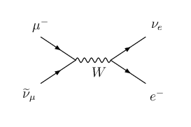
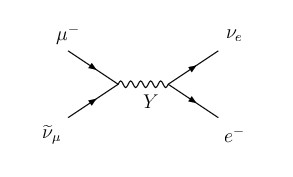
Since one of the VEVs is closely to the those in the standard model: v≃vw​e​a​k=246v\simeq v_{weak}=246 GeV, therefore only two free VEVs exist in the considering model, namely uu and ω\omega. The bilepton mass limit can be obtained from the “wrong” muon decay

μ−→e−​νe​ν~μ\mu^{-}\rightarrow e^{-}\nu_{e}\tilde{\nu}_{\mu} (107)

mediated, at the tree level, by both the standard model WW and the singly-charged bilepton YY (see Fig.2). Remind that in the 3-3-1 model with right-handed neutrinos, at the lowest order, this decay is mediated only by the singly-charged bilepton YY. In our case, the second diagram in Fig.2 gives main contribution.
Refer to caption
Refer to caption
Figure 2: Feynman diagram for the wrong muon decay μ−→e−​νe​ν~μ\mu^{-}\rightarrow e^{-}\nu_{e}\tilde{\nu}_{\mu}.

Taking into account of the famous experimental data [3]

Rm​u​o​n≡Γ⁡(μ−→e−​νe​ν~μ)Γ⁡(μ−→e−​ν~e​νμ)<1.2%90 % CLR_{muon}\equiv\frac{\Gamma(\mu^{-}\rightarrow e^{-}\nu_{e}\tilde{\nu}_{\mu})}{\Gamma(\mu^{-}\rightarrow e^{-}\tilde{\nu}_{e}\nu_{\mu})}<1.2\%\hskip 14.22636pt\textrm{90 \% \ CL} (108)

we get the constraint: Rm​u​o​n≃MW4MY4R_{muon}\simeq\frac{M_{W}^{4}}{M_{Y}^{4}}. Therefore, it follows that MY≥230M_{Y}\geq 230 GeV.

However, the stronger bilepton mass bound of 440 GeV has been derived from consideration of experimental limit on lepton-number violating charged lepton decays [46].

In the case of u→0u\rightarrow 0, analyzing the ZZ decay width [20, 47], the Z−Z′Z-Z^{\prime} mixing angle is constrained by −0.0015≤φ≤0.001-0.0015\leq\varphi\leq 0.001. From atomic parity violation in cesium, bounds for mass of the new exotic Z′Z^{\prime} and the Z−Z′Z-Z^{\prime} mixing angles, again in the limit u→0u\rightarrow 0, are given [20, 47]

−0.00156≤φ≤0.00105,MZ2≥2.1​TeV-0.00156\leq\varphi\leq 0.00105,\hskip 14.22636ptM_{Z_{2}}\geq 2.1\ \textrm{TeV} (109)

These values coincide with the bounds in the usual 3-3-1 model with right-handed neutrinos [48]. The interested reader can find in [23] for the general case u≠0u\neq 0 of the constraints.

For our purpose we consider the ρ\rho parameter - one of the most important quantities of the standard model, having a leading contribution in terms of the TT parameter, is very useful to get the new-physics effects. It is well-known relation between ρ\rho and TT parameter

ρ=1+α​T\rho=1+\alpha T (110)

In the usual 3-3-1 model with right-handed neutrinos, TT gets contribution from the oblique correction and the Z−Z′Z-Z^{\prime} mixing [41]

TR​H​N\displaystyle T_{RHN} =\displaystyle= TZ​Z′+To​b​l​i​q​u​e,\displaystyle T_{ZZ^{\prime}}+T_{oblique}, (111)

where TZ​Z′≃tan2⁡φα​(MZ22MZ12−1)T_{ZZ^{\prime}}\simeq\frac{\tan^{2}\varphi}{\alpha}\left(\frac{M^{2}_{Z_{2}}}{M^{2}_{Z_{1}}}-1\right) is negligible for MZ′M_{Z^{\prime}} less than 1 TeV, To​b​l​i​q​u​eT_{oblique} depends on masses of the top quark and the standard model Higgs boson. Again at the tree level and the limit (27), from (45) and (86) we get an expression for the ρ\rho parameter in the considering model

ρ=MW2cW2​MZ12=v2v2−3​u2≃1+3​u2v2.\rho=\frac{M^{2}_{W}}{c^{2}_{W}M^{2}_{Z^{1}}}=\frac{v^{2}}{v^{2}-3u^{2}}\simeq 1+\frac{3u^{2}}{v^{2}}. (112)

Note that formula (112) has only one free parameter uu, since vv is very close to the VEV in the standard model. Neglecting the contribution from the usual 3-3-1 model with right-handed neutrinos and taking into account the experimental data [3] ρ=0.9987±0.0016\rho=0.9987\pm 0.0016 we get the constraint on uu parameter by uv≤0.01\frac{u}{v}\leq 0.01 which leads to u≤2.46u\leq 2.46 GeV. This means that uu is much smaller than vv, as expected.

It seems that the ρ\rho parameter, at the tree level, in this model, is favorable to be bigger than one and this is similar to the case of the models contained heavy Z′Z^{\prime} [49].

The interesting new physics compared with other 3-3-1 models is the neutrino physics. Due to lepton-number violating couplings we have the following interesting consequences:

  1. 1.

    Processes with Δ​L=±2\Delta L=\pm 2
    From the charged currents we have the following lepton-number violating Δ​L=±2\Delta L=\pm 2 decays such as

    μ−\displaystyle\mu^{-} →\displaystyle\rightarrow e−​νe​νμ,\displaystyle e^{-}\nu_{e}\nu_{\mu},
    μ−\displaystyle\mu^{-} →\displaystyle\rightarrow e−​ν~e​ν~μ,(μ​can be replaced by ​τ)\displaystyle e^{-}\tilde{\nu}_{e}\tilde{\nu}_{\mu},\hskip 14.22636pt(\mu\ \textrm{can be replaced by }\ \tau) (113)

    in which both the standard model WW boson and charged bilepton Yμ−Y_{\mu}^{-} are in intermediate states (see Fig. 3).

    Refer to caption
    Refer to caption
    Figure 3: Feynman diagram for μ−→e−​νe​νμ\mu^{-}\rightarrow e^{-}\nu_{e}\nu_{\mu}.

    Here the main contribution arises from the first diagram. Note that the wrong muon decay violates only family lepton-number, i.e. Δ​L=0\Delta L=0, but not lepton-number at all as in (113). The decay rates are given by

    Rr​a​r​e\displaystyle R_{rare} ≡\displaystyle\equiv Γ⁡(μ−→e−​νe​νμ)Γ⁡(μ−→e−​ν~e​νμ)=Γ⁡(μ−→e−​ν~e​ν~μ)Γ⁡(μ−→e−​ν~e​νμ)≃sθ2.\displaystyle\frac{\Gamma(\mu^{-}\rightarrow e^{-}\nu_{e}\nu_{\mu})}{\Gamma(\mu^{-}\rightarrow e^{-}\tilde{\nu}_{e}\nu_{\mu})}=\frac{\Gamma(\mu^{-}\rightarrow e^{-}\tilde{\nu}_{e}\tilde{\nu}_{\mu})}{\Gamma(\mu^{-}\rightarrow e^{-}\tilde{\nu}_{e}\nu_{\mu})}\simeq s_{\theta}^{2}. (114)

    Taking sθ=0.08s_{\theta}=0.08, we get Rr​a​r​e≃6×10⁻³R_{rare}\simeq 6\times 10^{-3}. This rate is the same as the wrong muon decay one. Interesting to note that, the family lepton-number violating processes

    νi​νi→νj​νj,(i≠j)\nu_{i}\nu_{i}\rightarrow\nu_{j}\nu_{j},\ (i\neq j) (115)

    are mediated not only by the non-Hermitian bilepton XX but also by the Hermitian neutral Z1,Z2Z^{1},Z^{2} (see Fig.4).

    Refer to caption
    Figure 4: Feynman diagram for νiνi→νjνj(i≠j=e,μ,τ)\nu_{i}\nu_{i}\rightarrow\nu_{j}\nu_{j}\hskip 14.22636pt(i\neq j=e,\mu,\tau).

    The first diagram in Fig.4 exists also in the 3-3-1 model with right-handed neutrinos, but the second one does not appear there.

  2. 2.

    Lepton-number violating kaon decays
    Next, let us consider the lepton-number violating decay [3]

    K+→π0+e+​ν~e<3×10⁻³​at​ 90%​CLK^{+}\rightarrow\pi^{0}+e^{+}\tilde{\nu}_{e}\ <3\times 10^{-3}\ \textrm{at}\ 90\%\ \textrm{CL} (116)

    This decay can be explained in the considering model as the subprocess given below

    s~→u~+e+​ν~e.\tilde{s}\rightarrow\tilde{u}+e^{+}\tilde{\nu}_{e}. (117)

    This process is mediated by the standard model WW boson and the charged bilepton YY. Amplitude of the considered process is proportional to sin⁡θ\sin\theta

    M⁡(s~→u~+e+​ν~e)≃sin⁡2​θ2​MW2​(1−MW2MY2)M(\tilde{s}\rightarrow\tilde{u}+e^{+}\tilde{\nu}_{e})\simeq\frac{\sin 2\theta}{2M_{W}^{2}}\left(1-\frac{M_{W}^{2}}{M_{Y}^{2}}\right) (118)

    Next, let us consider the “normal decay” [3]

    K+→π0+e+​νe(4.87±0.06)%K^{+}\rightarrow\pi^{0}+e^{+}\nu_{e}\ \ (4.87\pm 0.06)\ \% (119)

    with amplitude

    M⁡(s~→u~+e+​νe)≃1MW2M(\tilde{s}\rightarrow\tilde{u}+e^{+}\nu_{e})\simeq\frac{1}{M_{W}^{2}} (120)

    From (118) and (120) we get

    Rk​a​o​n≡Γ⁡(s~→u~+e+​ν~e)Γ⁡(s~→u~+e+​νe)≃sin2⁡θ.R_{kaon}\equiv\frac{\Gamma(\tilde{s}\rightarrow\tilde{u}+e^{+}\tilde{\nu}_{e})}{\Gamma(\tilde{s}\rightarrow\tilde{u}+e^{+}\nu_{e})}\simeq\sin^{2}\theta. (121)

    In the framework of this model, we derive the following decay modes with rates

    Rk​a​o​n=Γ⁡(K+→π0+e+​ν~e)Γ⁡(K+→π0+e+​νe)≃Γ⁡(K+→π0+μ+​ν~μ)Γ⁡(K+→π0+μ+​νμ)≃sin2⁡θ≤6×10−3.R_{kaon}=\frac{\Gamma(K^{+}\rightarrow\pi^{0}+e^{+}\tilde{\nu}_{e})}{\Gamma(K^{+}\rightarrow\pi^{0}+e^{+}\nu_{e})}\simeq\frac{\Gamma(K^{+}\rightarrow\pi^{0}+\mu^{+}\tilde{\nu}_{\mu})}{\Gamma(K^{+}\rightarrow\pi^{0}+\mu^{+}\nu_{\mu})}\simeq\sin^{2}\theta\leq 6\times 10^{-3}. (122)

    Note that the similar lepton-number violating processes exist in the SU​(2)R\textrm{SU}(2)_{R} ⊗SU​(2)L⊗U​(1)B−L\otimes\textrm{SU}(2)_{L}\otimes\textrm{U}(1)_{B-L} model (for details, see Ref.[43]).

2.5 Summary

In this section we have presented the 3-3-1 model with the minimal scalar sector (only two Higgs triplets). This version belongs to the 3-3-1 model without exotic charges (charges of the exotic quarks are 23\frac{2}{3} and −13-\frac{1}{3}). The spontaneous symmetry breakdown is achieved with only two Higgs triplets. One of the VEVs uu is a source of lepton-number violations and a reason for the mixing between the charged gauge bosons - the standard model WW and the singly-charged bilepton gauge bosons as well as between neutral non-Hermitian X0X^{0} and neutral gauge bosons: the ZZ and the new exotic Z′Z^{\prime}. At the tree level, masses of the charged gauge bosons satisfy the law of Pythagoras MY2=MX2+MW2M_{Y}^{2}=M_{X}^{2}+M_{W}^{2} and in the limit ω≫u,v\omega\gg u,v, the ρ\rho parameter gets additional contribution dependent only on uv\frac{u}{v}. Thus, this leads to u≪vu\ll v, and there are three quite different scales for the VEVs of the model: one is very small u≃​O​(1)u\simeq\emph{O}(1) GeV - a lepton-number violating parameter, the second vv is close to the standard model one : v≃vw​e​a​k=246v\simeq v_{weak}=246 GeV and the last is in the range of new physics scale about ​O​(1)\emph{O}(1) TeV.

In difference with the usual 3-3-1 model with right-handed neutrinos, in this model the first family of quarks should be distinctive of the two others.

The exact diagonalization of the neutral gauge boson sector is derived. Because of the parameter uu, the lepton-number violation happens only in neutrino but not in charged lepton sector. It is interesting to note that despite the mentioned above mixing, the electromagnetic current remains unchanged. In this model, the lepton-number changing (Δ​L=±2\Delta L=\pm 2) processes exist but only in the neutrino sector.

It is worth mentioning on the advantage of the considered model: the new mixing angle between the charged gauge bosons θ\theta is connected with one of the VEVs uu - the parameter of lepton-number violations. There is no new parameter, but it contains very simple Higgs sector, hence the significant number of free parameters is reduced.

The model contains new kinds of interactions in the neutrino sector. Hence neutrino physics in this model is very rich. We will turn to further studies on neutrino masses and mixing in Section 4.

3 Higgs-Gauge Boson Interactions

We first obtain the scalar fields and mass spectra. The couplings of the scalar fields with the ordinary gauge bosons are presented then. Cross section for the production of the charged Higgs boson at LHC are calculated.

3.1 Higgs Potential

The Higgs potential in the model under consideration is given by Eq. (30). Let us first shift the Higgs fields into physical ones:

χ=(χ1P​0+u2χ2−χ3P​0+ω2),ϕ=(ϕ1+ϕ2P​0+v2ϕ3+).\chi=\left(\begin{array}[]{c}\chi^{P0}_{1}+\frac{u}{\sqrt{2}}\\ \chi^{-}_{2}\\ \chi^{P0}_{3}+\frac{\omega}{\sqrt{2}}\\ \end{array}\right),\hskip 14.22636pt\phi=\left(\begin{array}[]{c}\phi^{+}_{1}\\ \phi^{P0}_{2}+\frac{v}{\sqrt{2}}\\ \phi^{+}_{3}\\ \end{array}\right). (123)

The subscript PP denotes physical fields as in the usual treatment. However, in the following, this subscript will be dropped. By substitution of (123) into (30), the potential becomes

V(χ,ϕ)=μ12[(χ10∗+u2)(χ10+u2)+χ2+χ2−+(χ30∗+ω2)(χ30+ω2)]V(\chi,\phi)=\mu_{1}^{2}\left[\left(\chi^{0*}_{1}+\frac{u}{\sqrt{2}}\right)\left(\chi^{0}_{1}+\frac{u}{\sqrt{2}}\right)+\chi_{2}^{+}\chi_{2}^{-}+\left(\chi^{0*}_{3}+\frac{\omega}{\sqrt{2}}\right)\left(\chi^{0}_{3}+\frac{\omega}{\sqrt{2}}\right)\right]
+μ22[ϕ1−ϕ1++(ϕ20∗+v2)(ϕ20+v2)+ϕ3−ϕ3+]+\mu_{2}^{2}\left[\phi_{1}^{-}\phi_{1}^{+}+\left(\phi^{0*}_{2}+\frac{v}{\sqrt{2}}\right)\left(\phi^{0}_{2}+\frac{v}{\sqrt{2}}\right)+\phi_{3}^{-}\phi_{3}^{+}\right]
+λ1[(χ10∗+u2)(χ10+u2)+χ2+χ2−+(χ30∗+ω2)(χ30+ω2)]2+\lambda_{1}\left[\left(\chi^{0*}_{1}+\frac{u}{\sqrt{2}}\right)\left(\chi^{0}_{1}+\frac{u}{\sqrt{2}}\right)+\chi_{2}^{+}\chi_{2}^{-}+\left(\chi^{0*}_{3}+\frac{\omega}{\sqrt{2}}\right)\left(\chi^{0}_{3}+\frac{\omega}{\sqrt{2}}\right)\right]^{2}
+λ2[ϕ1−ϕ1++(ϕ20∗+v2)(ϕ20+v2)+ϕ3−ϕ3+]2\displaystyle+\lambda_{2}\left[\phi_{1}^{-}\phi_{1}^{+}+\left(\phi^{0*}_{2}+\frac{v}{\sqrt{2}}\right)\left(\phi^{0}_{2}+\frac{v}{\sqrt{2}}\right)+\phi_{3}^{-}\phi_{3}^{+}\right]^{2}
+λ3[(χ10∗+u2)(χ10+u2)+χ2+χ2−+(χ30∗+ω2)(χ30+ω2)]\displaystyle+\lambda_{3}\left[\left(\chi^{0*}_{1}+\frac{u}{\sqrt{2}}\right)\left(\chi^{0}_{1}+\frac{u}{\sqrt{2}}\right)+\chi_{2}^{+}\chi_{2}^{-}+\left(\chi^{0*}_{3}+\frac{\omega}{\sqrt{2}}\right)\left(\chi^{0}_{3}+\frac{\omega}{\sqrt{2}}\right)\right]
×[ϕ1−ϕ1++(ϕ20∗+v2)(ϕ20+v2)+ϕ3−ϕ3+]\displaystyle\times\left[\phi_{1}^{-}\phi_{1}^{+}+\left(\phi^{0*}_{2}+\frac{v}{\sqrt{2}}\right)\left(\phi^{0}_{2}+\frac{v}{\sqrt{2}}\right)+\phi_{3}^{-}\phi_{3}^{+}\right]
+λ4[(χ10∗+u2)ϕ1++χ2+(ϕ20+v2)+(χ30∗+ω2)ϕ3+]\displaystyle+\lambda_{4}\left[\left(\chi^{0*}_{1}+\frac{u}{\sqrt{2}}\right)\phi_{1}^{+}+\chi_{2}^{+}\left(\phi^{0}_{2}+\frac{v}{\sqrt{2}}\right)+\left(\chi^{0*}_{3}+\frac{\omega}{\sqrt{2}}\right)\phi_{3}^{+}\right]
×[ϕ1−(χ10+u2)+(ϕ20∗+v2)χ2−+ϕ3−(χ30+ω2)].\displaystyle\times\left[\phi_{1}^{-}\left(\chi^{0}_{1}+\frac{u}{\sqrt{2}}\right)+\left(\phi^{0*}_{2}+\frac{v}{\sqrt{2}}\right)\chi_{2}^{-}+\phi_{3}^{-}\left(\chi^{0}_{3}+\frac{\omega}{\sqrt{2}}\right)\right]. (124)

From the above expression, we get constraint equations at the tree level

μ12+λ1​(u2+ω2)+λ3​v22\displaystyle\mu_{1}^{2}+\lambda_{1}(u^{2}+\omega^{2})+\lambda_{3}\frac{v^{2}}{2} =\displaystyle= 0,\displaystyle 0, (125)
μ22+λ2​v2+λ3​(u2+ω2)2\displaystyle\mu_{2}^{2}+\lambda_{2}v^{2}+\lambda_{3}\frac{(u^{2}+\omega^{2})}{2} =\displaystyle= 0.\displaystyle 0. (126)

The nonzero values of χ\chi and ϕ\phi at the potential minimum as mentioned can be easily derived from these equations to yield the given (31) and (32).

Since uu is a parameter of lepton-number violation, therefore the terms linear in uu violate the latter. Applying the constraint equations (125) and (126) we get the minimum value, mass terms, lepton-number conserving and violating interactions as follows

V⁡(χ,ϕ)\displaystyle V(\chi,\phi) =\displaystyle= Vmin+VmassN+VmassC+VLNC+VLNV,\displaystyle V_{\mathrm{min}}+V^{\mathrm{N}}_{\mathrm{mass}}+V^{\mathrm{C}}_{\mathrm{mass}}+V_{\mathrm{LNC}}+V_{\mathrm{LNV}}, (127)

where

Vmin\displaystyle V_{\mathrm{min}} =\displaystyle= −λ24​v4−14​(u2+ω2)​[λ1​(u2+ω2)+λ3​v2],\displaystyle-\frac{\lambda_{2}}{4}v^{4}-\frac{1}{4}(u^{2}+\omega^{2})[\lambda_{1}(u^{2}+\omega^{2})+\lambda_{3}v^{2}],
VmassN\displaystyle V^{\mathrm{N}}_{\mathrm{mass}} =\displaystyle= λ1​(u​S1+ω​S3)2+λ2​v2​S22+λ3​v​(u​S1+ω​S3)​S2,\displaystyle\lambda_{1}(uS_{1}+\omega S_{3})^{2}+\lambda_{2}v^{2}S^{2}_{2}+\lambda_{3}v(uS_{1}+\omega S_{3})S_{2}, (128)
VmassC\displaystyle V^{\mathrm{C}}_{\mathrm{mass}} =\displaystyle= λ42​(u​ϕ1++v​χ2++ω​ϕ3+)​(u​ϕ1−+v​χ2−+ω​ϕ3−),\displaystyle\frac{\lambda_{4}}{2}(u\phi^{+}_{1}+v\chi^{+}_{2}+\omega\phi^{+}_{3})(u\phi^{-}_{1}+v\chi^{-}_{2}+\omega\phi^{-}_{3}), (129)
VLNC\displaystyle V_{\mathrm{LNC}} =\displaystyle= λ1​(χ†​χ)2+λ2​(ϕ†​ϕ)2+λ3​(χ†​χ)​(ϕ†​ϕ)+λ4​(χ†​ϕ)​(ϕ†​χ)\displaystyle\lambda_{1}(\chi^{\dagger}\chi)^{2}+\lambda_{2}(\phi^{\dagger}\phi)^{2}+\lambda_{3}(\chi^{\dagger}\chi)(\phi^{\dagger}\phi)+\lambda_{4}(\chi^{\dagger}\phi)(\phi^{\dagger}\chi) (130)
+2​λ1​ω​S3​(χ†​χ)+2​λ2​v​S2​(ϕ†​ϕ)+λ3​v​S2​(χ†​χ)+λ3​ω​S3​(ϕ†​ϕ)\displaystyle+2\lambda_{1}\omega S_{3}(\chi^{\dagger}\chi)+2\lambda_{2}vS_{2}(\phi^{\dagger}\phi)+\lambda_{3}vS_{2}(\chi^{\dagger}\chi)+\lambda_{3}\omega S_{3}(\phi^{\dagger}\phi)
+λ42​(v​χ2−+ω​ϕ3−)​(χ†​ϕ)+λ42​(v​χ2++ω​ϕ3+)​(ϕ†​χ),\displaystyle+\frac{\lambda_{4}}{\sqrt{2}}(v\chi^{-}_{2}+\omega\phi^{-}_{3})(\chi^{\dagger}\phi)+\frac{\lambda_{4}}{\sqrt{2}}(v\chi^{+}_{2}+\omega\phi^{+}_{3})(\phi^{\dagger}\chi),
VLNV\displaystyle V_{\mathrm{LNV}} =\displaystyle= 2​λ1​u​S1​(χ†​χ)+λ3​u​S1​(ϕ†​ϕ)+λ42​u​[ϕ1−​(χ†​ϕ)+ϕ1+​(ϕ†​χ)].\displaystyle 2\lambda_{1}uS_{1}(\chi^{\dagger}\chi)+\lambda_{3}uS_{1}(\phi^{\dagger}\phi)+\frac{\lambda_{4}}{\sqrt{2}}u\left[\phi^{-}_{1}(\chi^{\dagger}\phi)+\phi^{+}_{1}(\phi^{\dagger}\chi)\right]. (131)

In the above equations, we have dropped the subscript PP and used χ=(χ10,χ2−,χ30)T\chi=(\chi^{0}_{1},\chi^{-}_{2},\chi^{0}_{3})^{T}, ϕ=(ϕ1+,ϕ20,ϕ3+)T\phi=(\phi^{+}_{1},\phi^{0}_{2},\phi^{+}_{3})^{T}. Moreover, we have expanded the neutral Higgs fields as

χ10=S1+i​A12,χ30=S3+i​A32,ϕ20=S2+i​A22.\chi^{0}_{1}=\frac{S_{1}+iA_{1}}{\sqrt{2}},\hskip 14.22636pt\chi^{0}_{3}=\frac{S_{3}+iA_{3}}{\sqrt{2}},\hskip 14.22636pt\phi^{0}_{2}=\frac{S_{2}+iA_{2}}{\sqrt{2}}. (132)

In the literature, the real parts (Si,i=1,2,3)(S_{i},i=1,2,3) are also called CP-even scalar and the imaginary part (Ai,i=1,2,3)(A_{i},i=1,2,3) – CP-odd scalar. In this paper, for short, we call them scalar and pseudoscalar field, respectively. As expected, the lepton-number violating part VLNCV_{\mathrm{LNC}} is linear in uu and trilinear in scalar fields. These couplings will be also a source for lepton-number violations such as the mass spectra of quarks including exotic ones as well as neutrino Majorana masses, but given at higher-order corrections.

In the pseudoscalar sector, all the fields are Goldstone bosons: G1=A1G_{1}=A_{1}, G2=A2G_{2}=A_{2} and G3=A3G_{3}=A_{3} (cl. Eq.(128)). The scalar fields S1S_{1}, S2S_{2} and S3S_{3} gain masses via (128), thus we get one Goldstone boson G4G_{4} and two neutral physical fields—the standard model H0H^{0} and the new H10H^{0}_{1} with masses

mH02\displaystyle m^{2}_{H^{0}} =\displaystyle= λ2​v2+λ1​(u2+ω2)−[λ2​v2−λ1​(u2+ω2)]2+λ32​v2​(u2+ω2)\displaystyle\lambda_{2}v^{2}+\lambda_{1}(u^{2}+\omega^{2})-\sqrt{[\lambda_{2}v^{2}-\lambda_{1}(u^{2}+\omega^{2})]^{2}+\lambda^{2}_{3}v^{2}(u^{2}+\omega^{2})} (133)
≃\displaystyle\simeq 4​λ1​λ2−λ322​λ1​v2,\displaystyle\frac{4\lambda_{1}\lambda_{2}-\lambda^{2}_{3}}{2\lambda_{1}}v^{2},
MH102\displaystyle M^{2}_{H^{0}_{1}} =\displaystyle= λ2​v2+λ1​(u2+ω2)+[λ2​v2−λ1​(u2+ω2)]2+λ32​v2​(u2+ω2)\displaystyle\lambda_{2}v^{2}+\lambda_{1}(u^{2}+\omega^{2})+\sqrt{[\lambda_{2}v^{2}-\lambda_{1}(u^{2}+\omega^{2})]^{2}+\lambda^{2}_{3}v^{2}(u^{2}+\omega^{2})} (134)
≃\displaystyle\simeq 2​λ1​ω2.\displaystyle 2\lambda_{1}\omega^{2}.

In term of original fields, the Goldstone and Higgs fields are given by

G4\displaystyle G_{4} =\displaystyle= 11+tθ2​(S1−tθ​S3),\displaystyle\frac{1}{\sqrt{1+t^{2}_{\theta}}}(S_{1}-t_{\theta}S_{3}), (135)
H0\displaystyle H^{0} =\displaystyle= cζ​S2−sζ1+tθ2​(tθ​S1+S3),\displaystyle c_{\zeta}S_{2}-\frac{s_{\zeta}}{\sqrt{1+t^{2}_{\theta}}}(t_{\theta}S_{1}+S_{3}), (136)
H10\displaystyle H^{0}_{1} =\displaystyle= sζ​S2+cζ1+tθ2​(tθ​S1+S3),\displaystyle s_{\zeta}S_{2}+\frac{c_{\zeta}}{\sqrt{1+t^{2}_{\theta}}}(t_{\theta}S_{1}+S_{3}), (137)

where

t2​ζ\displaystyle t_{2\zeta} ≡\displaystyle\equiv λ3​MW​MXλ1​MX2−λ2​MW2.\displaystyle\frac{\lambda_{3}M_{W}M_{X}}{\lambda_{1}M^{2}_{X}-\lambda_{2}M^{2}_{W}}. (138)

From Eq.(134), it follows that mass of the new Higgs boson MH10M_{H^{0}_{1}} is related to mass of the bilepton gauge X0X^{0} (or Y±Y^{\pm} via the law of Pythagoras) through

MH102\displaystyle M^{2}_{H^{0}_{1}} =\displaystyle= 8​λ1g2​MX2​[1+𝒪⁡(MW2MX2)]\displaystyle\frac{8\lambda_{1}}{g^{2}}M_{X}^{2}\left[1+\mathcal{O}\left(\frac{M_{W}^{2}}{M_{X}^{2}}\right)\right] (139)
=\displaystyle= 2​λ1​sW2π​α​MX2​[1+𝒪⁡(MW2MX2)]≈18.8​λ1​MX2.\displaystyle\frac{2\lambda_{1}s^{2}_{W}}{\pi\alpha}M_{X}^{2}\left[1+\mathcal{O}\left(\frac{M_{W}^{2}}{M_{X}^{2}}\right)\right]\approx 18.8\lambda_{1}M_{X}^{2}.

Here, we have used α=1128\alpha=\frac{1}{128} and sW2=0.231s^{2}_{W}=0.231.

In the charged Higgs sector, the mass terms for (ϕ1,χ2,ϕ3)(\phi_{1},\chi_{2},\phi_{3}) are given by (129), thus there are two Goldstone bosons and one physical scalar field:

H2+≡1u2+v2+ω2​(u​ϕ1++v​χ2++ω​ϕ3+)H^{+}_{2}\equiv\frac{1}{\sqrt{u^{2}+v^{2}+\omega^{2}}}(u\phi^{+}_{1}+v\chi^{+}_{2}+\omega\phi^{+}_{3}) (140)

with mass

MH2+2\displaystyle M^{2}_{H^{+}_{2}} =\displaystyle= λ42​(u2+v2+ω2)=2​λ4​MY2g2=sW2​λ42​π​α​MY2≃4.7​λ4​MY2.\displaystyle\frac{\lambda_{4}}{2}(u^{2}+v^{2}+\omega^{2})=2\lambda_{4}\frac{M_{Y}^{2}}{g^{2}}=\frac{s_{W}^{2}\lambda_{4}}{2\pi\alpha}M_{Y}^{2}\simeq 4.7\lambda_{4}M_{Y}^{2}. (141)

The two remaining Goldstone bosons are

G5+\displaystyle G^{+}_{5} =\displaystyle= 11+tθ2​(ϕ1+−tθ​ϕ3+),\displaystyle\frac{1}{\sqrt{1+t^{2}_{\theta}}}(\phi^{+}_{1}-t_{\theta}\phi^{+}_{3}), (142)
G6+\displaystyle G^{+}_{6} =\displaystyle= 1(1+tθ2)​(u2+v2+ω2)​[v⁡(tθ​ϕ1++ϕ3+)−ω⁡(1+tθ2)​χ2+].\displaystyle\frac{1}{\sqrt{(1+t^{2}_{\theta})(u^{2}+v^{2}+\omega^{2})}}\left[v(t_{\theta}\phi^{+}_{1}+\phi^{+}_{3})-\omega(1+t^{2}_{\theta})\chi^{+}_{2}\right]. (143)

Thus, all the pseudoscalars are eigenstates and massless (Goldstone). Other fields are related to the scalars in the weak basis by the linear transformations:

(H0H10G4)=(−sζ​sθcζ−sζ​cθcζ​sθsζcζ​cθcθ0−sθ)​(S1S2S3),\left(\begin{array}[]{ccc}H^{0}\\ H^{0}_{1}\\ G_{4}\end{array}\right)=\left(\begin{array}[]{ccc}-s_{\zeta}s_{\theta}&c_{\zeta}&-s_{\zeta}c_{\theta}\\ c_{\zeta}s_{\theta}&s_{\zeta}&c_{\zeta}c_{\theta}\\ c_{\theta}&0&-s_{\theta}\end{array}\right)\left(\begin{array}[]{ccc}S_{1}\\ S_{2}\\ S_{3}\end{array}\right), (144)
(H2+G5+G6+)=1ω2+cθ2​v2​(ω​sθv​cθω​cθcθ​ω2+cθ2​v20−sθ​ω2+cθ2​v2v​s2​θ2−ωv​cθ2)​(ϕ1+χ2+ϕ3+).\left(\begin{array}[]{c}H^{+}_{2}\\ G^{+}_{5}\\ G^{+}_{6}\end{array}\right)=\frac{1}{\sqrt{\omega^{2}+c^{2}_{\theta}v^{2}}}\left(\begin{array}[]{ccc}\omega s_{\theta}&vc_{\theta}&\omega c_{\theta}\\ c_{\theta}\sqrt{\omega^{2}+c^{2}_{\theta}v^{2}}&0&-s_{\theta}\sqrt{\omega^{2}+c^{2}_{\theta}v^{2}}\\ \frac{vs_{2\theta}}{2}&-\omega&vc^{2}_{\theta}\end{array}\right)\left(\begin{array}[]{c}\phi^{+}_{1}\\ \chi^{+}_{2}\\ \phi^{+}_{3}\end{array}\right). (145)

With the two Higgs triplets of the model, there are twelve real scalar components. Eight of the gauge symmetries of SU​(3)L⊗U​(1)X\mathrm{SU}(3)_{L}\otimes\mathrm{U}(1)_{X} are spontaneously broken, which eliminates just eight Goldstone bosons associated with these fields. It leaves over just four massive scalar particles as obtained (one charged and two natural). There is no Majoron field in this model which contrasts to the 3-3-1 model with right-handed neutrinos [50]. Let us remind the reader that among the Goldstone bosons there are four fields carrying the lepton number but they can be gauged away by an unitary transformation [40].

From (133) and (134), we come to the previous result in Ref.[19]

λ1>0,λ2>0,4​λ1​λ2>λ32.\lambda_{1}>0,\ \lambda_{2}>0,\hskip 14.22636pt4\lambda_{1}\lambda_{2}>\lambda_{3}^{2}. (146)

Eq.(141) shows that the mass of the charged Higgs boson H2±H^{\pm}_{2} is proportional to those of the charged bilepton YY through a coefficient of Higgs self-interaction λ4>0\lambda_{4}>0. Analogously, this happens for the standard-model-like Higgs boson H0H^{0} (MH0∼MW)(M_{H^{0}}\sim M_{W}) and the new H10H^{0}_{1} (MH10∼MX)(M_{H^{0}_{1}}\sim M_{X}). Combining (146) with the constraint equations (125), (126) we get a consequence: λ3\lambda_{3} is negative (λ3<0\lambda_{3}<0). Let us remind the reader that the couplings λ4,1,2\lambda_{4,1,2} are fixed by the Higgs boson masses and λ3\lambda_{3}, where the λ3\lambda_{3} defines the splitting Δ​mH2≃−[λ32/(2​λ1)]​v2\Delta m^{2}_{H}\simeq-[\lambda^{2}_{3}/(2\lambda_{1})]v^{2} from the standard model prediction.

To finish this section, let us comment on our physical Higgs bosons. In the effective approximation w≫v,uw\gg v,u, from Eqs (144), and (145) it follows that

H0\displaystyle H^{0} ∼\displaystyle\sim S2,H10∼S3,G4∼S1,\displaystyle S_{2},\hskip 14.22636ptH_{1}^{0}\sim S_{3},\hskip 14.22636ptG_{4}\sim S_{1},
H2+\displaystyle H^{+}_{2} ∼\displaystyle\sim ϕ3+,G5+∼ϕ1+,G6+∼χ2+.\displaystyle\phi_{3}^{+},\hskip 14.22636ptG^{+}_{5}\sim\phi^{+}_{1},\hskip 14.22636ptG^{+}_{6}\sim\chi^{+}_{2}. (147)

This means that, in the effective approximation, the charged boson H2−H^{-}_{2} is a scalar bilepton (with lepton number L=2L=2), while the neutral scalar bosons H0H^{0} and H10H^{0}_{1} do not carry lepton number (with L=0L=0).

3.2 Higgs–Standard Model Gauge Couplings

There are a total of 9 gauge bosons in the SU​(3)L⊗U​(1)X\mathrm{SU}(3)_{L}\otimes{\mathrm{U}}(1)_{X} group and 8 of them are massive. As shown in the previous section, we have got just 8 massless Goldstone bosons—the justified number for the model. One of the neutral scalars is identified with the standard model Higgs boson, therefore its couplings to ordinary gauge bosons such as the photon, the ZZ and the W±W^{\pm} bosons have to have, in the effective limit, usual known forms. To search Higgs bosons at future high energy colliders, one needs their couplings with ordinary particles, specially with the gauge bosons in the standard model.

The interactions among the gauge bosons and the Higgs bosons arise in part from

∑Y=χ,ϕ(Dμ​Y)†​(Dμ​Y).\sum_{Y=\chi,\ \phi}\left(D_{\mu}Y\right)^{\dagger}\left(D^{\mu}Y\right).

In the following the summation over ​Y\emph{Y} is default and only the terms giving interested couplings are explicitly displayed. The covariant derivative is given by Eq. (33),

Dμ=∂μ−i𝒫μ≡∂μ−i𝒫NCμ−i𝒫μCC,D_{\mu}=\partial_{\mu}-i\mathcal{P}_{\mu}\equiv\partial_{\mu}-i\mathcal{P}^{\mathrm{NC}}_{\mu}-i\mathcal{P}_{\mu}^{\mathrm{CC}}, (148)

where the matrices 𝒫μNC\mathcal{P}^{\mathrm{NC}}_{\mu} and 𝒫μCC\mathcal{P}^{\mathrm{CC}}_{\mu} are written as

𝒫μNC=g2​(W3​μ+W8​μ3+t​23​X​Bμ0yμ0−W3​μ+W8​μ3+t​23​X​Bμ0yμ0−2​W8​μ3+t​23​X​Bμ)\mathcal{P}_{\mu}^{\mathrm{NC}}=\frac{g}{2}\left(\begin{array}[]{ccc}W_{3\mu}+\frac{W_{8\mu}}{\sqrt{3}}+t\sqrt{\frac{2}{3}}XB_{\mu}&0&y_{\mu}\\ 0&-W_{3\mu}+\frac{W_{8\mu}}{\sqrt{3}}+t\sqrt{\frac{2}{3}}XB_{\mu}&0\\ y_{\mu}&0&-\frac{2W_{8\mu}}{\sqrt{3}}+t\sqrt{\frac{2}{3}}XB_{\mu}\\ \end{array}\right) (149)

and

𝒫μCC=g2​(0cθ​Wμ++sθ​Yμ+Xμ0cθ​Wμ−+sθ​Yμ−0cθ​Yμ−−sθ​Wμ−X0∗μcθ​Yμ+−sθ​Wμ+0).\mathcal{P}_{\mu}^{\mathrm{CC}}=\frac{g}{\sqrt{2}}\left(\begin{array}[]{ccc}0&c_{\theta}W^{+}_{\mu}+s_{\theta}Y_{\mu}^{+}&X^{0}_{\mu}\\ c_{\theta}W^{-}_{\mu}+s_{\theta}Y_{\mu}^{-}&0&c_{\theta}Y^{-}_{\mu}-s_{\theta}W_{\mu}^{-}\\ X^{0*}_{\mu}&c_{\theta}Y^{+}_{\mu}-s_{\theta}W_{\mu}^{+}&0\\ \end{array}\right). (150)

Let us recall that t=gX/g=3​2​sW/3−4​sW2t=g_{X}/g=3\sqrt{2}s_{W}/\sqrt{3-4s_{W}^{2}}, tan⁡θ=u/ω\tan\theta=u/\omega, and Wμ±,Yμ±W^{\pm}_{\mu},Y_{\mu}^{\pm} and Xμ0X^{0}_{\mu} are the physical fields. The existence of yμy^{\mu} is a consequence of mixing among the real part (Xμ0∗+Xμ0)(X^{0*}_{\mu}+X^{0}_{\mu}) with W3​μ,W8​μW_{3\mu},W_{8\mu} and BμB_{\mu}; and its expression is determined from the mixing matrix UU given in Appendix A.1:

yμ\displaystyle y_{\mu} ≡\displaystyle\equiv U42​Zμ+U43​Zμ′+(U44−1)​(X0∗μ+X0μ)2,\displaystyle U_{42}Z_{\mu}+U_{43}Z^{\prime}_{\mu}+(U_{44}-1)\frac{(X^{0*}_{\mu}+X^{0}_{\mu})}{\sqrt{2}}, (151)

where

U42\displaystyle U_{42} =\displaystyle= −tθ′​(cφ​1−4​sθ′2​cW2−sφ​4​cW2−1),\displaystyle-t_{\theta^{\prime}}\left(c_{\varphi}\sqrt{1-4s^{2}_{\theta^{\prime}}c^{2}_{W}}-s_{\varphi}\sqrt{4c^{2}_{W}-1}\right),
U43\displaystyle U_{43} =\displaystyle= −tθ′​(sφ​1−4​sθ′2​cW2+cφ​4​cW2−1),\displaystyle-t_{\theta^{\prime}}\left(s_{\varphi}\sqrt{1-4s^{2}_{\theta^{\prime}}c^{2}_{W}}+c_{\varphi}\sqrt{4c^{2}_{W}-1}\right), (152)
U44\displaystyle U_{44} =\displaystyle= 1−4​sθ′2​cW2.\displaystyle\sqrt{1-4s^{2}_{\theta^{\prime}}c^{2}_{W}}.

First, we consider the relevant couplings of the standard model WW boson with the Higgs and Goldstone bosons. The trilinear couplings of the pair W+​W−W^{+}W^{-} with the neutral scalars are given by

(𝒫μCC​⟨χ⟩)†​(𝒫CC​μ​χ)+(𝒫μCC​⟨ϕ⟩)†​(𝒫CC​μ​ϕ)+H.c.=g2​v2​Wμ+​W−μ​S2.(\mathcal{P}^{\mathrm{CC}}_{\mu}\langle\chi\rangle)^{\dagger}(\mathcal{P}^{\mathrm{CC}\mu}\chi)+(\mathcal{P}^{\mathrm{CC}}_{\mu}\langle\phi\rangle)^{\dagger}(\mathcal{P}^{\mathrm{CC}\mu}\phi)+\mathrm{H.c.}=\frac{g^{2}v}{2}W^{+}_{\mu}W^{-\mu}S_{2}. (153)

Because of S2S_{2} is a combination of only HH and H10H_{1}^{0}, therefore, there are two couplings which are given in Table 5.

Table 5: Trilinear coupling constants of W+​W−W^{+}W^{-} with neutral Higgs bosons.
Vertex Coupling
W+​W−​HW^{+}W^{-}H g22​v​cζ\frac{g^{2}}{2}vc_{\zeta}
W+​W−​H10W^{+}W^{-}H_{1}^{0} g22​v​sζ\frac{g^{2}}{2}vs_{\zeta}

Couplings of the single WW with two Higgs bosons exist in

i⁡(Y†​𝒫μCC​∂μY−∂μY†​𝒫μCC​Y)\displaystyle i\left(Y^{\dagger}\mathcal{P}_{\mu}^{\mathrm{CC}}\partial^{\mu}Y-\partial^{\mu}Y^{\dagger}\mathcal{P}_{\mu}^{\mathrm{CC}}Y\right) =\displaystyle= i​g2Wμ−[Y2∗(cθ∂μY1−sθ∂μY3)\displaystyle\frac{ig}{\sqrt{2}}W^{-}_{\mu}\left[Y^{*}_{2}(c_{\theta}\partial^{\mu}Y_{1}-s_{\theta}\partial^{\mu}Y_{3})\right. (154)
−∂μY2∗(cθY1−sθY3)]+H.c.\displaystyle\left.-\partial^{\mu}Y^{*}_{2}(c_{\theta}Y_{1}-s_{\theta}Y_{3})\right]+\mathrm{H.c.}
=\displaystyle= i​g2Wμ−[χ2+(cθ∂μχ10−sθ∂μχ30)−∂μχ2+(cθχ10−sθχ30)\displaystyle\frac{ig}{\sqrt{2}}W^{-}_{\mu}\left[\chi_{2}^{+}(c_{\theta}\partial^{\mu}\chi^{0}_{1}-s_{\theta}\partial^{\mu}\chi^{0}_{3})-\partial^{\mu}\chi_{2}^{+}(c_{\theta}\chi^{0}_{1}-s_{\theta}\chi^{0}_{3})\right. (155)
+\displaystyle+ ϕ20∗(cθ∂μϕ1+−sθ∂μϕ3+)−∂μϕ20∗(cθϕ1+−sθϕ3+)]+H.c.\displaystyle\left.\phi^{0*}_{2}(c_{\theta}\partial^{\mu}\phi^{+}_{1}-s_{\theta}\partial^{\mu}\phi^{+}_{3})-\partial^{\mu}\phi^{0*}_{2}(c_{\theta}\phi^{+}_{1}-s_{\theta}\phi^{+}_{3})\right]+\mathrm{H.c.}

The resulting couplings of the single WW boson with two scalar fields are listed in Table 6,

Table 6: Trilinear coupling constants of W−W^{-} with two Higgs bosons.
Vertex Coupling Vertex Coupling
Wμ−​H2+​∂μ↔​G4W^{\mu-}H^{+}_{2}\overleftrightarrow{\partial_{\mu}}G_{4} i​g​v​cθ2​ω2+cθ2​v2\frac{igvc_{\theta}}{2\sqrt{\omega^{2}+c_{\theta}^{2}v^{2}}} Wμ−​G6+​∂μ↔​G1W^{\mu-}G^{+}_{6}\overleftrightarrow{\partial_{\mu}}G_{1} g​cθ​ω2​ω2+cθ2​v2\frac{gc_{\theta}\omega}{2\sqrt{\omega^{2}+c_{\theta}^{2}v^{2}}}
Wμ−​G5+​∂μ↔​HW^{\mu-}G^{+}_{5}\overleftrightarrow{\partial_{\mu}}H −i​g​cζ2-\frac{igc_{\zeta}}{2} Wμ−​G5+​∂μ↔​G2W^{\mu-}G^{+}_{5}\overleftrightarrow{\partial_{\mu}}G_{2} −g2-\frac{g}{2}
Wμ−​G6+​∂μ↔​G4W^{\mu-}G^{+}_{6}\overleftrightarrow{\partial_{\mu}}G_{4} i​g​ω2​ω2+cθ2​v2\frac{ig\omega}{2\sqrt{\omega^{2}+c_{\theta}^{2}v^{2}}} Wμ−​G5+​∂μ↔​H10W^{\mu-}G^{+}_{5}\overleftrightarrow{\partial_{\mu}}H_{1}^{0} −i​g2​sζ-\frac{ig}{2}s_{\zeta}
Wμ−​H2+​∂μ↔​G1W^{\mu-}H^{+}_{2}\overleftrightarrow{\partial_{\mu}}G_{1} −g​v​cθ22​ω2+cθ2​v2-\frac{gvc^{2}_{\theta}}{2\sqrt{\omega^{2}+c_{\theta}^{2}v^{2}}} Wμ−​G6+​∂μ↔​G30W^{\mu-}G^{+}_{6}\overleftrightarrow{\partial_{\mu}}G^{0}_{3} −g​sθ​ω2​ω2+cθ2​v2-\frac{gs_{\theta}\omega}{2\sqrt{\omega^{2}+c^{2}_{\theta}v^{2}}}
Wμ−​H2+​∂μ↔​G3W^{\mu-}H^{+}_{2}\overleftrightarrow{\partial_{\mu}}G_{3} g​v​s2​θ4​ω2+cθ2​v2\frac{gvs_{2\theta}}{4\sqrt{\omega^{2}+c_{\theta}^{2}v^{2}}}

where we have used a notation A​∂μ↔​B=A⁡(∂μB)−(∂μA)​BA\overleftrightarrow{\partial_{\mu}}B=A(\partial_{\mu}B)-(\partial_{\mu}A)B. Vanishing couplings are

𝒱⁡(W−​H2+​H0)=𝒱⁡(W−​H2+​H10)=𝒱⁡(W−​H0​G6+)\displaystyle\mathcal{V}(W^{-}H^{+}_{2}H^{0})=\mathcal{V}(W^{-}H^{+}_{2}H^{0}_{1})=\mathcal{V}(W^{-}H^{0}G^{+}_{6})
=𝒱⁡(W−​H10​G6+)=𝒱⁡(W−​H2+​G2)=𝒱⁡(W−​G6+​G2)=0.\displaystyle=\mathcal{V}(W^{-}H^{0}_{1}G^{+}_{6})=\mathcal{V}(W^{-}H^{+}_{2}G_{2})=\mathcal{V}(W^{-}G^{+}_{6}G_{2})=0.

Quartic couplings of W+​W−W^{+}W^{-} with two scalar fields arise in part from

(𝒫μCCY)+(𝒫CC​μY)=g22Wμ+W−μ[χ2+χ2−+cθ2χ10∗χ10\displaystyle(\mathcal{P}_{\mu}^{\mathrm{CC}}\emph{Y})^{+}(\mathcal{P}^{\mathrm{CC}\mu}\emph{Y})=\frac{g^{2}}{2}W^{+}_{\mu}W^{-\mu}\left[\chi^{+}_{2}\chi^{-}_{2}+c^{2}_{\theta}\chi^{0*}_{1}\chi^{0}_{1}\right.
+sθ2χ30∗χ30−cθsθ(χ10∗χ30+χ10χ30∗)+ϕ20∗ϕ20\displaystyle+s^{2}_{\theta}\chi^{0*}_{3}\chi^{0}_{3}-c_{\theta}s_{\theta}(\chi^{0*}_{1}\chi^{0}_{3}+\chi^{0}_{1}\chi^{0*}_{3})+\phi^{0*}_{2}\phi^{0}_{2}
+cθ2ϕ1−ϕ1++sθ2ϕ3−ϕ3+−cθsθ(ϕ1+ϕ3−+ϕ1−ϕ3+)].\displaystyle\left.+c^{2}_{\theta}\phi^{-}_{1}\phi^{+}_{1}+s^{2}_{\theta}\phi^{-}_{3}\phi^{+}_{3}-c_{\theta}s_{\theta}(\phi^{+}_{1}\phi^{-}_{3}+\phi^{-}_{1}\phi^{+}_{3})\right]. (156)

With the help of (A.2) and (A.3), we get the interested couplings of W+​W−W^{+}W^{-} with two scalars which are listed in Table 7.

Table 7: Nonzero quartic coupling constants of W+​W−W^{+}W^{-} with Higgs bosons.
Vertex Coupling Vertex Coupling
W+​W−​H2+​H2−W^{+}W^{-}H_{2}^{+}H_{2}^{-} g2​cθ2​v22​(ω2+v2​cθ2)\frac{g^{2}c_{\theta}^{2}v^{2}}{2(\omega^{2}+v^{2}c_{\theta}^{2})} W+​W−​G10​G10W^{+}W^{-}G_{1}^{0}G_{1}^{0} g2​cθ22\frac{g^{2}c_{\theta}^{2}}{2}
W+​W−​G5+​G5−W^{+}W^{-}G_{5}^{+}G_{5}^{-} g22\frac{g^{2}}{2} W+​W−​G30​G30W^{+}W^{-}G_{3}^{0}G_{3}^{0} g2​sθ22\frac{g^{2}s_{\theta}^{2}}{2}
W+​W−​G6+​G6−W^{+}W^{-}G_{6}^{+}G_{6}^{-} g2​ω22​(ω2+cθ2​v2)\frac{g^{2}\omega^{2}}{2(\omega^{2}+c_{\theta}^{2}v^{2})} W+​W−​G40​G40W^{+}W^{-}G_{4}^{0}G_{4}^{0} g22\frac{g^{2}}{2}
W+​W−​H2+​G6−W^{+}W^{-}H_{2}^{+}G_{6}^{-} −g2​cθ​v​ω2​(ω2+cθ2​v2)-\frac{g^{2}c_{\theta}v\omega}{2(\omega^{2}+c_{\theta}^{2}v^{2})} W+​W−​H​H10W^{+}W^{-}HH_{1}^{0} g2​s2​ζ4\frac{g^{2}s_{2\zeta}}{4}
W+​W−​H​HW^{+}W^{-}HH g2​cζ22\frac{g^{2}c^{2}_{\zeta}}{2} W+​W−​G10​G30W^{+}W^{-}G_{1}^{0}G_{3}^{0} −g2​s2​θ4-\frac{g^{2}s_{2\theta}}{4}
W+​W−​H10​H10W^{+}W^{-}H_{1}^{0}H_{1}^{0} g2​sζ22\frac{g^{2}s^{2}_{\zeta}}{2} W+​W−​G20​G20W^{+}W^{-}G^{0}_{2}G^{0}_{2} g22\frac{g^{2}}{2}

Our calculation give following vanishing couplings

𝒱⁡(W+​W−​H2+​G5−)=𝒱⁡(W+​W−​G5+​G6−)\displaystyle\mathcal{V}(W^{+}W^{-}H_{2}^{+}G_{5}^{-})=\mathcal{V}(W^{+}W^{-}G_{5}^{+}G_{6}^{-})
=𝒱⁡(W+​W−​H0​G40)=𝒱⁡(W+​W−​H10​G40)=0.\displaystyle=\mathcal{V}(W^{+}W^{-}H^{0}G_{4}^{0})=\mathcal{V}(W^{+}W^{-}H^{0}_{1}G_{4}^{0})=0. (157)

Now we turn to the couplings of neutral gauge bosons with Higgs bosons. In this case, the interested couplings exist in

i⁡(Y†​𝒫μNC​∂μY−∂μY†​𝒫μNC​Y)\displaystyle i\left(Y^{\dagger}\mathcal{P}_{\mu}^{\mathrm{NC}}\partial^{\mu}Y-\partial^{\mu}Y^{\dagger}\mathcal{P}_{\mu}^{\mathrm{NC}}Y\right) (158)
=\displaystyle= −i​g2{W3μ(∂μχ10∗χ10−∂μχ2+χ2−+∂μϕ1−ϕ1+−∂μϕ20∗ϕ20)\displaystyle-\frac{ig}{2}\left\{W_{3}^{\mu}\left(\partial_{\mu}\chi^{0*}_{1}\chi^{0}_{1}-\partial_{\mu}\chi^{+}_{2}\chi^{-}_{2}+\partial_{\mu}\phi^{-}_{1}\phi^{+}_{1}-\partial_{\mu}\phi^{0*}_{2}\phi^{0}_{2}\right)\right.
+W8μ3(∂μχ10∗χ10+∂μχ2+χ2−+∂μϕ1−ϕ1++∂μϕ20∗ϕ20−2∂μχ30∗χ30−2∂μϕ3−ϕ3+)\displaystyle\left.+\frac{W_{8}^{\mu}}{\sqrt{3}}\left(\partial_{\mu}\chi^{0*}_{1}\chi^{0}_{1}+\partial_{\mu}\chi^{+}_{2}\chi^{-}_{2}+\partial_{\mu}\phi^{-}_{1}\phi^{+}_{1}+\partial_{\mu}\phi^{0*}_{2}\phi^{0}_{2}-2\partial_{\mu}\chi^{0*}_{3}\chi^{0}_{3}-2\partial_{\mu}\phi^{-}_{3}\phi^{+}_{3}\right)\right.
+t23Bμ[−13(∂μχ10∗χ10+∂μχ2+χ2−+∂μχ30∗χ30)+23(∂μϕ1−ϕ1++∂μϕ20∗ϕ20\displaystyle\left.+t\sqrt{\frac{2}{3}}B^{\mu}\left[-\frac{1}{3}\left(\partial_{\mu}\chi^{0*}_{1}\chi^{0}_{1}+\partial_{\mu}\chi^{+}_{2}\chi^{-}_{2}+\partial_{\mu}\chi^{0*}_{3}\chi^{0}_{3}\right)+\frac{2}{3}\left(\partial_{\mu}\phi^{-}_{1}\phi^{+}_{1}+\partial_{\mu}\phi^{0*}_{2}\phi^{0}_{2}\right.\right.\right.
+∂μϕ3−ϕ3+)]+yμ(∂μχ10∗χ30+∂μχ30∗χ10+∂μϕ1−ϕ3++∂μϕ3−ϕ1+)}+H.c.\displaystyle\left.\left.\left.+\partial_{\mu}\phi^{-}_{3}\phi^{+}_{3}\right)\right]+y^{\mu}(\partial_{\mu}\chi^{0*}_{1}\chi^{0}_{3}+\partial_{\mu}\chi^{0*}_{3}\chi^{0}_{1}+\partial_{\mu}\phi^{-}_{1}\phi^{+}_{3}+\partial_{\mu}\phi^{-}_{3}\phi^{+}_{1})\right\}+\mathrm{H.c.}

It can be checked that, as expected, the photon AμA_{\mu} does not interact with neutral Higgs bosons. Other vanishing couplings are

𝒱⁡(A​H2+​G5−)=𝒱⁡(A​H2+​G6−)=𝒱⁡(A​G6+​G5−)=0\displaystyle\mathcal{V}(AH^{+}_{2}G^{-}_{5})=\mathcal{V}(AH^{+}_{2}G^{-}_{6})=\mathcal{V}(AG^{+}_{6}G^{-}_{5})=0 (159)

and

𝒱⁡(A​A​H0)\displaystyle\mathcal{V}(AAH^{0}) =\displaystyle= 𝒱⁡(A​A​H10)=𝒱⁡(A​A​G4)=0,\displaystyle\mathcal{V}(AAH^{0}_{1})=\mathcal{V}(AAG_{4})=0,
𝒱⁡(A​Z​H0)\displaystyle\mathcal{V}(AZH^{0}) =\displaystyle= 𝒱⁡(A​Z​H10)=𝒱⁡(A​Z​G4)=0,\displaystyle\mathcal{V}(AZH^{0}_{1})=\mathcal{V}(AZG_{4})=0,
𝒱⁡(A​Z′​H0)\displaystyle\mathcal{V}(AZ^{\prime}H^{0}) =\displaystyle= 𝒱⁡(A​Z′​H10)=𝒱⁡(A​Z′​G4)=0.\displaystyle\mathcal{V}(AZ^{\prime}H^{0}_{1})=\mathcal{V}(AZ^{\prime}G_{4})=0.

The nonzero electromagnetic couplings are listed in Table 8.

Table 8: Trilinear electromagnetic coupling constants of AμA^{\mu} with two Higgs bosons.
Vertex Aμ​H2−​∂μ↔​H2+A^{\mu}H^{-}_{2}\overleftrightarrow{\partial_{\mu}}H^{+}_{2} Aμ​G5−​∂μ↔​G5+A^{\mu}G^{-}_{5}\overleftrightarrow{\partial_{\mu}}G^{+}_{5} Aμ​G6−​∂μ↔​G6+A^{\mu}G^{-}_{6}\overleftrightarrow{\partial_{\mu}}G^{+}_{6}
Coupling i​eie i​eie i​eie

It should be noticed that the electromagnetic interaction is diagonal, i.e., the non-zero couplings in this model always have a form

i​e​qH​Aμ​H∗​∂μ↔​H.ieq_{H}A^{\mu}H^{*}\overleftrightarrow{\partial_{\mu}}H. (160)

For the ZZ bosons, the following observation is useful

W3μ\displaystyle W_{3}^{\mu} =\displaystyle= U12​Zμ+⋯,W8μ=U22​Zμ+⋯,\displaystyle U_{12}Z^{\mu}+\cdots,\hskip 14.22636ptW_{8}^{\mu}=U_{22}Z^{\mu}+\cdots,
Bμ\displaystyle B^{\mu} =\displaystyle= U32​Zμ+⋯,yμ=U42​Zμ+⋯.\displaystyle U_{32}Z^{\mu}+\cdots,\hskip 14.22636pt\ \ y^{\mu}=U_{42}Z^{\mu}+\cdots. (161)

Here

U12\displaystyle U_{12} =\displaystyle= cφ​cθ′​cW,U22=cφ​(sW2−3​cW2​sθ′2)−sφ​(1−4​sθ′2​cW2)​(4​cW2−1)3​cW​cθ′,\displaystyle c_{\varphi}c_{\theta^{\prime}}c_{W},\hskip 14.22636ptU_{22}=\frac{c_{\varphi}(s^{2}_{W}-3c^{2}_{W}s^{2}_{\theta^{\prime}})-s_{\varphi}\sqrt{(1-4s^{2}_{\theta^{\prime}}c^{2}_{W})(4c^{2}_{W}-1)}}{\sqrt{3}c_{W}c_{\theta^{\prime}}}, (162)
U32\displaystyle U_{32} =\displaystyle= −tW​(cφ​4​cW2−1+sφ​1−4​sθ′2​cW2)3​cθ′\displaystyle-\frac{t_{W}(c_{\varphi}\sqrt{4c^{2}_{W}-1}+s_{\varphi}\sqrt{1-4s^{2}_{\theta^{\prime}}c^{2}_{W}})}{\sqrt{3}c_{\theta^{\prime}}} (163)

are elements in the mixing matrix of the neutral gauge bosons given in Appendix A.1. From (158) and (161), it follows that the trilinear couplings of the single ZZ with charged Higgs bosons exist in part from the Lagrangian terms

−i​g2Zμ[(U12−U223+t323U32)∂μχ2−χ2++(U12+U223+2​t323U32)∂μϕ1−ϕ1+\displaystyle-\frac{ig}{2}Z^{\mu}\left[\left(U_{12}-\frac{U_{22}}{\sqrt{3}}+\frac{t}{3}\sqrt{\frac{2}{3}}U_{32}\right)\partial_{\mu}\chi^{-}_{2}\chi^{+}_{2}+\left(U_{12}+\frac{U_{22}}{\sqrt{3}}+\frac{2t}{3}\sqrt{\frac{2}{3}}U_{32}\right)\partial_{\mu}\phi^{-}_{1}\phi^{+}_{1}\right.
+(−23U22+2​t323U32)∂μϕ3−ϕ3++U42(∂μϕ1−ϕ3++∂μϕ3−ϕ1+)]+H.c.\displaystyle\left.+\left(-\frac{2}{\sqrt{3}}U_{22}+\frac{2t}{3}\sqrt{\frac{2}{3}}U_{32}\right)\partial_{\mu}\phi^{-}_{3}\phi^{+}_{3}+U_{42}\left(\partial_{\mu}\phi^{-}_{1}\phi^{+}_{3}+\partial_{\mu}\phi^{-}_{3}\phi^{+}_{1}\right)\right]+\mathrm{H.c.} (164)

From (164) we get trilinear couplings of the ZZ with the charged Higgs bosons which are listed in Table 9.

Table 9: Trilinear coupling constants of ZμZ^{\mu} with two charged Higgs bosons.
Vertex Coupling
Zμ​H2−​∂μ↔​H2+Z^{\mu}H^{-}_{2}\overleftrightarrow{\partial_{\mu}}H^{+}_{2} i​g2​(ω2+v2​cθ2){(v2cθ2+ω2sθ2)U12+[ω2(1−3cθ2)−v2cθ2]U223\frac{ig}{2(\omega^{2}+v^{2}c_{\theta}^{2})}\left\{(v^{2}c^{2}_{\theta}+\omega^{2}s^{2}_{\theta})U_{12}+[\omega^{2}(1-3c^{2}_{\theta})-v^{2}c^{2}_{\theta}]\frac{U_{22}}{\sqrt{3}}\right.
+(v2cθ2+2ω2)t323U32+ω2s2​θU42}⟶−igsWtW\left.+(v^{2}c^{2}_{\theta}+2\omega^{2})\frac{t}{3}\sqrt{\frac{2}{3}}U_{32}+\omega^{2}s_{2\theta}U_{42}\right\}\longrightarrow-igs_{W}t_{W}
Zμ​G5−​∂μ↔​G5+Z^{\mu}G^{-}_{5}\overleftrightarrow{\partial_{\mu}}G^{+}_{5} i​g2​[cθ2​U12+(1−3​sθ2)​U223+2​t3​23​U32−s2​θ​U42]⟶i​g2​cW​(1−2​sW2)\frac{ig}{2}\left[c^{2}_{\theta}U_{12}+(1-3s^{2}_{\theta})\frac{U_{22}}{\sqrt{3}}+\frac{2t}{3}\sqrt{\frac{2}{3}}U_{32}-s_{2\theta}U_{42}\right]\longrightarrow\frac{ig}{2c_{W}}(1-2s^{2}_{W})
Zμ​G6−​∂μ↔​G6+Z^{\mu}G^{-}_{6}\overleftrightarrow{\partial_{\mu}}G^{+}_{6} i​g2​(ω2+cθ2​v2){(ω2+v2sθ2cθ2)U12+[v2cθ2(1−3cθ2)−ω2]U223\frac{ig}{2(\omega^{2}+c^{2}_{\theta}v^{2})}\left\{(\omega^{2}+v^{2}s^{2}_{\theta}c^{2}_{\theta})U_{12}+[v^{2}c^{2}_{\theta}(1-3c^{2}_{\theta})-\omega^{2}]\frac{U_{22}}{\sqrt{3}}\right.
+t323(ω2+2v2cθ2)U32+2v2sθcθ3U42}⟶i​g2​cW(1−2sW2)\left.+\frac{t}{3}\sqrt{\frac{2}{3}}(\omega^{2}+2v^{2}c^{2}_{\theta})U_{32}+2v^{2}s_{\theta}c^{3}_{\theta}U_{42}\right\}\longrightarrow\frac{ig}{2c_{W}}(1-2s^{2}_{W})
Zμ​H2−​∂μ↔​G5+Z^{\mu}H^{-}_{2}\overleftrightarrow{\partial_{\mu}}G^{+}_{5} i​g​ω4​ω2+cθ2​v2​(s2​θ​U12+3​s2​θ​U22+2​c2​θ​U42)⟶0\frac{ig\omega}{4\sqrt{\omega^{2}+c^{2}_{\theta}v^{2}}}(s_{2\theta}U_{12}+\sqrt{3}s_{2\theta}U_{22}+2c_{2\theta}U_{42})\longrightarrow 0
Zμ​H2−​∂μ↔​G6+Z^{\mu}H^{-}_{2}\overleftrightarrow{\partial_{\mu}}G^{+}_{6} i​g​ω​v​cθ2​(ω2+cθ2​v2)​[−cθ2​U12+(2−3​cθ2)​U223+t3​23​U32+s2​θ​U42]⟶0\frac{ig\omega vc_{\theta}}{2(\omega^{2}+c^{2}_{\theta}v^{2})}\left[-c^{2}_{\theta}U_{12}+(2-3c^{2}_{\theta})\frac{U_{22}}{\sqrt{3}}+\frac{t}{3}\sqrt{\frac{2}{3}}U_{32}+s_{2\theta}U_{42}\right]\longrightarrow 0
Zμ​G5−​∂μ↔​G6+Z^{\mu}G^{-}_{5}\overleftrightarrow{\partial_{\mu}}G^{+}_{6} i​g​v​cθ4​ω2+cθ2​v2​(s2​θ​U12+3​s2​θ​U22+2​c2​θ​U42)⟶0\frac{igvc_{\theta}}{4\sqrt{\omega^{2}+c^{2}_{\theta}v^{2}}}\left(s_{2\theta}U_{12}+\sqrt{3}s_{2\theta}U_{22}+2c_{2\theta}U_{42}\right)\longrightarrow 0

The limit sign (⟶\longrightarrow) in the Tables is the effective one.

In the effective limit, the Z​G5​G5ZG_{5}G_{5} vertex gets an exact expression as in the standard model. Hence G5G_{5} can be identified with the charged Goldstone boson in the standard model (GW+)(G_{W^{+}}).

Now we search couplings of the single ZμZ_{\mu} boson with neutral scalar fields. With the help of the following equations

χ01∂μ↔χ0∗1\displaystyle\chi^{0}_{1}\overleftrightarrow{\partial_{\mu}}\chi^{0*}_{1} =\displaystyle= iG1∂μ↔S1,χ03∂μ↔χ0∗3=iG3∂μ↔S3,ϕ02∂μ↔ϕ0∗2=iG2∂μ↔S2,\displaystyle iG_{1}\overleftrightarrow{\partial_{\mu}}S_{1},\hskip 14.22636pt\chi^{0}_{3}\overleftrightarrow{\partial_{\mu}}\chi^{0*}_{3}=iG_{3}\overleftrightarrow{\partial_{\mu}}S_{3},\hskip 14.22636pt\phi^{0}_{2}\overleftrightarrow{\partial_{\mu}}\phi^{0*}_{2}=iG_{2}\overleftrightarrow{\partial_{\mu}}S_{2},
∂μχ0∗1χ03+∂μχ0∗3χ01\displaystyle\partial_{\mu}\chi^{0*}_{1}\chi^{0}_{3}+\partial_{\mu}\chi^{0*}_{3}\chi^{0}_{1} =\displaystyle= 12[∂μS1S3+∂μS3S1+∂μG1G3+∂μG3G1+iG3∂μ↔S1\displaystyle\frac{1}{2}\left[\partial_{\mu}S_{1}S_{3}+\partial_{\mu}S_{3}S_{1}+\partial_{\mu}G_{1}G_{3}+\partial_{\mu}G_{3}G_{1}+iG_{3}\overleftrightarrow{\partial_{\mu}}S_{1}\right.
+iG1∂μ↔S3],\displaystyle\left.+iG_{1}\overleftrightarrow{\partial_{\mu}}S_{3}\right],

the necessary parts of Lagrangian are

g2[(U12+U223−t323U32)G1∂μ↔S1+U42G1∂μ↔S3+(−23U22−t323U32)\displaystyle\frac{g}{2}\left[\left(U_{12}+\frac{U_{22}}{\sqrt{3}}-\frac{t}{3}\sqrt{\frac{2}{3}}U_{32}\right)G_{1}\overleftrightarrow{\partial_{\mu}}S_{1}+U_{42}G_{1}\overleftrightarrow{\partial_{\mu}}S_{3}+\left(-\frac{2}{\sqrt{3}}U_{22}-\frac{t}{3}\sqrt{\frac{2}{3}}U_{32}\right)\right.
×G3∂μ↔S3+U42G3∂μ↔S1+(−U12+U223+2​t323U32)G2∂μ↔S2].\displaystyle\left.\times G_{3}\overleftrightarrow{\partial_{\mu}}S_{3}+U_{42}G_{3}\overleftrightarrow{\partial_{\mu}}S_{1}+\left(-U_{12}+\frac{U_{22}}{\sqrt{3}}+\frac{2t}{3}\sqrt{\frac{2}{3}}U_{32}\right)G_{2}\overleftrightarrow{\partial_{\mu}}S_{2}\right].

The resulting couplings are listed in Table 10.

Table 10: Trilinear coupling constants of ZμZ_{\mu} with two neutral Higgs bosons.
Vertex Coupling
Zμ​G1​∂μ↔​HZ^{\mu}G_{1}\overleftrightarrow{\partial_{\mu}}H −g​sζ2​[(U12+U223−t3​23​U32)​sθ+U42​cθ]⟶0-\frac{gs_{\zeta}}{2}\left[\left(U_{12}+\frac{U_{22}}{\sqrt{3}}-\frac{t}{3}\sqrt{\frac{2}{3}}U_{32}\right)s_{\theta}+U_{42}c_{\theta}\right]\longrightarrow 0
Zμ​G2​∂μ↔​HZ^{\mu}G_{2}\overleftrightarrow{\partial_{\mu}}H g2​(−U12+U223+2​t3​23​U32)​cζ⟶−g2​cW\frac{g}{2}\left(-U_{12}+\frac{U_{22}}{\sqrt{3}}+\frac{2t}{3}\sqrt{\frac{2}{3}}U_{32}\right)c_{\zeta}\longrightarrow-\frac{g}{2c_{W}}
Zμ​G3​∂μ↔​HZ^{\mu}G_{3}\overleftrightarrow{\partial_{\mu}}H g​sζ2​[(23​U22+t3​23​U32)​cθ−U42​sθ]⟶0\frac{gs_{\zeta}}{2}\left[\left(\frac{2}{\sqrt{3}}U_{22}+\frac{t}{3}\sqrt{\frac{2}{3}}U_{32}\right)c_{\theta}-U_{42}s_{\theta}\right]\longrightarrow 0
Zμ​G1​∂μ↔​H10Z^{\mu}G_{1}\overleftrightarrow{\partial_{\mu}}H^{0}_{1} g​cζ2​[(U12+U223−t3​23​U32)​sθ+U42​cθ]⟶0\frac{gc_{\zeta}}{2}\left[\left(U_{12}+\frac{U_{22}}{\sqrt{3}}-\frac{t}{3}\sqrt{\frac{2}{3}}U_{32}\right)s_{\theta}+U_{42}c_{\theta}\right]\longrightarrow 0
Zμ​G2​∂μ↔​H10Z^{\mu}G_{2}\overleftrightarrow{\partial_{\mu}}H^{0}_{1} g2​(−U12+U223+2​t3​23​U32)​sζ⟶0\frac{g}{2}\left(-U_{12}+\frac{U_{22}}{\sqrt{3}}+\frac{2t}{3}\sqrt{\frac{2}{3}}U_{32}\right)s_{\zeta}\longrightarrow 0
Zμ​G3​∂μ↔​H10Z^{\mu}G_{3}\overleftrightarrow{\partial_{\mu}}H^{0}_{1} −g​cζ2​[(23​U22+t3​23​U32)​cθ−U42​sθ]⟶0-\frac{gc_{\zeta}}{2}\left[\left(\frac{2}{\sqrt{3}}U_{22}+\frac{t}{3}\sqrt{\frac{2}{3}}U_{32}\right)c_{\theta}-U_{42}s_{\theta}\right]\longrightarrow 0
Zμ​G1​∂μ↔​G4Z^{\mu}G_{1}\overleftrightarrow{\partial_{\mu}}G_{4} g2​[(U12+U223−t3​23​U32)​cθ−U42​sθ]⟶g2​cW\frac{g}{2}\left[\left(U_{12}+\frac{U_{22}}{\sqrt{3}}-\frac{t}{3}\sqrt{\frac{2}{3}}U_{32}\right)c_{\theta}-U_{42}s_{\theta}\right]\longrightarrow\frac{g}{2c_{W}}
Zμ​G2​∂μ↔​G4Z^{\mu}G_{2}\overleftrightarrow{\partial_{\mu}}G_{4} 00
Zμ​G3​∂μ↔​G4Z^{\mu}G_{3}\overleftrightarrow{\partial_{\mu}}G_{4} g2​[(23​U22+t3​23​U32)​sθ+U42​cθ]⟶0\frac{g}{2}\left[\left(\frac{2}{\sqrt{3}}U_{22}+\frac{t}{3}\sqrt{\frac{2}{3}}U_{32}\right)s_{\theta}+U_{42}c_{\theta}\right]\longrightarrow 0

From Table 10, we conclude that G2G_{2} should be identified to GZG_{Z} in the standard model. For the Z′Z^{\prime} boson, the following remark is again helpful

W3μ\displaystyle W_{3}^{\mu} =\displaystyle= U13​Zμ′+⋯,W8μ=U23​Zμ′+⋯,\displaystyle U_{13}Z^{{}^{\prime}\mu}+\cdots,\hskip 14.22636ptW_{8}^{\mu}=U_{23}Z^{{}^{\prime}\mu}+\cdots,
Bμ\displaystyle B^{\mu} =\displaystyle= U33​Zμ′+⋯,yμ=U43​Zμ′+⋯,\displaystyle U_{33}Z^{{}^{\prime}\mu}+\cdots,\hskip 14.22636pt\ \ y^{\mu}=U_{43}Z^{{}^{\prime}\mu}+\cdots, (165)

where

U13\displaystyle U_{13} =\displaystyle= sφ​cθ′​cW,U23=sφ​(sW2−3​cW2​sθ′2)+cφ​(1−4​sθ′2​cW2)​(4​cW2−1)3​cW​cθ′,\displaystyle s_{\varphi}c_{\theta^{\prime}}c_{W},\hskip 14.22636ptU_{23}=\frac{s_{\varphi}(s^{2}_{W}-3c^{2}_{W}s^{2}_{\theta^{\prime}})+c_{\varphi}\sqrt{(1-4s^{2}_{\theta^{\prime}}c^{2}_{W})(4c^{2}_{W}-1)}}{\sqrt{3}c_{W}c_{\theta^{\prime}}}, (166)
U33\displaystyle U_{33} =\displaystyle= −tW​(sφ​4​cW2−1−cφ​1−4​sθ′2​cW2)3​cθ′.\displaystyle-\frac{t_{W}(s_{\varphi}\sqrt{4c^{2}_{W}-1}-c_{\varphi}\sqrt{1-4s^{2}_{\theta^{\prime}}c^{2}_{W}})}{\sqrt{3}c_{\theta^{\prime}}}. (167)

Thus, with the replacement Z→Z′Z\rightarrow Z^{\prime} one just replaces column 22 by 33, for example, trilinear coupling constants of the Zμ′Z^{\prime}_{\mu} with two neutral Higgs bosons are given in Table 11.

Table 11: Trilinear coupling constants of Zμ′Z^{\prime}_{\mu} with two neutral Higgs bosons.
Vertex Coupling
Z′μ​G1​∂μ↔​HZ^{\prime\mu}G_{1}\overleftrightarrow{\partial_{\mu}}H −g​sζ2​[(U13+U233−t3​23​U33)​sθ+U43​cθ]⟶0-\frac{gs_{\zeta}}{2}\left[\left(U_{13}+\frac{U_{23}}{\sqrt{3}}-\frac{t}{3}\sqrt{\frac{2}{3}}U_{33}\right)s_{\theta}+U_{43}c_{\theta}\right]\longrightarrow 0
Z′μ​G2​∂μ↔​HZ^{\prime\mu}G_{2}\overleftrightarrow{\partial_{\mu}}H g2​(−U13+U233+2​t3​23​U33)​cζ⟶g2​cW​4​cW2−1\frac{g}{2}\left(-U_{13}+\frac{U_{23}}{\sqrt{3}}+\frac{2t}{3}\sqrt{\frac{2}{3}}U_{33}\right)c_{\zeta}\longrightarrow\frac{g}{2c_{W}\sqrt{4c^{2}_{W}-1}}
Z′μ​G3​∂μ↔​HZ^{\prime\mu}G_{3}\overleftrightarrow{\partial_{\mu}}H g​sζ2​[(23​U23+t3​23​U33)​cθ−U43​sθ]⟶0\frac{gs_{\zeta}}{2}\left[\left(\frac{2}{\sqrt{3}}U_{23}+\frac{t}{3}\sqrt{\frac{2}{3}}U_{33}\right)c_{\theta}-U_{43}s_{\theta}\right]\longrightarrow 0
Z′μ​G1​∂μ↔​H10Z^{\prime\mu}G_{1}\overleftrightarrow{\partial_{\mu}}H^{0}_{1} g​cζ2​[(U13+U233−t3​23​U33)​sθ+U43​cθ]⟶0\frac{gc_{\zeta}}{2}\left[\left(U_{13}+\frac{U_{23}}{\sqrt{3}}-\frac{t}{3}\sqrt{\frac{2}{3}}U_{33}\right)s_{\theta}+U_{43}c_{\theta}\right]\longrightarrow 0
Z′μ​G2​∂μ↔​H10Z^{\prime\mu}G_{2}\overleftrightarrow{\partial_{\mu}}H^{0}_{1} g2​(−U13+U233+2​t3​23​U33)​sζ⟶0\frac{g}{2}\left(-U_{13}+\frac{U_{23}}{\sqrt{3}}+\frac{2t}{3}\sqrt{\frac{2}{3}}U_{33}\right)s_{\zeta}\longrightarrow 0
Z′μ​G3​∂μ↔​H10Z^{\prime\mu}G_{3}\overleftrightarrow{\partial_{\mu}}H^{0}_{1} −g​cζ2​[(23​U23+t3​23​U33)​cθ−U43​sθ]⟶−g​cW4​cW2−1-\frac{gc_{\zeta}}{2}\left[\left(\frac{2}{\sqrt{3}}U_{23}+\frac{t}{3}\sqrt{\frac{2}{3}}U_{33}\right)c_{\theta}-U_{43}s_{\theta}\right]\longrightarrow-\frac{gc_{W}}{\sqrt{4c^{2}_{W}-1}}
Z′μ​G1​∂μ↔​G4Z^{\prime\mu}G_{1}\overleftrightarrow{\partial_{\mu}}G_{4} g2​[(U13+U233−t3​23​U33)​cθ−U43​sθ]⟶g​c2​W2​cW​4​cW2−1\frac{g}{2}\left[\left(U_{13}+\frac{U_{23}}{\sqrt{3}}-\frac{t}{3}\sqrt{\frac{2}{3}}U_{33}\right)c_{\theta}-U_{43}s_{\theta}\right]\longrightarrow\frac{gc_{2W}}{2c_{W}\sqrt{4c_{W}^{2}-1}}
Z′μ​G2​∂μ↔​G4Z^{\prime\mu}G_{2}\overleftrightarrow{\partial_{\mu}}G_{4} 00
Z′μ​G3​∂μ↔​G4Z^{\prime\mu}G_{3}\overleftrightarrow{\partial_{\mu}}G_{4} g2​[(23​U23+t3​23​U33)​sθ+U43​cθ]⟶0\frac{g}{2}\left[\left(\frac{2}{\sqrt{3}}U_{23}+\frac{t}{3}\sqrt{\frac{2}{3}}U_{33}\right)s_{\theta}+U_{43}c_{\theta}\right]\longrightarrow 0

Next, we search couplings of two neutral gauge bosons with scalar fields which arise in part from

Y+​𝒫μNC​𝒫NC​μ​Y\displaystyle Y^{+}\mathcal{P}^{\mathrm{NC}}_{\mu}\mathcal{P}^{\mathrm{NC}\mu}Y =\displaystyle= g24{[Y1∗(A11μA11​μ+yμyμ)+Y3∗(A11​μyμ+A33​μyμ)]Y1+A22μA22​μ\displaystyle\frac{g^{2}}{4}\left\{\left[Y^{*}_{1}(A_{11}^{\mu}A_{11\mu}+y_{\mu}y^{\mu})+Y^{*}_{3}(A_{11\mu}y^{\mu}+A_{33\mu}y^{\mu})\right]Y_{1}+A_{22}^{\mu}A_{22\mu}\right. (168)
×Y2∗Y2+[Y1∗(A11​μyμ+A33​μyμ)+Y3∗(A33μA33​μ+yμyμ)]Y3},\displaystyle\left.\times Y^{*}_{2}Y_{2}+\left[Y^{*}_{1}(A_{11\mu}y^{\mu}+A_{33\mu}y^{\mu})+Y^{*}_{3}(A_{33}^{\mu}A_{33\mu}+y_{\mu}y^{\mu})\right]Y_{3}\right\},
=\displaystyle= g24{[χ10∗(A11μ​χA11​μχ+yμyμ)+χ30∗(A11​μχyμ+A33​μχyμ)]χ10\displaystyle\frac{g^{2}}{4}\left\{\left[\chi^{0*}_{1}\left(A_{11}^{\mu\chi}A_{11\mu}^{\chi}+y_{\mu}y^{\mu}\right)+\chi^{0*}_{3}\left(A_{11\mu}^{\chi}y^{\mu}+A_{33\mu}^{\chi}y^{\mu}\right)\right]\chi^{0}_{1}\right.
+[χ10∗(A11​μχyμ+A33​μχyμ)+χ30∗(A33μ​χA33​μχ+yμyμ)]χ30\displaystyle+\left[\chi^{0*}_{1}\left(A_{11\mu}^{\chi}y^{\mu}+A_{33\mu}^{\chi}y^{\mu}\right)+\chi^{0*}_{3}\left(A_{33}^{\mu\chi}A_{33\mu}^{\chi}+y_{\mu}y^{\mu}\right)\right]\chi^{0}_{3}
+[ϕ1−​(A11μ​ϕ​A11​μϕ+yμ​yμ)+ϕ3−​(A11​μϕ​yμ+A33​μϕ​yμ)]​ϕ1+\displaystyle+\left[\phi^{-}_{1}\left(A_{11}^{\mu\phi}A_{11\mu}^{\phi}+y_{\mu}y^{\mu}\right)+\phi^{-}_{3}\left(A_{11\mu}^{\phi}y^{\mu}+A_{33\mu}^{\phi}y^{\mu}\right)\right]\phi^{+}_{1}
+[ϕ1−​(A11​μϕ​yμ+A33​μϕ​yμ)+ϕ3−​(A33μ​ϕ​A33​μϕ+yμ​yμ)]​ϕ3+\displaystyle+\left[\phi^{-}_{1}\left(A_{11\mu}^{\phi}y^{\mu}+A_{33\mu}^{\phi}y^{\mu}\right)+\phi^{-}_{3}\left(A_{33}^{\mu\phi}A_{33\mu}^{\phi}+y_{\mu}y^{\mu}\right)\right]\phi^{+}_{3}
+(A22μ​χA22​μχ)χ2+χ2−+(A22μ​ϕA22​μϕ)ϕ20∗ϕ20}.\displaystyle+\left.\left(A_{22}^{\mu\chi}A_{22\mu}^{\chi}\right)\chi^{+}_{2}\chi_{2}^{-}+\left(A_{22}^{\mu\phi}A_{22\mu}^{\phi}\right)\phi^{0*}_{2}\phi^{0}_{2}\right\}.

Here Ai​iμA_{ii}^{\mu} (i=1,2,3)(i=1,2,3) is a diagonal element in the matrix 2g​𝒫μNC\frac{2}{g}\mathcal{P}^{\mathrm{NC}}_{\mu} which is dependent on the U​(1)XU(1)_{X} charge:

A11μ​χ\displaystyle A_{11}^{\mu\chi} =\displaystyle= W3μ+W8μ3−t3​23​Bμ,A11μ​ϕ=W3μ+W8μ3+2​t3​23​Bμ,\displaystyle W_{3}^{\mu}+\frac{W_{8}^{\mu}}{\sqrt{3}}-\frac{t}{3}\sqrt{\frac{2}{3}}B^{\mu},\hskip 14.22636ptA_{11}^{\mu\phi}=W_{3}^{\mu}+\frac{W_{8}^{\mu}}{\sqrt{3}}+\frac{2t}{3}\sqrt{\frac{2}{3}}B^{\mu},
A22μ​χ\displaystyle A_{22}^{\mu\chi} =\displaystyle= −W3μ+W8μ3−t3​23​Bμ,A22μ​ϕ=−W3μ+W8μ3+2​t3​23​Bμ,\displaystyle-W_{3}^{\mu}+\frac{W_{8}^{\mu}}{\sqrt{3}}-\frac{t}{3}\sqrt{\frac{2}{3}}B^{\mu},\hskip 14.22636ptA_{22}^{\mu\phi}=-W_{3}^{\mu}+\frac{W_{8}^{\mu}}{\sqrt{3}}+\frac{2t}{3}\sqrt{\frac{2}{3}}B^{\mu}, (169)
A33μ​χ\displaystyle A_{33}^{\mu\chi} =\displaystyle= −2​W8μ3−t3​23​Bμ,A33μ​ϕ=−2​W8μ3+2​t3​23​Bμ.\displaystyle-2\frac{W_{8}^{\mu}}{\sqrt{3}}-\frac{t}{3}\sqrt{\frac{2}{3}}B^{\mu},\hskip 14.22636ptA_{33}^{\mu\phi}=-2\frac{W_{8}^{\mu}}{\sqrt{3}}+\frac{2t}{3}\sqrt{\frac{2}{3}}B^{\mu}.

Quartic couplings of two ZZ with neutral scalar fields are given by

g24{[χ10∗(A11μ​χA11​μχ+yμyμ)+χ30∗(A11​μχyμ+A33​μχyμ)]χ10\displaystyle\frac{g^{2}}{4}\left\{\left[\chi^{0*}_{1}\left(A_{11}^{\mu\chi}A_{11\mu}^{\chi}+y_{\mu}y^{\mu}\right)+\chi^{0*}_{3}\left(A_{11\mu}^{\chi}y^{\mu}+A_{33\mu}^{\chi}y^{\mu}\right)\right]\chi^{0}_{1}\right.
+[χ10∗(A11​μχyμ+A33​μχyμ)+χ30∗(A33μ​χA33​μχ+yμyμ)]χ30+(A22μ​ϕA22​μϕ)ϕ20∗ϕ20}\displaystyle+\left.\left[\chi^{0*}_{1}\left(A_{11\mu}^{\chi}y^{\mu}+A_{33\mu}^{\chi}y^{\mu}\right)+\chi^{0*}_{3}\left(A_{33}^{\mu\chi}A_{33\mu}^{\chi}+y_{\mu}y^{\mu}\right)\right]\chi^{0}_{3}+\left(A_{22}^{\mu\phi}A_{22\mu}^{\phi}\right)\phi^{0*}_{2}\phi^{0}_{2}\right\}
=g24{(A11μ​χA11​μχ+yμyμ)χ10∗χ10+(A33μ​χA33​μχ+yμyμ)χ30∗χ30\displaystyle=\frac{g^{2}}{4}\left\{\left(A_{11}^{\mu\chi}A_{11\mu}^{\chi}+y_{\mu}y^{\mu}\right)\chi^{0*}_{1}\chi^{0}_{1}+\left(A_{33}^{\mu\chi}A_{33\mu}^{\chi}+y_{\mu}y^{\mu}\right)\chi^{0*}_{3}\chi^{0}_{3}\right.
+(A11​μχyμ+A33​μχyμ)(χ10∗χ30+χ30∗χ10)+(A22μ​ϕA22​μϕ)ϕ20∗ϕ20}.\displaystyle\left.+\left(A_{11\mu}^{\chi}y^{\mu}+A_{33\mu}^{\chi}y^{\mu}\right)(\chi^{0*}_{1}\chi^{0}_{3}+\chi^{0*}_{3}\chi^{0}_{1})+\left(A_{22}^{\mu\phi}A_{22\mu}^{\phi}\right)\phi^{0*}_{2}\phi^{0}_{2}\right\}. (170)

In this case, the couplings are listed in Table 12.

Table 12: Quartic coupling constants of Z​ZZZ with two scalar bosons.
Vertex Coupling
Z​Z​G1​G1ZZG_{1}G_{1} g22​[(U12+U223−t3​23​U32)2+U422]⟶g22​cW2\frac{g^{2}}{2}\left[\left(U_{12}+\frac{U_{22}}{\sqrt{3}}-\frac{t}{3}\sqrt{\frac{2}{3}}U_{32}\right)^{2}+U_{42}^{2}\right]\longrightarrow\frac{g^{2}}{2c_{W}^{2}}
Z​Z​G2​G2ZZG_{2}G_{2} g22​(−U12+U223+2​t3​23​U32)2⟶g22​cW2\frac{g^{2}}{2}\left(-U_{12}+\frac{U_{22}}{\sqrt{3}}+\frac{2t}{3}\sqrt{\frac{2}{3}}U_{32}\right)^{2}\longrightarrow\frac{g^{2}}{2c_{W}^{2}}
Z​Z​G3​G3ZZG_{3}G_{3} g22​[(23​U22+t3​23​U32)2+U422]⟶0\frac{g^{2}}{2}\left[\left(\frac{2}{\sqrt{3}}U_{22}+\frac{t}{3}\sqrt{\frac{2}{3}}U_{32}\right)^{2}+U^{2}_{42}\right]\longrightarrow 0
Z​Z​G1​G3ZZG_{1}G_{3} g22​(U12−U223−2​t3​23​U32)​U42⟶0\frac{g^{2}}{2}\left(U_{12}-\frac{U_{22}}{\sqrt{3}}-\frac{2t}{3}\sqrt{\frac{2}{3}}U_{32}\right)U_{42}\longrightarrow 0
Z​Z​H​HZZHH g22{sζ2[sθ2(U12+U223−t323U32)2+cθ2(23U22+t323U32)2+U422\frac{g^{2}}{2}\left\{s^{2}_{\zeta}\left[s^{2}_{\theta}\left(U_{12}+\frac{U_{22}}{\sqrt{3}}-\frac{t}{3}\sqrt{\frac{2}{3}}U_{32}\right)^{2}+c^{2}_{\theta}\left(\frac{2}{\sqrt{3}}U_{22}+\frac{t}{3}\sqrt{\frac{2}{3}}U_{32}\right)^{2}+U_{42}^{2}\right.\right.
+s2​θU42(U12−U223−2​t323U32)]+cζ2(U12−U223−2​t323U32)2}⟶g22​cW2\left.\left.+s_{2\theta}U_{42}\left(U_{12}-\frac{U_{22}}{\sqrt{3}}-\frac{2t}{3}\sqrt{\frac{2}{3}}U_{32}\right)\right]+c^{2}_{\zeta}\left(U_{12}-\frac{U_{22}}{\sqrt{3}}-\frac{2t}{3}\sqrt{\frac{2}{3}}U_{32}\right)^{2}\right\}\longrightarrow\frac{g^{2}}{2c_{W}^{2}}
Z​Z​H10​H10ZZH^{0}_{1}H^{0}_{1} g22{cζ2[sθ2(U12+U223−t323U32)2+cθ2(23U22+t323U32)2+U422\frac{g^{2}}{2}\left\{c^{2}_{\zeta}\left[s^{2}_{\theta}\left(U_{12}+\frac{U_{22}}{\sqrt{3}}-\frac{t}{3}\sqrt{\frac{2}{3}}U_{32}\right)^{2}+c^{2}_{\theta}\left(\frac{2}{\sqrt{3}}U_{22}+\frac{t}{3}\sqrt{\frac{2}{3}}U_{32}\right)^{2}+U_{42}^{2}\right.\right.
+s2​θU42(U12−U223−2​t323U32)]+sζ2(U12−U223−2​t323U32)2}⟶0\left.\left.+s_{2\theta}U_{42}\left(U_{12}-\frac{U_{22}}{\sqrt{3}}-\frac{2t}{3}\sqrt{\frac{2}{3}}U_{32}\right)\right]+s^{2}_{\zeta}\left(U_{12}-\frac{U_{22}}{\sqrt{3}}-\frac{2t}{3}\sqrt{\frac{2}{3}}U_{32}\right)^{2}\right\}\longrightarrow 0
Z​Z​G4​G4ZZG_{4}G_{4} g22[cθ2(U12+U223−t323U32)2+sθ2(23U22+t323U32)2\frac{g^{2}}{2}\left[c^{2}_{\theta}\left(U_{12}+\frac{U_{22}}{\sqrt{3}}-\frac{t}{3}\sqrt{\frac{2}{3}}U_{32}\right)^{2}+s^{2}_{\theta}\left(\frac{2}{\sqrt{3}}U_{22}+\frac{t}{3}\sqrt{\frac{2}{3}}U_{32}\right)^{2}\right.
−s2​θ(U12−U223−2​t323U32)U42+U422]⟶g22​cW2\left.-s_{2\theta}\left(U_{12}-\frac{U_{22}}{\sqrt{3}}-\frac{2t}{3}\sqrt{\frac{2}{3}}U_{32}\right)U_{42}+U_{42}^{2}\right]\longrightarrow\frac{g^{2}}{2c^{2}_{W}}
Z​Z​H​H1ZZHH_{1} −g2​s2​ζ4[sθ2(U12+U223−t323U32)2+cθ2(23U22+t323U32)2+U422-\frac{g^{2}s_{2\zeta}}{4}\left[s^{2}_{\theta}\left(U_{12}+\frac{U_{22}}{\sqrt{3}}-\frac{t}{3}\sqrt{\frac{2}{3}}U_{32}\right)^{2}+c^{2}_{\theta}\left(\frac{2}{\sqrt{3}}U_{22}+\frac{t}{3}\sqrt{\frac{2}{3}}U_{32}\right)^{2}+U_{42}^{2}\right.
−(U12−U223−2​t323U32)2+s2​θ(U12−U223−2​t323U32)U42]⟶0\left.-\left(U_{12}-\frac{U_{22}}{\sqrt{3}}-\frac{2t}{3}\sqrt{\frac{2}{3}}U_{32}\right)^{2}+s_{2\theta}\left(U_{12}-\frac{U_{22}}{\sqrt{3}}-\frac{2t}{3}\sqrt{\frac{2}{3}}U_{32}\right)U_{42}\right]\longrightarrow 0
Z​Z​H​G4ZZHG_{4} −g2​sζ4​(U12−U223−2​t3​23​U32)​[2​c2​θ​U42+s2​θ​(U12+3​U22)]⟶0-\frac{g^{2}s_{\zeta}}{4}\left(U_{12}-\frac{U_{22}}{\sqrt{3}}-\frac{2t}{3}\sqrt{\frac{2}{3}}U_{32}\right)\left[2c_{2\theta}U_{42}+s_{2\theta}\left(U_{12}+\sqrt{3}U_{22}\right)\right]\longrightarrow 0
Z​Z​H1​G4ZZH_{1}G_{4} g2​cζ4​(U12−U223−2​t3​23​U32)​[2​c2​θ​U42+s2​θ​(U12+3​U22)]⟶0\frac{g^{2}c_{\zeta}}{4}\left(U_{12}-\frac{U_{22}}{\sqrt{3}}-\frac{2t}{3}\sqrt{\frac{2}{3}}U_{32}\right)\left[2c_{2\theta}U_{42}+s_{2\theta}\left(U_{12}+\sqrt{3}U_{22}\right)\right]\longrightarrow 0

Trilinear couplings of the pair Z​ZZZ with one scalar field are obtained via the following terms:

g24[vS2A22​μϕA22μ​ϕ+uS1A11​μχA11μ​χ+ωS3A33​μχA33μ​χ\displaystyle\frac{g^{2}}{4}\left[vS_{2}A_{22\mu}^{\phi}A_{22}^{\mu\phi}+uS_{1}A_{11\mu}^{\chi}A_{11}^{\mu\chi}+\omega S_{3}A_{33\mu}^{\chi}A_{33}^{\mu\chi}\right.
+(uS1+ωS3)yμyμ−(ωS1+uS3)yμA22​μϕ].\displaystyle\left.+(uS_{1}+\omega S_{3})y_{\mu}y^{\mu}-(\omega S_{1}+uS_{3})y^{\mu}A_{22\mu}^{\phi}\right]. (171)

The obtained couplings are given in Table 13.

Table 13: Trilinear coupling constants of Z​ZZZ with one scalar bosons.
Vertex Coupling
Z​Z​HZZH g22[vcζ(U12−U223−2​t323U32)2−usζsθ(U12+U223−t323U32)2−ωsζcθU422\frac{g^{2}}{2}\left[vc_{\zeta}\left(U_{12}-\frac{U_{22}}{\sqrt{3}}-\frac{2t}{3}\sqrt{\frac{2}{3}}U_{32}\right)^{2}-us_{\zeta}s_{\theta}\left(U_{12}+\frac{U_{22}}{\sqrt{3}}-\frac{t}{3}\sqrt{\frac{2}{3}}U_{32}\right)^{2}-\omega\frac{s_{\zeta}}{c_{\theta}}U^{2}_{42}\right.
−ωsζcθ(23U22+t323U32)2−2ωsζsθ(U12−U223−2​t323U32)U42]⟶g2​v2​cW2\left.-\omega s_{\zeta}c_{\theta}\left(\frac{2}{\sqrt{3}}U_{22}+\frac{t}{3}\sqrt{\frac{2}{3}}U_{32}\right)^{2}-2\omega s_{\zeta}s_{\theta}\left(U_{12}-\frac{U_{22}}{\sqrt{3}}-\frac{2t}{3}\sqrt{\frac{2}{3}}U_{32}\right)U_{42}\right]\longrightarrow\frac{g^{2}v}{2c_{W}^{2}}
Z​Z​H10ZZH^{0}_{1} g22[vsζ(U12−U223−2​t323U32)2+ucζsθ(U12+U223−t323U32)2+ωcζcθU422\frac{g^{2}}{2}\left[vs_{\zeta}\left(U_{12}-\frac{U_{22}}{\sqrt{3}}-\frac{2t}{3}\sqrt{\frac{2}{3}}U_{32}\right)^{2}+uc_{\zeta}s_{\theta}\left(U_{12}+\frac{U_{22}}{\sqrt{3}}-\frac{t}{3}\sqrt{\frac{2}{3}}U_{32}\right)^{2}+\omega\frac{c_{\zeta}}{c_{\theta}}U^{2}_{42}\right.
+ωcζcθ(23U22+t323U32)2+2ωcζsθ(U12−U223−2​t323U32)U42]⟶0\left.+\omega c_{\zeta}c_{\theta}\left(\frac{2}{\sqrt{3}}U_{22}+\frac{t}{3}\sqrt{\frac{2}{3}}U_{32}\right)^{2}+2\omega c_{\zeta}s_{\theta}\left(U_{12}-\frac{U_{22}}{\sqrt{3}}-\frac{2t}{3}\sqrt{\frac{2}{3}}U_{32}\right)U_{42}\right]\longrightarrow 0
Z​Z​G4ZZG_{4} g2​ω2​[sθ​(U12+3​U22)+c2​θcθ​U42]​[U12−U223−2​t3​23​U32]⟶0\frac{g^{2}\omega}{2}\left[s_{\theta}\left(U_{12}+\sqrt{3}U_{22}\right)+\frac{c_{2\theta}}{c_{\theta}}U_{42}\right]\left[U_{12}-\frac{U_{22}}{\sqrt{3}}-\frac{2t}{3}\sqrt{\frac{2}{3}}U_{32}\right]\longrightarrow 0

Because of (165), for the Z​Z′ZZ^{\prime} couplings with scalar fields, the above manipulation is good enough. For example, Table 12 is replaced by Table 14.

Table 14: Trilinear coupling constants of Z​Z′ZZ^{\prime} with one scalar bosons.
Vertex Coupling
Z​Z′​HZZ^{\prime}H g22[vcζ(U12−U223−2​t323U32)(U13−U233−2​t323U33)−usζsθ\frac{g^{2}}{2}\left[vc_{\zeta}\left(U_{12}-\frac{U_{22}}{\sqrt{3}}-\frac{2t}{3}\sqrt{\frac{2}{3}}U_{32}\right)\left(U_{13}-\frac{U_{23}}{\sqrt{3}}-\frac{2t}{3}\sqrt{\frac{2}{3}}U_{33}\right)-us_{\zeta}s_{\theta}\right.
×(U12+U223−t3​23​U32)​(U13+U233−t3​23​U33)−ω​sζ​cθ​(23​U22+t3​23​U32)\left.\times\left(U_{12}+\frac{U_{22}}{\sqrt{3}}-\frac{t}{3}\sqrt{\frac{2}{3}}U_{32}\right)\left(U_{13}+\frac{U_{23}}{\sqrt{3}}-\frac{t}{3}\sqrt{\frac{2}{3}}U_{33}\right)-\omega s_{\zeta}c_{\theta}\left(\frac{2}{\sqrt{3}}U_{22}+\frac{t}{3}\sqrt{\frac{2}{3}}U_{32}\right)\right.
×(23​U23+t3​23​U33)−ω​sζcθ​U42​U43−ω​sζ​sθ​(U12−U223−2​t3​23​U32)​U43\left.\times\left(\frac{2}{\sqrt{3}}U_{23}+\frac{t}{3}\sqrt{\frac{2}{3}}U_{33}\right)-\omega\frac{s_{\zeta}}{c_{\theta}}U_{42}U_{43}-\omega s_{\zeta}s_{\theta}\left(U_{12}-\frac{U_{22}}{\sqrt{3}}-\frac{2t}{3}\sqrt{\frac{2}{3}}U_{32}\right)U_{43}\right.
−ωsζsθ(U13−U233−2​t323U33)U42]⟶g2​v​c2​W2​cW​4​cW2−1\left.-\omega s_{\zeta}s_{\theta}\left(U_{13}-\frac{U_{23}}{\sqrt{3}}-\frac{2t}{3}\sqrt{\frac{2}{3}}U_{33}\right)U_{42}\right]\longrightarrow\frac{g^{2}vc_{2W}}{2c_{W}\sqrt{4c^{2}_{W}-1}}
Z​Z′​H10ZZ^{\prime}H^{0}_{1} g22[vsζ(U12−U223−2​t323U32)(U13−U233−2​t323U33)+ucζsθ\frac{g^{2}}{2}\left[vs_{\zeta}\left(U_{12}-\frac{U_{22}}{\sqrt{3}}-\frac{2t}{3}\sqrt{\frac{2}{3}}U_{32}\right)\left(U_{13}-\frac{U_{23}}{\sqrt{3}}-\frac{2t}{3}\sqrt{\frac{2}{3}}U_{33}\right)+uc_{\zeta}s_{\theta}\right.
×(U12+U223−t3​23​U32)​(U13+U233−t3​23​U33)+ω​cζ​cθ​(23​U22+t3​23​U32)\left.\times\left(U_{12}+\frac{U_{22}}{\sqrt{3}}-\frac{t}{3}\sqrt{\frac{2}{3}}U_{32}\right)\left(U_{13}+\frac{U_{23}}{\sqrt{3}}-\frac{t}{3}\sqrt{\frac{2}{3}}U_{33}\right)+\omega c_{\zeta}c_{\theta}\left(\frac{2}{\sqrt{3}}U_{22}+\frac{t}{3}\sqrt{\frac{2}{3}}U_{32}\right)\right.
×(23​U23+t3​23​U33)+ω​cζcθ​U42​U43+ω​cζ​sθ​(U12−U223−2​t3​23​U32)​U43\left.\times\left(\frac{2}{\sqrt{3}}U_{23}+\frac{t}{3}\sqrt{\frac{2}{3}}U_{33}\right)+\omega\frac{c_{\zeta}}{c_{\theta}}U_{42}U_{43}+\omega c_{\zeta}s_{\theta}\left(U_{12}-\frac{U_{22}}{\sqrt{3}}-\frac{2t}{3}\sqrt{\frac{2}{3}}U_{32}\right)U_{43}\right.
+ωcζsθ(U13−U233−2​t323U33)U42]⟶0\left.+\omega c_{\zeta}s_{\theta}\left(U_{13}-\frac{U_{23}}{\sqrt{3}}-\frac{2t}{3}\sqrt{\frac{2}{3}}U_{33}\right)U_{42}\right]\longrightarrow 0
Z​Z′​G4ZZ^{\prime}G_{4} g2​ω​sθ2[(U12+U223−t323U32)(U13+U233−t323U33)\frac{g^{2}\omega s_{\theta}}{2}\left[\left(U_{12}+\frac{U_{22}}{\sqrt{3}}-\frac{t}{3}\sqrt{\frac{2}{3}}U_{32}\right)\left(U_{13}+\frac{U_{23}}{\sqrt{3}}-\frac{t}{3}\sqrt{\frac{2}{3}}U_{33}\right)\right.
−(23​U22+t3​23​U32)​(23​U23+t3​23​U33)+cot2​θ⁡U42\left.-\left(\frac{2}{\sqrt{3}}U_{22}+\frac{t}{3}\sqrt{\frac{2}{3}}U_{32}\right)\left(\frac{2}{\sqrt{3}}U_{23}+\frac{t}{3}\sqrt{\frac{2}{3}}U_{33}\right)+\cot_{2\theta}U_{42}\right.
×(U13−U233−2​t323U33)+cot2​θU43(U12−U223−2​t323U32)]⟶0\left.\times\left(U_{13}-\frac{U_{23}}{\sqrt{3}}-\frac{2t}{3}\sqrt{\frac{2}{3}}U_{33}\right)+\cot_{2\theta}U_{43}\left(U_{12}-\frac{U_{22}}{\sqrt{3}}-\frac{2t}{3}\sqrt{\frac{2}{3}}U_{32}\right)\right]\longrightarrow 0

Now we turn to the interested coupling Z​W±​H2∓ZW^{\pm}H^{\mp}_{2} arisen in part from

Y+𝒫μNC𝒫CC​μY+H.c.=g22​2{Wμ−A22μY2∗(cθY1−sθY3)\displaystyle Y^{+}\mathcal{P}^{\mathrm{NC}}_{\mu}\mathcal{P}^{\mathrm{CC}\mu}Y+\mathrm{H.c.}=\frac{g^{2}}{2\sqrt{2}}\left\{W^{-}_{\mu}A^{\mu}_{22}Y^{*}_{2}\left(c_{\theta}Y_{1}-s_{\theta}Y_{3}\right)\right.
+Wμ+[(cθA11μ−sθyμ)Y1∗+(cθyμ−sθA33μ)Y3∗]Y2}+H.c.\displaystyle+\left.W^{+}_{\mu}\left[\left(c_{\theta}A^{\mu}_{11}-s_{\theta}y^{\mu}\right)Y^{*}_{1}+\left(c_{\theta}y^{\mu}-s_{\theta}A^{\mu}_{33}\right)Y^{*}_{3}\right]Y_{2}\right\}+\mathrm{H.c.} (172)

For our Higgs triplets, one gets

g22​2{Wμ−[A22χ​μχ2+(cθχ10−sθχ30)+A22ϕ​μϕ20∗(cθϕ1+−sθϕ3+)]\displaystyle\frac{g^{2}}{2\sqrt{2}}\left\{W^{-}_{\mu}\left[A^{\chi\mu}_{22}\chi^{+}_{2}\left(c_{\theta}\chi^{0}_{1}-s_{\theta}\chi^{0}_{3}\right)+A^{\phi\mu}_{22}\phi^{0*}_{2}\left(c_{\theta}\phi^{+}_{1}-s_{\theta}\phi^{+}_{3}\right)\right]\right.
+Wμ+χ2−[(cθA11χ​μ−sθyμ)χ10∗+(cθyμ−sθA33χ​μ)χ30∗]\displaystyle+W^{+}_{\mu}\chi^{-}_{2}\left[\left(c_{\theta}A^{\chi\mu}_{11}-s_{\theta}y^{\mu}\right)\chi^{0*}_{1}+\left(c_{\theta}y^{\mu}-s_{\theta}A^{\chi\mu}_{33}\right)\chi^{0*}_{3}\right]
+Wμ+ϕ20[(cθA11ϕ​μ−sθyμ)ϕ1−+(cθyμ−sθA33ϕ​μ)ϕ3−]}+H.c.\displaystyle+\left.W^{+}_{\mu}\phi^{0}_{2}\left[\left(c_{\theta}A^{\phi\mu}_{11}-s_{\theta}y^{\mu}\right)\phi^{-}_{1}+\left(c_{\theta}y^{\mu}-s_{\theta}A^{\phi\mu}_{33}\right)\phi^{-}_{3}\right]\right\}+\mathrm{H.c.} (173)

From Eq. (173), the trilinear couplings of the W boson with one scalar and one neutral gauge bosons exist in a part

g24Wμ+{vϕ1−[cθ(23W8μ+4​t323Bμ)−sθyμ]\displaystyle\frac{g^{2}}{4}W^{+}_{\mu}\left\{v\phi^{-}_{1}\left[c_{\theta}\left(\frac{2}{\sqrt{3}}W^{\mu}_{8}+\frac{4t}{3}\sqrt{\frac{2}{3}}B^{\mu}\right)-s_{\theta}y^{\mu}\right]\right.
+v​ϕ3−​[cθ​yμ−sθ​(−W3μ−W8μ3+4​t3​23​Bμ)]\displaystyle\left.+v\phi^{-}_{3}\left[c_{\theta}y^{\mu}-s_{\theta}\left(-W_{3}^{\mu}-\frac{W^{\mu}_{8}}{\sqrt{3}}+\frac{4t}{3}\sqrt{\frac{2}{3}}B^{\mu}\right)\right]\right.
+ωχ2−[sθ(W3μ+3W8μ)+c2​θcθyμ]}+H.c.\displaystyle\left.+\omega\chi^{-}_{2}\left[s_{\theta}(W^{\mu}_{3}+\sqrt{3}W^{\mu}_{8})+\frac{c_{2\theta}}{c_{\theta}}y^{\mu}\right]\right\}+\mathrm{H.c.} (174)

From the above equation, we get necessary nonzero couplings, which are listed in Table 15.

Table 15: Trilinear coupling constants of neutral gauge bosons with W+W^{+} and the charged scalar boson.
Vertex Coupling
A​W+​G5−AW^{+}G^{-}_{5} g22​v​sW\frac{g^{2}}{2}vs_{W}
Z​W+​H2−ZW^{+}H^{-}_{2} g2​v​ω2​ω2+cθ2​v2​[sθ​cθ​(U12+3​U22)+c2​θ​U42]\frac{g^{2}v\omega}{2\sqrt{\omega^{2}+c^{2}_{\theta}v^{2}}}\left[s_{\theta}c_{\theta}(U_{12}+\sqrt{3}U_{22})+c_{2\theta}U_{42}\right]
Z′​W+​H2−Z^{\prime}W^{+}H^{-}_{2} g2​v​ω2​ω2+cθ2​v2​[sθ​cθ​(U13+3​U23)+c2​θ​U43]⟶0\frac{g^{2}v\omega}{2\sqrt{\omega^{2}+c^{2}_{\theta}v^{2}}}\left[s_{\theta}c_{\theta}(U_{13}+\sqrt{3}U_{23})+c_{2\theta}U_{43}\right]\longrightarrow 0
Z​W+​G5−ZW^{+}G^{-}_{5} g2​v4​[−sθ2​U12+(2−3​sθ2)​U223+4​t3​23​U32−s2​θ​U42]⟶−g22​v​sW​tW\frac{g^{2}v}{4}\left[-s^{2}_{\theta}U_{12}+(2-3s^{2}_{\theta})\frac{U_{22}}{\sqrt{3}}+\frac{4t}{3}\sqrt{\frac{2}{3}}U_{32}-s_{2\theta}U_{42}\right]\longrightarrow-\frac{g^{2}}{2}vs_{W}t_{W}
Z​W+​G6−ZW^{+}G^{-}_{6} g2​(v2​cθ2−ω2)8​cθ​ω2+cθ2​v2​[s2​θ​(U12+3​U22)+2​c2​θ​U42]⟶0\frac{g^{2}(v^{2}c^{2}_{\theta}-\omega^{2})}{8c_{\theta}\sqrt{\omega^{2}+c^{2}_{\theta}v^{2}}}\left[s_{2\theta}(U_{12}+\sqrt{3}U_{22})+2c_{2\theta}U_{42}\right]\longrightarrow 0

Vanishing couplings are

𝒱⁡(A​W+​H2−)=𝒱⁡(A​W+​G6−)=0.\mathcal{V}(AW^{+}H^{-}_{2})=\mathcal{V}(AW^{+}G^{-}_{6})=0. (175)

Eq. (175) is consistent with an evaluation in Ref. [33], where authors neglected the diagrams with the γ​W±​H∓\gamma W^{\pm}H^{\mp} vertex.

From (150), it follows that, to get couplings of the bilepton gauge boson Y+Y^{+} with Z​H2−ZH^{-}_{2}, one just makes in (174) the replacement: cθ→−sθ,sθ→cθc_{\theta}\rightarrow-s_{\theta},\hskip 14.22636pts_{\theta}\rightarrow c_{\theta}.

Finally, we can identify the scalar fields in the considered model with that in the standard model as follows:

H⟷h,G5+⟷GW+,G2⟷GZ.H\longleftrightarrow h,\hskip 14.22636ptG^{+}_{5}\longleftrightarrow G_{W^{+}},\hskip 14.22636ptG_{2}\longleftrightarrow G_{Z}. (176)

In the effective limit ω≫v,u\omega\gg v,u our Higgs can be represented as

χ=(12​u+GX0GY−12​(ω+H10+i​GZ′)),ϕ=(GW+12​(v+h+i​GZ)H2+)\chi=\left(\begin{array}[]{c}\frac{1}{\sqrt{2}}u+G_{X^{0}}\\ G_{Y^{-}}\\ \frac{1}{\sqrt{2}}(\omega+H_{1}^{0}+iG_{Z^{\prime}})\\ \end{array}\right),\ \phi=\left(\begin{array}[]{c}G_{W^{+}}\\ \frac{1}{\sqrt{2}}(v+h+iG_{Z})\\ H_{2}^{+}\\ \end{array}\right) (177)

where G3∼GZ′,G6−∼GY−G_{3}\sim G_{Z^{\prime}},\hskip 14.22636ptG_{6}^{-}\sim G_{Y^{-}} and

G4+i​G1∼2​GX0G_{4}+i\ G_{1}\sim\sqrt{2}\ G_{X^{0}} (178)

are the Goldstone boson of the massive gauge bosons Z′Z^{\prime}, Y−Y^{-} and X0X^{0}, respectively. Note that identification in (178) is possible due to the fact that both scalar and pseudoscalar parts of χ10\chi_{1}^{0} are massless. In addition, the pseudoscalar part is decoupled from others, while its scalar part mixes in the same as in the gauge boson sector.

We emphasize again, in the effective approximation, all Higgs-gauge boson couplings in the standard model are recovered (see Table 16).

Table 16: The standard model coupling constants in the effective limit.
Vertex Coupling Vertex Coupling
W​W​h​hWWhh g22\frac{g^{2}}{2} GW​GW​AG_{W}G_{W}A i​eie
W​W​hWWh g22​v\frac{g^{2}}{2}v W​W​GZ​GZWWG_{Z}G_{Z} g22\frac{g^{2}}{2}
W​GW​hWG_{W}h −i​g2-\frac{ig}{2} W​W​GW​GWWWG_{W}G_{W} g22\frac{g^{2}}{2}
W​GW​GZWG_{W}G_{Z} g2\frac{g}{2} Z​Z​hZZh g22​cW2​v\frac{g^{2}}{2c^{2}_{W}}v
Z​Z​h​hZZhh g22​cW2\frac{g^{2}}{2c^{2}_{W}} Z​Z​GZ​GZZZG_{Z}G_{Z} g22​cW2\frac{g^{2}}{2c^{2}_{W}}
A​W​GWAWG_{W} g22​v​sW\frac{g^{2}}{2}vs_{W} Z​W​GWZWG_{W} −g22​v​sW​tW-\frac{g^{2}}{2}vs_{W}t_{W}
Z​GZ​hZG_{Z}h −g2​cW-\frac{g}{2c_{W}} Z​GW​GWZG_{W}G_{W} i​g2​cW​(1−2​sW2)\frac{ig}{2c_{W}}(1-2s^{2}_{W})

In contradiction with the previous analysis in Ref. [19], the condition u∼vu\sim v or introduction of the third triplet are not necessary.

3.3 Production of H2±H^{\pm}_{2} via W​ZWZ Fusion at LHC

The possibility to detect the neutral Higgs boson in the minimal version at e+​e−e^{+}e^{-} colliders was considered in [51] and production of the standard model-like neutral Higgs boson at LHC was considered in Ref.[32]. This section is devoted to production of the charged H2±H^{\pm}_{2} at the CERN LHC.

Let us firstly discuss on the mass of this Higgs boson. Eq. (141) gives us a connection between its mass and those of the singly-charged bilepton YY through the coefficient of Higgs self-coupling λ4\lambda_{4}. Note that in the considered model, the neutrino Majorana masses exist only in the loop-levels. To keep these masses in the experimental range, the mass of MH2±M_{H^{\pm}_{2}} can be taken in the electroweak scale with λ4∼0.01\lambda_{4}\sim 0.01 (see the next section). From (141), taking the lower limit for MYM_{Y} to be 1 TeV, the mass of H2±H^{\pm}_{2} is in range of 200 GeV.

Taking into account that, in the effective approximation, H2−H^{-}_{2} is the bilepton, we get the dominant decay channels as follows

H2−\displaystyle H^{-}_{2} →\displaystyle\rightarrow l​νl,U~​da,Dα​u~a,\displaystyle l\nu_{l},\hskip 14.22636pt\tilde{U}d_{a},\hskip 14.22636ptD_{\alpha}\tilde{u}_{a}, (179)
↘\displaystyle\searrow Z​W−,Z′​W−,X​W−,Z​Y−.\displaystyle ZW^{-},\hskip 14.22636ptZ^{\prime}W^{-},\hskip 14.22636ptXW^{-},\hskip 14.22636ptZY^{-}.

Assuming that masses of the exotic quarks (U,Dα)(U,D_{\alpha}) are larger than MH2±M_{H^{\pm}_{2}}, we come to the fact that, the hadron modes are absent in decay of the charged Higgs boson. Due to that the Yukawa couplings of H2±​l∓​νH_{2}^{\pm}l^{\mp}\nu are very small, the main decay modes of the H2±H_{2}^{\pm} are in the second line of (179). Note that the charged Higgs bosons in doublet models such as two-Higgs doublet model or minimal supersymmetric standard model, has both hadronic and leptonic modes [34]. This is a specific feature of the model under consideration.

Because of the exotic X,Y,Z′X,Y,Z^{\prime} gauge bosons are heavy, the coupling of a singly-charged Higgs boson (H2±H^{\pm}_{2}) with the weak gauge bosons, H2±​W∓​ZH^{\pm}_{2}W^{\mp}Z, may dominate. Here, it is of particular importance for the electroweak symmetry breaking. Its magnitude is directly related to the structure of the extended Higgs sector under global symmetries [52]. This coupling can appear at the tree level in models with scalar triplets, while it is induced at the loop level in multi scalar doublet models. The coupling, in our model, differs from zero at the tree level due to the fact that the H2±H^{\pm}_{2} belongs to a triplet.

Thus, for the charged Higgs boson H2±H^{\pm}_{2}, it is important to study the couplings given by the interaction Lagrangian

ℒi​n​t=fZ​W​H​H2±​Wμ∓​Zμ,\mathcal{L}_{int}=f_{ZWH}H_{2}^{\pm}W_{\mu}^{\mp}Z^{\mu}, (180)

where fZ​W​Hf_{ZWH}, at tree level, is given in Table 15. The same as in [33], the dominant rate is due to the diagram connected with the WW and ZZ bosons. Putting necessary matrix elements in Table 15 , we get

fZ​W​H\displaystyle f_{ZWH} =\displaystyle= −g2​v​ω​s2​θ4​ω2+cθ2​v2​cφ−sφ​(4​cW2−1)​(1+4​t2​θ2)(1+4​t2​θ2)​[cW2+(4​cW2−1)​t2​θ2]\displaystyle-\frac{g^{2}v\omega s_{2\theta}}{4\sqrt{\omega^{2}+c^{2}_{\theta}v^{2}}}\frac{c_{\varphi}-s_{\varphi}\sqrt{(4c^{2}_{W}-1)(1+4t^{2}_{2\theta})}}{\sqrt{(1+4t^{2}_{2\theta})[c^{2}_{W}+(4c^{2}_{W}-1)t^{2}_{2\theta}]}}

Thus, the form factor, at the tree-level, is obtained by

F\displaystyle F ≡\displaystyle\equiv fZ​W​Hg​MW=−ω​s2​θ​[cφ−sφ​(4​cW2−1)​(1+4​t2​θ2)]2​(ω2+cθ2​v2)​(1+4​t2​θ2)​[cW2+(4​cW2−1)​t2​θ2].\displaystyle\frac{f_{ZWH}}{gM_{W}}=-\frac{\omega s_{2\theta}\left[c_{\varphi}-s_{\varphi}\sqrt{(4c^{2}_{W}-1)(1+4t^{2}_{2\theta})}\right]}{2\sqrt{(\omega^{2}+c^{2}_{\theta}v^{2})(1+4t^{2}_{2\theta})[c^{2}_{W}+(4c^{2}_{W}-1)t^{2}_{2\theta}]}}. (181)

The decay width of H2±→Wi±​ZiH_{2}^{\pm}\rightarrow W^{\pm}_{i}Z_{i}, where i=L,Ti=L,\ T represent respectively the longitudinal and transverse polarizations, is given by [33]

Γ⁡(H2±→Wi±​Zi)=MH2±​λ1/2​(1,w,z)16​π​|Mi​i|2,\displaystyle\Gamma(H_{2}^{\pm}\to W^{\pm}_{i}Z_{i})=M_{H_{2}^{\pm}}\frac{\lambda^{1/2}(1,w,z)}{16\pi}|M_{ii}|^{2}, (182)

where λ⁡(1,w,z)=(1−w−z)2−4​w​z\lambda(1,w,z)=(1-w-z)^{2}-4wz, w=MW2/MH2±2w=M^{2}_{W}/M^{2}_{H^{\pm}_{2}} and z=MZ2/MH2±2z=M^{2}_{Z}/M^{2}_{H^{\pm}_{2}}. The longitudinal and transverse contributions are given in terms of FF by

|ML​L|2\displaystyle|M_{LL}|^{2} =\displaystyle= g24​z​(1−w−z)2​|F|2,\displaystyle\frac{g^{2}}{4{z}}(1-{w}-{z})^{2}\left|F\right|^{2}, (183)
|MT​T|2\displaystyle|M_{TT}|^{2} =\displaystyle= 2​g2​w​|F|2.\displaystyle 2g^{2}{w}|F|^{2}. (184)

For the case of MH2±≫MZM_{H_{2}^{\pm}}\gg M_{Z}, we have |MT​T|2/|ML​L|2∼8​MW2​MZ2/MH2±4|M_{TT}|^{2}/|M_{LL}|^{2}\sim 8M_{W}^{2}M_{Z}^{2}/M_{H_{2}^{\pm}}^{4} which implies that the decay into a longitudinally polarized weak boson pair dominates that into a transversely polarized one. The form factor FF and mixing angle tφt_{\varphi} are presented in Table 17, where we have used: sW2=0.2312,v=246​GeV,ω=3​TeV​(or​MY=1​TeV)s_{W}^{2}=0.2312,\ \ v=246\ \textrm{GeV},\ \omega=3\ \textrm{TeV}\ (\textrm{or}\ M_{Y}=1\textrm{TeV}) as the typical values to get five cases corresponding with the sθs_{\theta} values under the constraint (106).

Table 17: Values of FF, tφt_{\varphi} and MH2±maxM^{\mathrm{max}}_{H^{\pm}_{2}} for given sθs_{\theta}.
sθs_{\theta} 0.080.08 0.050.05 0.020.02 0.0090.009 0.0050.005
tφt_{\varphi} −0.0329698-0.0329698 −0.0156778-0.0156778 −0.00598729-0.00598729 −0.00449063-0.00449063 −0.00422721-0.00422721
FF −0.087481-0.087481 −0.0561693-0.0561693 −0.022803-0.022803 −0.0102847-0.0102847 −0.00571598-0.00571598
MH2±max​[GeV]M^{\mathrm{max}}_{H^{\pm}_{2}}[\mathrm{GeV}] 17001700 13001300 700700 420420 320

Next, let us study the impact of the H2±​W∓​ZH^{\pm}_{2}W^{\mp}Z vertex on the production cross section of p​p→W±⁣∗​Z∗​X→H2±​Xpp\rightarrow W^{\pm*}Z^{*}X\rightarrow H^{\pm}_{2}X which is a pure electroweak process with high pTp_{T} jets going into the forward and backward directions from the decay of the produced scalar boson without color flow in the central region. The hadronic cross section for p​p→H2±​Xpp\to H_{2}^{\pm}X via W±​ZW^{\pm}Z fusion is expressed in the effective vector boson approximation [53] by

σeff​(s,MH2±2)≃16​π2λ⁡(1,w,z)​MH2±3​∑λ=T,LΓ⁡(H2±→Wλ±​Zλ)​τ​d​ℒd​τ|p​p/Wλ±​Zλ,\displaystyle\sigma_{\rm eff}(s,M_{H_{2}^{\pm}}^{2})\simeq\frac{16\pi^{2}}{\lambda(1,w,z)M_{H_{2}^{\pm}}^{3}}\sum_{\lambda=T,L}\Gamma(H_{2}^{\pm}\to W^{\pm}_{\lambda}Z_{\lambda})\tau\left.\frac{d{\mathcal{L}}}{d\tau}\right|_{pp/W^{\pm}_{\lambda}Z_{\lambda}}, (185)

where τ=MH2±2/s\tau=M_{H_{2}^{\pm}}^{2}/s, and

d​ℒd​τ|p​p/Wλ±​Zλ=∑i​j∫τ1d​τ′τ′​∫τ′1d​xx​fi​(x)​fj​(τ′/x)​d​ℒd​ξ|qi​qj/Wλ±​Zλ,\displaystyle\left.\frac{d{\mathcal{L}}}{d\tau}\right|_{pp/W^{\pm}_{\lambda}Z_{\lambda}}=\sum_{ij}\int_{\tau}^{1}\frac{d\tau^{\prime}}{\tau^{\prime}}\int_{\tau^{\prime}}^{1}\frac{dx}{x}f_{i}(x)f_{j}(\tau^{\prime}/x)\left.\frac{d{\mathcal{L}}}{d\xi}\right|_{q_{i}q_{j}/W^{\pm}_{\lambda}Z_{\lambda}}, (186)

with τ′=s^/s\tau^{\prime}=\hat{s}/s and ξ=τ/τ′\xi=\tau/\tau^{\prime}. Here fi​(x)f_{i}(x) is the parton structure function for the ii-th quark, and

d​ℒd​ξ|qi​qj/WT±​ZT\displaystyle\left.\frac{d{\mathcal{L}}}{d\xi}\right|_{q_{i}q_{j}/W_{T}^{\pm}Z_{T}} =\displaystyle= c64​π4​1ξ​ln⁡(s^MW2)​ln⁡(s^MZ2)​[(2+ξ)2​ln⁡(1/ξ)−2​(1−ξ)​(3+ξ)],\displaystyle\frac{c}{64\pi^{4}}\frac{1}{\xi}\ln\left(\frac{\hat{s}}{M_{W}^{2}}\right)\ln\left(\frac{\hat{s}}{M_{Z}^{2}}\right)\left[(2+\xi)^{2}\ln(1/\xi)-2(1-\xi)(3+\xi)\right],
d​ℒd​ξ|qi​qj/WL±​ZL\displaystyle\left.\frac{d{\mathcal{L}}}{d\xi}\right|_{q_{i}q_{j}/W_{L}^{\pm}Z_{L}} =\displaystyle= c16​π4​1ξ​[(1+ξ)​ln⁡(1/ξ)+2​(ξ−1)],\displaystyle\frac{c}{16\pi^{4}}\frac{1}{\xi}\left[(1+\xi)\ln(1/\xi)+2(\xi-1)\right],

where c=g4​cθ216​cW2​[g1​V2​(qj)+g1​A2​(qj)]c=\frac{g^{4}c^{2}_{\theta}}{16c^{2}_{W}}\left[g_{1V}^{2}(q_{j})+g_{1A}^{2}(q_{j})\right] with g1​V​(qj)g_{1V}(q_{j}), g1​A​(qj)g_{1A}(q_{j}) for quark qjq_{j} are given in Table I of Ref. [21]. Using CTEQ6L [54], in Fig. 5, we have plotted σeff​(s,MH2±2)\sigma_{\rm eff}(s,M_{H_{2}^{\pm}}^{2}) at s=14​TeV\sqrt{s}=14\ \mathrm{TeV}, as a function of the Higgs boson mass corresponding five cases in Table 17.

Refer to caption
Figure 5: Hadronic cross section of W±​ZW^{\pm}Z fusion process as a function of the charged Higgs boson mass for five cases of sin⁡θ\sin\theta. Horizontal line is discovery limit (25 events)

Assuming discovery limit of 25 events corresponding to the horizontal line, and taking the integrated luminosity of 300​f​b−1300\ fb^{-1}  [55], from the figure, we come to conclusion that, for sθ=0.08s_{\theta}=0.08 (the line on top), the charged Higgs boson H2±H_{2}^{\pm} with mass larger than 1700 GeV, cannot be seen at the LHC. These limiting masses are denoted by MH2±maxM^{\mathrm{max}}_{H^{\pm}_{2}} and listed in Table 17. If the mass of the above mentioned Higgs boson is in range of 200 GeV and sθ=0.08s_{\theta}=0.08, the cross section can exeed 260 f​bfb: i.e., 78000 of H2±H_{2}^{\pm} can be produced at the integrated LHC luminosity of 300​f​b−1300\ fb^{-1}. This production rate is about ten times larger than those in Ref. [33]. The cross-sections decrease rapidly as mass of the Higgs boson increases from 200 GeV to 400 GeV.

3.4 Summary

In this section we have considered the scalar sector in the economical 3-3-1 model. The model contains eight Goldstone bosons - the justified number of the massless ones eaten by the massive gauge bosons. Couplings of the standard model-like gauge bosons such as of the photon, the ZZ and the new Z′Z^{\prime} gauge bosons with physical Higgs ones are also given. From these couplings, the standard model-like Higgs boson as well as Goldstone ones are identified. In the effective approximation, full content of scalar sector can be recognized. The CP-odd part of Goldstone associated with the neutral non-Hermitian bilepton gauge bosons GX0G_{X^{0}} is decoupled, while its CP-even counterpart has the mixing by the same way in the gauge boson sector. Despite the mixing among the photon with the non-Hermitian neutral bilepton X0X^{0} as well as with the ZZ and the Z′Z^{\prime} gauge bosons, the electromagnetic couplings remain unchanged.

It is worth mentioning that, masses of all physical Higgs bosons are related to that of gauge bosons through the coefficients of Higgs self-interactions. All gauge-scalar boson couplings in the standard model are recovered. The coupling of the photon with the Higgs bosons are diagonal.

It should be mentioned that in Ref.[19], to get nonzero coupling Z​Z​hZZh at the tree level, the authors suggested the following solution: (i) u∼vu\sim v or (ii) by introducing the third Higgs scalar with VEV (∼v\sim v). This problem does not happen in our consideration.

After all we focused attention to the singly-charged Higgs boson H2±H^{\pm}_{2} with mass proportional to the bilepton mass MYM_{Y} through the coefficient λ4\lambda_{4}. Mass of the H2±H^{\pm}_{2} is estimated in a range of 200 GeV. This boson, in difference with those arisen in the Higgs doublet models, does not have the hadronic and leptonic decay modes. The trilinear coupling Z​W±​H2∓ZW^{\pm}H_{2}^{\mp} which differs, at the tree level, while the similar coupling of the photon γ​W±​H2∓\gamma W^{\pm}H^{\mp}_{2} as expected, vanishes. In the model under consideration, the charged Higgs boson H2±H_{2}^{\pm} with mass larger than 1700 GeV, cannot be seen at the LHC. If the mass of the above mentioned Higgs boson is in range of 200 GeV, however, the cross section can exceed 260 fb: i.e., 78000 of H2±H_{2}^{\pm} can be produced at the LHC for the luminosity of 300​f​b−1300\ fb^{-1}. By measuring this process we can obtain useful information to determine the structure of the Higgs sector.

4 Fermion Masses

We first give some comments on the charged lepton masses and set conventions. The neutrino and quark masses are correspondingly considered.

4.1 Charged-Lepton Masses

The charged leptons (l=e,μ,τ)(l=e,\mu,\tau) gain masses via the following couplings

ℒYl=ha​bl​ψ¯a​L​ϕ​lb​R+H.c.\displaystyle{\mathcal{L}}^{l}_{Y}=h^{l}_{ab}\bar{\psi}_{aL}\phi l_{bR}+\mathrm{H.c.} (187)

The mass matrix is therefore followed by

Ml=−v2​(h11lh12lh13lh21lh22lh23lh31lh32lh33l),\displaystyle M_{l}=-\frac{v}{\sqrt{2}}\left(\begin{array}[]{ccc}h^{l}_{11}&h^{l}_{12}&h^{l}_{13}\\ h^{l}_{21}&h^{l}_{22}&h^{l}_{23}\\ h^{l}_{31}&h^{l}_{32}&h^{l}_{33}\\ \end{array}\right),

which of course is the same as in the standard model and thus gives consistent masses for the charged leptons [20].

For the sake of simplicity, in the following, we can suppose that the Yukawa coupling of charged leptons hlh^{l} is flavor diagonal, thus lal_{a} (a=1,2,3)(a=1,2,3) are mass eigenstates respective to the mass eigenvalues ma=−v2​ha​alm_{a}=-\frac{v}{\sqrt{2}}h^{l}_{aa}.

For convenience in further reading, we present the Yukawa interactions of (25) and (26) in terms by Feynman diagrams in Figures (6),

Refer to caption
Figure 6: Lepton Yukawa couplings.

(7),

Refer to caption
Figure 7: Relevant lepton-number conserving quark Yukawa couplings

and (8),

Refer to caption
Figure 8: Lepton-number violating quark Yukawa couplings

where the Hermitian adjoint ones are not displayed. The Higgs boson self-couplings are depicted in Figure (9).

Refer to caption
Figure 9: Higgs boson self-couplings

4.2 Neutrino Masses

First we present mass mechanisms for the neutrinos. Next, detailed calculations and analysis of the neutrino mass spectrum are given. The experimental constraints on the coupling hνh^{\nu} are also considered.

4.2.1 Neutrino Mass Mechanisms

In the considering model, the possible different mass-mechanisms for the neutrinos can be summarized through the three dominant SU​(3)C⊗SU​(3)L⊗U​(1)X\mathrm{SU}(3)_{C}\otimes\mathrm{SU}(3)_{L}\otimes\mathrm{U}(1)_{X}-invariant effective operators as follows [56]:

Oa​bLNC\displaystyle O^{\mathrm{LNC}}_{ab} =\displaystyle= ψ¯a​Lc​ψb​L​ϕ,\displaystyle\bar{\psi}^{c}_{aL}\psi_{bL}\phi, (192)
Oa​bLNV\displaystyle O^{\mathrm{LNV}}_{ab} =\displaystyle= (χ∗​ψ¯a​Lc)​(χ∗​ψb​L),\displaystyle(\chi^{*}\bar{\psi}^{c}_{aL})(\chi^{*}\psi_{bL}), (193)
Oa​bSLB\displaystyle O^{\mathrm{SLB}}_{ab} =\displaystyle= (χ∗​ψ¯a​Lc)​(ψb​L​ϕ​χ),\displaystyle(\chi^{*}\bar{\psi}^{c}_{aL})(\psi_{bL}\phi\chi), (194)

where the Hermitian adjoint operators are not displayed. It is worth noting that they are also all the performable operators with the mass dimensionality d≤6d\leq 6 responsible for the neutrino masses. The difference among the mass-mechanisms can be verified through the operators. Both (192) and (194) conserve ℒ\mathcal{L}, while (193) violates this charge with two units. Since d⁡(OLNC)=4d(O^{\mathrm{LNC}})=4 and L​⟨ϕ⟩=0L\langle\phi\rangle=0, (192) provides only Dirac masses for the neutrinos which can be obtained at the tree level through the Yukawa couplings in (25). Since d⁡(OSLB)=6d(O^{\mathrm{SLB}})=6 and (L​⟨χ⟩)p≠0(L\langle\chi\rangle)_{p}\neq 0 for p=1p=1, vanishes for other cases, (194) provides both Dirac and Majorana masses for the neutrinos through radiative corrections mediated by the model particles. The masses induced by (192) are given by the standard SU​(2)L⊗U​(1)Y\mathrm{SU}(2)_{L}\otimes\mathrm{U}(1)_{Y} symmetry breaking via the VEV vv. However, those by (194) are obtained from both the stages of SU​(3)L⊗U​(1)X\mathrm{SU}(3)_{L}\otimes\mathrm{U}(1)_{X} breaking achieved by the VEVs u,ωu,\ \omega and vv.

Note that, the LNV interactions in (26) are due to quarks. Hence, they do not give contribution to LNV of the leptons such as of the neutrinos. Except, the LNV couplings of (26), all the remaining interactions of the model (lepton Yukawa couplings (25), Higgs self-couplings (30), and etc.) conserve ℒ\mathcal{L}. This means that the operator (193) of LNV cannot be mediated by particles of the model, in other words, it must be introduced by hands. As a fact, the economical 3-3-1 model including the alternative versions [11, 10] are only extensions beyond the standard model in the scales of orders of TeV [23, 57]. Hence, it is expected that the operator in (193) has to be mediated by heavy particles of an underlined new physics at a scale ℳ\mathcal{M} much greater than ω\omega which have been followed in various of grand unified theories (GUTs) [56, 58, 59]. Thus, in this model the neutrinos can get mass from three very different sources widely ranging over the mass scales: u∼𝒪⁡(1)​GeVu\sim\mathcal{O}(1)\ \mathrm{GeV}, v≈246​GeVv\approx 246\ \mathrm{GeV}, ω∼𝒪⁡(1)​TeV\omega\sim\mathcal{O}(1)\ \mathrm{TeV}, and ℳ∼𝒪⁡(1016)​GeV\mathcal{M}\sim\mathcal{O}(10^{16})\ \mathrm{GeV}.

We remind that, in the former version [11], the authors in [60] have considered operators of the type (193), however, under a discrete symmetry [61, 20]. As shown in Section 4, the current model is realistic, and such a discrete symmetry is not needed, because, as a fact that the model will fail if it is enforced. In addition, if such discrete symmetries are not discarded, the important mass contributions for the neutrinos mediated by model particles are then suppressed; for example, in this case the remaining operators (192) and (194) will be removed. With the only operator (193) the three active neutrinos will get effective zero-masses under a type II seesaw [35] (see below); however, this operator occupies a particular importance in this version.

Alternatively, in such model, the authors in [29] have examined two-loop corrections to (193) by the aid of explicit LNV Higgs self-couplings, and using a fine-tuning for the tree-level Dirac masses of (192) down to current values. However, as mentioned, this is not the case in the considering model, because our Higgs potential (30) conserves ℒ\mathcal{L}. We know that one of the problems of the 3-3-1 model with RH neutrinos is associated with the Dirac mass term of neutrinos. In the following, we will show that, if such a fine-tuning is done to get small values for these terms, then the mass generation of neutrinos mediated by model particles is not able, or the results will be trivial. This is in contradiction with [29]. In the next, the large bare Dirac masses for the neutrinos, which are as of charged fermions of a natural result from standard symmetry breaking, will be studied.

4.2.2 Neutrino Mass Matrix

The operators OLNCO^{\mathrm{LNC}}, OSLBO^{\mathrm{SLB}} and OLNVO^{\mathrm{LNV}} (including their Hermitian adjoint) will provide the masses for the neutrinos: the first responsible for tree-level masses, the second for one-loop corrections, and the third for contributions of heavy particles.

Tree-Level Dirac Masses

From the Yukawa couplings in (25), the tree-level mass Lagrangian for the neutrinos is obtained by [62]

ℒmassLNC\displaystyle\mathcal{L}^{\mathrm{LNC}}_{\mathrm{mass}} =\displaystyle= ha​bν​ν¯a​R​νb​L​⟨ϕ20⟩−ha​bν​ν¯a​Lc​νb​Rc​⟨ϕ20⟩+H.c.\displaystyle h^{\nu}_{ab}\bar{\nu}_{aR}\nu_{bL}\langle\phi^{0}_{2}\rangle-h^{\nu}_{ab}\bar{\nu}^{c}_{aL}\nu^{c}_{bR}\langle\phi^{0}_{2}\rangle+\mathrm{H.c.} (200)
=\displaystyle= 2​⟨ϕ20⟩​ha​bν​ν¯a​R​νb​L+H.c.=−(MD)a​b​ν¯a​R​νb​L+H.c.\displaystyle 2\langle\phi^{0}_{2}\rangle h^{\nu}_{ab}\bar{\nu}_{aR}\nu_{bL}+\mathrm{H.c.}=-(M_{D})_{ab}\bar{\nu}_{aR}\nu_{bL}+\mathrm{H.c.}
=\displaystyle= −12​(ν¯a​Lc,ν¯a​R)​(0(MDT)a​b(MD)a​b0)​(νb​Lνb​Rc)+H.c.\displaystyle-\frac{1}{2}\left(\bar{\nu}^{c}_{aL},\bar{\nu}_{aR}\right)\left(\begin{array}[]{cc}0&(M^{T}_{D})_{ab}\\ (M_{D})_{ab}&0\\ \end{array}\right)\left(\begin{array}[]{c}\nu_{bL}\\ \nu^{c}_{bR}\\ \end{array}\right)+\mathrm{H.c.}
=\displaystyle= −12​X¯Lc​Mν​XL+H.c.,\displaystyle-\frac{1}{2}\bar{X}^{c}_{L}M_{\nu}X_{L}+\mathrm{H.c.},

where ha​bν=−hb​aνh^{\nu}_{ab}=-h^{\nu}_{ba} is due to Fermi statistics. The MDM_{D} is the mass matrix for the Dirac neutrinos:

(MD)a​b\displaystyle(M_{D})_{ab} ≡\displaystyle\equiv −2​v​ha​bν=(−MDT)a​b=(0−A−BA0−CBC0),\displaystyle-\sqrt{2}vh^{\nu}_{ab}=(-M^{T}_{D})_{ab}=\left(\begin{array}[]{ccc}0&-A&-B\\ A&0&-C\\ B&C&0\\ \end{array}\right),

where

A≡2​he​μν​v,B≡2​he​τν​v,C≡2​hμ​τν​v.A\equiv\sqrt{2}h^{\nu}_{e\mu}v,\hskip 14.22636ptB\equiv\sqrt{2}h^{\nu}_{e\tau}v,\hskip 14.22636ptC\equiv\sqrt{2}h^{\nu}_{\mu\tau}v.

This mass matrix has been rewritten in a general basis XLT≡(νe​L,νμ​L,ντ​L,νe​Rc,νμ​Rc,ντ​Rc)X^{T}_{L}\equiv(\nu_{eL},\nu_{\mu L},\nu_{\tau L},\nu^{c}_{eR},\nu^{c}_{\mu R},\nu^{c}_{\tau R}):

Mν≡(0MDTMD0).M_{\nu}\equiv\left(\begin{array}[]{cc}0&M_{D}^{T}\\ M_{D}&0\\ \end{array}\right). (205)

The tree-level neutrino spectrum therefore consists of only Dirac fermions. Since ha​bνh^{\nu}_{ab} is antisymmetric in aa and bb, the mass matrix MDM_{D} gives one neutrino massless and two others degenerate in mass: 0,−mD,mD0,\ -m_{D},\ m_{D}, where mD≡(A2+B2+C2)1/2m_{D}\equiv(A^{2}+B^{2}+C^{2})^{1/2}. This mass spectrum is not realistic under the data, however, it will be severely changed by the quantum corrections, the most general mass matrix can then be written as follows

Mν=(MLMDTMDMR),\displaystyle M_{\nu}=\left(\begin{array}[]{cc}M_{L}&M_{D}^{T}\\ M_{D}&M_{R}\\ \end{array}\right),

where ML,RM_{L,R} (vanish at the tree-level) and MDM_{D} get possible corrections.

If such a tree-level contribution dominates the resulting mass matrix (after corrections), the model will provide an explanation about a large splitting either Δ​matm2≫Δ​msol2\Delta m^{2}_{\mathrm{atm}}\gg\Delta m^{2}_{\mathrm{sol}} or Δ​mLSND2≫Δ​matm,sol2\Delta m^{2}_{\mathrm{LSND}}\gg\Delta m^{2}_{\mathrm{atm,sol}} [3] (see also [29]). Hence, we need a fine-tuning at the tree-level [29] either mD∼(Δ​matm2)1/2m_{D}\sim(\Delta m^{2}_{\mathrm{atm}})^{1/2} (∼5×10⁻²​eV)(\sim 5\times 10^{-2}\ \mathrm{eV}) or mD∼(Δ​mLSND2)1/2m_{D}\sim(\Delta m^{2}_{\mathrm{LSND}})^{1/2} (∼eV)(\sim\ \mathrm{eV}) [3]. Without loss of generality, assuming that he​μν∼he​τν∼hμ​τνh^{\nu}_{e\mu}\sim h^{\nu}_{e\tau}\sim h^{\nu}_{\mu\tau} we get then hν∼10−13​(or​ 10−12)h^{\nu}\sim 10^{-13}\ (\mathrm{or}\ 10^{-12}). The coupling hνh^{\nu} in this case is so small and therefore this fine-tuning is not natural [63]. Indeed, as shown below, since hνh^{\nu} enter the dominant corrections from (194) for ML,RM_{L,R}, these terms ML,RM_{L,R} get very small values which are not large enough to split the degenerate neutrino masses into a realistic spectrum. (The largest degenerate splitting in squared-mass is still much smaller than Δ​msol2∼8×10⁻⁵​eV2\Delta m^{2}_{\mathrm{sol}}\sim 8\times 10^{-5}\ \mathrm{eV}^{2} [3].) In addition, in this case, the Dirac masses get corrections trivially.

The above problem can be solved just by the LNV operator (193); and then the operator (194) obtaining the contributions from particles in the model is suppressed (for details, see [60]). However, we do not consider the above solution in this work. This implies that the tree-level Dirac mass term for the neutrinos by its naturalness should be treated as those as of the usual charged fermions resulted of the standard symmetry breaking, say, hν∼he(∼10−6)h^{\nu}\sim h^{e}\ (\sim 10^{-6}) [63]. It turns out that this term is regarded as a large bare quantity and unphysical. Under the interactions, they will of course change to physical masses. In the following we will obtain such finite renormalizations (for more details, see [64]) in the masses of neutrinos.

One-Loop Level Dirac and Majorana masses

The operator (194) and its Hermitian adjoint arise from the radiative corrections mediated by the model particles, and give contributions to Majorana and Dirac mass terms MLM_{L}, MRM_{R} and MDM_{D} for the neutrinos. The Yukawa couplings of the leptons in (25) and the relevant Higgs self-couplings in (30) are explicitly rewritten as follows

ℒYlept\displaystyle\mathcal{L}^{\mathrm{lept}}_{\mathrm{Y}} =\displaystyle= 2​ha​bν​ν¯a​Lc​lb​L​ϕ3+−2​ha​bν​ν¯a​R​lb​L​ϕ1++ha​bl​ν¯a​L​lb​R​ϕ1++ha​bl​ν¯a​Rc​lb​R​ϕ3++ha​bl​l¯a​L​lb​R​ϕ20\displaystyle 2h^{\nu}_{ab}\bar{\nu}^{c}_{aL}l_{bL}\phi^{+}_{3}-2h^{\nu}_{ab}\bar{\nu}_{aR}l_{bL}\phi^{+}_{1}+h^{l}_{ab}\bar{\nu}_{aL}l_{bR}\phi^{+}_{1}+h^{l}_{ab}\bar{\nu}^{c}_{aR}l_{bR}\phi^{+}_{3}+h^{l}_{ab}\bar{l}_{aL}l_{bR}\phi^{0}_{2} (209)
+H.c.,\displaystyle+\mathrm{H.c.},
ℒHrelv\displaystyle\mathcal{L}^{\mathrm{relv}}_{\mathrm{H}} =\displaystyle= λ3ϕ1−ϕ1+(χ10∗χ10+χ30∗χ30)+λ3ϕ3−ϕ3+(χ10∗χ10+χ30∗χ30)\displaystyle\lambda_{3}\phi^{-}_{1}\phi^{+}_{1}(\chi^{0*}_{1}\chi^{0}_{1}+\chi^{0*}_{3}\chi^{0}_{3})+\lambda_{3}\phi^{-}_{3}\phi^{+}_{3}(\chi^{0*}_{1}\chi^{0}_{1}+\chi^{0*}_{3}\chi^{0}_{3}) (210)
+λ4ϕ−1ϕ+1χ0∗1χ01+λ4ϕ−3ϕ+3χ0∗3χ03+λ4ϕ−3ϕ+1χ0∗1χ03+λ4ϕ−1ϕ+3χ0∗3χ01.\displaystyle+\lambda_{4}\phi^{-}_{1}\phi^{+}_{1}\chi^{0*}_{1}\chi^{0}_{1}+\lambda_{4}\phi^{-}_{3}\phi^{+}_{3}\chi^{0*}_{3}\chi^{0}_{3}+\lambda_{4}\phi^{-}_{3}\phi^{+}_{1}\chi^{0*}_{1}\chi^{0}_{3}+\lambda_{4}\phi^{-}_{1}\phi^{+}_{3}\chi^{0*}_{3}\chi^{0}_{1}.

The one-loop corrections to the mass matrices MLM_{L} of νL\nu_{L}, MRM_{R} of νR\nu_{R} and MDM_{D} of ν\nu are therefore given in Figs. (10), (11) and (12), respectively.

Refer to caption
Refer to caption
Figure 10: The one-loop corrections for the mass matrix MLM_{L}.
Refer to caption
Refer to caption
Figure 11: The one-loop corrections for the mass matrix MRM_{R}.
Refer to caption
Refer to caption
Figure 12: The one-loop corrections for the mass matrix MDM_{D}.

Radiative Corrections to MLM_{L} and MRM_{R}

With the Feynman rules at hand [62], MLM_{L} is obtained by

−i​(ML)a​b​PL\displaystyle-i(M_{L})_{ab}P_{L} =\displaystyle= ∫d4​p(2​π)4​(i​2​ha​cν​PL)​i(p/+mc)p2−mc2​(i​hc​dl​v2​PR)​i(p/+md)p2−md2\displaystyle\int\frac{d^{4}p}{(2\pi)^{4}}\left(i2h^{\nu}_{ac}P_{L}\right)\frac{i(p\!\!\!/+m_{c})}{p^{2}-m^{2}_{c}}\left(ih^{l}_{cd}\frac{v}{\sqrt{2}}P_{R}\right)\frac{i(p\!\!\!/+m_{d})}{p^{2}-m^{2}_{d}} (211)
×\displaystyle\times (ihb​dl∗PL)−1(p2−mϕ12)​(p2−mϕ32)(iλ4u​ω2)\displaystyle(ih^{l*}_{bd}P_{L})\frac{-1}{(p^{2}-m^{2}_{\phi_{1}})(p^{2}-m^{2}_{\phi_{3}})}\left(i\lambda_{4}\frac{u\omega}{2}\right)
+\displaystyle+ ∫d4​p(2​π)4(iha​cl∗PL)i(−p/+mc)p2−mc2(ihd​clv2PR)i(−p/+md)p2−md2\displaystyle\int\frac{d^{4}p}{(2\pi)^{4}}\left(ih^{l*}_{ac}P_{L}\right)\frac{i(-p\!\!\!/+m_{c})}{p^{2}-m^{2}_{c}}\left(ih^{l}_{dc}\frac{v}{\sqrt{2}}P_{R}\right)\frac{i(-p\!\!\!/+m_{d})}{p^{2}-m^{2}_{d}}
×\displaystyle\times (i​2​hb​dν​PL)​−1(p2−mϕ12)​(p2−mϕ32)​(i​λ4​u​ω2).\displaystyle(i2h^{\nu}_{bd}P_{L})\frac{-1}{(p^{2}-m^{2}_{\phi_{1}})(p^{2}-m^{2}_{\phi_{3}})}\left(i\lambda_{4}\frac{u\omega}{2}\right).

Because the Yukawa couplings of the charged leptons are flavor diagonal, the equation (211) becomes

(ML)a​b\displaystyle(M_{L})_{ab} =\displaystyle= i​2​λ4​u​ωv​ha​bν​[mb2​I​(mb2,mϕ32,mϕ12)−ma2​I​(ma2,mϕ32,mϕ12)],\displaystyle\frac{i\sqrt{2}\lambda_{4}u\omega}{v}h^{\nu}_{ab}\left[m^{2}_{b}I(m^{2}_{b},m^{2}_{\phi_{3}},m^{2}_{\phi_{1}})-m^{2}_{a}I(m^{2}_{a},m^{2}_{\phi_{3}},m^{2}_{\phi_{1}})\right], (212)
(a,b not summed),\displaystyle(a,b\mbox{ not summed}),

where the integral I⁡(a,b,c)I(a,b,c) is given in Appendix B.

In the effective approximation (27), identifications are given by ϕ3±∼H2±\phi^{\pm}_{3}\sim H^{\pm}_{2} and ϕ1±∼GW±\phi^{\pm}_{1}\sim G^{\pm}_{W} [22], where H2±H^{\pm}_{2} and GW±G^{\pm}_{W} as above mentioned, are the charged bilepton Higgs boson and the Goldstone boson associated with W±W^{\pm} boson, respectively. For the masses, we have also mϕ32≃mH22(≃λ42​ω2)m^{2}_{\phi_{3}}\simeq m^{2}_{H_{2}}\ (\simeq\frac{\lambda_{4}}{2}\omega^{2}) and mϕ12≃0m^{2}_{\phi_{1}}\simeq 0. Using (336), the integrals are given by

I(ma2,mϕ32,mϕ12)≃−i16​π21ma2−mH22[1−mH22ma2−mH22lnma2mH22],a=e,μ,τ.\displaystyle I(m^{2}_{a},m^{2}_{\phi_{3}},m^{2}_{\phi_{1}})\simeq-\frac{i}{16\pi^{2}}\frac{1}{m^{2}_{a}-m^{2}_{H_{2}}}\left[1-\frac{m^{2}_{H_{2}}}{m^{2}_{a}-m^{2}_{H_{2}}}\ln\frac{m^{2}_{a}}{m^{2}_{H_{2}}}\right],\hskip 14.22636pta=e,\mu,\tau. (213)

Consequently, the mass matrix (212) becomes

(ML)a​b\displaystyle(M_{L})_{ab} ≃\displaystyle\simeq 2​λ4​u​ω​ha​bν16​π2​v[mH22​(ma2−mb2)(mb2−mH22)​(ma2−mH22)+ma2​mH22(ma2−mH22)2lnma2mH22\displaystyle\frac{\sqrt{2}\lambda_{4}u\omega h^{\nu}_{ab}}{16\pi^{2}v}\left[\frac{m^{2}_{H_{2}}(m^{2}_{a}-m^{2}_{b})}{(m^{2}_{b}-m^{2}_{H_{2}})(m^{2}_{a}-m^{2}_{H_{2}})}+\frac{m^{2}_{a}m^{2}_{H_{2}}}{(m^{2}_{a}-m^{2}_{H_{2}})^{2}}\ln\frac{m^{2}_{a}}{m^{2}_{H_{2}}}\right. (214)
−mb2​mH22(mb2−mH22)2lnmb2mH22]\displaystyle\left.-\frac{m^{2}_{b}m^{2}_{H_{2}}}{(m^{2}_{b}-m^{2}_{H_{2}})^{2}}\ln\frac{m^{2}_{b}}{m^{2}_{H_{2}}}\right]
≃\displaystyle\simeq 2​λ4​u​ω​ha​bν16​π2​v​mH22​[ma2​(1+ln⁡ma2mH22)−mb2​(1+ln⁡mb2mH22)],\displaystyle\frac{\sqrt{2}\lambda_{4}u\omega h^{\nu}_{ab}}{16\pi^{2}vm^{2}_{H_{2}}}\left[m^{2}_{a}\left(1+\ln\frac{m^{2}_{a}}{m^{2}_{H_{2}}}\right)-m^{2}_{b}\left(1+\ln\frac{m^{2}_{b}}{m^{2}_{H_{2}}}\right)\right],

where the last approximation (214) is kept in the orders up to 𝒪⁡[(ma,b2/mH22)2]\mathcal{O}[(m^{2}_{a,b}/m^{2}_{H_{2}})^{2}]. Since mH22≃λ42​ω2m^{2}_{H_{2}}\simeq\frac{\lambda_{4}}{2}\omega^{2}, it is worth noting that the resulting MLM_{L} is not explicitly dependent on λ4\lambda_{4}, however, proportional to tθ=u/ωt_{\theta}=u/\omega (the mixing angle between the WW boson and the singly-charged bilepton gauge boson YY [21]), 2​v​ha​bν\sqrt{2}vh^{\nu}_{ab} (the tree-level Dirac mass term of neutrinos), and mH2m_{H_{2}} in the logarithm scale. Here the VEV v≈vweakv\approx v_{\mathrm{weak}}, and the charged-lepton masses mam_{a} (a=e,μ,τ)(a=e,\mu,\tau) have the well-known values. Let us note that MLM_{L} is symmetric and has vanishing diagonal elements.

For the corrections to MRM_{R}, it is easily to check that the relationship (MR)a​b=−(ML)a​b(M_{R})_{ab}=-(M_{L})_{ab} is exact at the one-loop level. (This result can be derived from Fig. (11) in a general case without imposing any additional condition on hlh^{l}, hνh^{\nu}, and further.) Combining this result with (214), the mass matrices are explicitly rewritten as follows

(ML)a​b=−(MR)a​b≃(0frf0trt0),\displaystyle(M_{L})_{ab}=-(M_{R})_{ab}\simeq\left(\begin{array}[]{ccc}0&f&r\\ f&0&t\\ r&t&0\\ \end{array}\right),

where the elements are obtained by

f\displaystyle f ≡\displaystyle\equiv (2​v​he​μν)​{(tθ8​π2​v2)​[me2​(1+ln⁡me2mH22)−mμ2​(1+ln⁡mμ2mH22)]},\displaystyle\left(\sqrt{2}vh^{\nu}_{e\mu}\right)\left\{\left(\frac{t_{\theta}}{8\pi^{2}v^{2}}\right)\left[m^{2}_{e}\left(1+\ln\frac{m^{2}_{e}}{m^{2}_{H_{2}}}\right)-m^{2}_{\mu}\left(1+\ln\frac{m^{2}_{\mu}}{m^{2}_{H_{2}}}\right)\right]\right\},
r\displaystyle r ≡\displaystyle\equiv (2​v​he​τν)​{(tθ8​π2​v2)​[me2​(1+ln⁡me2mH22)−mτ2​(1+ln⁡mτ2mH22)]},\displaystyle\left(\sqrt{2}vh^{\nu}_{e\tau}\right)\left\{\left(\frac{t_{\theta}}{8\pi^{2}v^{2}}\right)\left[m^{2}_{e}\left(1+\ln\frac{m^{2}_{e}}{m^{2}_{H_{2}}}\right)-m^{2}_{\tau}\left(1+\ln\frac{m^{2}_{\tau}}{m^{2}_{H_{2}}}\right)\right]\right\},
t\displaystyle t ≡\displaystyle\equiv (2​v​hμ​τν)​{(tθ8​π2​v2)​[mμ2​(1+ln⁡mμ2mH22)−mτ2​(1+ln⁡mτ2mH22)]}.\displaystyle\left(\sqrt{2}vh^{\nu}_{\mu\tau}\right)\left\{\left(\frac{t_{\theta}}{8\pi^{2}v^{2}}\right)\left[m^{2}_{\mu}\left(1+\ln\frac{m^{2}_{\mu}}{m^{2}_{H_{2}}}\right)-m^{2}_{\tau}\left(1+\ln\frac{m^{2}_{\tau}}{m^{2}_{H_{2}}}\right)\right]\right\}. (219)

It can be checked that f,r,tf,r,t are much smaller than those of MDM_{D}. To see this, we can take me≃0.51099​MeVm_{e}\simeq 0.51099\ \mathrm{MeV}, mμ≃105.65835​MeVm_{\mu}\simeq 105.65835\ \mathrm{MeV}, mτ≃1777​MeVm_{\tau}\simeq 1777\ \mathrm{MeV}, v≃246​GeVv\simeq 246\ \mathrm{GeV}, u≃2.46​GeVu\simeq 2.46\ \mathrm{GeV}, ω≃3000​GeV\omega\simeq 3000\ \mathrm{GeV}, and mH2≃700​GeV​(λ4∼0.11)m_{H_{2}}\simeq 700\ \mathrm{GeV}\ (\lambda_{4}\sim 0.11) [21, 22, 23], which give us then

f\displaystyle f ≃\displaystyle\simeq (2​v​he​μν)​(3.18×10⁻¹¹),r≃(2​v​he​τν)​(5.93×10⁻⁹),\displaystyle\left(\sqrt{2}vh^{\nu}_{e\mu}\right)\left(3.18\times 10^{-11}\right),\hskip 14.22636ptr\simeq\left(\sqrt{2}vh^{\nu}_{e\tau}\right)\left(5.93\times 10^{-9}\right),
t\displaystyle t ≃\displaystyle\simeq (2​v​hμ​τν)​(5.90×10⁻⁹),\displaystyle\left(\sqrt{2}vh^{\nu}_{\mu\tau}\right)\left(5.90\times 10^{-9}\right), (220)

where the second factors rescale negligibly with ω∼1−10​TeV\omega\sim 1-10\ \mathrm{TeV} and mH2∼200−2000​GeVm_{H_{2}}\sim 200-2000\ \mathrm{GeV}. This thus implies that

|ML,R|/|MD|∼10−9,|M_{L,R}|/|M_{D}|\sim 10^{-9}, (221)

which can be checked with the help of |M|≡(M†​M)1/2|M|\equiv(M^{\dagger}M)^{1/2}. In other words, the constraint is given as follows

|ML,R|≪|MD|.|M_{L,R}|\ll|M_{D}|. (222)

With the above results at hand, we can then get the masses by studying diagonalization of the mass matrix (4.2.2), in which, the submatrices ML,RM_{L,R} and MDM_{D} satisfying the constraint (222), are given by (4.2.2) and (4.2.2), respectively. In calculation, let us note that, since MDM_{D} has one vanishing eigenvalue, MνM_{\nu} does not possess the pseudo-Dirac property in all three generations [65], however, is very close to those because the remaining eigenvalues do. As a fact, we will see that MνM_{\nu} contains a combined framework of the seesaw [35] and the pseudo-Dirac [66]. To get mass, we can suppose that hνh^{\nu} is real, and therefore the matrix i​MDiM_{D} is Hermitian: (i​MD)†=i​MD(iM_{D})^{\dagger}=iM_{D} (4.2.2). The Hermitianity for ML,RM_{L,R} is also followed by (4.2.2). Because the dominant matrix is MDM_{D} (222), we first diagonalize it by biunitary transformation [64]:

ν¯a​R\displaystyle\bar{\nu}_{aR} =\displaystyle= ν¯i​R​(−i​U)i​a†,νb​L=Ub​j​νj​L,(i,j=1,2,3),\displaystyle\bar{\nu}_{iR}(-iU)^{\dagger}_{ia},\hskip 14.22636pt\nu_{bL}=U_{bj}\nu_{jL},\hskip 14.22636pt(i,j=1,2,3), (223)
Mdiag\displaystyle M_{\mathrm{diag}} ≡\displaystyle\equiv diag⁡(0,−mD,mD)=(−i​U)†​MD​U,mD=A2+B2+C2,\displaystyle\mathrm{diag}(0,-m_{D},m_{D})=(-iU)^{\dagger}M_{D}U,\hskip 14.22636ptm_{D}=\sqrt{A^{2}+B^{2}+C^{2}}, (224)

where the matrix UU is easily obtained by

U=1mD​2​(A2+C2)​(C​2​(A2+C2)i​B​C−A​mDB​C−i​A​mD−B​2​(A2+C2)i⁡(A2+C2)(A2+C2)A​2​(A2+C2)i​A​B+C​mDA​B+i​C​mD).\displaystyle U=\frac{1}{m_{D}\sqrt{2(A^{2}+C^{2})}}\left(\begin{array}[]{ccc}C\sqrt{2(A^{2}+C^{2})}&iBC-Am_{D}&BC-iAm_{D}\\ -B\sqrt{2(A^{2}+C^{2})}&i(A^{2}+C^{2})&(A^{2}+C^{2})\\ A\sqrt{2(A^{2}+C^{2})}&iAB+Cm_{D}&AB+iCm_{D}\\ \end{array}\right).

Resulted by the anti-Hermitianity of MDM_{D}, it is worth noting that MνM_{\nu} in the case of vanishing ML,RM_{L,R} (205) is indeed diagonalized by the following unitary transformation:

V=12​(UU−i​Ui​U).\displaystyle V=\frac{1}{\sqrt{2}}\left(\begin{array}[]{cc}U&U\\ -iU&iU\\ \end{array}\right).

A new basis (ν1,ν2,…,ν6)LT≡V†​XLT(\nu_{1},\nu_{2},...,\nu_{6})^{T}_{L}\equiv V^{\dagger}X^{T}_{L}, which is different from (νj​L,νi​Rc)T(\nu_{jL},\nu^{c}_{iR})^{T} of (223), is therefore performed. The neutrino mass matrix (4.2.2) in this basis becomes

V†​Mν​V\displaystyle V^{\dagger}M_{\nu}V =\displaystyle= (Mdiagϵϵ−Mdiag),\displaystyle\left(\begin{array}[]{cc}M_{\mathrm{diag}}&\epsilon\\ \epsilon&-M_{\mathrm{diag}}\\ \end{array}\right),
ϵ\displaystyle\epsilon ≡\displaystyle\equiv U†​ML​U,ϵ†=ϵ,\displaystyle U^{\dagger}M_{L}U,\hskip 14.22636pt\epsilon^{\dagger}=\epsilon, (235)

where the elements of ϵ\epsilon are obtained by

ϵ11\displaystyle\epsilon_{11} =\displaystyle= ϵ22=ϵ33=0,\displaystyle\epsilon_{22}=\epsilon_{33}=0, (236)
ϵ12\displaystyle\epsilon_{12} =\displaystyle= iϵ13∗={[ABmD+iC(A2−B2+C2)]f+[(C2−A2)mD+2iABC]r\displaystyle i\epsilon^{*}_{13}=\left\{[ABm_{D}+iC(A^{2}-B^{2}+C^{2})]f+[(C^{2}-A^{2})m_{D}+2iABC]r\right. (237)
+[iA(A2−B2+C2)−BCmD]t}[mD22​(A2+C2)]−1,\displaystyle\left.+[iA(A^{2}-B^{2}+C^{2})-BCm_{D}]t\right\}[m^{2}_{D}\sqrt{2(A^{2}+C^{2})}]^{-1},
ϵ23\displaystyle\epsilon_{23} =\displaystyle= {(A2+C2)[(CmD−iAB)t−(AmD+iBC)f]\displaystyle\left\{(A^{2}+C^{2})\left[(Cm_{D}-iAB)t-(Am_{D}+iBC)f\right]\right. (238)
−[B(A2−C2)mD+iAC(A2+2B2+C2)]r}[mD2(A2+C2)]−1.\displaystyle\left.-\left[B(A^{2}-C^{2})m_{D}+iAC(A^{2}+2B^{2}+C^{2})\right]r\right\}\left[m^{2}_{D}(A^{2}+C^{2})\right]^{-1}.

Let us remind the reader that (236) is exactly given at the one-loop level MLM_{L} (212) without imposing any approximation on this mass matrix. Interchanging the positions of component fields in the basis (ν1,ν2,…,ν6)LT(\nu_{1},\nu_{2},...,\nu_{6})^{T}_{L} by a permutation transformation P†≡P23​P34P^{\dagger}\equiv P_{23}P_{34}, that is, νp→(P†)p​q​νq​(p,q=1,2,…,6)\nu_{p}\rightarrow(P^{\dagger})_{pq}\nu_{q}\ (p,q=1,2,...,6) with

P†=(100000000100010000001000000010000001),P^{\dagger}=\left(\begin{array}[]{cccccc}1&0&0&0&0&0\\ 0&0&0&1&0&0\\ 0&1&0&0&0&0\\ 0&0&1&0&0&0\\ 0&0&0&0&1&0\\ 0&0&0&0&0&1\\ \end{array}\right), (239)

the mass matrix (4.2.2) can be rewritten as follows

P†​(V†​Mν​V)​P\displaystyle P^{\dagger}(V^{\dagger}M_{\nu}V)P =\displaystyle= (0000ϵ12ϵ1300ϵ12ϵ13000ϵ21−mD00ϵ230ϵ310mDϵ320ϵ2100ϵ23mD0ϵ310ϵ3200−mD).\displaystyle\left(\begin{array}[]{cc|cccc}0&0&0&0&\epsilon_{12}&\epsilon_{13}\\ 0&0&\epsilon_{12}&\epsilon_{13}&0&0\\ \hline\cr 0&\epsilon_{21}&-m_{D}&0&0&\epsilon_{23}\\ 0&\epsilon_{31}&0&m_{D}&\epsilon_{32}&0\\ \epsilon_{21}&0&0&\epsilon_{23}&m_{D}&0\\ \epsilon_{31}&0&\epsilon_{32}&0&0&-m_{D}\\ \end{array}\right).

It is worth noting that in (4.2.2) all the off-diagonal components |ϵ||\epsilon| are much smaller than the eigenvalues |±mD||\pm m_{D}| due to the condition (222). The degenerate eigenvalues 00, −mD-m_{D} and +mD+m_{D} (each twice) are now splitting into three pairs with six different values, two light and four heavy. The two neutrinos of first pair resulted by the 00 splitting have very small masses as a result of exactly what a seesaw does [35], that is, the off-diagonal block contributions to these masses are suppressed by the large pseudo-Dirac masses of the lower-right block. The suppression in this case is different from the usual ones [35] because it needs only the pseudo-Dirac particles [66] with the masses mDm_{D} of the electroweak scale instead of extremely heavy RH Majorana fields, and that the Dirac masses in those mechanisms are now played by loop-induced f,r,tf,r,t (219) as a result of the SLB u/ωu/\omega. Therefore, the mass matrix (4.2.2) is effectively decomposed into MSM_{\mathrm{S}} for the first pair of light neutrinos (νS)(\nu_{\mathrm{S}}) and MPM_{\mathrm{P}} for the last two pairs of heavy pseudo-Dirac neutrinos (νP)(\nu_{\mathrm{P}}):

(ν1,ν4,ν2,ν3,ν5,ν6)LT\displaystyle(\nu_{1},\nu_{4},\nu_{2},\nu_{3},\nu_{5},\nu_{6})^{T}_{L} →\displaystyle\rightarrow (νS,νP)LT=Veff†​(ν1,ν4,ν2,ν3,ν5,ν6)LT,\displaystyle(\nu_{\mathrm{S}},\nu_{\mathrm{P}})^{T}_{L}=V^{\dagger}_{\textmd{eff}}(\nu_{1},\nu_{4},\nu_{2},\nu_{3},\nu_{5},\nu_{6})^{T}_{L},
Veff†​(P†​V†​Mν​V​P)​Veff\displaystyle V^{\dagger}_{\textmd{eff}}(P^{\dagger}V^{\dagger}M_{\nu}VP)V_{\textmd{eff}} =\displaystyle= diag⁡(MS,MP),\displaystyle\mathrm{diag}\left(M_{\mathrm{S}},M_{\mathrm{P}}\right), (247)

where VeffV_{\textmd{eff}}, MSM_{\mathrm{S}} and MPM_{\mathrm{P}} get the approximations:

Veff\displaystyle V_{\textmd{eff}} ≃\displaystyle\simeq (1ℰ−ℰ+1),ℰ≡(00ϵ12ϵ13ϵ12ϵ1300)​(−mD00ϵ230mDϵ3200ϵ23mD0ϵ3200−mD)−1\displaystyle\left(\begin{array}[]{cc}1&\mathcal{E}\\ -\mathcal{E}^{+}&1\\ \end{array}\right),\ \mathcal{E}\equiv\left(\begin{array}[]{cccc}0&0&\epsilon_{12}&\epsilon_{13}\\ \epsilon_{12}&\epsilon_{13}&0&0\\ \end{array}\right)\left(\begin{array}[]{cccc}-m_{D}&0&0&\epsilon_{23}\\ 0&m_{D}&\epsilon_{32}&0\\ 0&\epsilon_{23}&m_{D}&0\\ \epsilon_{32}&0&0&-m_{D}\\ \end{array}\right)^{-1}
MS\displaystyle M_{\mathrm{S}} ≃\displaystyle\simeq −ℰ⁡(0ϵ210ϵ31ϵ210ϵ310),MP≃(−mD00ϵ230mDϵ3200ϵ23mD0ϵ3200−mD).\displaystyle-\mathcal{E}\left(\begin{array}[]{cc}0&\epsilon_{21}\\ 0&\epsilon_{31}\\ \epsilon_{21}&0\\ \epsilon_{31}&0\\ \end{array}\right),\hskip 14.22636ptM_{\mathrm{P}}\simeq\left(\begin{array}[]{cccc}-m_{D}&0&0&\epsilon_{23}\\ 0&m_{D}&\epsilon_{32}&0\\ 0&\epsilon_{23}&m_{D}&0\\ \epsilon_{32}&0&0&-m_{D}\\ \end{array}\right).

The mass matrices MSM_{\mathrm{S}} and MPM_{\mathrm{P}}, respectively, give exact eigenvalues as follows

mS±\displaystyle m_{\mathrm{S}\pm} =\displaystyle= ±2​Im​(ϵ13​ϵ13​ϵ32)mD2−ϵ232≃±2​I​m​(ϵ13​ϵ13​ϵ32mD2),\displaystyle\pm\frac{2\mathrm{Im}(\epsilon_{13}\epsilon_{13}\epsilon_{32})}{m^{2}_{D}-\epsilon^{2}_{23}}\simeq\pm 2\mathrm{Im}\left(\frac{\epsilon_{13}\epsilon_{13}\epsilon_{32}}{m^{2}_{D}}\right), (266)
mP±\displaystyle m_{\mathrm{P}\pm} =\displaystyle= −mD±|ϵ23|,mP′±=mD±|ϵ23|.\displaystyle-m_{D}\pm|\epsilon_{23}|,\hskip 14.22636ptm_{\mathrm{P^{\prime}}\pm}=m_{D}\pm|\epsilon_{23}|. (267)

In this case, the mixing matrices are collected into (νS±,νP±,νP′±)LT=V±†​(νS,νP)LT(\nu_{\mathrm{S}\pm},\nu_{\mathrm{P}\pm},\nu_{\mathrm{P}^{\prime}\pm})^{T}_{L}=V^{\dagger}_{\pm}(\nu_{\mathrm{S}},\nu_{\mathrm{P}})^{T}_{L}, where the V±V_{\pm} is obtained by

V±=12​(1−1000011000000κ−κ000000110000κ−κ001100),κ≡ϵ23|ϵ23|=exp⁡(i​arg⁡ϵ23).V_{\pm}=\frac{1}{\sqrt{2}}\left(\begin{array}[]{cccccc}1&-1&0&0&0&0\\ 1&1&0&0&0&0\\ 0&0&\kappa&-\kappa&0&0\\ 0&0&0&0&1&1\\ 0&0&0&0&\kappa&-\kappa\\ 0&0&1&1&0&0\\ \end{array}\right),\hskip 14.22636pt\kappa\equiv\frac{\epsilon_{23}}{|\epsilon_{23}|}=\exp(i\arg\epsilon_{23}). (268)

It is to be noted that the degeneration in the Dirac one |±mD||\pm m_{D}| is now splitting severally.

From (267) we see that the four large pseudo-Dirac masses for the neutrinos are almost degenerate. In addition, the resulting spectrum (266), (267) yields two largest squared-mass splittings, respectively, proportional to mD2m^{2}_{D} and 4​mD​|ϵ23|4m_{D}|\epsilon_{23}|. From (238) and (220), we can evaluate |ϵ23|≃3.95×10⁻⁹​mD≪mD|\epsilon_{23}|\simeq 3.95\times 10^{-9}\ m_{D}\ll m_{D} (where A∼B∼C∼mD/3A\sim B\sim C\sim m_{D}/\sqrt{3} is understood). Because the splitting 4​mD​|ϵ23|4m_{D}|\epsilon_{23}| is still much smaller than Δ​msol2\Delta m^{2}_{\mathrm{sol}}, this therefore implies that the fine-tuning, as mentioned, is not realistic. (In detail, in Table 18, we give the numerical values of these fine-tunings, where the parameters are given as before (220).)

Table 18: The values for hνh^{\nu} and two largest splittings in squared-mass.
Fine-tuning hνh^{\nu} mD2​(eV2)m^{2}_{D}\ (\mathrm{eV}^{2}) 4​mD​|ϵ23|​(eV2)4m_{D}|\epsilon_{23}|\ (\mathrm{eV}^{2})
mD2∼Δ​matm2m^{2}_{D}\sim\Delta m^{2}_{\mathrm{atm}} 8.30×10−148.30\times 10^{-14} 2.50×10−32.50\times 10^{-3} 3.95×10−113.95\times 10^{-11}
mD2∼Δ​mLSND2m^{2}_{D}\sim\Delta m^{2}_{\mathrm{LSND}} 1.66×10−121.66\times 10^{-12} 1.001.00 1.58×10−81.58\times 10^{-8}

Similarly, for the two small masses, we can also evaluate |mS±|≃4.29×10⁻²⁸​mD|m_{\mathrm{S}\pm}|\simeq 4.29\times 10^{-28}\ m_{D}. This shows that the masses mS±m_{\mathrm{S}\pm} are very much smaller than the splitting |ϵ23||\epsilon_{23}|. This also implies that the two light neutrinos in this case are hidden for any mDm_{D} value of pseudo-Dirac neutrinos. Let us see the sources of the problem why these masses are so small: (i) Vanishing of all the elements of left-upper block of (4.2.2); (ii) In (266) the resulting masses are proportional to |ϵ|3/mD2|\epsilon|^{3}/m^{2}_{D}, but not to |ϵ|2/mD|\epsilon|^{2}/m_{D} as expected from (4.2.2). It turns out that this is due to the antisymmetric of ha​bνh^{\nu}_{ab} enforcing on the tree-level Dirac-mass matrix and the degenerate of MR=−MLM_{R}=-M_{L} of the one-loop level left-handed (LH) and RH Majorana-mass matrices. It can be easily checked that such degeneration in Majorana masses remains up to higher-order radiative corrections as a result of treating the LH and RH neutrinos in the same gauge triplets with the model Higgs content. For example, by the aid of (194) the degeneration retains up to any higher-order loop.

Radiative Corrections to MDM_{D}

As mentioned, the mass matrix MDM_{D} requires the one-loop corrections as given in Fig. 12, and the contributions are easily obtained as follows

−i​(MDrad)a​b​PL\displaystyle-i(M^{\mathrm{rad}}_{D})_{ab}P_{L} =\displaystyle= ∫d4​p(2​π)4​(−i​2​ha​cν​PL)​i(p/+mc)p2−mc2​(i​hc​dl​v2​PR)​i(p/+md)p2−md2\displaystyle\int\frac{d^{4}p}{(2\pi)^{4}}\left(-i2h^{\nu}_{ac}P_{L}\right)\frac{i(p\!\!\!/+m_{c})}{p^{2}-m^{2}_{c}}\left(ih^{l}_{cd}\frac{v}{\sqrt{2}}P_{R}\right)\frac{i(p\!\!\!/+m_{d})}{p^{2}-m^{2}_{d}} (269)
×\displaystyle\times (ihb​dl∗PL)−1(p2−mϕ12)2(iλ3u2+ω22+iλ4u22)\displaystyle(ih^{l*}_{bd}P_{L})\frac{-1}{(p^{2}-m^{2}_{\phi_{1}})^{2}}\left(i\lambda_{3}\frac{u^{2}+\omega^{2}}{2}+i\lambda_{4}\frac{u^{2}}{2}\right)
+\displaystyle+ ∫d4​p(2​π)4(iha​cl∗PL)i(−p/+mc)p2−mc2(ihd​clv2PR)i(−p/+md)p2−md2\displaystyle\int\frac{d^{4}p}{(2\pi)^{4}}\left(ih^{l*}_{ac}P_{L}\right)\frac{i(-p\!\!\!/+m_{c})}{p^{2}-m^{2}_{c}}\left(ih^{l}_{dc}\frac{v}{\sqrt{2}}P_{R}\right)\frac{i(-p\!\!\!/+m_{d})}{p^{2}-m^{2}_{d}}
×\displaystyle\times (i​2​hb​dν​PL)​−1(p2−mϕ32)2​(i​λ3​u2+ω22+i​λ4​ω22).\displaystyle(i2h^{\nu}_{bd}P_{L})\frac{-1}{(p^{2}-m^{2}_{\phi_{3}})^{2}}\left(i\lambda_{3}\frac{u^{2}+\omega^{2}}{2}+i\lambda_{4}\frac{\omega^{2}}{2}\right).

We rewrite

(MDrad)a​b\displaystyle(M^{\mathrm{rad}}_{D})_{ab} =\displaystyle= −i​2​ha​bνv{[λ3(u2+ω2)+λ4u2]mb2I(mb2,mϕ12)\displaystyle-\frac{i\sqrt{2}h^{\nu}_{ab}}{v}\left\{\left[\lambda_{3}(u^{2}+\omega^{2})+\lambda_{4}u^{2}\right]m^{2}_{b}I(m^{2}_{b},m^{2}_{\phi_{1}})\right. (270)
+[λ3(u2+ω2)+λ4ω2]ma2I(ma2,mϕ32)},(a,b not summed),\displaystyle\left.+\left[\lambda_{3}(u^{2}+\omega^{2})+\lambda_{4}\omega^{2}\right]m^{2}_{a}I(m^{2}_{a},m^{2}_{\phi_{3}})\right\},\hskip 14.22636pt(a,b\mbox{ not summed}),

where I⁡(a,b)I(a,b) is given in (344). With the help of (345), the approximation for (270) is obtained by

(MDrad)a​b≃−ha​bν8​2​π2​v​{[λ3​(u2+ω2)+λ4​u2]+[λ3​(u2+ω2)+λ4​ω2]​ma2mH22}(M^{\mathrm{rad}}_{D})_{ab}\simeq-\frac{h^{\nu}_{ab}}{8\sqrt{2}\pi^{2}v}\left\{\left[\lambda_{3}(u^{2}+\omega^{2})+\lambda_{4}u^{2}\right]+\left[\lambda_{3}(u^{2}+\omega^{2})+\lambda_{4}\omega^{2}\right]\frac{m^{2}_{a}}{m^{2}_{H_{2}}}\right\}
=−2​ha​bν​(λ3​ω216​π2​v)​[1+(1+λ4λ3)​(u2ω2+ma2mH22)+𝒪⁡(u4ω4,ma,b4mH24)].=-\sqrt{2}h^{\nu}_{ab}\left(\frac{\lambda_{3}\omega^{2}}{16\pi^{2}v}\right)\left[1+\left(1+\frac{\lambda_{4}}{\lambda_{3}}\right)\left(\frac{u^{2}}{\omega^{2}}+\frac{m^{2}_{a}}{m^{2}_{H_{2}}}\right)+\mathcal{O}\left(\frac{u^{4}}{\omega^{4}},\frac{m^{4}_{a,b}}{m^{4}_{H_{2}}}\right)\right]. (271)

Because of the constraint (27) the higher-order corrections 𝒪⁡(⋯)\mathcal{O}(\cdot\cdot\cdot) can be neglected, thus MDradM^{\mathrm{rad}}_{D} is rewritten as follows

(MDrad)a​b=−2​ha​bν​(λ3​ω216​π2​v)​(1+δa),δa≡(1+λ4λ3)​(u2ω2+ma2mH22),(M^{\mathrm{rad}}_{D})_{ab}=-\sqrt{2}h^{\nu}_{ab}\left(\frac{\lambda_{3}\omega^{2}}{16\pi^{2}v}\right)\left(1+\delta_{a}\right),\hskip 14.22636pt\delta_{a}\equiv\left(1+\frac{\lambda_{4}}{\lambda_{3}}\right)\left(\frac{u^{2}}{\omega^{2}}+\frac{m^{2}_{a}}{m^{2}_{H_{2}}}\right), (272)

where δa\delta_{a} is of course an infinitesimal coefficient, i.e., |δ|≪1|\delta|\ll 1. Again, this implies also that if the fine-tuning is done the resulting Dirac-mass matrix get trivially. It is due to the fact that the contribution of the term associated with δa\delta_{a} in (272) is then very small and neglected, the remaining term gives an antisymmetric resulting Dirac-mass matrix, that is therefore unrealistic under the data.

With this result, it is worth noting that the scale

|λ3​ω216​π2​v|\left|\frac{\lambda_{3}\omega^{2}}{16\pi^{2}v}\right| (273)

of the radiative Dirac masses (272) is in the orders of the scale vv of the tree-level Dirac masses (4.2.2). Indeed, if one puts |(λ3​ω2)/(16​π2​v)|=v|(\lambda_{3}\omega^{2})/(16\pi^{2}v)|=v and takes |λ3|∼0.1−1|\lambda_{3}|\sim 0.1-1, then ω∼3−10​TeV\omega\sim 3-10\ \mathrm{TeV} as expected in the constraints [23, 57]. The resulting Dirac-mass matrix which is combined of (4.2.2) and (272) therefore gets two typical examples of the bounds: (i) (λ3​ω2)/(16​π2​v)+v∼𝒪⁡(v)(\lambda_{3}\omega^{2})/(16\pi^{2}v)+v\sim\mathcal{O}(v); (ii) (λ3​ω2)/(16​π2​v)+v∼𝒪⁡(0)(\lambda_{3}\omega^{2})/(16\pi^{2}v)+v\sim\mathcal{O}(0). The first case (i) yields that the status on the masses of neutrinos as given above is remained unchanged and therefore is also trivial as mentioned. In the last case (ii), the combination of (4.2.2) and (272) gives

(MD)a​b=2​ha​bν​(v​δa).(M_{D})_{ab}=\sqrt{2}h^{\nu}_{ab}(v\delta_{a}). (274)

It is interesting that in this case the scale vv for the Dirac masses (4.2.2) gets naturally a large reduction, and we argue that this is not a fine-tuning. Because the large radiative mass term in (272) is canceled by the tree-level Dirac masses, we mean this as a finite renormalization in the masses of neutrinos. It is also noteworthy that, unlike the case of the tree-level mass term (4.2.2), the mass matrix (274) is now nonantisymmetric in aa and bb. Among the three eigenvalues of this matrix, we can check that one vanishes (since detMD=0\det M_{D}=0) and two others massive are now nondegenerate (splitting). Let us recall that in the first case (i) the degeneration of the two nonzero-eigenvalues are, however, retained because the combination of (4.2.2) and (272) is proportional to ha​bν​vh^{\nu}_{ab}v.

In contrast to (221), in this case there is no large hierarchy between ML,RM_{L,R} and MDM_{D}. To see this explicitly, let us take the values of the parameters as given before (220), thus λ3≃−1.06\lambda_{3}\simeq-1.06 and the coefficients δa\delta_{a} are evaluated by

δe≃6.03×10⁻⁷,δμ≃6.23×10⁻⁷,δτ≃6.28×10⁻⁶.\delta_{e}\simeq 6.03\times 10^{-7},\hskip 14.22636pt\delta_{\mu}\simeq 6.23\times 10^{-7},\hskip 14.22636pt\delta_{\tau}\simeq 6.28\times 10^{-6}. (275)

Hence, we get

|ML,R|/|MD|∼10−2−10−3.|M_{L,R}|/|M_{D}|\sim 10^{-2}-10^{-3}. (276)

With the values given in (275), the quantities hνh^{\nu} and mDm_{D} can be evaluated through the mass term (274); the neutrino data imply that hνh^{\nu} and mDm_{D} are in the orders of heh^{e} and mem_{e} - the Yukawa coupling and mass of electron, respectively.

Because of the condition (276) and the vanishing of one eigenvalue of MDM_{D}, we can repeat the procedure as given above to diagonalize the full matrix MνM_{\nu} with MDM_{D} given by (274) and ML,RM_{L,R} by (4.2.2): First we can easily find a mixing matrix VV as in (4.2.2); Second in the new basis we obtain the seesaw form as in (4.2.2); Finally the resulting mixing matrix and masses for the neutrinos are derived. It is worth checking that the two largest squared-mass splittings as given before can be approximately applied on this case of (276), such as (mD​|δ|)2(m_{D}|\delta|)^{2} and 4​(mD​|δ|)​|ϵ|4(m_{D}|\delta|)|\epsilon|, and seeing that they fit naturally the data.

Mass Contributions from Heavy Particles

There remain now two questions not yet answered: (i) The degeneration of MR=−MLM_{R}=-M_{L}; (ii) The hierarchy of ML,RM_{L,R} and MDM_{D} (276) can be continuously reduced? As mentioned, we will prove that the new physics gives us the solution.

The mass Lagrangian for the neutrinos given by the operator (193) can be explicitly written as follows

ℒmassLNV\displaystyle\mathcal{L}^{\mathrm{LNV}}_{\mathrm{mass}} =\displaystyle= sa​bν​ℳ−1​(⟨χ†⟩​ψ¯a​Lc)​(⟨χ†⟩​ψb​L)+H.c.\displaystyle s^{\nu}_{ab}\mathcal{M}^{-1}(\langle\chi^{\dagger}\rangle\bar{\psi}^{c}_{aL})(\langle\chi^{\dagger}\rangle\psi_{bL})+\mathrm{H.c.} (277)
=\displaystyle= sa​bν​ℳ−1​(u2​ν¯a​Lc+ω2​ν¯a​R)​(u2​νb​L+ω2​νb​Rc)+H.c.\displaystyle s^{\nu}_{ab}\mathcal{M}^{-1}\left(\frac{u}{\sqrt{2}}\bar{\nu}^{c}_{aL}+\frac{\omega}{\sqrt{2}}\bar{\nu}_{aR}\right)\left(\frac{u}{\sqrt{2}}\nu_{bL}+\frac{\omega}{\sqrt{2}}\nu^{c}_{bR}\right)+\mathrm{H.c.}
=\displaystyle= −12​X¯Lc​Mνnew​XL+H.c.,\displaystyle-\frac{1}{2}\bar{X}^{c}_{L}M^{\mathrm{new}}_{\nu}X_{L}+\mathrm{H.c.},

where the mass matrix for the neutrinos is obtained by

Mνnew≡−(u2ℳ​sνu​ωℳ​sνu​ωℳ​sνω2ℳ​sν),M^{\mathrm{new}}_{\nu}\equiv-\left(\begin{array}[]{cc}\frac{u^{2}}{\mathcal{M}}s^{\nu}&\frac{u\omega}{\mathcal{M}}s^{\nu}\\ \frac{u\omega}{\mathcal{M}}s^{\nu}&\frac{\omega^{2}}{\mathcal{M}}s^{\nu}\\ \end{array}\right), (278)

in which, the coupling sa​bνs^{\nu}_{ab} is symmetric in aa and bb. For convenience in reading, let us define the submatrices of (278) to be MLnewM^{\mathrm{new}}_{L}, MDnewM^{\mathrm{new}}_{D} and MRnewM^{\mathrm{new}}_{R} similar to that of (4.2.2). Because of the condition u2≪u​ω≪ω2u^{2}\ll u\omega\ll\omega^{2}, the corresponding submatrices MLnewM^{\mathrm{new}}_{L}, MDnewM^{\mathrm{new}}_{D} and MRnewM^{\mathrm{new}}_{R} of (278) get the right hierarchies and the two questions as mentioned are solved simultaneously.

Intriguing comparisons between sνs^{\nu} and hνh^{\nu} are given in order

  1. 1.

    hνh^{\nu} conserves the lepton number; sνs^{\nu} violates this charge.

  2. 2.

    hνh^{\nu} is antisymmetric and enforcing on the Dirac-mass matrix; sνs^{\nu} is symmetric and breaks this property.

  3. 3.

    hνh^{\nu} preserves the degeneration of MR=−MLM_{R}=-M_{L}; sνs^{\nu} breaks the MR=−MLM_{R}=-M_{L}.

  4. 4.

    A pair of (sν,hν)(s^{\nu},h^{\nu}) in the lepton sector will complete the rule played by the quark couplings (sq,hq)(s^{q},h^{q}) (see below).

  5. 5.

    hνh^{\nu} defines the interactions in the standard model scale vv; sνs^{\nu} gives those in the GUT scale ℳ\mathcal{M}.

Let us now take the values ℳ≃1016​GeV\mathcal{M}\simeq 10^{16}\ \mathrm{GeV}, ω≃3000​GeV\omega\simeq 3000\ \mathrm{GeV}, u≃2.46​GeVu\simeq 2.46\ \mathrm{GeV} and sν∼𝒪⁡(1)s^{\nu}\sim\mathcal{O}(1) (perhaps smaller), the submatrices MnewL≃−6.05×10⁻⁷sνeVM^{\mathrm{new}}_{L}\simeq-6.05\times 10^{-7}s^{\nu}\ \mathrm{eV} and MnewD≃−7.38×10⁻⁴sνeVM^{\mathrm{new}}_{D}\simeq-7.38\times 10^{-4}s^{\nu}\ \mathrm{eV} can give contributions (to the diagonal components of MLM_{L} and MDM_{D}, respectively) but very small. It is noteworthy that the last one MRnew≃−0.9​sν​eVM^{\mathrm{new}}_{R}\simeq-0.9s^{\nu}\ \mathrm{eV} can dominate MRM_{R}.

To summarize, in this model the neutrino mass matrix is combined by Mν+MνnewM_{\nu}+M^{\mathrm{new}}_{\nu} where the first term is defined by (4.2.2), and the last term by (278); the submatrices of MνM_{\nu} are given in (4.2.2) and (274), respectively. Dependence on the strength of the new physics coupling sνs^{\nu}, the submatrices of the last term, MLnewM^{\mathrm{new}}_{L} and MDnewM^{\mathrm{new}}_{D}, are included or removed.

4.2.3 Some Remarks from Experimental Constraints

Conventional neutrino oscillations are insensitive to the absolute scale of neutrino masses. Although the latter will be tested directly in high sensitivity tritium beta decay studies and neutrinoless double beta decay (0​ν​β​β)(0\nu\beta\beta) as well as by its effects on the cosmic microwave background and the large scale structure of the Universe [67]. With the present of sterile neutrinos in this model, the experimental constraints on their masses may be also important and give us bounds on several parameters such as the coupling hνh^{\nu} and δa\delta_{a}.

If the Liquid Scintillator Neutrino Detector experiment is confirmed, the sterile-neutrino masses will get some values in range of eV. In this case the coupling hνh^{\nu} is also in orders of heh^{e}. The X-ray measurements yield an upper limit of sterile neutrino mass [68] ms<6.3​keVm_{s}<6.3\ \textrm{keV}. For all the other cosmological constraints, the sterile neutrino masses are in the range [69] 2​keV<ms<8​keV2\ \textrm{keV}<m_{s}<8\ \textrm{keV}. In such cases the coupling hνh^{\nu} will get bounds in orders of hμ,τh^{\mu,\tau}.

It is well-known that the radiative mass generation can also induce the large lepton flavor violating processes such as μ→e​γ\mu\rightarrow e\gamma as the similar one-loop effect. The possible one-loop diagrams for this process are depicted in Fig. (13). Suppose that mY2,mH22≫mW2=g2​v2/4m^{2}_{Y},m^{2}_{H_{2}}\gg m^{2}_{W}=g^{2}v^{2}/4 [21] we get the approximation [70]

Br(μ→eγ)≡Γ⁡(μ→e​γ)Γ⁡(μ→e​ν~e​νμ)≃3​sW48​π3​α(hμ​τν∗he​τν)2\mathrm{Br}(\mu\rightarrow e\gamma)\equiv\frac{\Gamma(\mu\rightarrow e\gamma)}{\Gamma(\mu\rightarrow e\widetilde{\nu}_{e}\nu_{\mu})}\simeq\frac{3s^{4}_{W}}{8\pi^{3}\alpha}\left(h^{\nu*}_{\mu\tau}h^{\nu}_{e\tau}\right)^{2} (279)
Refer to caption
Refer to caption
Refer to caption
Refer to caption
Figure 13: One-loop contributions to the lepton flavor violating decay μ→e​γ\mu\rightarrow e\gamma.

Since Br⁡(μ→e​γ)<1.2×10⁻¹¹\mathrm{Br}(\mu\rightarrow e\gamma)<1.2\times 10^{-11}, α=1/128\alpha=1/128 and sW2=0.2312s^{2}_{W}=0.2312 [3], the coupling hνh^{\nu} is bounded by hν<3.47×10⁻³h^{\nu}<3.47\times 10^{-3}, where hν≡he​τν=hμ​τνh^{\nu}\equiv h^{\nu}_{e\tau}=h^{\nu}_{\mu\tau} set is understood. Our above result, hν∼heh^{\nu}\sim h^{e}, satisfies this constraint. It can be shown that the value for hνh^{\nu} also satisfies constraints from such processes as μ→3​e\mu\rightarrow 3e and μ​e\mu e conversion (for more details, see [71]).

4.3 Quark Masses

First we present the general quark mass spectrum. Some details on the one-loop quark masses are given then.

4.3.1 Quark Mass Spectra

Note that in Ref. [20], the authors have considered the fermion mass spectrum under the Z2Z_{2} discrete symmetry which discards the LNV interactions. Here the couplings of Eq. (26) in such case are forbidden. Then it can be checked that some quarks remain massless up to two-loop level. To solve the mass problem of the quarks, the authors in Ref. [20] have shown that one third scalar triplet has to be added to the resulting model. In the following we show that it is not necessary. The Z2Z_{2} is not introduced and thus the third one is not required. The LNV Yukawa couplings are vital for the economical 3-3-1 model.

The Yukawa couplings in (25) and (26) give the mass Lagrangian for the up-quarks (quark sector with electric charge qup=2/3q_{\mathrm{up}}=2/3)

ℒupmass\displaystyle\mathcal{L}_{\mathrm{up}}^{\mathrm{mass}} =\displaystyle= hU2​(u¯1​L​u+U¯L​ω)​UR+sau2​(u¯1​L​u+U¯L​ω)​ua​R\displaystyle\frac{h^{U}}{\sqrt{2}}\left(\bar{u}_{1L}u+\bar{U}_{L}\omega\right)U_{R}+\frac{s^{u}_{a}}{\sqrt{2}}\left(\bar{u}_{1L}u+\bar{U}_{L}\omega\right)u_{aR} (280)
−v2​u¯α​L​(hα​au​ua​R+sαU​UR)+H.c.\displaystyle-\frac{v}{\sqrt{2}}\bar{u}_{\alpha L}\left(h^{u}_{\alpha a}u_{aR}+s^{U}_{\alpha}U_{R}\right)+\mathrm{H.c.}

Consequently, we obtain the mass matrix for the up-quarks (u1,u2,u3,U)(u_{1},u_{2},u_{3},U) as follows

Mup=12​(−s1u​u−s2u​u−s3u​u−hU​uh21u​vh22u​vh23u​vs2U​vh31u​vh32u​vh33u​vs3U​v−s1u​ω−s2u​ω−s3u​ω−hU​ω)M_{\mathrm{up}}=\frac{1}{\sqrt{2}}\left(\begin{array}[]{cccc}-s^{u}_{1}u&-s^{u}_{2}u&-s^{u}_{3}u&-h^{U}u\\ h^{u}_{21}v&h^{u}_{22}v&h^{u}_{23}v&s^{U}_{2}v\\ h^{u}_{31}v&h^{u}_{32}v&h^{u}_{33}v&s^{U}_{3}v\\ -s^{u}_{1}\omega&-s^{u}_{2}\omega&-s^{u}_{3}\omega&-h^{U}\omega\\ \end{array}\right) (281)

Because the first and the last rows of the matrix (281) are proportional, the tree level up-quark spectrum contains a massless one!

Similarly, for the down-quarks (qdown=−1/3q_{\mathrm{down}}=-1/3), we get the following mass Lagrangian

ℒdownmass\displaystyle\mathcal{L}_{\mathrm{down}}^{\mathrm{mass}} =\displaystyle= hα​βD2​(d¯α​L​u+D¯α​L​ω)​Dβ​R+sα​ad2​(d¯α​L​u+D¯α​L​ω)​da​R\displaystyle\frac{h^{D}_{\alpha\beta}}{\sqrt{2}}\left(\bar{d}_{\alpha L}u+\bar{D}_{\alpha L}\omega\right)D_{\beta R}+\frac{s^{d}_{\alpha a}}{\sqrt{2}}\left(\bar{d}_{\alpha L}u+\bar{D}_{\alpha L}\omega\right)d_{aR} (282)
+v2​d¯1​L​(had​da​R+sαD​Dα​R)+H.c.\displaystyle+\frac{v}{\sqrt{2}}\bar{d}_{1L}\left(h^{d}_{a}d_{aR}+s^{D}_{\alpha}D_{\alpha R}\right)+H.c.

Hence we get mass matrix for the down-quarks (d1,d2,d3,D2,D3)(d_{1},d_{2},d_{3},D_{2},D_{3})

Mdown=−12​(h1d​vh2d​vh3d​vs2D​vs3D​vs21d​us22d​us23d​uh22D​uh23D​us31d​us32d​us33d​uh32D​uh33D​us21d​ωs22d​ωs23d​ωh22D​ωh23D​ωs31d​ωs32d​ωs33d​ωh32D​ωh33D​ω)M_{\mathrm{down}}=-\frac{1}{\sqrt{2}}\left(\begin{array}[]{ccccc}h^{d}_{1}v&h^{d}_{2}v&h^{d}_{3}v&s^{D}_{2}v&s^{D}_{3}v\\ s^{d}_{21}u&s^{d}_{22}u&s^{d}_{23}u&h^{D}_{22}u&h^{D}_{23}u\\ s^{d}_{31}u&s^{d}_{32}u&s^{d}_{33}u&h^{D}_{32}u&h^{D}_{33}u\\ s^{d}_{21}\omega&s^{d}_{22}\omega&s^{d}_{23}\omega&h^{D}_{22}\omega&h^{D}_{23}\omega\\ s^{d}_{31}\omega&s^{d}_{32}\omega&s^{d}_{33}\omega&h^{D}_{32}\omega&h^{D}_{33}\omega\\ \end{array}\right) (283)

We see that the second and fourth rows of matrix in (283) are proportional, while the third and the last are the same. Hence, in this case there are two massless eigenstates.

The masslessness of the tree level quarks in both the sectors calls radiative corrections (the so-called mass problem of quarks). These corrections start at the one-loop level. The diagrams in the figure (14)

Refer to caption
Figure 14: One-loop contributions to the up-quark mass matrix (281).

contribute the up-quark spectrum while the figure (15)

Refer to caption
Figure 15: One-loop contributions to the down-quark mass matrix (283).

gives the down-quarks. Let us note the reader that the quarks also get some one-loop contributions in the case of the Z2Z_{2} symmetry enforcing [20]. The careful study of this radiative mechanism shows that the one-loop quark spectrum is consistent.

4.3.2 Typical Examples of the One-Loop Corrections

To provide the quarks masses, in the following we can suppose that the Yukawa couplings are flavor diagonal. Then the u2u_{2} and u3u_{3} states are mass eigenstates corresponding to the mass eigenvalues:

m2=h22u​v2,m3=h33u​v2.m_{2}=h^{u}_{22}\frac{v}{\sqrt{2}},\hskip 14.22636ptm_{3}=h^{u}_{33}\frac{v}{\sqrt{2}}. (284)

The u1u_{1} state mixes with the exotic UU in terms of one sub-matrix of the mass matrix (280)

Mu​U=−12​(s1u​uhU​us1u​ωhU​ω).M_{uU}=-\frac{1}{\sqrt{2}}\left(\begin{array}[]{cc}s^{u}_{1}u&h^{U}u\\ s^{u}_{1}\omega&h^{U}\omega\\ \end{array}\right). (285)

This matrix contains one massless quark ∼u1\sim u_{1}, m1=0m_{1}=0, and the remaining exotic quark ∼U\sim U with the mass of the scale ω\omega.

Similarly, for the down-quarks, the d1d_{1} state is a mass eigenstate corresponding to the eigenvalue:

m1′=−h1d​v2.m^{\prime}_{1}=-h^{d}_{1}\frac{v}{\sqrt{2}}. (286)

The pairs (d2,D2)(d_{2},D_{2}) and (d3,D3)(d_{3},D_{3}) are decouple, while the quarks of each pair mix via the mass sub-matrices, respectively,

Md2​D2\displaystyle M_{d_{2}D_{2}} =\displaystyle= −12​(s22d​uh22D​us22d​ωh22D​ω),\displaystyle-\frac{1}{\sqrt{2}}\left(\begin{array}[]{cc}s^{d}_{22}u&h^{D}_{22}u\\ s^{d}_{22}\omega&h^{D}_{22}\omega\\ \end{array}\right),
Md3​D3\displaystyle M_{d_{3}D_{3}} =\displaystyle= −12​(s33d​uh33D​us33d​ωh33D​ω).\displaystyle-\frac{1}{\sqrt{2}}\left(\begin{array}[]{cc}s^{d}_{33}u&h^{D}_{33}u\\ s^{d}_{33}\omega&h^{D}_{33}\omega\\ \end{array}\right).

These matrices contain the massless quarks ∼d2\sim d_{2} and d3d_{3} corresponding to m2′=0m^{\prime}_{2}=0 and m3′=0m^{\prime}_{3}=0, and two exotic quarks ∼D2\sim D_{2} and D3D_{3} with the masses of the scale ω\omega.

With the help of the constraint (27), we identify m1m_{1}, m2m_{2} and m3m_{3} respective to those of the u1=uu_{1}=u, u2=cu_{2}=c and u3=tu_{3}=t quarks. The down quarks d1d_{1}, d2d_{2} and d3d_{3} are therefore corresponding to dd, ss and bb quarks. Unlike the usual 3-3-1 model with right-handed neutrinos, where the third family of quarks should be discriminating [15], in the model under consideration the first family has to be different from the two others.

The mass matrices (285), (4.3.2) and (4.3.2) remain the tree level properties for the quark spectra - one massless in the up-quark sector and two in the down-quarks. From these matrices, it is easily to verify that the conditions in (27) and (29) are satisfied. First, we consider radiative corrections to the up-quark masses.

Up Quarks

In the previous studies [20, 39], the LNV interactions have often been excluded, commonly by the adoption of an appropriate discrete symmetry. Let us remind that there is no reason within the 3-3-1 model to ignore such interactions. The experimental limits on processes which do not conserve total lepton numbers, such as neutrinoless double beta decay [72], require them to be small.

If the Yukawa Lagrangian is restricted to ℒLNC\mathcal{L}_{\mathrm{LNC}} [20], then the mass matrix (285) becomes

Mu​U=−12​(0hU​u0hU​ω).M_{uU}=-\frac{1}{\sqrt{2}}\left(\begin{array}[]{cc}0&h^{U}u\\ 0&h^{U}\omega\\ \end{array}\right). (293)

In this case, only the element (Mu​U)12(M_{uU})_{12} gets an one-loop correction defined by the figure (16). Other elements remain unchanged under this one-loop effect.

Refer to caption
Figure 16: One-loop contribution under Z2Z_{2} to the up-quark mass matrix (293)

The Feynman rules gives us

−i​(Mu​U)12​PR\displaystyle-i(M_{uU})_{12}P_{R} =\displaystyle= ∫d4​p(2​π)4​(i​hU​PR)​i(p/+MU)p2−MU2​(−i​MU​PL)​i(p/+MU)p2−MU2​(i​hU​PR)\displaystyle\int\frac{d^{4}p}{(2\pi)^{4}}(ih^{U}P_{R})\frac{i(p\!\!\!/+M_{U})}{p^{2}-M^{2}_{U}}(-iM_{U}P_{L})\frac{i(p\!\!\!/+M_{U})}{p^{2}-M^{2}_{U}}(ih^{U}P_{R})
×−1(p2−Mχ12)​(p2−Mχ32)​(i​4​λ1)​u​ω2.\displaystyle\times\frac{-1}{(p^{2}-M^{2}_{\chi_{1}})(p^{2}-M^{2}_{\chi_{3}})}(i4\lambda_{1})\frac{u\omega}{2}.

Thus, we get

(Mu​U)12\displaystyle(M_{uU})_{12} =\displaystyle= −2iuωλ1MU(hU)2∫d4​p(2​π)4p2(p2−MU2)2​(p2−Mχ32)​(p2−Mχ12)\displaystyle-2iu\omega\lambda_{1}M_{U}(h^{U})^{2}\int\frac{d^{4}p}{(2\pi)^{4}}\frac{p^{2}}{(p^{2}-M^{2}_{U})^{2}(p^{2}-M^{2}_{\chi_{3}})(p^{2}-M^{2}_{\chi_{1}})} (294)
≡\displaystyle\equiv −2​i​u​ω​λ1​MU​(hU)2​I​(MU2,Mχ32,Mχ12).\displaystyle-2iu\omega\lambda_{1}M_{U}(h^{U})^{2}I(M^{2}_{U},M^{2}_{\chi_{3}},M^{2}_{\chi_{1}}).

The integral I⁡(a,b,c)I(a,b,c) with a,b≫ca,b\gg c is given in the B. Following Ref. [22], we conclude that in an effective approximation, MU2,Mχ32≫Mχ12M^{2}_{U},\ M^{2}_{\chi_{3}}\gg M^{2}_{\chi_{1}}. Hence we have

(Mu​U)12\displaystyle(M_{uU})_{12} ≃\displaystyle\simeq −λ1​tθ​MU34​π2​[MU2−Mχ32+Mχ32​ln⁡Mχ32MU2(MU2−Mχ32)2]∼u,\displaystyle-\frac{\lambda_{1}t_{\theta}M^{3}_{U}}{4\pi^{2}}\left[\frac{M^{2}_{U}-M^{2}_{\chi_{3}}+M^{2}_{\chi_{3}}\ln\frac{M^{2}_{\chi_{3}}}{M^{2}_{U}}}{(M^{2}_{U}-M^{2}_{\chi_{3}})^{2}}\right]\sim u, (295)
≡\displaystyle\equiv −12​R​(MU).\displaystyle-\frac{1}{\sqrt{2}}R(M_{U}).

The resulting mass matrix is given by

Mu​U=−12​(0hU​u+R0hU​ω).M_{uU}=-\frac{1}{\sqrt{2}}\left(\begin{array}[]{cc}0&h^{U}u+R\\ 0&h^{U}\omega\\ \end{array}\right). (296)

We see that one quark remains massless as the case of the tree level spectrum. This result keeps up to two-loop level, and can be applied to the down-quark sector as well as in the cases of non-diagonal Yukawa couplings. Therefore, under the Z2Z_{2}, it is not able to provide consistent masses for the quarks.

If the full Yukawa Lagrangian is used, the LNV couplings must be enough small in comparison with the usual couplings [see (29)]. Combining (27) and (29) we have

hU​ω≫hU​u,s1u​ω≫s1u​u.h^{U}\omega\gg h^{U}u,\ s^{u}_{1}\omega\gg s^{u}_{1}u. (297)

In this case, the element (Mu​U)11(M_{uU})_{11} of (285) gets the radiative correction depicted in Fig.(17).

Refer to caption
Figure 17: One-loop contribution to the up-quark mass matrix (285)

The resulting mass matrix is obtained by

Mu​U=−12​(s1u​(u+RhU)hU​us1u​ωhU​ω).M_{uU}=-\frac{1}{\sqrt{2}}\left(\begin{array}[]{cc}s^{u}_{1}(u+\frac{R}{h^{U}})&h^{U}u\\ s^{u}_{1}\omega&h^{U}\omega\\ \end{array}\right). (298)

In contradiction with the first case, the mass of uu quark is now non-zero and given by

mu≃s1u2​hU​R.m_{u}\simeq\frac{s^{u}_{1}}{\sqrt{2}h^{U}}R. (299)

Let us note that the matrix (298) gives an eigenvalue in the scale of 12​hU​ω\frac{1}{\sqrt{2}}h^{U}\omega which can be identified with that of the exotic quark UU. In effective approximation [22], the mass for the Higgs χ3\chi_{3} is defined by Mχ32≃2​λ1​ω2M^{2}_{\chi_{3}}\simeq 2\lambda_{1}\omega^{2}. Hereafter, for the parameters, we use the following values λ1=2.0\lambda_{1}=2.0, tθ=0.08t_{\theta}=0.08 as mentioned, and ω=10​TeV\omega=10\ \mathrm{TeV}. The mass value for the uu quark is as function of s1us^{u}_{1} and hUh^{U}. Some values of the pair (s1u,hU)(s^{u}_{1},h^{U}) which give consistent masses for the uu quark is listed in Table 19.

Table 19: Mass for the uu quark as function of (s1u,hU)(s^{u}_{1},h^{U}).
hUh^{U} 2 1.5 1 0.5 0.1
s1us^{u}_{1} 0.0002 0.0003 0.0004 0.001 0.01
mum_{u} [MeV] 2.207 2.565 2.246 2.375 2.025

Note that the mass values in the Table 19 for the uu quark are in good consistence with the data given in Ref. [3]: mu∈1.5÷ 4​MeVm_{u}\in 1.5\ \div\ 4\ \mathrm{MeV}.

Down Quarks

For the down quarks, the constraint,

hα​αD​ω≫hα​αD​u,sα​αd​ω≫sα​αd​u,h^{D}_{\alpha\alpha}\omega\gg h^{D}_{\alpha\alpha}u,\ s^{d}_{\alpha\alpha}\omega\gg s^{d}_{\alpha\alpha}u, (300)

should be applied. In this case, three elements (Mdα​Dα)11(M_{d_{\alpha}D_{\alpha}})_{11}, (Mdα​Dα)12(M_{d_{\alpha}D_{\alpha}})_{12} and (Mdα​Dα)21(M_{d_{\alpha}D_{\alpha}})_{21} will get radiative corrections. The relevant diagrams are depicted in figure (18).

Refer to caption
Figure 18: One-loop contributions to the down-quark mass matrix (4.3.2) or (4.3.2).

It is worth noting that diagram 18(c) exists even in the case of the Z2Z_{2} symmetry. The contributions are given by

(Mdα​Dα)11\displaystyle(M_{d_{\alpha}D_{\alpha}})_{11} =\displaystyle= −sα​αd2​hα​αD​R​(MDα),\displaystyle-\frac{s^{d}_{\alpha\alpha}}{\sqrt{2}h^{D}_{\alpha\alpha}}R(M_{D_{\alpha}}), (301)
(Mdα​Dα)21\displaystyle(M_{d_{\alpha}D_{\alpha}})_{21} =\displaystyle= −4​i​λ1​sα​αdhα​αD​MDα3​I​(MDα2,Mχ32,Mχ32)\displaystyle-4i\lambda_{1}\frac{s^{d}_{\alpha\alpha}}{h^{D}_{\alpha\alpha}}M^{3}_{D_{\alpha}}I(M^{2}_{D_{\alpha}},M^{2}_{\chi_{3}},M^{2}_{\chi_{3}}) (302)
=\displaystyle= −λ1​sα​αd​MDα34​π2​hα​αD​[MDα2+Mχ32(MDα2−Mχ32)2−2​MDα2​Mχ32(MDα2−Mχ32)3​ln⁡MDα2Mχ32]\displaystyle-\frac{\lambda_{1}s^{d}_{\alpha\alpha}M^{3}_{D_{\alpha}}}{4\pi^{2}h^{D}_{\alpha\alpha}}\left[\frac{M^{2}_{D_{\alpha}}+M^{2}_{\chi_{3}}}{(M^{2}_{D_{\alpha}}-M^{2}_{\chi_{3}})^{2}}-\frac{2M^{2}_{D_{\alpha}}M^{2}_{\chi_{3}}}{(M^{2}_{D_{\alpha}}-M^{2}_{\chi_{3}})^{3}}\ln\frac{M^{2}_{D_{\alpha}}}{M^{2}_{\chi_{3}}}\right]
≡\displaystyle\equiv −12​R′​(MDα),\displaystyle-\frac{1}{\sqrt{2}}R^{\prime}(M_{D_{\alpha}}),
(Mdα​Dα)12\displaystyle(M_{d_{\alpha}D_{\alpha}})_{12} =\displaystyle= −12​R​(MDα).\displaystyle-\frac{1}{\sqrt{2}}R(M_{D_{\alpha}}). (303)

We see that two last terms are much larger than the first one. This is responsible for the masses of the quarks d2d_{2} and d3d_{3}. At the one-loop level, the mass matrix for the down-quarks is given by

Mdα​Dα=−12​(sα​αd​(u+Rhα​αD)hα​αD​u+Rsα​αd​ω+R′hα​αD​ω).M_{d_{\alpha}D_{\alpha}}=-\frac{1}{\sqrt{2}}\left(\begin{array}[]{cc}s^{d}_{\alpha\alpha}(u+\frac{R}{h^{D}_{\alpha\alpha}})&h^{D}_{\alpha\alpha}u+R\\ s^{d}_{\alpha\alpha}\omega+R^{\prime}&h^{D}_{\alpha\alpha}\omega\\ \end{array}\right). (304)

We remind the reader that a matrix (see also [64])

(acbD)\left(\begin{array}[]{cc}a&c\\ b&D\\ \end{array}\right) (305)

with D≫b,c≫aD\gg b,c\gg a has two eigenvalues

x1\displaystyle x_{1} ≃\displaystyle\simeq [a2−2​b​c​aD+b2​c2−(b2+c2)​a2D2]1/2,\displaystyle\left[a^{2}-\frac{2bca}{D}+\frac{b^{2}c^{2}-(b^{2}+c^{2})a^{2}}{D^{2}}\right]^{1/2},
x2\displaystyle x_{2} ≃\displaystyle\simeq D.\displaystyle D. (306)

Therefore the mass matrix in (304) gives an eigenvalue in the scale of D≡12​hα​αD​ωD\equiv\frac{1}{\sqrt{2}}h^{D}_{\alpha\alpha}\omega which is of the exotic quark Dα′D^{\prime}_{\alpha}. Here we have another eigenvalue for the mass of dα′d^{\prime}_{\alpha}

mdα′=hα​αD​u+R2​hα​αD​ω​{R′2−(sα​αd)2(hα​αD)2​[(sα​αd​ω+R′)2+(hα​αD​u+R)2]}1/2.m_{d^{\prime}_{\alpha}}=\frac{h^{D}_{\alpha\alpha}u+R}{\sqrt{2}h^{D}_{\alpha\alpha}\omega}\left\{R^{\prime 2}-\frac{(s^{d}_{\alpha\alpha})^{2}}{(h^{D}_{\alpha\alpha})^{2}}\left[(s^{d}_{\alpha\alpha}\omega+R^{\prime})^{2}+(h^{D}_{\alpha\alpha}u+R)^{2}\right]\right\}^{1/2}. (307)

Let us remember that Mχ32≃2​λ1​ω2M^{2}_{\chi_{3}}\simeq 2\lambda_{1}\omega^{2}, and the parameters λ1=2.0\lambda_{1}=2.0, tθ=0.08t_{\theta}=0.08 and ω=10​TeV\omega=10\ \mathrm{TeV} as given above are used in this case. The mdαm_{d_{\alpha}} is function of sα​αds^{d}_{\alpha\alpha} and hα​αDh^{D}_{\alpha\alpha}. We take the value hα​αD=2.0h^{D}_{\alpha\alpha}=2.0 for both the sectors, α=2\alpha=2 and α=3\alpha=3. If s22d=0.015s^{d}_{22}=0.015 we get then the mass of the so-called ss quark

ms=99.3​MeV.m_{s}=99.3\ \mathrm{MeV}. (308)

For the down quark of the third family, we put s33d=0.7s^{d}_{33}=0.7. Then, the mass of the bb quark is obtained by

mb=4.4​GeV.m_{b}=4.4\ \mathrm{GeV}. (309)

We emphasize again that Eqs. (308) and (309) are in good consistence with the data given in Ref. [3]: ms∼95±25​MeVm_{s}\sim 95\ \pm 25\ \mathrm{MeV} and mb∼4.70±0.07​GeVm_{b}\sim 4.70\pm 0.07\ \mathrm{GeV}.

4.4 Summary

The basic motivation of this section is to present the answer to one of the most crucial questions: whether within the framework of the model based on SU​(3)C⊗SU​(3)L⊗U​(1)X\mathrm{SU}(3)_{C}\otimes\mathrm{SU}(3)_{L}\otimes\mathrm{U}(1)_{X} gauge group contained minimal Higgs sector with right-handed neutrinos, all fermions including quarks and neutrinos can gain the consistent masses.

In this model, the masses of neutrinos are given by three different sources widely ranging over the mass scales including the GUT’s and the small VEV uu of spontaneous lepton breaking. At the tree-level, there are three Dirac neutrinos: one massless and two degenerate with the masses in the order of the electron mass. At the one-loop level, a possible framework for the finite renormalization of the neutrino masses is obtained. The Dirac masses obtain a large reduction, the Majorana mass types get degenerate in MR=−MLM_{R}=-M_{L}, all these masses are in the bound of the data. It is emphasized that the above degeneration is a consequence of the fact that the left-handed and right-handed neutrinos in this model are in the same gauge triplets. The new physics including the 3-3-1 model are strongly signified. The degenerations and hierarchies among the mass types are completely removed by heavy particles.

The resulting mass matrix for the neutrinos consists of two parts Mν+MνnewM_{\nu}+M^{\mathrm{new}}_{\nu}: the first is mediated by the model particles, and the last is due to the new physics. Upon the contributions of MνnewM^{\mathrm{new}}_{\nu}, the different realistic mass textures can be produced. For example, neglecting the last term, the pseudo-Dirac patterns can be obtained. In another scenario, that the bare coupling hνh^{\nu} of Dirac masses get higher values, for example, in orders of hμ,τh^{\mu,\tau}, the VEV ω\omega can be picked up to an enough large value (∼𝒪⁡(104−105)​TeV)(\sim\mathcal{O}(10^{4}-10^{5})\ \mathrm{TeV}) so that the type II seesaw spectrum is obtained. Such features deserve further study. We have also shown that the lepton flavor violating processes such as μ→e​γ\mu\rightarrow e\gamma, μ→3​e\mu\rightarrow 3e and μ​e\mu e conversion get the consistent values in the bounds of the current experiments.

In the first section we have shown that, in the considered model, there are three quite different scales of vacuum expectation values: ω∼𝒪⁡(1)​TeV,v≈246​GeV\omega\sim\mathcal{O}(1)\ \mathrm{TeV},\ v\approx 246\ \mathrm{GeV} and u∼𝒪⁡(1)​GeVu\sim\mathcal{O}(1)\ \mathrm{GeV}. In this section we have added a new characteristic property, namely, there are two types of Yukawa couplings with different strengths: the LNC coupling hh’s and the LNV ones ss’s satisfying the condition: s≪hs\ll h. With the help of these key properties, the mass spectrum of quarks is consistent without introducing the third scalar triplet. With the given set of parameters, the numerical evaluation shows that in this model, masses of the exotic quarks also have different scales, namely, the UU exotic quark (qU=2/3q_{U}=2/3) gains mass mU≈700m_{U}\approx 700 GeV, while the DαD_{\alpha} exotic quarks (qDα=−1/3q_{D_{\alpha}}=-1/3) have masses in the TeV scale: mDα∈10÷80m_{D_{\alpha}}\in 10\div 80 TeV.

Let us summarize our results:

  1. 1.

    At the tree level

    1. (a)

      All charged leptons gain masses similar to that in the standard model.

    2. (b)

      One neutrino is massless and other two are degenerate in masses.

    3. (c)

      Three quarks u1,d2,d3u_{1},d_{2},d_{3} are massless.

    4. (d)

      All exotic quarks gain masses proportional to ω\omega - the VEV of the first step of symmetry breaking.

  2. 2.

    At the one-loop level

    1. (a)

      All above-mentioned fermions gain masses.

    2. (b)

      The light-quarks gain masses proportional to uu - the LNV parameter.

    3. (c)

      The exotic quark masses are separated: mU≈700​GeV,mDα∈10÷80​TeVm_{U}\approx 700\mathrm{GeV},\ m_{D_{\alpha}}\in 10\div 80\mathrm{TeV}.

    4. (d)

      There exist two types of Yukawa couplings: the LNC and LNV with quite different strengths.

With the positive answer, the economical version becomes one of the very attractive models beyond the standard model.

5 Conclusion

Finally, this is the time to mention some developments of the model as reported on this work [19, 20, 21, 22, 23, 24, 25]. The idea to give VEVs at the top and bottom elements of χ\chi triplet was given in [19]. Some consequences such as the atomic parity violation, Z−Z′Z-Z^{\prime} mixing angle and Z′Z^{\prime} mass were studied [20]. However, in the above-mentioned works, the W−YW-Y and W4−Z−Z′W_{4}-Z-Z^{\prime} mixings were excluded. To solve the difficulties such as the standard model coupling Z​Z​hZZh or quark masses, the third scalar triplet was introduced. Thus, the scalar sector was no longer minimal and the economical in this sense was unrealistic!

In the beginning of the last year, there was a new step in development of the model. In Ref [21], the correct identification of non-Hermitian bilepton gauge boson X0X^{0} was established. The W−YW-Y mixing as well as W4,Z,Z′W_{4},Z,Z^{\prime} one were also entered into couplings among fermions and gauge bosons. The lepton-number violating interactions exist in both charged and neutral gauge boson sectors. However, the lepton-number violation happens only in the neutrino and exotic quarks sectors, but not in the charged lepton sector. The scalar sector was studied in Ref. [22] and all gauge-Higgs couplings were presented and all similar ones in the standard model were recovered. The Higgs sector contains eight Goldstone bosons - the needed number for massive gauge ones of the model. Interesting to note that, the C​PCP-odd part of Goldstone associated with the neutral non-Hermitian gauge boson GX0G_{X^{0}} is decoupled, while its C​PCP-even counterpart has the mixing by the same way in the gauge boson sector.

In Ref. [23], the deviation δ​QW\delta Q_{\mathrm{W}} of the weak charge from its standard model prediction due to the mixing of the WW boson with the charged bilepton YY as well as of the ZZ boson with the neutral Z′Z^{\prime} and the real part of the non-Hermitian neutral bilepton X0X^{0} is established.

The model is consistent with the effective theory and new experiments because it can provide all fermions including the quarks and neutrinos with the consistent masses [24, 25]. The exotic quarks and new bosons get masses in order of TeV. There are two different scales of exotic quark masses: mU≈700​GeV,mDα∈10÷80​TeVm_{U}\approx 700\ \mathrm{GeV},\ m_{D_{\alpha}}\in 10\div 80\ \mathrm{TeV}.

It is worth mentioning on advantage of the model: the new mixing angle between the charged gauge bosons θ\theta is connected with one of the VEVs uu - the parameter of lepton-number violations. There is no new parameter, but it contains very simple Higgs sector, hence the significant number of free parameters is reduced. The Higgs self-couplings λ1,2,4\lambda_{1,2,4} are constrained by the scalar masses, but the remainder λ3\lambda_{3} is fixed by the neutrino masses [25]. This means also that the generation of the neutrino masses leads to a shift in mass of the Higgs boson from the standard model prediction.

The model is rich in physics because it includes the right-handed neutrinos, exotic quarks and new bosons, and also gives an possible explanation of the generation question, electric charge quantization and current neutrino mass problem. The suppersymmetric version has being been considered [26]. The new physics is at TeV scale therefore the results can be verified in the next generation of collides such as LHC and ILC.

Acknowledgments

P.V.D. is grateful to Nishina Fellowship Foundation for financial support. He would like to thank Prof. Y. Okada and Members of Theory Group at KEK for warm hospitality during his visit where this work was completed. This work was also supported by National Council for Natural Sciences of Vietnam.

Appendix A Mixing Matrices

For convenience in calculating, in this appendix we give the mixing matrices of the gauge and Higgs sectors.

A.1 Neutral Gauge Bosons

(W3W8BW4)=(sWcφ​cθ′​cWsφ​cθ′​cWsθ′​cW−sW3cφ​(sW2−3​cW2​sθ′2)−sφ​λ​κ3​cW​cθ′sφ​(sW2−3​cW2​sθ′2)+cφ​λ​κ3​cW​cθ′3​sθ′​cWκ3−tW​(cφ​κ+sφ​λ)3​cθ′−tW​(sφ​κ−cφ​λ)3​cθ′00−tθ′​(cφ​λ−sφ​κ)−tθ′​(sφ​λ+cφ​κ)λ)​(AZ1Z2W4′),\left(\begin{array}[]{c}W_{3}\\ W_{8}\\ B\\ W_{4}\end{array}\right)=\left(\begin{array}[]{cccc}s_{W}&c_{\varphi}c_{\theta^{\prime}}c_{W}&s_{\varphi}c_{\theta^{\prime}}c_{W}&s_{\theta^{\prime}}c_{W}\\ -\frac{s_{W}}{\sqrt{3}}&\frac{c_{\varphi}(s^{2}_{W}-3c^{2}_{W}s^{2}_{\theta^{\prime}})-s_{\varphi}\lambda\kappa}{\sqrt{3}c_{W}c_{\theta^{\prime}}}&\frac{s_{\varphi}(s^{2}_{W}-3c^{2}_{W}s^{2}_{\theta^{\prime}})+c_{\varphi}\lambda\kappa}{\sqrt{3}c_{W}c_{\theta^{\prime}}}&\sqrt{3}s_{\theta^{\prime}}c_{W}\\ \frac{\kappa}{\sqrt{3}}&-\frac{t_{W}(c_{\varphi}\kappa+s_{\varphi}\lambda)}{\sqrt{3}c_{\theta^{\prime}}}&-\frac{t_{W}(s_{\varphi}\kappa-c_{\varphi}\lambda)}{\sqrt{3}c_{\theta^{\prime}}}&0\\ 0&-t_{\theta^{\prime}}(c_{\varphi}\lambda-s_{\varphi}\kappa)&-t_{\theta^{\prime}}(s_{\varphi}\lambda+c_{\varphi}\kappa)&\lambda\end{array}\right)\left(\begin{array}[]{c}A\\ Z^{1}\\ Z^{2}\\ W^{\prime}_{4}\end{array}\right), (310)

where we have denoted

sθ′≡t2​θ/(cW​1+4​t2​θ2),κ≡4​cW2−1,λ≡1−4​sθ′2​cW2.\displaystyle s_{\theta^{\prime}}\equiv t_{2\theta}/(c_{W}\sqrt{1+4t^{2}_{2\theta}}),\hskip 14.22636pt\kappa\equiv\sqrt{4c^{2}_{W}-1},\hskip 14.22636pt\lambda\equiv\sqrt{1-4s^{2}_{\theta^{\prime}}c^{2}_{W}}. (311)

A.2 Neutral scalar bosons

(S1S2S3)\displaystyle\left(\begin{array}[]{ccc}S_{1}\\ S_{2}\\ S_{3}\end{array}\right) =\displaystyle= (−sζ​sθcζ​sθcθcζsζ0−sζ​cθcζ​cθ−sθ)​(HH10G4),\displaystyle\left(\begin{array}[]{ccc}-s_{\zeta}s_{\theta}&c_{\zeta}s_{\theta}&c_{\theta}\\ c_{\zeta}&s_{\zeta}&0\\ -s_{\zeta}c_{\theta}&c_{\zeta}c_{\theta}&-s_{\theta}\end{array}\right)\left(\begin{array}[]{ccc}H\\ H^{0}_{1}\\ G_{4}\end{array}\right),

A.3 Singly-charged scalar bosons

(ϕ1+χ2+ϕ3+)\displaystyle\left(\begin{array}[]{c}\phi^{+}_{1}\\ \chi^{+}_{2}\\ \phi^{+}_{3}\end{array}\right) =\displaystyle= 1ω2+cθ2​v2​(ω​sθcθ​ω2+cθ2​v2v​s2​θ2v​cθ0−ωω​cθ−sθ​ω2+cθ2​v2v​cθ2)​(H2+G5+G6+).\displaystyle\frac{1}{\sqrt{\omega^{2}+c^{2}_{\theta}v^{2}}}\left(\begin{array}[]{ccc}\omega s_{\theta}&c_{\theta}\sqrt{\omega^{2}+c^{2}_{\theta}v^{2}}&\frac{vs_{2\theta}}{2}\\ vc_{\theta}&0&-\omega\\ \omega c_{\theta}&-s_{\theta}\sqrt{\omega^{2}+c^{2}_{\theta}v^{2}}&vc^{2}_{\theta}\end{array}\right)\left(\begin{array}[]{c}H^{+}_{2}\\ G^{+}_{5}\\ G^{+}_{6}\end{array}\right).

Appendix B Feynman integrations

In this appendix, we present evaluation of the integral

I⁡(a,b,c)≡∫d4​p(2​π)4​p2(p2−a)2​(p2−b)​(p2−c),I(a,b,c)\equiv\int\frac{d^{4}p}{(2\pi)^{4}}\frac{p^{2}}{(p^{2}-a)^{2}(p^{2}-b)(p^{2}-c)}, (332)

where a,b,c>0a,b,c>0 and I⁡(a,b,c)=I⁡(a,c,b)I(a,b,c)=I(a,c,b).

B.1 Case of b≠cb\neq c and b,c≠ab,c\neq a

We first introduce a well-known integral as follows

∫d4​p(2​π)4​1(p2−a)​(p2−b)​(p2−c)\displaystyle\int\frac{d^{4}p}{(2\pi)^{4}}\frac{1}{(p^{2}-a)(p^{2}-b)(p^{2}-c)} =\displaystyle= −i16​π2{a​ln⁡a(a−b)​(a−c)+b​ln⁡b(b−a)​(b−c)\displaystyle\frac{-i}{16\pi^{2}}\left\{\frac{a\ln a}{(a-b)(a-c)}+\frac{b\ln b}{(b-a)(b-c)}\right. (333)
+c​ln⁡c(c−b)​(c−a)}.\displaystyle\left.+\frac{c\ln c}{(c-b)(c-a)}\right\}.

Differentiating two sides of this equation with respect to aa we have

∫d4​p(2​π)41(p2−a)2​(p2−b)​(p2−c)=−i16​π2{ln⁡a+1(a−b)​(a−c)\displaystyle\int\frac{d^{4}p}{(2\pi)^{4}}\frac{1}{(p^{2}-a)^{2}(p^{2}-b)(p^{2}-c)}=\frac{-i}{16\pi^{2}}\left\{\frac{\ln a+1}{(a-b)(a-c)}\right.
−a⁡(2​a−b−c)​ln⁡a(a−b)2​(a−c)2+b​ln⁡b(b−a)2​(b−c)+c​ln⁡c(c−a)2​(c−b)}.\displaystyle\left.-\frac{a(2a-b-c)\ln a}{(a-b)^{2}(a-c)^{2}}+\frac{b\ln b}{(b-a)^{2}(b-c)}+\frac{c\ln c}{(c-a)^{2}(c-b)}\right\}. (334)

Combining (333) and (334) the integral (332) becomes

I⁡(a,b,c)\displaystyle I(a,b,c) =\displaystyle= ∫d4​p(2​π)4​[1(p2−a)​(p2−b)​(p2−c)+a(p2−a)2​(p2−b)​(p2−c)]\displaystyle\int\frac{d^{4}p}{(2\pi)^{4}}\left[\frac{1}{(p^{2}-a)(p^{2}-b)(p^{2}-c)}+\frac{a}{(p^{2}-a)^{2}(p^{2}-b)(p^{2}-c)}\right] (335)
=\displaystyle= −i16​π2{a⁡(2​ln⁡a+1)(a−b)​(a−c)−a2​(2​a−b−c)​ln⁡a(a−b)2​(a−c)2+b2​ln⁡b(b−a)2​(b−c)\displaystyle\frac{-i}{16\pi^{2}}\left\{\frac{a(2\ln a+1)}{(a-b)(a-c)}-\frac{a^{2}(2a-b-c)\ln a}{(a-b)^{2}(a-c)^{2}}+\frac{b^{2}\ln b}{(b-a)^{2}(b-c)}\right.
+c2​ln⁡c(c−a)2​(c−b)}.\displaystyle\left.+\frac{c^{2}\ln c}{(c-a)^{2}(c-b)}\right\}.

If a,b≫ca,b\gg c or c≃0c\simeq 0, we have an approximation as follows

I⁡(a,b,c)≃−i16​π2​1a−b​[1−ba−b​ln⁡ab].I(a,b,c)\simeq-\frac{i}{16\pi^{2}}\frac{1}{a-b}\left[1-\frac{b}{a-b}\ln\frac{a}{b}\right]. (336)

B.2 Case of b=cb=c and b≠ab\neq a

We put

I⁡(a,b)≡I⁡(a,b,b)=∫d4​p(2​π)4​p2(p2−a)2​(p2−b)2,I(a,b)\equiv I(a,b,b)=\int\frac{d^{4}p}{(2\pi)^{4}}\frac{p^{2}}{(p^{2}-a)^{2}(p^{2}-b)^{2}}, (337)

where I⁡(a,b)=I⁡(b,a)I(a,b)=I(b,a).

Using the Feynman’s parametrization,

1A2​B2=Γ⁡(4)Γ⁡(2)​Γ​(2)​∫01d​x​x⁡(1−x)[x​A+(1−x)​B]4,\frac{1}{A^{2}B^{2}}=\frac{\Gamma(4)}{\Gamma(2)\Gamma(2)}\int^{1}_{0}dx\frac{x(1-x)}{\left[xA+(1-x)B\right]^{4}}, (338)

we have

1(p2−a)2​(p2−b)2=6​∫01d​x​x⁡(1−x)(p2−M2)4,\frac{1}{(p^{2}-a)^{2}(p^{2}-b)^{2}}=6\int^{1}_{0}dx\frac{x(1-x)}{(p^{2}-M^{2})^{4}}, (339)

where M2≡x​a+(1−x)​bM^{2}\equiv xa+(1-x)b. The equation (337) therefore become

I⁡(a,b)=6​∫01d​x​x​(1−x)​∫d4​p(2​π)4​p2(p2−M2)4.I(a,b)=6\int^{1}_{0}dxx(1-x)\int\frac{d^{4}p}{(2\pi)^{4}}\frac{p^{2}}{(p^{2}-M^{2})^{4}}. (340)

With the help of

∫d4​p(2​π)4​p2(p2−M2)4=−i3​(4​π)2​1M2,\int\frac{d^{4}p}{(2\pi)^{4}}\frac{p^{2}}{(p^{2}-M^{2})^{4}}=\frac{-i}{3(4\pi)^{2}}\frac{1}{M^{2}}, (341)

Eq. (340) is given by

I⁡(a,b)=−2​i(4​π)2​∫01d​x​x⁡(1−x)x​a+(1−x)​b.I(a,b)=\frac{-2i}{(4\pi)^{2}}\int^{1}_{0}dx\frac{x(1-x)}{xa+(1-x)b}. (342)

To obtain the integral we can put t=x​a+(1−x)​bt=xa+(1-x)b, the Eq. (342) is then rewitten

I⁡(a,b)=2​i(4​π)2​(a−b)3​∫bad​t​[t−(a+b)+a​bt].I(a,b)=\frac{2i}{(4\pi)^{2}(a-b)^{3}}\int^{a}_{b}dt\left[t-(a+b)+\frac{ab}{t}\right]. (343)

Therefore we get

I⁡(a,b)=−i16​π2​[a+b(a−b)2−2​a​b(a−b)3​ln⁡ab].I(a,b)=-\frac{i}{16\pi^{2}}\left[\frac{a+b}{(a-b)^{2}}-\frac{2ab}{(a-b)^{3}}\ln\frac{a}{b}\right]. (344)

If b≫ab\gg a or a≃0a\simeq 0, we have the following approximation

I⁡(a,b)≃−i16​π2​b.I(a,b)\simeq-\frac{i}{16\pi^{2}b}. (345)

Let us note that the above approximations a​I​(a,b,c)aI(a,b,c) (or b​I​(a,b,c)bI(a,b,c)) and b​I​(a,b)bI(a,b) are kept in the orders up to 𝒪⁡(c/a,c/b)\mathcal{O}(c/a,c/b) and 𝒪⁡(a/b)\mathcal{O}(a/b), respectively.

References

  • [1] Glashow, S.L., The End of the High-Energy Frontier, in The Unity of the Fundamental Interactions, edited by Zichichi, A. (Plenum Press, 1983), p. 14.
  • [2] Riemann, T. and Blumlein, J., Leptoquark production at high-energy e+​e−e^{+}e^{-} colliders, in Proceedings of the Zeuthern Workshop on Elementary Particles, Nucl. Phys. Proc. Suppl. B37, 181 (1994).
  • [3] Yao, W.-M. et. al. (Particle Data Group), “Review of particle physics”, J. Phys. G33, 1 (2006), and references therein.
  • [4] Foot, R. and Lew, H., “Comments on grand unification and an alternative approach to unification of quarks and leptons”, Nuovo Cimento A104, 167 (1991).
  • [5] Geng, C.Q. and Marshak, R.E., “Uniqueness of quark and lepton representations in the standard model from the anomalies viewpoint”, Phys. Rev. D39, 693 (1989); Minahan, J.A., Ramond, P. and Warner, R.C., “Comment on anomaly cancellation in the standard model ”, Phys. Rev. D41, 715 (1990); Geng, C.Q. and Marshak, R.E., “Reply to “Comment on anomaly cancellation in the standard model””, Phys. Rev. D41, 717 (1990); Geng, C.Q., “Remarks on charge quantization of fermions and bosons”, Phys. Rev. D41, 1292 (1990); Rudaz, S., “Electric-charge quantization in the standard model”, Phys. Rev. D41, 2619 (1990); Golowich, E. and Pal, P.B., “Charge quantization from anomalies”, Phys. Rev. D41, 3537 (1990).
  • [6] Adler, S., “Axial-vector vertex in spinor electrodynamics”, Phys. Rev. 177, 2426 (1969); Bell, J. and Jackiw, R., “A PCAC puzzle: π0→γ​γ\pi^{0}\rightarrow\gamma\gamma in the sigma model”, Nuovo Cimento A51, 47 (1969).
  • [7] Witten, E., “An SU(2) anomaly”, Phys. Lett. B117, 324 (1982).
  • [8] Delbourgo, R. and Salam, A., “The gravitational correction to PCAC”, Phys. Lett. B40, 381 (1972); Eguchi, T. and Freund, P., “Quantum gravity and world topology”, Phys. Rev. Lett. 37, 1251 (1976).
  • [9] Alvarez-Gaumé, L. and Witten, E., “Gravitational anomalies”, Nucl. Phys. B234, 269 (1983).
  • [10] Pisano, F. and Pleitez, V., “An SU⁡(3)⊗U⁡(1)\mathrm{SU}(3)\otimes\mathrm{U}(1) model for electroweak interactions”, Phys. Rev. D46, 410 (1992); Frampton, P.H., “Chiral dilepton model and the flavor question”, Phys. Rev. Lett. 69, 2889 (1992); Foot, R. et al., “Lepton masses in an SU​(3)L⊗U​(1)N\mathrm{SU}(3)_{L}\otimes\mathrm{U}(1)_{N} gauge model”, Phys. Rev. D47, 4158 (1993).
  • [11] Singer, M., Valle, J.W.F. and Schechter, J., “Canonical neutral-current predictions from the weak-electromagnetic gauge group SU(3)⊗\otimesU(1)”, Phys. Rev. D22, 738 (1980); Foot, R., Long, H.N. and Tran, T.A., “SU​(3)L⊗U​(1)N\mathrm{SU}(3)_{L}\otimes\mathrm{U}(1)_{N} and SU​(4)L⊗U​(1)N\mathrm{SU}(4)_{L}\otimes\mathrm{U}(1)_{N} gauge models with right-handed neutrinos”, Phys. Rev. D50, R34 (1994); Montero, J.C., Pisano, F. and Pleitez, V., “Neutral currents and Glashow-Iliopoulos-Maiani mechanism in SU(3)L⊗{}_{L}\otimesU(1)N models for electroweak interactions”, Phys. Rev. D47, 2918 (1993).
  • [12] See also: Pisano, F., “A Simple solution for the flavor question”, Mod. Phys. Lett. A11, 2639 (1996); Doff, A. and Pisano, F., “Minimal extended flavor groups, matter fields chiral representations, and the flavor question”, Mod. Phys. Lett. A15, 1471 (2000); Diaz, R.A., Martinez, R. and Ochoa, F., “SU​(3)c⊗SU​(3)L⊗U​(1)X\mathrm{SU}(3)_{c}\otimes\mathrm{SU}(3)_{L}\otimes\mathrm{U}(1)_{X} models for beta arbitrary and families with mirror fermions”, Phys. Rev. D72, 035018 (2005).
  • [13] Georgi,  H., “Lie Algebras in Particle Physics”, (Benjamin, W.A., Reading, Mass., 1984).
  • [14] Frampton, P.H., “The third family is different”, hep-ph/9409331.
  • [15] Long, H.N. and Van, V.T., “Quark family discrimination and flavor changing neutral currents in the SU​(3)C⊗SU​(3)L⊗U⁡(1)\mathrm{SU}(3)_{C}\otimes\mathrm{SU}(3)_{L}\otimes\mathrm{U}(1) model with right-handed neutrinos”, J. Phys. G25, 2319 (1999).
  • [16] Pisano, F. in Ref. [12]; Doff, A. and Pisano, F., “Charge quantization in the largest leptoquark bilepton chiral electroweak scheme”, Mod. Phys. Lett. A14, 1133 (1999); De S Pires, C.A. and Ravinez, O.P., “Charge quantization in a chiral bilepton gauge model”, Phys. Rev. D58, 035008 (1998); De S Pires, C.A., “Remark on the vector - like nature of the electromagnetism and the electric charge quantization”, Phys. Rev. D60, 075013 (1999); Dong, P.V. and Long, H.N., “Electric charge quantization in SU​(3)C⊗SU​(3)L⊗U​(1)X\mathrm{SU}(3)_{C}\otimes\mathrm{SU}(3)_{L}\otimes\mathrm{U}(1)_{X} models”, Int. J. Mod. Phys. A21, 6677 (2006).
  • [17] Frampton, P.H., in Ref. [10]; Dias, A.G., Martinez, R. and Pleitez, V., “Concerning the Landau pole in 3-3-1 models”, Eur. Phys. J. C39, 101 (2005).
  • [18] Long, H.N., “SU​(3)C⊗SU​(3)L⊗U​(1)N\mathrm{SU}(3)_{C}\otimes\mathrm{SU}(3)_{L}\otimes\mathrm{U}(1)_{N} model with right-handed neutrinos”, Phys. Rev. D53, 437 (1996); “SU​(3)L⊗U​(1)N\mathrm{SU}(3)_{L}\otimes\mathrm{U}(1)_{N} model for right-handed neutrino neutral currents”, Phys. Rev. D54, 4691 (1996).
  • [19] Ponce, W.A., Giraldo, Y. and Sanchez, L.A., “Minimal scalar sector of 3-3-1 models without exotic electric charges”, Phys. Rev. D67, 075001 (2003).
  • [20] Gutierrez, D.A., Ponce, W.A. and Sanchez, L.A., “Study of the SU​(3)c⊗SU​(3)L⊗U​(1)X\mathrm{SU}(3)_{c}\otimes\mathrm{SU}(3)_{L}\otimes\mathrm{U}(1)_{X} model with the minimal scalar sector”, Int. J. Mod. Phys. A21, 2217 (2006).
  • [21] Dong, P.V., Long, H.N., Nhung, D.T. and Soa, D.V., “SU​(3)C⊗SU​(3)L⊗U​(1)X\mathrm{SU}(3)_{C}\otimes\mathrm{SU}(3)_{L}\otimes\mathrm{U}(1)_{X} model with two Higgs triplets”, Phys. Rev. D73, 035004 (2006).
  • [22] Dong, P.V., Long, H.N. and Soa, D.V., “Higgs-gauge boson interactions in the economical 3-3-1 model”, Phys. Rev. D73, 075005 (2006).
  • [23] Dong, P.V., Long, H.N. and Nhung, D.T., “Atomic parity violation in the economical 3-3-1 model”, Phys. Lett. B639, 527 (2006).
  • [24] Dong, P.V., Huong, Tr.T., Huong, D.T. and Long, H.N., “Fermion masses in the economical 3-3-1 model”, Phys. Rev. D74, 053003 (2006).
  • [25] Dong, P.V., Long, H.N. and Soa, D.V., “Neutrino masses in the economical 3-3-1 model”, Phys. Rev. D75, 073006 (2007).
  • [26] Dong, P.V., Huong, D.T., Rodriguez, M.C. and Long, H.N., “Supersymmetric economical 3-3-1 model”, Nucl. Phys. B772, 150 (2007); Dong, P.V., Huong, T.T., Thuy, N.T. and Long, H.N., “Sfermion masses in the supersymmetric economical 3-3-1 model”, JHEP 11, 073 (2007); Long, H.N., “Right-handed sneutrinos as self-interacting dark matter in supersymmetric economical 3-3-1 model”, arXiv:0710.5833 [hep-ph]; Dong, P.V., Huong, D.T., Thuy, N.T. and Long, H.N., “Higgs phenomenology of supersymmetric economical 3-3-1 model”, Nucl. Phys. B795, 361 (2008).
  • [27] Duhrssen, M., Heinemeyer, S., Logan, H., Rainwater, D., Weiglein, G. and Zeppenfeld, D., “Extracting Higgs boson couplings from CERN LHC data”, Phys. Rev. D70, 113009 (2004).
  • [28] Long, H.N., “Scalar sector of the 3 3 1 model with three Higgs triplets”, Mod. Phys. Lett. A13, 1865 (1998).
  • [29] Chang, D. and Long, H.N., “Interesting radiative patterns of neutrino mass in an SU​(3)C⊗SU​(3)L⊗U​(1)X\mathrm{SU}(3)_{C}\otimes\mathrm{SU}(3)_{L}\otimes\mathrm{U}(1)_{X} model with right-handed neutrinos”, Phys. Rev. D73, 053006 (2006).
  • [30] Tully, M.B. and Joshi, G.C., “Generating neutrino mass in the 3-3-1 model”, Phys. Rev. D64, 011301 (2001).
  • [31] Diaz, R.A., Martinez, R. and Ochoa, F., “Scalar sector of the SU​(3)c⊗SU​(3)L⊗U​(1)X\mathrm{SU}(3)_{c}\otimes\mathrm{SU}(3)_{L}\otimes\mathrm{U}(1)_{X} model”, Phys. Rev. D69, 095009 (2004).
  • [32] Ninh, L.D. and Long, H.N., “Standard-model-like Higgs boson production at the CERN LHC in 3-3-1 model with right-handed neutrinos”, Phys. Rev. D72, 075004 (2005).
  • [33] Asakawa, E. and Kanemura, S., “The H±​W∓​Z0H^{\pm}W^{\mp}Z^{0} vertex and single charged Higgs boson production via W​ZWZ fusion at the Large Hadron Collider”, Phys. Lett. B626, 111 (2005).
  • [34] See, for example, Roy, D.P., “Charged Higgs boson search at the LHC”, hep-ph/0510070.
  • [35] Minkowski, P., “μ→e​γ\mu\rightarrow e\gamma at a rate of one out of 10910^{9} muon decays?”, Phys. lett. B67, 421 (1977); Gell-Mann, M., Ramond, P. and Slansky, R., Complex spinors and unified theories, in Supergravity, edited by van Nieuwenhuizen, P. and Freedman, D.Z. (North Holland, Amsterdam, 1979), p. 315; Yanagida, T., Horizontal Symmetry And Masses Of Neutrinos, in Proceedings of the Workshop on the Unified Theory and the Baryon Number in the Universe, edited by O. Sawada and A. Sugamoto (KEK, Tsukuba, Japan, 1979), p. 95; Glashow, S.L., The future of elementary particle physics, in Proceedings of the 1979 Cargèse Summer Institute on Quarks and Leptons, edited by Lévy, M. et al. (Plenum Press, New York, 1980), pp. 687-713; Mohapatra, R.N. and Senjanović, G., “Neutrino mass and spontaneous parity nonconservation”, Phys. Rev. Lett. 44, 912 (1980); See also the type II seesaw: Mohapatra, R.N. and Senjanović, G., “Neutrino masses and mixings in gauge models with spontaneous parity violation”, Phys. Rev. D23, 165 (1981); Lazarides, G., Shafi, Q. and Wetterich, C., “Proton lifetime and fermion masses in an SO(10) model”, Nucl. Phys. B181, 287 (1981); Schechter, J. and Valle, J.W.F, “Neutrino decay and spontaneous violation of lepton number”, Phys. Rev. D25, 774 (1982).
  • [36] Zee, A., “A theory of lepton number violation and neutrino Majorana masses”, Phys. Lett. B93, 389 (1980); Cheng, T.-P. and Li, L.-F., “Neutrino masses, mixings, and oscillations in SU⁡(2)⊗U⁡(1)\mathrm{SU}(2)\otimes\mathrm{U}(1) models of electroweak interactions”, Phys. Rev. D22, 2860 (1980); Wolfenstein, L., “A theoretical pattern for neutrino oscillations”, Nucl. Phys. B175, 93 (1980); Hall, L.J. and Suzuki, M., “Explicit R-parity breaking in supersymmetric models”, Nucl. Phys. B231, 419 (1984); Zee, A., “Quantum numbers of Majorana neutrino masses”, Nucl. Phys. B264, 99 (1986); Babu, K.S., “Model of “calculable” Majorana neutrino masses”, Phys. Lett. B203, 132 (1988); Chang, D. and Mohapatra, R.N., “Small and calculable Dirac neutrino mass”, Phys. Rev. Lett. 58, 1600 (1987); Peltonieri, J.T., Smirnov, A.Yu. and Valle, J.W.F., “Radiative mechanisms for the 17 keV neutrino and the MSW mass scale”, Phys. Lett. B286, 321 (1992); Choodhury, D., Gandhi, R., Gracey, J.A. and Mukhopadhyaya, B., “Two-loop neutrino masses and the solar neutrino problem”, Phys. Rev. D50, 3468 (1994); Jarlskog, C., Matsuda, M., Skalhauge, S. and Tanimoto, M., “Zee mass matrix and bi-maximal neutrino mixing”, Phys. Lett. B449, 240 (1999); Chang, D. and Zee, A., “Radiatively induced neutrino Majorana masses and oscillation”, Phys. Rev. D61, 071303 (2000).
  • [37] Okamoto, Y. and Yasue, M., “Radiatively generated neutrino masses in SU​(3)L⊗U​(1)N\mathrm{SU}(3)_{L}\otimes\mathrm{U}(1)_{N} gauge models”, Phys. Lett. B466, 267 (1999). Kitabayshi, T. and Yasue, M., “Radiatively induced neutrino masses and oscillations in an SU​(3)L⊗U​(1)N\mathrm{SU}(3)_{L}\otimes\mathrm{U}(1)_{N} gauge model”, Phys. Rev. D63, 095002 (2001); “Two-loop radiative neutrino mechanism in an SU​(3)L⊗U​(1)N\mathrm{SU}(3)_{L}\otimes\mathrm{U}(1)_{N} gauge model”, Phys. Rev. D63, 095006 (2001); “The interplay between neutrinos and charged leptons in the minimal SU​(3)L⊗U​(1)N\mathrm{SU}(3)_{L}\otimes\mathrm{U}(1)_{N} gauge model”, Nucl. Phys. B609, 61 (2001); “S2​LS_{2L} permutation symmetry for left-handed μ\mu and τ\tau families and neutrino oscillations in an SU​(3)L⊗U​(1)N\mathrm{SU}(3)_{L}\otimes\mathrm{U}(1)_{N} gauge model”, Phys. Rev. D67 015006, (2003).
  • [38] Gelmini, G.B. and Roncadelli, M., “Left-handed neutrino mass scale and spontaneously broken lepton number”, Phys. Lett. B99, 411 (1981); Bertolini, S. and Santamaria, A., “The doublet majoron model and solar neutrino oscillations”, Nucl. Phys. B310, 714 (1988); Chikashige, Y., Mohapatra, R.N. and Peccei, R.D., “Are there real goldstone bosons associated with broken lepton number?”, Phys. Lett. B98, 265 (1981); “Spontaneously broken lepton number and cosmological constraints on the neutrino mass spectrum”, Phys. Rev. Lett. 45, 1926 (1980); Chang, D., Keung, W.Y. and Pal, P.B., “Spontaneous lepton-number breaking at electroweak scale”, Phys. Rev. Lett. 61, 2420 (1988).
  • [39] Foot, R. et al., in Ref.[10]; Tonasse, M.D., “The scalar sector of 3-3-1 models”, Phys. Lett. B381, 191 (1996); Tully, M.B. and Joshi, G.C., “Mass bounds for flavor mixing bileptons”, Phys. Lett. B466, 333 (1999); Anh, N.T., Ky, N.A. and Long, H.N., “The Higgs sector of the minimal 3 3 1 model revisited”, Int. J. Mod. Phys. A15, 283 (2000).
  • [40] Epele, L.N., Fanchiotti, H., Canal, C.G. and Ponce, W.A., “Can the Majoron be gauged away?”, arXiv:hep-ph/0701195.
  • [41] Long, H.N. and Inami, T., “S, T, U parameters in SU​(3)C⊗SU​(3)L⊗U⁡(1)\mathrm{SU}(3)_{C}\otimes\mathrm{SU}(3)_{L}\otimes\mathrm{U}(1) model with right-handed neutrinos”, Phys. Rev. D61, 075002 (2000).
  • [42] Dong, P.V. and Long, H.N., “U​(1)Q\mathrm{U}(1)_{Q} invariance and SU​(3)C⊗SU​(3)L⊗U​(1)X\mathrm{SU}(3)_{C}\otimes\mathrm{SU}(3)_{L}\otimes\mathrm{U}(1)_{X} models with β\beta arbitrary”, Eur. Phys. J. C42, 325 (2005).
  • [43] Mohapatra, R.N., Unification and Supersymmetry, The Frontiers of Quark-Lepton Physics, Springer-Verlag, (1992).
  • [44] Donoghue, J.F., Golowich, E. and Holstein, B.R., Dynamics of the Standard Model, Cambridge University Press, (1992); More details, see: Bardin, D. and Passarino, G., The standard model in the making, Precision study of the electroweak interactions, Clarendon Press, Oxford (1999).
  • [45] Pisano, F. and Sharma, S.S., “Majoron emitting neutrinoless double beta decay in the electroweak chiral gauge extensions”, Phys. Rev. D57, 5670 (1998); Montero, J.C., De S Pires, C.A. and Pleitez, V., “Comment on “Majoron emitting neutrinoless double beta decay in the electroweak chiral gauge extensions””, Phys. Rev. D60, 098701 (1999).
  • [46] Tully, M.B. and Joshi, G.C., “Mass bounds for flavour mixing bileptons”, Phys. Lett. B466, 333 (1999).
  • [47] Gutierrez, D.A., Ponce, W.A. and Sanchez, L.A., “Phenomenology of the SU​(3)c⊗SU​(3)L⊗U​(1)X\mathrm{SU}(3)_{c}\otimes\mathrm{SU}(3)_{L}\otimes\mathrm{U}(1)_{X} model with right-handed neutrinos”, Eur. Phys. J. C46, 497 (2006); For more details, see Carcamo, A., Martinez, R. and Ochoa, F., “ZZ and Z′Z^{\prime} decays with and without FCNC in 331 models”, Phys. Rev. D73, 035007 (2006).
  • [48] Long, H.N. and Trung, L.P., “Atomic parity violation in cesium and implications for the 3-3-1 models”, Phys. Lett. B502, 63 (2001).
  • [49] Langacker, P. and Luo, M., “Constraints on additional ZZ bosons”, Phys. Rev. D45, 278 (1992), and references therein.
  • [50] De S Pires, C.A. and Rodrigues da Silva, P.S., “Spontaneous breaking of global symmetries and invisible triplet Majoron”, Eur. Phys. J. C36, 397 (2004); Dias, A.G. et al., in Ref. [72].
  • [51] Montalvo, J.E.C. and Tonasse, M.D., “Neutral Higgs bosons in the SU​(3)L⊗U​(1)N\mathrm{SU}(3)_{L}\otimes\mathrm{U}(1)_{N} model”, Phys. Rev. D71, 095015 (2005).
  • [52] Gunion, J.F., et al., The Higgs Hunter’s Guide, Addison-Wesley, New York, 1990; Grifols, J.A. and Méndez, A., “W​Z​H±WZH^{\pm} coupling in SU(2)⊗\otimesU(1) gauge models”, Phys. Rev. D22, 1725 (1980); Iogansen, A.A., Ural’tsev, N.G. and Khoze, V.A., “Structure of the Higgs sector and vertex Z0​W​HZ^{0}WH”, Sov. J. Nucl. Phys. 36, 717 (1982); Haber, H.E. and Pomarol, A., “Constraints from global symmetries on radiative corrections to the Higgs sector”, Phys. Lett. B302, 435 (1993); Pomarol, A. and Vega, R., “Constraints on CP violation in the Higgs sector from the ρ\rho parameter”, Nucl. Phys. B413, 3 (1994).
  • [53] Kane, G., Repko, W. and Rolnick, W., “The effective W±W^{\pm}, Z0Z^{0} approximation for high energy collisions”, Phys. Lett. B148, 367 (1984); Chanowiz, M. and Gaillard, M.K., “Multiple production of WW and ZZ as a signal of new strong interactions”, Phys. Lett. B142, 85 (1984); Dawson, S., “The effective W approximation”, Nucl. Phys. B249, 42 (1985).
  • [54] Berger, E.L. et al. (CTEQ Collaboration), “CTEQ6 Parton Distribution Functions”, http://hep.pa.msu.edu/people/wkt/cteq6/cteq6pdf.html; http://www.phys.psu.edu/∼\simcteq/.
  • [55] Gianotti, F. et al., “Physics potential and experimental challenges of the LHC luminosity upgrade”, Eur. Phys. J. C39, 293 (2005).
  • [56] Weinberg, S., “Baryon- and lepton-nonconserving processes”, Phys. Rev. Lett. 43, 1566 (1979); Wilczek, F. and Zee, A., “Operator analysis of nucleon decay”, Phys. Rev. Lett. 43, 1571 (1979).
  • [57] Carcamo, A., Martinez, R. and Ochoa, F., “ZZ and Z′Z^{\prime} decays with and without FCNC in 331 models”, Phys. Rev. D73, 035007 (2006); Ochoa, F. and Martinez, R., “Family dependence in SU​(3)c⊗SU​(3)L⊗U​(1)X\mathrm{SU}(3)_{c}\otimes\mathrm{SU}(3)_{L}\otimes\mathrm{U}(1)_{X} models”, Phys. Rev. D72, 035010 (2005).
  • [58] Sanchez, L.A., Ponce, W.A. and Martinez, R., “SU​(3)c⊗SU​(3)L⊗U​(1)X\mathrm{SU}(3)_{c}\otimes\mathrm{SU}(3)_{L}\otimes\mathrm{U}(1)_{X} as an E6E_{6} subgroup”, Phys. Rev. D64, 075013 (2001); Martinez, R., Ponce, W.A. and Sanchez, L.A., “SU​(3)c⊗SU​(3)L⊗U​(1)X\mathrm{SU}(3)_{c}\otimes\mathrm{SU}(3)_{L}\otimes\mathrm{U}(1)_{X} as an SU⁡(6)⊗U​(1)X\mathrm{SU}(6)\otimes\mathrm{U}(1)_{X} subgroup”, Phys. Rev. D65, 055013 (2002); Sen, S. and Dixit, A., “SU​(3)C⊗SU​(3)L⊗U​(1)X\mathrm{SU}(3)_{C}\otimes\mathrm{SU}(3)_{L}\otimes\mathrm{U}(1)_{X} gauge symmetry from SU​(4)PS⊗SU​(4)L+R\mathrm{SU}(4)_{\mathrm{PS}}\otimes\mathrm{SU}(4)_{L+R}”, Phys. Rev. D71, 035009 (2005); Gutierrez, D.A., Ponce, W.A. and Sanchez, L.A., “Phenomenology of the SU​(3)c⊗SU​(3)L⊗U​(1)X\mathrm{SU}(3)_{c}\otimes\mathrm{SU}(3)_{L}\otimes\mathrm{U}(1)_{X} model with right-handed neutrinos”, Eur. Phys. J. C46, 497 (2006); and in Ref. [20].
  • [59] Pati, J.C. and Salam, A., “Lepton number as the fourth “color””, Phys. Rev. D10, 275 (1974); Geogri, H. and Glashow, S.L., “Unity of all elementary-particle forces”, Phys. Rev. Lett. 32, 438 (1974); Georgi, H., Quinn, H.R. and Weinberg, S., “Hierarchy of interactions in unified gauge theories”, Phys. Rev. Lett. 33, 451 (1974); Georgi, H., in Particles and Fields, edited by Carlson, C.E. (A.I.P., New York, 1975); Fritzsch, H. and Minkowski, P., “Unified interactions of leptons and hadrons”, Ann. Phys. 93, 193 (1975); Gu¨\ddot{\mathrm{u}}rsey, F., Ramond, P. and Sikivie, P., “A universal gauge theory model based on E6”, Phys. Lett. B60, 177 (1975).
  • [60] Dias, A.G., De S Pires, C.A. and Rodrigues da Silva, P.S., “Naturally light right-handed neutrinos in a 3–3–1 model”, Phys. Lett. B628, 85 (2005).
  • [61] Montero, J.C. et. al., in Ref. [11].
  • [62] Conventions of the charge-conjugation, the mass-matrices, and the Feynman-rules given in this work can find in: Bilenky, S.M., Giunti, C. and Grimus, W., “Phenomenology of neutrino oscillations”, Prog. Part. Nucl. Phys. 43, 1 (1999); Denner, A., Eck, H., Hahn, O. and Ku¨\ddot{\mathrm{u}}blbeck, J., “Feynman rules for fermion-number-violating interactions”, Nucl. Phys. B387, 467 (1992).
  • [63] See also: Peccei, R.D., “Neutrinos: Windows to new physics”, hep-ph/0609203; Smirnov, A.Yu., “Alternatives to the seesaw mechanism”, hep-ph/0411194.
  • [64] Cheng, T.-P. and Li, L.-F., Gauge Theory of Elementary Particle Physics (Clarendon Press, Oxford, 2004).
  • [65] Kobayashi, M. and Lim, C.S., “Pseudo Dirac scenario for neutrino oscillations”, Phys. Rev. D64, 013003 (2001).
  • [66] Bilenky, S.M. and Pontecorvo, B., “Lepton mixing and neutrino oscillations”, Phys. Rept. 41, 225 (1978); Wolfenstein, L., “Different varieties of massive Dirac neutrinos”, Nucl. Phys. B186, 147 (1981); Petcov, S.T., “On pseudo-Dirac neutrinos, neutrino oscillations and neutrinoless double β\beta-decay”, Phys. Lett. B110, 245 (1982); Bilenky, S.M. and Pontecorvo, B., “Neutrino oscillations with large oscillation length in spite of large (Majorana) neutrino masses?”, Sov. J. Nucl. Phys. 38, 248 (1983); Bilenky, S.M. and Petcov, S.T., “Massive neutrinos and neutrino oscillations”, Rev. Mod. Phys. 59, 671 (1987); Kobayashi, M., Lim, C.S. and Nojiri, M.M., “Economical neutrino oscillation”, Phys. Rev. Lett. 67, 1685 (1991); Giunti, C., Kim, C.W. and Lee, U.W., “Oscillations of pseudo Dirac neutrinos and the solar-neutrino problem”, Phys. Rev. D46, 3034 (1992); Bowes, J.P. and Volkas, R.R., “Maximal mixing neutrino models”, J. Phys. G24, 1249 (1998); Kobayashi, M. and Lim, C.S., in Ref. [65]; Balaji, K.R., Kalliomaki, A. and Maalampi, J., “Revisiting pseudo-Dirac neutrinos”, Phys. Lett. B524, 153 (2002); Beacom, J.F. et al., “Pseudo-Dirac neutrinos: A challenge for neutrino telescopes”, Phys. Rev. Lett. 92, 011101 (2004).
  • [67] Lesgourgues, J. and Pastor, S., “Massive neutrinos and cosmology”, Phys. Rept. 429, 307 (2006); Fogli, G.L., Lisi, E., Marrone, A., Melchiorri, A., Palazzo, A., Serra, P. and Silk, J., “Observables sensitive to absolute neutrino masses: Constraints and correlations from world neutrino data”, Phys. Rev. D70, 113003 (2004).
  • [68] Abarajian, K. and Koushiappas, S.M., “Constraints on sterile neutrino dark matter”, Phys. Rev. D74, 023527 (2006).
  • [69] Watson, C.R., Beacom, J.F., Yu¨\ddot{\textrm{u}}ksel, H. and Walker, T.P., “Direct x-ray constraints on sterile neutrino warm dark matter”, Phys. Rev. D74, 033009 (2006); Biermann, P.L. and Kusenko, A., “Relic keV sterile neutrinos and reionization”, Phys. Rev. Lett. 96, 091301 (2006).
  • [70] He, B., Cheng, T.-P. and Li, L.-F., “Less suppressed μ→e​γ\mu\rightarrow e\gamma and τ→μ​γ\tau\rightarrow\mu\gamma loop amplitudes and extra dimension theories”, Phys. Lett. B553, 277 (2003).
  • [71] Kuno, Y. and Okada, Y., “Muon decay and physics beyond the standard model”, Rev. Mod. Phys. 73, 151 (2001).
  • [72] Dias, A.G., Doff, A., De S Pires, C.A. and Rodrigues da Silva, P.S., “Neutrino decay and neutrinoless double beta decay in a 3-3-1 model”, Phys. Rev. D72, 035006 (2005); Montero, J.C., De S Pires, C.A. and Pleitez, V., “Neutrinoless double beta decay with and without Majoron-like boson emission in a 3-3-1 model”, Phys. Rev. D64, 096001 (2001).