Introduction to String Theory and Gauge/Gravity duality
for
students in
QCD and QGP phenomenology
Thanks: Presented at the School on QCD, Low-x Physics
and
Diffraction,
Copanello, Calabria, Italy, July
2007.
Abstract
String theory has been initially derived from motivations coming from strong interaction phenomenology, but its application faced deep conceptual and practical difficulties. The strong interactions found their theoretical fundation elsewhere, namely on QCD, the quantum gauge field theory of quarks and gluons. Recently, the Gauge/Gravity correspondence allowed to initiate a reformulation of the connection between strings and gauge field theories, avoiding some of the initial drawbacks and opening the way to new insights on the gauge theory at strong coupling and eventually QCD. Among others, the recent applications of the Gauge/Gravity correspondence to the formation of the QGP, the quark-gluon plasma, in heavy-ion reactions seem to provide a physically interesting insight on phenomenological features of the reactions. In these lectures we will give a simplified introduction to those aspects of string theory which, at the origin and in the recent developments, are connected to strong interactions, for those students which are starting to learn QCD and QGP physics from an experimental or phenomenological point of view.
11.15.-q,11.25.Tq
CONTENTS
Lecture I: String Theory Strong Interactions
1. The origin of String Theory
2. The Veneziano Formula and Dual Resonance Models
3. From Dual Amplitudes to Strings
4. String Symmetries
5. Problem: Why 26 (or 10) Dimensions?
Lecture II: Gauge/Gravity correspondence
6. An Open-Closed String Connection
7. the AdS/CFT Correspondence
8. Wilson loops, Minimal Surfaces and Confinement
9. Application: A Dual Model for Dipole Amplitudes
Lecture III: Quark Gluon Plasma/Black Hole Duality
10. QGP Formation and Hydrodynamics
11. AdS/CFT and Holographic Hydrodynamics
12. QGP and Black Holes: From Statics to Dynamics
13. Thermalization and Isotropization
14. Outlook
Lecture I: String Theory Strong Interactions
1. The origin of String Theory
There is an intimate but rather controversial relationship between strong interactions and string theory. As well-known, the birth of string theory comes from the observation of many puzzling features of strong interaction scattering amplitudes from the phenomenological point of view. In a modern language, we call them “soft” reactions since they involve small- hadrons, and thus a strong coupling constant or more preventing one from using known perturbative techniques of field theory.
It took more or less six years, from 1968 to 1974 starting from the formulation of the Veneziano amplitude, to obtain a first consistent formulation of the underlying string theoretical framework. Strangely enough, it is at the very same time, in 1974, that Quantum Field Theory in the form of Quantum Chromodynamics (QCD), started to be identified as the correct microscopic theoretical fundation of strong interactions in terms of quarks and gluons. In fact, it has already been realized that the construction of string theory in the physical -dimensional Minkowski space has led to numerous difficulties and inconsistencies with the observed features of strong interactions.
It is well-known that starting from that period, string theory and QCD studies followed divergent paths, the former being promoted after 1983 to a serious candidate for the unification of fundamental forces and quantum gravity and the second showing more and more ability to describe the features of quark and gluon interactions at high energy with unprecedenting accuracy.
Now, the divorce could have been complete and definitive, when in 1997 appeared a new historical twist with the conjecture named “AdS/CFT correspondence” and its various generalizations and developments involving a new duality relation between gauge theories and gravitational interactions in an higher-dimensional space. Interestingly, some of the major drawbacks found previously for applying string theory to strongly interacting gauge fields have been avoided and a new formulation of gauge field theory at strong coupling emerged. Since 1997, the developments of the Gauge/Gravity correspondence are numerous.
Many of these new developments are not directly connected to QCD, which indeed does not admit for the moment a correct dual formulation. However, they open the way for new tools for computing amplitudes and other observables of gauge field theories in terms of their gravity dual. One very promising aspect of this connection concerns the formation of a Quark-Gluon Plasma (QGP) in heavy-ion reactions. Indeed, the phenomenological features coming from the experiments at RHIC point to the formation of a strongly coupled plasma of deconfined gauge fields. In this case, one may expect that features of the AdS/CFT correspondence may be relevant. Hence this problem appears to give a stimulating testing ground for the Gauge/Gravity correspondence and its physical relevance for QCD and particle physics.
Our aim in these lectures is to provide one possible introduction to those aspects of the construction of string theory and its applications, mainly the AdS/CFT correspondence, which could be of interest for the students in QCD and QGP phenomenology. The presentation is thus “strong-interaction oriented”, with both reasons that it uses as much as possible the particle language, and that the speaker is more appropriately considered as a particle physicist than a string theorist. In this respect he is deeply grateful to his string theorists friends and collaborators, in first place Romuald Janik, for their help in many subtle and often technical aspects of string theory. In this respect, it is quite stimulating to take part in casting a new bridge between “particles and strings”.
2. The Veneziano Formula and Dual Resonance Models

The Veneziano amplitude was the effective starting point of string theory, even if it took some years to fully realize the connection. At first the Veneziano amplitude was proposed as a way to formulate mathematically an amplitude which could describe a troubling phenomenological feature of two-body hadron-hadron reactions; the “Resonance-Reggeon” duality. Indeed, the prominent feature in the low-energy domain of two-body hadron-hadron reactions is the presence of numerous hadronic resonances, such that in some channels one can even describe the whole amplitude as a superposition of resonances. At high-energy, the two-body hadron-hadron reactions can also be described by the combination of amplitudes corresponding to the exchange in the crossed channel ( channel in Fig. 1) of particles and resonances, under the form of Regge poles which correspond to an analytic continuation in the spin variable.
The term “duality” has been introduced to characterize the fact that one should not describe the amplitude by adding the two kinds of description. On the contrary, one expects an equivalent description in terms of a superposition of resonance states and as a superposition of Reggeon contributions. In order to represent this feature, “duality diagrams” have been proposed, as shown in Fig. 1, where the 2-dimensional surface is drawn to describe the summation over states in the direct channel (-channel resonances, whre is the square of the total energy) as well in the exchanged one (-channel reggeons where is the analytic continuation of the square of the total energy in the crossed channel). In terms of strings, it will correspond to the string worldsheet associated to the amplitudes.
The phenomenological constructions which were proposed to formulate this property are called the “Dual Resonance Models”. As we shall see further, this qualitative representation will be promoted to a rigorous meaning in terms of string propagation and interaction. Note already that a topological feature emerges from the diagrams of Fig. 1. Indeed, if one closes the quark lines (in red in Fig. 1) corresponding to the ingoing and outgoing states, they are characterized by a planar topology (Reggeon exchange, left diagram in Fig. 1) or a sphere topology with two holes (Pomeron exchange, right diagram in Fig. 1). This topological characteristics are indeed a basic feature of string theory, corresponding to the invariance of the string amplitudes w.r.t. the parametrization of the surface spanned by the string.
[Exercise 2.1: Show that the “Shapiro-Virasoro diagram” is topologically equivalent to sticking two “Veneziano diagrams” together in a specific way, with a “twist”]
The first and pioneering step in the theoretical approach to dual resonance models is the proposal by Veneziano of a mathematical realization of the dual amplitude corresponding to the planar topology (Reggeon exchange) the well-known “Veneziano Amplitude”. In its simplest version it reads:
| (1) |
with and linear “Regge trajectories”
| (2) |
The Veneziano amplitude has quite remarkable features, thanks to the properties of the Gamma function, which give an explicit realization of the duality properties. Indeed, in the s-channel as well as in the t-channel, it corresponds to an infinite series of poles (and thus of states), but with a finite number of spins for each value of positive integer “level” , since
| (3) | |||||
[Exercise 2.2: prove formula (3) from Gamma function properties]
Concerning the high-energy behaviour, one obtains
| (4) |
which is the typical dominant “Regge behaviour”, phenomenologically observed in hadron-hadron reactions, where the high-energy amplitude in the s-channel corresponds to the dominant Regge trajectory (higher spin for a given mass) in the crossed channels. Subdominant terms correspond to secondary linear regge trajectories. A similar approach was proposed for the sphere topology (the “Pomeron exchange”), resulting in the Shapiro-Virasoro amplitude
[Exercise 2.3: prove formula (4) from Gamma function properties]
For phenomenological purpose, despite its remarkable properties, the Veneziano amplitude is not the full answer. Among other problems, all poles are on the real s or t axis, and thus they correspond to unphysical stable states and not resonances. In the following we shall focus on the theoretical meaning of the Veneziano amplitude as the seed for string theory. As we shall see, a rigorous connection between the Veneziano amplitude and strong interaction physics which was its initial motivation, required a more sophisticated framework.
3. From Dual Amplitudes to Strings
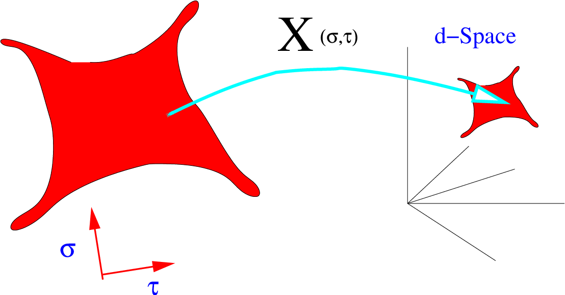
As clear from formula (3), the Veneziano amplitude corresponds to an infinitely growing number of states as a function of the level (). Such a spectrum is reminiscent of the classical oscillatory modes of a string. However, the construction of a theory of strings and the identification of the Veneziano amplitude as a particular string interaction amplitude took some time. In the following we will give the structure of the quantum position operator for a (bosonic) string and sketch the derivation of the Veneziano amplitude as the tree-level string interaction amplitude.
In order to describe the degrees of freedom of a relativistic string, it is useful to introduce the following set of bosonic operators:
| (5) |
where one considers for the target space, see Fig. 2, the -dimensional flat metrics
| (6) |
In (5), the operators describe the momentum and position of the string center of mass, while are the bosonic annihilation and creation operators describing the oscillator modes of the string. Using these definition, one builds the string position operator at the boundary as follows
| (7) |
with
| (8) |
The -dependence is restored, specifying the boundary conditions of the open string, by multiplying each term in (8) by
The calculation of the amplitude is made by integration over the world-sheet variables of an overlap over plane wave operators . Introducing the normal ordered vertex operators
| (9) |
the Veneziano amplitude in terms of string vertex operators reads:
| (10) |
where the external states are
| (11) |
and where denotes the vacuum state. The harmonic oscillators acting on this state build the Hilbert space of string states. The fact that three over the four coordinates can be fixed at will comes from the string symmetries which will be discussed in the next section.
Using the definition (9) together with the relation
| (12) |
one finally finds
| (13) |
which is nothing else han the Veneziano amplitude. An important step towards the construction of string theory was made when the suitable generalization to arbitrary number of legs has been performed. The operator formalism was then found and fully confirmed.
[Exercise 3.1: prove formula (12) from relations (5,8), using the Baker-Hausdorff formula if is scalar]
4. String Symmetries
The symmetries play a crucial role in the properties of string theory. Let us discuss the main features of string symmetries. There exists an exact symmetry group on the string worldsheet. It contains, respectively, dilatation, translation and inversion in the worldsheet variable with generators
respectively. These transformations correspond to the infinitesimal generators (the ) of the Projective (conformal) invariance group (its algebra of generators is given further on, see (18)). It is precisely this invariance with 3 generators, which allows one to arbitrarily fix among values of the worldsheet variables in the expression of the amplitude leaving one interation for the Veneziano amplitude (13).
By extension, one also introduces the generalized conformal transforms for all which however will not form an exact symmetry algebra at the quantum level, as we will discuss now. They will give rise to the famous with a “central extension” or quantum anomaly.
As usual in the formulation of symmetries, a key point is to find an appropriate representation of the algebra in terms of physically meaningful objects, here the annihilation and creation operators describing the string. For this sake one forms the following operators
| (14) |
which possess nice algebraic properties, when acting on the string position operator (7).
Let us first consider the set of operators One can prove that
| (15) |
which demonstrate that they form an adequate representation of the algebra of the projective symmetry group More generally one finds
| (16) |
and thus a representation of the generalized projective transformations on the string position operator and thus on the string states.
Now the symmetry properties will come from the commutation relations between the generators, the Virasoro Algebra. One finds
| (17) |
[Exercise 4.2: prove formula (17), starting with the simpler cases when ]
The formula (17) calls for comments. From the algebra, it is easy to note that, restricting (17) to one finds
| (18) |
which is the algebra of generators of the group (analoguous to and its generators , but with a change of sign in the relation which is related to the non-compactness of the group). Hence this subalgebra indicates the exact symmetry under projective transforms.
For higher one notes the extra contribution which is proportional to the target space dimension The “central charge” ( with the conventional normalization) is a fundamental contribution, showing that the generalized projective group is not an exact symmetry (unless other contributions cancel the central charge due to the dimension, which is precisely the condition for the existence of a consistent string theory). It will in fact be crucial in the striking feature of string theory to imply a constraint on the target space, the space in which it moves!
5. Why 26 (or 10) Dimensions?
Now we have the tools to understand the old puzzle which has jeopardized the initial strong-interactions/strings connection. The question is whether one can construct 4-dimensional string amplitudes in Minkowski space and the answer is in fact “no”. Let us list the problems when facing the construction of 4-d strings in a theoretically consistent way. One finds th following problems
i) Open (resp. closed) strings Gauge (resp. Gravity) at lower energy
ii) Zero-mass asymptotic states: gauge bosons, gravitons
iii) Hadron spectrum not compatible
iv) QCD not obtained
v) Problem of dimensions: The Minkowskian string (resp. superstring) target-space is 26 (resp. 10) dimensional
[Exercise 5.1: Given the (spin 1, Mass 770 MeV) and (spin 2, mass 1270 MeV) mesons which are on the dominant hadronic Reggeon trajectory and the fact that total hadronic cross-sections are constant with energy (up to logarithms) illustrate the third point of the list]
Let us consider the problem of dimensions as a major illustration of the deep implications of quantum consistency and symmetries of string theory based on the Virasoro Algebra.
The problem can be viewed in different ways. Here we shall take the point of view of the construction of an Hilbert space made of positive norm particle states. Let us first remind the well-known construction of the Hilbert space for QED.
If one considers the oscillator construction of the QED Hilbert space one is led to satisfy, choosing the covariant gauge, the condition
where denotes the QED analogue (indeed ancestor) of the creation L-operator . As is known from QED quantification, one may classify the four vector states within three categories, namely
In a similar way for strings, and now for the whole hierarchy of operators , one considers the following (covariant) gauge conditions
| (19) |
which allows a similar generalized classification of states
Now, the key point for the construction of a consistent Hilbert space of string states is that spurious states decouple from the other ones. Building a simple example we shall prove that it implies a necessary condition over the target space dimension. For simplicity, we shall not enter in the proof that this is a sufficient condition for eliminating all spurious states from the spectrum.
Let us consider the following spurious state:
| (20) |
[Exercise 5.2: prove that the state defined by formula (20) is indeed spurious if the states are physical on-shell states]
Then acting on with an appropriate combination of operators, one finds
| (21) |
[Exercise 5.3: prove Equation (21) by inserting the state (20) using the Virasoro algebra relation and classifying the obtained states using (Lecture I: String Theory Strong Interactions)]
The decoupling of spurious states requires that the subspace of spurious states should remain orthogonal from the physical spaces. Hence one gets the condition characteristic of the bosonic string consistency. A similar condition applies to the supersymmetric versions of string theory in Minkowskian space, leading to The decoupling of non-physical states is thus directly a consequence of the Virasoro Algebra and more specifically of its central charge properties.
Lecture II: Gauge/Gravity correspondence
6. An Open-Closed String connection
We have discussed in section 5 the drawbacks of the initial attempts to obtain strong interaction physics from string theory. Indeed, on the string-theoretical point of view, the dimensionality of a Minkowskian target space (26 or 10), the existence of zero mass states and their connection to gauge field theory and gravity, among other features, seemed to invalidate a string description of hadronic interactions. On the field-theoretical point of view, based on the existence of a satisfactory theoretical understanding of quark and gluon interactions at weak coupling in terms of Quantum Chromodynamics, the challenge of a correct description of interactions at long distance relies on the still unsolved problem of computing observables at strong coupling. As we shall see now the Gauge/Gravity duality, a deep “geometrical” property of string amplitudes, and its precise formulation in the case of the so-called AdS/CFT correspondence, seem to overcome at least in principle, the difficulties from both string and field theory sides and opens a new way for the string approach to strong interactions.
Let us first give a quite general argument, giving a qualitative explanation of this new way of approaching the problem. It relies on a connection between open and closed strings which is displayed on Fig. 3. We consider the configuration of two stacks of D-branes in the 10-dimensional target space of a superstring theory. The D-branes are kind of “solitonic” objects which form a consistent background in the string-theoretical framework. In particular, they are the locus of open string endpoints. In Fig. 3 they are understood as stacks of branes which are two sets of copies of the Minkowski space, separated by a distance in a fifth dimension, which will play a special role in the following.
One can geometrically interpret the cylinder shape of the interaction in two equivalent ways: i) It may be seen as the propagation of a closed loop, starting on one brane-stack and reaching the second one; ii) It may be seen alternatively as a one-loop contribution from open-strings since open strings may have end-points on branes. This equivalence, once given a precise formulation in terms of a specific string theory, has quite intringuing and far-reaching consequences.


Let us list some of them:
Gauge/Gravity duality. As we have alluded to in section 5, the massless modes of the string states are gauge fields for the open strings and gravitons for the closed strings. Hence the interaction amplitude depicted in Fig. 3 potentially identifies a tree-level gravitational interaction with a gauge one at one-loop.
Short/Long distance relationship. When one consider a large 5th dimensional distance , the closed string exchange is expected to be described by a classical, weakly coupled, gravitational interaction. By contrast, at small distance, the open string interaction is well-described by the exchange of its zero-mode states, that is the gauge vector fields. This is theoretically justified, since the exchange of open strings with multiple combinations of open-string end-points between stacks of near-by branes, are related at weak string coupling to generic gauge field theories (see Fig. 4).
Weak/Strong coupling relationship. At short distance the gauge coupling is weak (due to asymptotic freedom for ). By contrast, the gravitational interaction is expected to become strong since the stacks of branes are some kind of very massive objets and are expected to generate a strong gravitational field in their neighbourhood. On the other end of the comparison, at long distance the gravity is weak, while the open string interaction is expected to become strongly coupled, and moreover, all the excitations of the open strings which correspond to the massive oscillator modes are expected to contribute.
From that comes the main feature of the Gauge/Gravity duality; It makes a deep connection between weak coupling on one side of the correspondence to the strong coupling regime of the other side. It is thus intrinsically a weak/strong coupling duality.
In the present series of lectures, we are interested in the weak gravity/strong gauge coupling combination (the investigation of the weak gauge strong gravity duality is yet another fascinating challenge). Obtaining valuable new tools of investigation of gauge theories at strong coupling from their gravity duals at weak coupling, and thus accessible to a quantitative approach.
7. The AdS/CFT correspondence

The AdS/CFT correspondence has many interesting both formal and physical facets. Concerning the aspects which are of interest for our problem, it allows one to find relations between gauge field theories at strong coupling and string gravity at weak coupling in the limit of large number of colours (). It can be examined quite precisely in the AdS5/CFT4 case where CFT4 is the 4-dimensional conformal field theory corresponding to the gauge theory with supersymmetries.
[Exercise 6.1: How many gauge bosons are expected in Fig. 4?]
Some existing extensions to other gauge theories with broken conformal symmetry and less or no supersymmetries will be valuable for our approach, since they lead to confining gauge theories which are more similar to QCD. Note that the appropriate string gravity dual of QCD has not yet been identified, and thus we are forced to restrict for the moment our use of AdS/CFT correspondence to generic features of confining theories duals, see a discussion further on in this section.
Let us recall the canonical derivation leading to the AdS5 background see Fig. 5. One starts from the (super)gravity classical solution of a system of -branes in a space of the (type IIB) superstrings. The metrics solution of the (super)Einstein equations read
| (22) |
where the first four coordinates are on the brane and corresponds to the coordinate along the normal to the branes. In formula (22), one writes
| (23) |
where is the so-called ‘t Hooft-Yang-Mills coupling equal to the string coupling and the string tension.

One considers the limiting behaviour considered by Maldacena, where one zooms on the neighbourhood of the branes while in the same time going to the limit of weak string slope The near-by space-time is thus distorted due to the (super) gravitational field of the branes. One goes to the limit where
| (24) |
This, from the second equation of (23) obviously implies
| (25) |
i.e. both a weak coupling limit for the string theory and a strong coupling limit for the dual gauge field theory. By reorganizing the two parts of the metrics one obtains
| (26) |
which corresponds to the AdS5 background structure. In (26) describes a Anti de Sitter11 1 the 5-d version of de Sitter geometrical space, whose 4-d version appears in general relativity, has a plus sign, obeys the equation . geometrical space which is a 5-dimensional hyperboloïd of equation in a 6-dimensional flat Minkowski space is the 5-sphere of metric where is the 5-dimensional solid angle. More detailed analysis shows that the isometry group of the 5-sphere may be considered as the “gravity dual” of the supersymmetries (for completion, the quantum number dual to the number of colours, is the invariant charge carried by a Ramond-Ramond form field in (type IIB) superstrings.
In the case of confining backgrounds, an intrinsic scale breaks conformal invariance and is brought in the dual theory through e.g. a geometrical constraint. For instance, a confining gauge theory is expected to be dual to string theory in an Black Hole (BH) background
| (27) |
where and is the position of the BH horizon. One may use this type of background to study the interplay between the confining nature of gauge theory and its reggeization properties. Actually the qualitative arguments and approximations should be generic for most confining backgrounds. For instance, other geometries for (supersymmetric) confining theories have been discussed in this respect. They have the property that for small , the geometry looks like (in up to logarithmic corrections related to asymptotic freedom) giving a coulombic potential. For large the geometry is effectively flat. In all cases there is a scale, similar to above, which marks a transition between the small and large regimes.
8. Wilson Loops, Minimal Surfaces and Confinement
We will find appropriate in the next section to formulate the scattering amplitudes in terms of Wilson loops, since the Gauge/Gravity “dictionnary” for Wilson loops has been proved to be well suitable for dual properties in general. Let us thus introduce this dictionnary in the following. Let us introduce the general framework within which Wilson loops in the “boundary” gauge field theory are in correspondence with minimal surfaces in the “bulk”.

In a framework suitable for performing the AdS/CFT correspondence, quarks (resp. antiquarks) can be represented22 2 In order to get correct quark degrees of freedom, flavor, a more complete geometrical set-up including branes is used. by colour sources in the fundamental (resp. anti fundamental) reps. of SU(N). In order to illustrate the way how one may formulate in practice the AdS/CFT correspondence in a context similar to QCD, let us consider first the example of the vacuum expectation value (vev) of Wilson loops in a configuration parallel to the time direction of the branes. We consider the large time limit and thus the loops close “near” infinity in the time direction (see Fig. 6). This configuration allows a determination of the potential between colour charges. The rôle of colour charges is played by open string states elongated between a stack of branes on one side and one brane near the boundary of AdS space.
The correspondence can be formulated33 3 For simplicity, an extra singlet term in the left-hand exponent, allowing to cancel divergences, is not written here. as follows
| (28) |
where is the Wilson loop contour near the branes and any surface in -space with as the boundary, see Fig. 6.
In the semi-classical approximation for the right-hand (gravity) side of the relation (28) where the Gauge/Gravity correspondence would give the strong coupling value of the left-hand (gauge) side, the integration over surfaces boils down to
| (29) |
where is the minimal surface whose boundary is the gauge-theory Wilson loop. The factor denoted refers to the fluctuation determinant around the minimal surface, corresponding to the first quantum correction beyond the classical approximation. It gives an interesting calculable semi-classical correction, as we shall see on the amplitude exemple.
In Fig. 6, we have sketched the form of minimal surface solutions for the “confining” case, (see above (27)). For large separation of Wilson lines, the minimal surface is bounded near the horizon and is consequently curved. At smaller separation, the solution becomes again similar to the conformal case, since the horizon cut-off does not play a big rôle.
In gauge theory, the quark-quark potential is known to be obtained from a suitable time-like infinite limit of the rectangular Wilson loop vev. One has
| (30) |
Thanks to the Gauge/Gravity correspondence (28) and the classical approximation (29), one is able to get the strong coupling limit of the interquark potential from the large time limit of the Wilson loop v.e.v.:
where are constants. The potential behaviour obeys the nonconfining Coulomb law for the case and the confining law for the case. An interesting nonanalytic dependence over the square-root coupling appears. Note again that, even in the case of a confining geometry with an horizon at Wilson lines separated by a distance do not give rise to minimal surfaces sensitive to the horizon (see Fig. 3), and thus to classical solutions similar to the non-confining case, which can give interesting indications for small spatial separation.
The important rôle of fluctuation corrections and the way of computing it in some non-trivial cases will be discussed further on.
9. Application: A dual model for Dipole Amplitudes


Now we will come back to our original problem of describing in a consistent way the strong interaction two-body amplitudes which correspond, to the processes depicted in fig.1. There are different approaches to scattering amplitudes using gravity duals, including recently the formulation of gluon amplitudes at strong coupling in the gauge theory with supersymmetries. However, since we are interested in the present lecture in the approach to hadronic scattering amplitudes, we search for both a field-theoretical formulation based on QCD and the determination of the gravity duals of the corresponding amplitudes. Concerning the nature of the dual theory, the gravity dual theory of QCD has not yet been identified. More generally, the problem of deriving a correspondence for a confining theory with asymptotic freedom is not yet achieved. In the following we shall use an approach where only generic features of confining backgrounds allow to determine some properties of the amplitudes. The price we pay is that we will only be able to discuss the high-energy behaviour of the amplitudes, the high-energy regime, which was discussed in section 2 for instance in Eq.(4). Other properties of the amplitudes will not be discussed, and probably are more difficult to derive in the absence of a better determined dual background to QCD. Using the AdS/CFT correspondence, we will find that two-body high-energy amplitudes in gauge field theories can be related to specific configurations of minimal surfaces.
Using the Wilson loop properties, it is now possible to formulate the Gauge/Gravity correspondence for the elastic and inelastic scattering amplitude of massive colorless states in the space of QCD color dipoles. In Fig. 7, one displayed the elastic and inelastic amplitudes of two dipoles in configuration space, corresponding respectively to , and appearing in Lecture I. We will here consider the amplitudes at high energy, i.e. the problem of “Reggeization”. Indeed, at high energy, fast moving colour sources propagate along linear trajectories in coordinate space thanks to the eikonal approximation. This important property of high energy propagation of color sources will be helpful for the evaluation of the amplitudes through Gauge/Gravity duality.
Let us first consider the elastic dipole amplitude, the left diagram of Fig. 7. In the gauge field theory, one may write it in terms of a correlator between two Wilson lines in configuration space, namely
| (31) |
where the Wilson loops corresponding to the two colliding dipoles follow classical straight lines for quark(antiquark) trajectories and close at infinite time, as for the potential. The normalization of the correlator ensures that the amplitude vanishes when the Wilson loops get decorrelated at large distances.
One useful technique is to formulate the duality property in Euclidean space where it takes the form of a well-defined geometrical interpretation in terms of a minimal surface problem. Then the analytic continuation from Euclidean to Minkowski space allows one to find the physical solution.
The Wilson line vev can be expressed as a minimal surface problem with (approximately) two copies (for dipole size ) of a minimal surface whose boundaries are straight lines in a 3-dimensional coordinate space, placed at an impact parameter distance and rotated one with respect to the other by an angle see Fig. 7. then the amplitude will be obtained through the analytic continuation
| (32) |
where is the total rapidity interval.
In flat space, with the same boundary conditions, the minimal surface is the helicoid. One thus realizes that the problem can be formulated as a minimal surface problem whose mathematically well-defined solution is a generalized helicoidal manifold embedded in curved background spaces, such as Euclidean AdS Spaces. Unfortunately, this problem is rather difficult to solve analytically, even in flat space. It is known as the Plateau problem, namely the determination of minimal surfaces for given boundary conditions.
In fact, the definition of the minimal surface geometry in the conditions of a confined metrics (27) appears to be simpler, at least for the leading contribution. Indeed, in the configuration of Wilson lines of Fig. 6 in the context of a confining theory, the AdSBH metrics is characterized by a singularity at which implies a rapid growth in the direction towards the D3 branes, then stopped near the horizon at Thus, to a good approximation, and for a large enough impact parameter (compared to the horizon distance), the main contribution to the minimal area is from the metrics in the bulk near which is nearly flat. Hence, near the relevant minimal area can be drawn on a classical helicoid, whose analytic expression is known. This expression contains a logarithmic singularity in terms of kinematical variables, which turns out to be essential to generate an imaginary part in the action after analytic continuation to Minkowski space.
After analytic continuation, one obtains
| (33) |
which represents a Reggeized elastic amplitude, with a linear Regge trajectory
| (34) |
characterized by a Pomeron intercept and a Regge slope, defined in terms of the gravity dual parameters by where is the string or ‘t Hooft coupling.
Let us now consider the dipole-dipole inelastic amplitude
| (35) |
represented in configuration space on Fig. 7, right. The helicoidal geometry remains valid due to the eikonal approximation for the “spectator quarks”, namely the and Wilson lines while the “exchanged quarks” define a trajectory drawn on the helicoid. This trajectory plays the rôle of a dynamical time-like cut-off which takes part in the minimization procedure. The resulting amplitude reads:
| (36) |
corresponding to a linear Regge trajectory
| (37) |
characterized by a “Reggeon” intercept and a Regge slope Note that the slope is related to the quark potential calculated within the same AdS/CFT framework and, quite interestingly we find , to be compared with the string result at weak coupling
Up to now, we restricted ourselves to a classical approximation based on the evaluation of minimal surfaces solutions for the various Wilson loops involved in the preceeding calculations. It is interesting to note that a further step can be done by evaluating the contribution of quadratic fluctuations of the string worldsheet around the minimal surfaces in the case where these surfaces are embedded in helicoids, as discussed for the confining backgrounds. The semi classical correction comes from the fluctuations near the minimal surface. The main outcome is that this semi classical correction can be computed and is intimately related to the well-known “universal” Lüscher term contribution to the interquark potential.
After some non-trivial steps, the formulae (33,36) get corrected as follows
| (38) |
where is the number of zero modes of the gravity dual theory in the transverse-to-the-branes directions. The result is just equivalent to the known Lüscher term in found in the large-time expansion of the rectangular Wilson loop, except that the number of zero modes can be larger than the usual value (=2) corresponding to flat space.
It is interesting to note that this theoretical feature is in qualitative agreement with the phenomenology of soft scattering. Indeed once we fix the from the phenomenological value of the static potential () we get for the slopes and in good agreement with the phenomenological slopes.
A second feature is the relation between the Pomeron and Reggeon intercepts. At the classical level of our approach these are respectively and Note that this classical contribution matches what is obtained from simple exchanges of two gluons and quark-antiquark pair, respectively, in the channel. The fluctuation (quantum) contributions to the Reggeon and Pomeron are also related by the factor .
Adding both classical and fluctuation contributions gives an estimate which is in qualitative agreement with the observed intercepts. Indeed, when calculating the fluctuations around a minimal surface near the horizon in the BH backgrounds there could be massless bosonic modes. For one gets for the Pomeron and for the Reggeon. This result is in agreement with the observed intercept for the “Pomeron” and somewhat below the intercepts observed for the dominant Reggeon trajectories. The interesting output of the application of AdS/CFT correspondence to high energy amplitudes at strong coupling is to emphasize the relation between Reggeization and confinement, using the description of two-body scattering amplitudes in the dual string theory.
Lecture III: Quark-Gluon Plasma/Black Hole Duality
10. QGP formation and Hydrodynamics

The formation of a QGP (Quark Gluon Plasma) is expected to be realized in high-energy heavy-ion collisons, e.g. at RHIC and soon at the LHC. One of the main tools for the description of such a formation is the relevance of relativistic hydrodynamic equations in some intermediate stage of the collisions, see Fig. 8. The problem of the hydrodynamic description is the somewhat indirect relation with the underlying fundamental theory. Indeed, the experimental observations seem to indicate an almost perfect-fluid behaviour with small shear viscosity, which naturally leads to consider a theory at strong coupling and thus within the yet unknown non-perturbative regime of QCD. Moreover the QGP formation appears to be fast, which may also point towards strong coupling properties. Another key point of the standard description is the approximate boost-invariance of the process in the central rapidity region, that is the well-known Bjorken flow. The goal of the string theoretic approach is to make use of the Gauge/Gravity correspondence as a way to tackle the problem of the hydrodynamic behaviour from the fundamental theory point of view. It allows to draw quantitative relations between a strongly coupled gauge field theory and a weakly coupled string theory
More specifically, the AdS/CFT correspondence between the supersymmetric gauge theory and superstrings in 10 dimensions can be used as a calculational laboratory for this kind of approach, at least as a first stage before a more realistic application to QCD. The unconfined character of the QGP gives some hope that the explicit AdS/CFT example could be useful despite the lack of asymptotic freedom and other aspects specific of QCD.
11. AdS/CFT and Holographic Hydrodynamics
One typical and fascinating aspect of the Gauge/Gravity duality is the property of as we have seen in section 8. It states that the amount of information contained in the boundary gauge theory (on the brane) is the same as the one contained in the bulk string theory. In our problem, we shall make use in a quantitative way of this property by taking advantage of one of the remarkable relations due to the “holographic renormalization”. Using the Fefferman-Graham coordinate system for the metric
One can write
| (39) |
where is the bulk metric in 5 dimensions, the boundary metric in physical (3+1) Minkowski space and the v.e.v. of the physical energy-momentum tensor. The higher coefficients of the expansion over the fifth dimension can be obtained by the Einstein equations in the bulk provided the boundary energy-momentum tensor fulfils the zero-trace and continuity equations. It is important to note that the relation (39) to be valid requires for the boundary energy-momentum tensor, by consistency
which are nothing else than the properties of a physical 4-d with the zero trace condition of a conformal theory, verified by the perfect fluid.
The interesting observation on which we shall elaborate, namely that there is a non-trivial dual relation between a perfect fluid at rest in (3+1) dimensions and a static 5d black hole in the bulk can be proven using holographic renormalization. Indeed, let us consider the perfect fluid with a stress-energy tensor equipped with diagonal elements
where is the energy density and is the pressure density. One can resum the whole holographic expansion (39) and get the following bulk metric in Fefferman-Graham coordinates
| (40) |
[Exercise 12.1: Recover the Energy-Momentum tensor corresponding to the metric (40), by using the expansion (39)]
A change of variable gives
| (41) |
where one recognizes the Black Hole, in fact a black brane, with a static horizon at in the 5th dimension.
In fact there exists a one-to-one correspondence between the thermodynamic properties of the Black Hole () and those of the perfect fluid (), namely its temperature () and entropy ().
It is in this context of a static Black Hole configuration that one can go further than the perfect fluid approximation and derive the viscosity using the Kubo formula. Indeed, the duality properties extend to a relation between the correlators of the energy-momentum tensor in two space-time points at zero frequency and the absorption cross section of a graviton by the static BH in the bulk. One writes
| (42) |
where is the famous entropy-area relation of a Black Hole. From this relation, and putting numbers, it appears that the viscosity is weak, much weaker than the one computed in the weak coupling regime and eventually realizing an absolute viscosity lower bound.
12. QGP and Black Holes: From Statics to Dynamics

The previous results were obtained for static configurations, for a thermalized QGP at rest. In order to take into account, as much as possible, the actual kinematics of a heavy-ion collision, it is required to introduce the proper time expansion of the plasma. On the gravity side, it calls for studying non-equilibrium geometries, eventually of 5d BH configurations, which represent in itself a non-trivial and interesting issue. Dual geometries to the standard “Bjorken flow” where recently constructed. The Bjorken flow is the description of a boost-invariant expansion of the QGP, which is expected to correspond to the physical situation in the central rapidity region of the collision. In this context the questions why the QGP fluid appears to be nearly perfect (small viscosity) and why its thermalization time can be short have been adressed.
Let us consider the equations obeyed by a physical energy-momentum tensor expressed in the coordinate system:
|
|
(43) |
In a boost-invariant framework, one may consider a general family of solutions of proper time dependent, boundary energy-momentum tensors
| (44) |
where the function satisfying the positivity condition
corresponds to an interpolation between different relevant regimes, namely
Perfect fluid
Free streaming
“Full anisotropy”
Using the holographic renormalization to compute the coefficients of the corresponding metrics in the expansion on the fifth dimension and after resummation, it was possible to solve the dual geometry for given at asymptotic proper time It reveals the existence of a scaling property of the solutions in terms of the proper time dependent variable
Analyzing the family of solutions as a function of it appears that the only non-singular solution for invariant scalar quantities (here the square of the Ricci tensor see Fig. 9), is obtained for Indeed, we find in Fefferman-Graham coordinates:
which is similar to the metrics of the static Black Hole (40), but substituting This solution is the only one of the family corresponding to a Black Hole moving away in the fifth dimension. Hence the perfect-fluid case is singled out and the moving BH in the bulk corresponds through duality to the expansion of the QGP taking place in the boundary. Consequently, the BH horizon moves as the temperature as and the entropy stays constant since Note that again the physical thermodynamical variables of the QGP are the same as those one may attribute to the BH in the bulk (with the reservation that thermodynamics of a moving BH may rise non-trivial interpretation problems). Hence one finds a concrete realization of the idea of a duality between the QGP formation and a moving Black Hole.
13. Thermalization and Isotropization
There has been a lot of activity along the lines of the AdS/CFT correspondence and its extensions to various geometric configurations. Dual studies of jet quenching, quark dragging , etc… have been and are still being performed. Sticking to the configurations corresponding to an expanding plasma and going beyond the first order terms in proper time, one has obtained results on the viscosity, confirming the universal value (42), on the relaxation time of the plasma and very recently on the inclusion of flavor degrees of freedom.
Let us finally focus on the thermalization problem, which can be usefully taken up using the Gauge/Gravity duality in the strong coupling hypothesis. the problem is to give an explanation to the strikingly small thermalization time required for the formation of a QGP as can be abstracted from the experimental observations. Analyzing the stability of the expanding plasma configuration, it has been found that performing a small deviation from the BH metric by coupling with a scalar field and analyzing the corresponding quasi-normal modes defining the way how the system relaxes towards its initial state, one finds a numerically small value of the relaxation time in units of the local temperature. Even if a definite value of this relaxation time cannot be inferred at this stage due to scale-invariance, this result was suggestive of a stability of the QGP in the strong coupling regime with respect to perturbations out of equilibrium.
In order to go further, one has to deal with the problem of the QGP evolution at small proper times. The holographic renormalization program has been pursued for the small proper time expansion. Relaxing the selection of the appropriate metric by requiring only the metric tensor to be a real and single valued function of the coordinates everywhere in the bulk, one finds an unique solution corresponding to the “fully anisotropic case”

In the same paper, an evaluation of the range of the isotropization time has been proposed, by extrapolation of realistic estimates abstracted from experiments to the supersymmetric case. The idea is to match the large and small proper time regimes at some value of the proper time This proper time is mathematically defined as the crossing value for the branch-point singularities of both regimes. Physically, it is expected to give an estimate of the proper time range during which which the medium evolves from the full anisotropic regime (small ) to the perfect fluid one (large ).
In order to give an idea of the possible physical implications of this strong coupling scheme, let us shortly reproduce the argument. Implementing the estimated physical value of the energy density at some proper time () one finds
| (45) |
This short isotropization time thus seems a characteristic feature of the strong coupling scenarios. It is clear that more realistic estimates should take into account less idealized dual models, corresponding to QCD, such as the lack of supersymetry and the finite numbers of colors. However, the non confined character of the QGP and the robustness of some predictions (such as the ratio) may give some confidence that this short isotropization time could be a reasonable estimate at strong coupling.
14. Outlook
From the present rapid (and partial) survey of some of the results obtained in the AdS/CFT approach to the formation and expansion of the Quark-Gluon plasma in heavy-ion collisions, it appears that the Gauge Gravity correspondence is a promising way to explore some features of QCD at strong coupling. Indeed some general features of this correspondence, relating at long distances the closed and open string geometries (see Fig. 3) are expected to be valid in principle for various dual schemes and thus, hopefully, QCD.
In practice, the quantitative dual schemes have been more precisely elaborated for the specific AdS/CFT case, the gauge theory with supersymmetries. Among the results, it gives a calculable link between the hydrodynamic quasi-perfect fluid behaviour on the “gauge theory side” with a BH geometry in the higher dimensional “gravity side” in an AdS background. This relation can be extended from the static case to a dynamical regime reflecting (within the AdS/CFT framework) the relativistic expansion of the corresponding quark-gluon plasma. This, and many other applications, some of them using more complex geometries, less supersymmetric backgrounds and examining other observables, gives hope for the fruitful possibilities of the Gauge/Gravity approach to the QGP formation.
As an outlook, it is worth mentionning some of the possible new directions of study one is led to consider. Starting with the more technical ones, it is known that the Bjorken flow is not exactly verified in heavy-ion collisions, since the observed distribution of particles is nearly gaussian in rapidity and thus not reflecting exactly the boost-invariance of the Bjorken flow. It would be interesting to investigate dual properties for non-boost invariant flows, such as the Landau flow. On a more general ground, the whole approach still concerns only the hydrodynamical stage of the QGP expansion. It would be important to attack both the initial (partonic) and final (hadronic) stages of the reaction in the same framework and thus the problem of phase transitions during the collision. Finally, one would like to have more realistic dual frameworks including a finite number of colors, flavor degrees of freedom and no (or broken) supersymmetry.
Acknowledgements
I would like to thank Romuald Janik (Jagelonian University, Cracow) for a fruitful and inspiring long-term collaboration between a string theorist and a particle phenomenologist. Emmanouil Saridakis, Alessandro Papa and Christophe Royon are thanked for helping to correct the manuscript.
Note on Lecture I
The lecture I is based on an introduction to string theory the strong interaction peoblems, and thus follows more or less the historical development. Starting with Veneziano’s initial paper, we were largely inspired by the two next references of the list. The first one is a book which has the merit to give the whole derivation (with detailed calculations) of the introduction to string theory the strong interaction paradigm. The second one is very helpful in understanding the story of the discovery of string theory and containing an abundant and documented list of references placed in their historical perspective (as captivating as a detective novel). Moreover a large part of the derivation that I used is here given with useful details.
Nowadays, string theory has developped as an autonomous theory, and many deep properties and its modern ways of introduction are far from the initial problematics. For primary instance the intimate connection of string theory to 2-dimensional conformal field theory do (and did) not appear immediately from the construction of the Hilbert space through scattering amplitudes as sketched in lecture I. Hence it is strongly advised for the students who would like to learn string theory to refer to modern textbooks. My colleagues string theorists would, among others, recommend the two last references of the list, and find there the appropriate references. I make my apologizes to all contributors to string theory for not quoting them directly in the lecture for sake of simplicity (and possible misunderstanding from my part).
Note on Lecture II
The lecture II is based on an elementary introduction to the AdS/CFT correspondence. In a considerably shortened and subjective selection on the enormous literature on the subject the three first references are the original ones. The fourth one is a now rather old but still precious and readable review on the subject. In the general argumentation about gauge/gravity duality, we were inspired by the nice introduction of Ref.[10].
In introducing some concepts useful in the approach to the formulation of hadronic scattering amplitudes at strong coupling, we used mainly the duality vocabulary related to Wilson loops. We quote some relevant original references, and for the rest refer to the review [7].
The specific approach to dipole scattering amplitudes described in the text comes from a collaboration with Romuald Janik, as quoted in the references.
Note on Lecture III
The lecture III is based on a series of papers using the AdS/CFT correspondence as a laboratory for the flow of a strongly coupled quark-gluon plasma. It relies both on the phenomenological validity of the relativistic hydrodynamic approach to the real experiments and its surprisingly good relevance for the Gauge/Gravity correspondence.
The first set of references recall some basic facts about 1+1 relativistic hydrodynamic equations applied to particle collisions concerning the canonical Bjorken and Landau flows and including a recent interpolating family of exact solutions.
The second set of references begins with holographic renormalization, which is a basic tool used in holographic reconstruction followed by original references on the emergence and calculations of the dual Black Hole geometry of a static plasma. In a third set are given some the original references corresponding to the expanding plasma geometry and its evolving black hole dual.
We display at the end a very limited number of references concerning other interesting aspects of the quark gluon plasma problems treated from the point of view of the AdS/CFT correspondence and which were not addressed in this lecture. However the general set-up described here may help for the understanding of the various approaches.
References
- [1] G. Veneziano, “Construction of a crossing - symmetric, Regge behaved amplitude for linearly rising trajectories,” Nuovo Cim. A 57 (1968) 190.
- [2] P. H. Frampton, “Dual Resonance Models And Superstrings,” Singapore, Singapore: World Scientific ( 1986) 539p.
- [3]
P. Di Vecchia,
“The birth of string theory,”
arXiv:0704.0101 [hep-th];
P. Di Vecchia and A. Schwimmer, “The beginning of string theory: a historical sketch,” arXiv:0708.3940 [physics.hist-ph]. Contribution to the volume ‘String theory and fundamental interactions’, dedicated to Gabriele Veneziano on his 65th birthday. - [4] D. Lust and S. Theisen, “Lectures on string theory,” Lect. Notes Phys. , Springer-Verlag 346 (1989) 1.
- [5]
J. Polchinski,
“String theory. Vol. 1: An introduction to the bosonic string,”
Cambridge, UK: Univ. Pr. (1998) 402 p;
“String theory. Vol. 2: Superstring theory and beyond,” Cambridge, UK: Univ. Pr. (1998) 531 p. ———AdS/CFT————– - [6] J. M. Maldacena, “The large N limit of superconformal field theories and supergravity,” Adv. Theor. Math. Phys. 2, 231 (1998) [Int. J. Theor. Phys. 38, 1113 (1999)].
- [7] S. S. Gubser, I. R. Klebanov and A. M. Polyakov, “Gauge theory correlators from non-critical string theory,” Phys. Lett. B 428, 105 (1998).
- [8]
E. Witten,
“Anti-de Sitter space and holography,”
Adv. Theor. Math. Phys. 2, 253 (1998);
“Anti-de Sitter space, thermal phase transition, and confinement in gauge theories,” Adv. Theor. Math. Phys. 2, 505 (1998). - [9] O. Aharony, S. S. Gubser, J. M. Maldacena, H. Ooguri and Y. Oz, “Large N field theories, string theory and gravity,” Phys. Rept. 323, 183 (2000).
- [10] V. Schomerus, “Strings for Quantumchromodynamics,” Int. J. Mod. Phys. A 22, 5561 (2007). ———Wilson Loops and AdS/CFT————–
- [11] J. M. Maldacena, “Wilson loops in large N field theories,” Phys. Rev. Lett. 80, 4859 (1998).
- [12] S. J. Rey and J. T. Yee, “Macroscopic strings as heavy quarks in large N gauge theory and anti-de Sitter supergravity,” Eur. Phys. J. C 22, 379 (2001).
- [13] J. Sonnenschein and A. Loewy, “On the supergravity evaluation of Wilson loop correlators in confining theories,” JHEP 0001, 042 (2000). ———Dual model for dipole amplitudes————–
- [14]
R. A. Janik and R. Peschanski,
“High energy scattering and the AdS/CFT correspondence,”
Nucl. Phys. B 565, 193 (2000);
“Minimal surfaces and Reggeization in the AdS/CFT correspondence ,” Nucl. Phys. B 586, 163 (2000);
Reggeon exchange from AdS/CFT,” “Nucl. Phys. B 625, 279 (2002). ———-Relativistic Hydrodynamics————— - [15] J. D. Bjorken, “Highly Relativistic Nucleus-Nucleus Collisions: The Central Rapidity Region,” Phys. Rev. D 27, 140 (1983).
- [16] L. D. Landau, “On the multiparticle production in high-energy collisions,” Izv. Akad. Nauk Ser. Fiz. 17, 51 (1953).
- [17] A. Bialas, R. A. Janik and R. Peschanski, “ Unified description of Bjorken and Landau 1+1 hydrodynamics,” Phys. Rev. C 76, 054901 (2007). ———-AdS/CFT and Hydrodynamics—————
- [18] K. Skenderis, “Lecture notes on holographic renormalization,” Class. Quant. Grav. 19, 5849 (2002).
- [19]
R. C. Myers,
“ Stress tensors and Casimir energies in the AdS/CFT correspondence,”
Phys. Rev. D 60, 046002 (1999);
V. Balasubramanian, J. de Boer and D. Minic, “ Mass, entropy and holography in asymptotically de Sitter spaces,” Phys. Rev. D 65, 123508 (2002). - [20] G. Policastro, D. T. Son and A. O. Starinets, “The shear viscosity of strongly coupled N = 4 supersymmetric Yang-Mills plasma,” Phys. Rev. Lett. 87, 081601 (2001).
- [21] D. T. Son and A. O. Starinets, “ Viscosity, Black Holes, and Quantum Field Theory,” Ann. Rev. Nucl. Part. Sci. 57, 95 (2007). ———-AdS/CFT for an Expanding Plasma—————
- [22]
H. Nastase,
“ The RHIC fireball as a dual black hole,”
E. Shuryak, S. J. Sin and I. Zahed, “A gravity dual of RHIC collisions,” J. Korean Phys. Soc. 50, 384 (2007). - [23]
R. A. Janik and R. B. Peschanski,
“Asymptotic perfect fluid dynamics as a consequence of AdS/CFT,”
Phys. Rev. D 73, 045013 (2006);
“Gauge / gravity duality and thermalization of a boost-invariant perfect fluid,” Phys. Rev. D 74, 046007 (2006). - [24]
S. Nakamura and S. J. Sin,
“ A holographic dual of hydrodynamics
JHEP 0609, 020 (2006)
;
R. A. Janik, “Viscous plasma evolution from gravity using AdS/CFT,” Phys. Rev. Lett. 98, 022302 (2007) ;
M. P. Heller and R. A. Janik, “Viscous hydrodynamics relaxation time from AdS/CFT,” Phys. Rev. D 76, 025027 (2007);
J. Große, R. A. Janik and P. Surowka, “Flavors in an expanding plasma,” Phys. Rev. D 77, 066010 (2008). - [25] Y. V. Kovchegov and A. Taliotis, “ Early time dynamics in heavy ion collisions from AdS/CFT correspondence,” Phys. Rev. C 76, 014905 (2007). ———-Other AdS/CFT studies—————
- [26] H. Liu, K. Rajagopal and U. A. Wiedemann, “Calculating the jet quenching parameter from AdS/CFT,” Phys. Rev. Lett. 97, 182301 (2006).
- [27] S. S. Gubser, “Drag force in AdS/CFT,” Phys. Rev. D 74, 126005 (2006).
- [28] C. P. Herzog, A. Karch, P. Kovtun, C. Kozcaz and L. G. Yaffe, “ Energy loss of a heavy quark moving through N = 4 supersymmetric Yang-Mills plasma,” JHEP 0607, 013 (2006).