跳到论文正文
W Papers独立论文阅读器 arXiv:0804.3035 论文正文 计算阅读时间 · 0%
引用这篇论文根据当前论文元数据生成,正式投稿前建议核对。


License: arXiv.org perpetual non-exclusive license
arXiv:0804.3035v2 [math-ph] 04 Nov 2008

Anisotropic growth of random
surfaces in 2+12+1 dimensions

Alexei Borodin ††thanks: California Institute of Technology and Institute for Information Transmission Problems, Moscow, e-mail: borodin@caltech.edu    Patrik L. Ferrari ††thanks: Weierstrass Institute of Applied Analysis and Stochastics (WIAS), Berlin. Now at the Institute for Applied Mathematics, Bonn University.
e-mail: ferrari@wiener.iam.uni-bonn.de
November 4, 2008
Abstract

We construct a family of stochastic growth models in 2+12+1 dimensions, that belong to the anisotropic KPZ class. Appropriate projections of these models yield 1+11+1 dimensional growth models in the KPZ class and random tiling models. We show that correlation functions associated to our models have determinantal structure, and we study large time asymptotics for one of the models.

The main asymptotic results are: (1) The growing surface has a limit shape that consists of facets interpolated by a curved piece. (2) The one-point fluctuations of the height function in the curved part are asymptotically normal with variance of order ln⁡(t)\ln(t) for time t≫1t\gg 1. (3) There is a map of the (2+1)(2+1)-dimensional space-time to the upper half-plane ℍ\mathbb{H} such that on space-like submanifolds the multi-point fluctuations of the height function are asymptotically equal to those of the pullback of the Gaussian free (massless) field on ℍ\mathbb{H}.

1 Introduction

In recent years there has been a lot of progress in understanding large time fluctuations of driven interacting particle systems on the one-dimensional lattice, see e.g. [4, 2, 1, 47, 30, 29, 38, 45, 25, 48, 46, 8, 9, 11, 7, 10]. Evolution of such systems is commonly interpreted as random growth of a one-dimensional interface, and if one views the time as an extra variable, the evolution produces a random surface (see e.g. Figure 4.5 in [43] for a nice illustration). In a different direction, substantial progress have also been achieved in studying the asymptotics of random surfaces arising from dimers on planar bipartite graphs, see the review [32] and references therein.

Although random surfaces of these two kinds were shown to share certain asymptotic properties (also common to random matrix models), no direct connection between them was known. One goal of this paper is to establish such a connection.

We construct a class of two-dimensional random growth models (that is, the principal object is a randomly growing surface, embedded in the four-dimensional space-time). In two different projections these models yield random surfaces of the two kinds mentioned above (one reduces the spatial dimension by one, the second projection is fixing time). We partially compute the correlation functions of an associated (three-dimensional) random point process and show that they have determinantal form that is typical for determinantal point processes.

For one specific growth model we compute the correlation kernel explicitly, and use it to establish Gaussian fluctuations of the growing random surface. We then determine the covariance structure.

Let us describe our results in more detail.

1.1 A two-dimensional growth model

Consider a continuous time Markov chain on the state space of interlacing variables

𝒮(n)={{xkm}k=1,…,mm=1,…,n⊂ℤn⁡(n+1)2|xk−1m<xk−1m−1≤xkm},n=1,2,….{\cal S}^{(n)}=\Big\{\{x_{k}^{m}\}_{\begin{subarray}{ll}k=1,\dots,m\\ m=1,\dots,n\end{subarray}}\subset\mathbb{Z}^{\frac{n(n+1)}{2}}\,|\,x^{m}_{k-1}<x_{k-1}^{m-1}\leq x_{k}^{m}\Big\},\quad n=1,2,\ldots. (1.1)

xkmx_{k}^{m} can be interpreted as the position of particle with label (k,m)(k,m), but we will also refer to a given particle as xkmx_{k}^{m}. As initial condition, we consider the fully-packed one, namely at time moment t=0t=0 we have xkm​(0)=k−m−1x_{k}^{m}(0)=k-m-1 for all k,mk,m, see Figure 1.1.

Refer to caption
Figure 1.1: Illustration of the initial conditions for the particles system and the corresponding lozenge tilings. In the height function picture, the white circle has coordinates (x,n,h)=(−1/2,0,0)(x,n,h)=(-1/2,0,0).

The particles evolve according to the following dynamics. Each of the particles xkmx_{k}^{m} has an independent exponential clock of rate one, and when the xkmx_{k}^{m}-clock rings the particle attempts to jump to the right by one. If at that moment xkm=xkm−1−1x_{k}^{m}=x_{k}^{m-1}-1 then the jump is blocked. If that is not the case, we find the largest c≥1c\geq 1 such that xkm=xk+1m+1=⋯=xk+c−1m+c−1x_{k}^{m}=x_{k+1}^{m+1}=\dots=x_{k+c-1}^{m+c-1}, and all cc particles in this string jump to the right by one. For any t≥0t\geq 0 denote by ℳ(n)​(t){\cal M}^{(n)}(t) the resulting measure on 𝒮(n){\cal S}^{(n)} at time moment tt.

Informally speaking, the particles with smaller upper indices are heavier than those with larger upper indices, so that the heavier particles block and push the lighter ones in order for the interlacing conditions to be preserved. This anisotropy is essential, see more details in Section 1.4.

Let us illustrate the dynamics using Figure 1.2, which shows a possible configuration of particles obtained from our initial condition. If in this state of the system the x13x_{1}^{3}-clock rings, then particle x13x_{1}^{3} does not move, because it is blocked by particle x12x_{1}^{2}. If it is the x22x_{2}^{2}-clock that rings, then particle x22x_{2}^{2} moves to the right by one unit, but to keep the interlacing property satisfied, also particles x33x_{3}^{3} and x44x_{4}^{4} move by one unit at the same time. This aspect of the dynamics is called “pushing”.
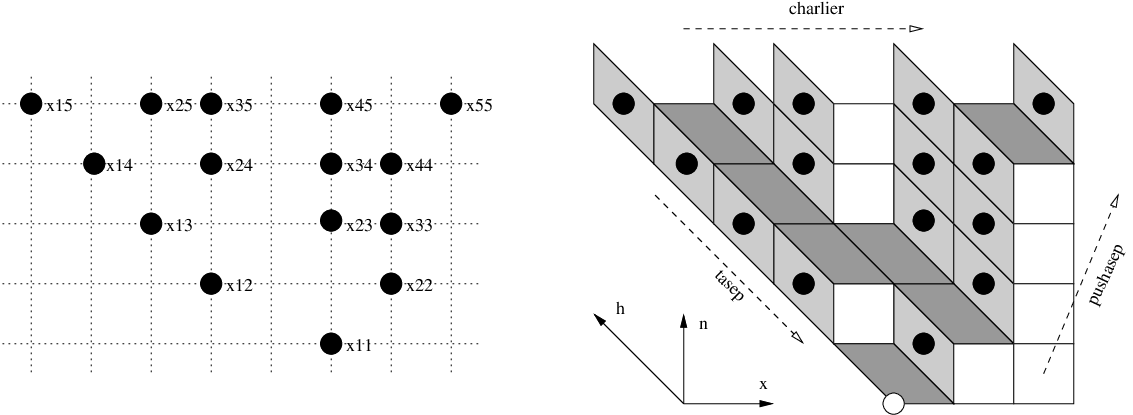
Refer to caption
Figure 1.2: From particle configurations (left) to 3d visualization via lozenge tilings (right). The corner with the white circle has coordinates (x,n,h)=(−1/2,0,0)(x,n,h)=(-1/2,0,0).

Observe that 𝒮(n1)⊂𝒮(n2){\cal S}^{(n_{1})}\subset{\cal S}^{(n_{2})} for n1≤n2n_{1}\leq n_{2}, and the definition of the evolution implies that ℳ(n1)​(t){\cal M}^{(n_{1})}(t) is a marginal of ℳ(n2)​(t){\cal M}^{(n_{2})}(t) for any t≥0t\geq 0. Thus, we can think of ℳ(n){\cal M}^{(n)}’s as marginals of the measure ℳ=lim⟵ℳ(n){\cal M}=\lim\limits_{\longleftarrow}{\cal M}^{(n)} on 𝒮=lim⟵𝒮(n){\cal S}=\lim\limits_{\longleftarrow}{\cal S}^{(n)}. In other words, ℳ⁡(t){\cal M}(t) are measures on the space 𝒮{\cal S} of infinite point configurations {xkm}k=1,…,m,m≥1{\{x_{k}^{m}\}}_{k=1,\dots,m,\,m\geq 1}.

Before stating the main results, it is interesting to notice that the Markov chain has different interpretations. Also, some projections of the Markov chain to subsets of 𝒮(n){\cal S}^{(n)} are still Markov chains.

  1. 1.

    The evolution of x11x_{1}^{1} is the one-dimensional Poisson process of rate one.

  2. 2.

    The row {x1m}m≥1\{x_{1}^{m}\}_{m\geq 1} evolves as a Markov chain on ℤ\mathbb{Z} known as the Totally Asymmetric Simple Exclusion Process (TASEP), and the initial condition x1m​(0)=−mx_{1}^{m}(0)=-m is commonly referred to as step initial condition. In this case, particle x1kx_{1}^{k} jumps to its right with unit rate, provided the arrival site is empty (exclusion constraint).

  3. 3.

    The row {xmm}m≥1\{x^{m}_{m}\}_{m\geq 1} also evolves as a Markov chain on ℤ\mathbb{Z} that is sometimes called “long range TASEP”; it was also called PushASEP in [7]. It is convenient to view {xmm+m}m≥1\{x_{m}^{m}+m\}_{m\geq 1} as particle locations in ℤ\mathbb{Z}. Then, when the xkkx_{k}^{k}-clock rings, the particle xkk+kx_{k}^{k}+k jumps to its right and pushes by one unit the (maybe empty) block of particles sitting next to it. If one disregards the particle labeling, one can think of particles as independently jumping to the next free site on their right with unit rate.

  4. 4.

    For our initial condition, the evolution of each row {xkm}k=1,…,m\{x_{k}^{m}\}_{k=1,\dots,m}, m=1,2,…m=1,2,\dots, is also a Markov chain. It was called Charlier process in [37] because of its relation to the classical orthogonal Charlier polynomials. It can be defined as Doob hh-transform for mm independent rate one Poisson processes with the harmonic function hh equal to the Vandermonde determinant.

  5. 5.

    Infinite point configurations {xkm}∈𝒮\{x_{k}^{m}\}\in{\cal S} can be viewed as Gelfand-Tsetlin schemes. Then ℳ⁡(t){\cal M}(t) is the “Fourier transform” of a suitable irreducible character of the infinite-dimensional unitary group U⁡(∞)U(\infty), see [13]. Interestingly enough, increasing tt corresponds to a deterministic flow on the space of irreducible characters of U⁡(∞)U(\infty).

  6. 6.

    Elements of 𝒮\cal S can also be viewed as lozenge tiling of a sector in the plane. To see that one surrounds each particle location by a rhombus of one type and draws edges through locations where there are no particles, see Figure 1.2. Our initial condition corresponds to a perfectly regular tiling, see Figure 1.1.

  7. 7.

    The random tiling defined by ℳ⁡(t){\cal M}(t) is the limit of the uniformly distributed lozenge tilings of hexagons with side lengths (a,b,c)(a,b,c), when a,b,c→∞a,b,c\to\infty so that a​b/c→tab/c\to t, and we observe the hexagon tiling at finite distances from the corner between sides of lengths aa and bb.

  8. 8.

    Finally, Figure 1.2 has a clear three-dimensional connotation. Given the random configuration {xkn​(t)}∈𝒮\{x_{k}^{n}(t)\}\in{\cal S} at time moment tt, define the random height function

    h:(ℤ+12)×ℤ>0×ℝ≥0→ℤ≥0,\displaystyle h:(\mathbb{Z}+\tfrac{1}{2})\times\mathbb{Z}_{>0}\times\mathbb{R}_{\geq 0}\to\mathbb{Z}_{\geq 0}, (1.2)
    h⁡(x,n,t)=#⁡{k∈{1,…,n}|xkn​(t)>x}.\displaystyle h(x,n,t)=\#\{k\in\{1,\dots,n\}\,|\,x_{k}^{n}(t)>x\}.

    In terms of the tiling on Figure 1.2, the height function is defined at the vertices of rhombi, and it counts the number of particles to the right from a given vertex. (This definition differs by a simple linear function of (x,n)(x,n) from the standard definition of the height function for lozenge tilings, see e.g. [33, 32].) The initial condition corresponds to starting with perfectly flat facets.

Thus, our Markov chain can be viewed as a random growth model of the surface given by the height function. In terms of the step surface of Figure 1.2, the evolution consists of removing all columns of (x,n,h)(x,n,h)-dimensions (1,∗,1)(1,*,1) that could be removed, independently with exponential waiting times of rate one. For example, if x22x_{2}^{2} jumps to its right, then three consecutive cubes (associated to x22,x33,x44x_{2}^{2},x_{3}^{3},x_{4}^{4}) are removed. Clearly, in this dynamics the directions xx and nn do not play symmetric roles. Indeed, this model belongs to the 2+12+1 anisotropic KPZ class of stochastic growth models, see Section 1.4.

1.2 Determinantal formula, limit shape and one-point fluctuations

The first result about the Markov chain ℳ⁡(t){\cal M}(t) that we prove is the (partial) determinantal structure of the correlation functions. Introduce the notation

(n1,t1)≺(n2,t2)iffn1≤n2,t1≥t2, and ​(n1,t1)≠(n2,t2).(n_{1},t_{1})\prec(n_{2},t_{2})\quad\text{iff}\quad n_{1}\leq n_{2},t_{1}\geq t_{2},\text{ and }(n_{1},t_{1})\neq(n_{2},t_{2}). (1.3)
Theorem 1.1.

For any N=1,2,…N=1,2,\dots, pick NN triples

ϰj=(xj,nj,tj)∈ℤ×ℤ>0×ℝ≥0\varkappa_{j}=(x_{j},n_{j},t_{j})\in\mathbb{Z}\times\mathbb{Z}_{>0}\times\mathbb{R}_{\geq 0}

such that

t1≤t2≤⋯≤tN,n1≥n2≥⋯≥nN.t_{1}\leq t_{2}\leq\dots\leq t_{N},\qquad n_{1}\geq n_{2}\geq\dots\geq n_{N}. (1.4)

Then

ℙ{For each j=1,…,N there exists a kj,1≤kj≤nj such that xnjkj(tj)=xj}=det[𝒦(ϰi,ϰj)]i,j=1N,\mathbbm{P}\{\textrm{For each }j=1,\dots,N\textrm{ there exists a }k_{j},\\ 1\leq k_{j}\leq n_{j}\textrm{ such that }x^{n_{j}}_{k_{j}}(t_{j})=x_{j}\}=\det{[{\cal K}(\varkappa_{i},\varkappa_{j})]}_{i,j=1}^{N}, (1.5)

where

𝒦(x1,n1,t1;x2,n2,t2)=−12​π​i∮Γ0d​wwx2−x1+1e(t1−t2)/w(1−w)n2−n1 1[(n1,t1)≺(n2,t2)]+1(2​π​i)2∮Γ0dw∮Γ1dzet1/wet2/z(1−w)n1(1−z)n2wx1zx2+11w−z,{\cal K}(x_{1},n_{1},t_{1};x_{2},n_{2},t_{2})=-\frac{1}{2\pi{\rm i}}\oint_{\Gamma_{0}}\frac{\mathrm{d}w}{w^{x_{2}-x_{1}+1}}\,\frac{e^{(t_{1}-t_{2})/w}}{(1-w)^{n_{2}-n_{1}}}\,\mathbbm{1}_{[(n_{1},t_{1})\prec(n_{2},t_{2})]}\\ +\frac{1}{(2\pi i)^{2}}\oint_{\Gamma_{0}}\mathrm{d}w\oint_{\Gamma_{1}}\mathrm{d}z\frac{e^{t_{1}/w}}{e^{t_{2}/z}}\frac{(1-w)^{n_{1}}}{(1-z)^{n_{2}}}\frac{w^{x_{1}}}{z^{x_{2}+1}}\,\frac{1}{w-z}, (1.6)

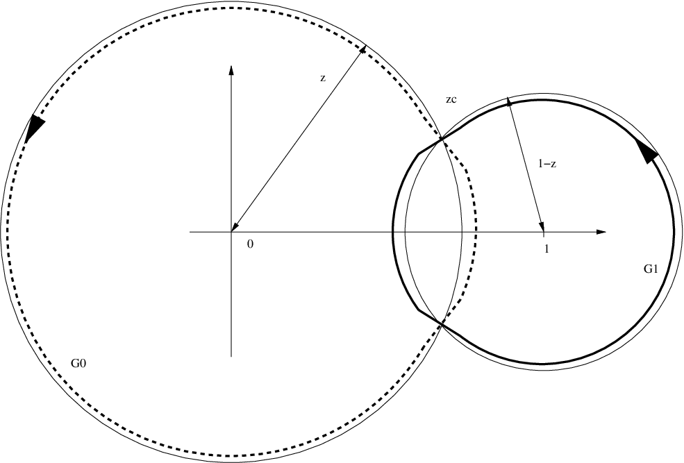
the contours Γ0\Gamma_{0}, Γ1\Gamma_{1} are simple positively oriented closed paths that include the poles 00 and 11, respectively, and no other poles (hence, they are disjoint).

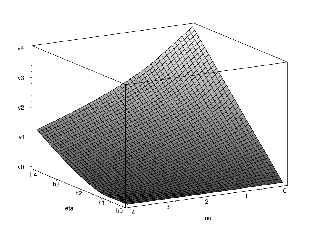
This result is proved at the end of Section 2.8. The above kernel has in fact already appeared in [7] in connection with PushASEP. The determinantal structure makes it possible to study the asymptotics. On a macroscopic scale (large time limit and hydrodynamic scaling) the model has a limit shape, which we now describe, see Figure 1.3. Since we look at heights at different times, we cannot use time as a large parameter. Instead, we introduce a large parameter LL and consider space and time coordinates that are comparable to LL. The limit shape consists of three facets interpolated by a curved piece. To describe it, consider the set

𝒟={(ν,η,τ)∈ℝ>03|(η−τ)2<ν<(η+τ)2}.{\cal D}=\{(\nu,\eta,\tau)\in\mathbb{R}^{3}_{>0}\,|\,(\sqrt{\eta}-\sqrt{\tau})^{2}<\nu<(\sqrt{\eta}+\sqrt{\tau})^{2}\}. (1.7)

It is exactly the set of triples (ν,η,τ)∈ℝ>03(\nu,\eta,\tau)\in\mathbb{R}^{3}_{>0} for which there exists a nondegenerate triangle with side lengths (ν,η,τ)(\sqrt{\nu},\sqrt{\eta},\sqrt{\tau}). Denote by (πν,πη,πτ)(\pi_{\nu},\pi_{\eta},\pi_{\tau}) the angles of this triangle that are opposite to the corresponding sides (see Figure 3.1 too).

Our second result concerns the limit shape and the Gaussian fluctuations in the curved region, living on a ln⁡L\sqrt{\ln{L}} scale.

Theorem 1.2.

For any (ν,η,τ)∈𝒟(\nu,\eta,\tau)\in{\cal D} we have the moment convergence of random variables

limL→∞h⁡([(ν−η)​L]+12,[η​L],τ​L)−𝔼​h​([(ν−η)​L]+12,[η​L],τ​L)κ​ln⁡L=ξ∼𝒩⁡(0,1),\lim_{L\to\infty}\frac{h([\bigl(\nu-\eta)L]+\tfrac{1}{2},[\eta L],\tau L\bigr)-\mathbbm{E}h([\bigl(\nu-\eta)L]+\tfrac{1}{2},[\eta L],\tau L\bigr)}{\sqrt{\kappa\ln{L}}}=\xi\sim{\cal N}(0,1), (1.8)

with κ=(2​π2)−1\kappa=(2\pi^{2})^{-1}.

We also give an explicit formula for the limit shape:

limL→∞𝔼​h​([(ν−η)​L]+12,[η​L],τ​L)L=:h​(ν,η,τ)=1π​(−ν​πη+η⁡(π−πν)+τ​sinπνsinπηsin⁡πτ).\lim_{L\to\infty}\frac{\mathbbm{E}h([\bigl(\nu-\eta)L]+\tfrac{1}{2},[\eta L],\tau L\bigr)}{L}=:\textit{{h}}(\nu,\eta,\tau)\\ =\frac{1}{\pi}\left(-\nu\pi_{\eta}+\eta(\pi-\pi_{\nu})+\tau\,\frac{\sin\pi_{\nu}\sin\pi_{\eta}}{\sin\pi_{\tau}}\right). (1.9)

Theorem 1.2 describes the limit shape h of our growing surface, and the domain 𝒟\cal D describes the points where this limit shape is curved. The logarithmic fluctuations is essentially a consequence of the local asymptotic behavior being governed by the discrete sine kernel (this local behavior occurs also in tiling models [31, 24, 42]). Using the connection with the Charlier ensembles, see above, the formula (1.9) for the limit shape can be read off the formulas of [5].

Using Theorem 1.1 it is not hard to verify (see Proposition 3.2 below) that near every point of the limit shape in the curved region, at any fixed time moment the random lozenge tiling approaches the unique translation invariant measure Mπν,πη,πτM_{\pi_{\nu},\pi_{\eta},\pi_{\tau}} on lozenge tilings of the plane with prescribed slope (see [35, 32, 16] and references therein for discussions of these measures). The slope is exactly the slope of the tangent plane to the limit shape, given by

∂h∂ν=−πηπ,∂h∂η=1−πνπ.\frac{\partial\textit{{h}}}{\partial\nu}=-\frac{\pi_{\eta}}{\pi},\qquad\frac{\partial\textit{{h}}}{\partial\eta}=1-\frac{\pi_{\nu}}{\pi}. (1.10)

This implies in particular, that (πν/π,πη/π,πτ/π)(\pi_{\nu}/\pi,\pi_{\eta}/\pi,\pi_{\tau}/\pi) are the asymptotic proportions of lozenges of three different types in the neighborhood of the point of the limit shape. One also computes the growth velocity (see (1.12) for the definition of Ω\Omega)

∂h∂τ=1π​sinπνsinπηsin⁡πτ=Im⁡(Ω⁡(ν,η,τ))π.\frac{\partial\textit{{h}}}{\partial\tau}=\frac{1}{\pi}\frac{\sin\pi_{\nu}\sin\pi_{\eta}}{\sin\pi_{\tau}}=\frac{\mathrm{Im}(\Omega(\nu,\eta,\tau))}{\pi}. (1.11)

Since the right-hand side depends only on the slope of the tangent plane, this suggest that it should be possible to extend the definition of our surface evolution to the random surfaces distributed according to measures Mπν,πη,πτM_{\pi_{\nu},\pi_{\eta},\pi_{\tau}}; these measures have to remain invariant under evolution, and the speed of the height growth should be given by the right-hand side of (1.11). This is an interesting open problem that we do not address in this paper.

1.3 Complex structure and multipoint fluctuations

To describe the correlations of the interface, we first need to introduce a complex structure. Set ℍ={z∈ℂ|Im⁡(z)>0}\mathbb{H}=\{z\in\mathbb{C}\,|\,\mathrm{Im}(z)>0\} and define the map Ω:𝒟→ℍ\Omega:{\cal D}\to\mathbb{H} by

|Ω⁡(ν,η,τ)|=η/τ,|1−Ω⁡(ν,η,τ)|=ν/τ.|\Omega(\nu,\eta,\tau)|=\sqrt{\eta/\tau},\quad|1-\Omega(\nu,\eta,\tau)|=\sqrt{\nu/\tau}. (1.12)

Observe that arg⁡Ω=πν\arg\Omega=\pi_{\nu} and arg⁡(1−Ω)=−πη\arg(1-\Omega)=-\pi_{\eta}. The preimage of any Ω∈ℍ\Omega\in\mathbb{H} is a ray in 𝒟\cal D that consists of triples (ν,η,τ)(\nu,\eta,\tau) with constant ratios (ν:η:τ)(\nu:\eta:\tau). Denote this ray by RΩR_{\Omega}. One sees that RΩR_{\Omega}’s are also the level sets of the slope of the tangent plane to the limit shape. Since h​(α​ν,α​η,α​τ)=α​h​(ν,η,τ)\textit{{h}}(\alpha\nu,\alpha\eta,\alpha\tau)=\alpha\textit{{h}}(\nu,\eta,\tau) for any α>0\alpha>0, the height function grows linearly in time along each RΩR_{\Omega}. Note also that the map Ω\Omega satisfies

(1−Ω)​∂Ω∂ν=Ω​∂Ω∂η=−∂Ω∂τ,(1-\Omega)\frac{\partial\Omega}{\partial\nu}=\Omega\frac{\partial\Omega}{\partial\eta}=-\frac{\partial\Omega}{\partial\tau}, (1.13)

and the first of these relations is the complex Burgers equation, cf. [34].

From Theorem 1.2 one might think that to get non-trivial correlations we need to consider (h−𝔼⁡(h))/ln⁡L(h-\mathbbm{E}(h))/\sqrt{\ln{L}}. However, this is not true and the division by ln⁡L\sqrt{\ln{L}} is not needed. To state the precise result, denote by

𝒢⁡(z,w)=−12​π​ln⁡|z−wz−w¯|{\cal G}(z,w)=-\frac{1}{2\pi}\ln\left|\frac{z-w}{z-\bar{w}}\right| (1.14)

the Green function of the Laplace operator on ℍ\mathbb{H} with Dirichlet boundary conditions.

Theorem 1.3.

For any N=1,2,…N=1,2,\dots, let ϰj=(νj,ηj,τj)∈𝒟\varkappa_{j}=(\nu_{j},\eta_{j},\tau_{j})\in{\cal D} be any distinct NN triples such that

τ1≤τ2≤⋯≤τN,η1≥η2≥⋯≥ηN.\tau_{1}\leq\tau_{2}\leq\dots\leq\tau_{N},\qquad\eta_{1}\geq\eta_{2}\geq\dots\geq\eta_{N}. (1.15)

Denote

HL​(ν,η,τ):=π​(h⁡([(ν−η)​L]+12,[η​L],τ​L)−𝔼​h​([(ν−η)​L]+12,[η​L],τ​L)),H_{L}(\nu,\eta,\tau):=\sqrt{\pi}\left(h([(\nu-\eta)L]+\tfrac{1}{2},[\eta L],\tau L)-\mathbbm{E}h([(\nu-\eta)L]+\tfrac{1}{2},[\eta L],\tau L)\right), (1.16)

and Ωj=Ω⁡(νj,ηj,τj)\Omega_{j}=\Omega(\nu_{j},\eta_{j},\tau_{j}). Then

limL→∞𝔼(HL(ϰ1)⋯HL(ϰN))={∑σ∈ℱN∏j=1N/2𝒢⁡(Ωσ⁡(2​j−1),Ωσ⁡(2​j)),N​ is even,0,N​ is odd,\lim_{L\to\infty}\mathbbm{E}\left(H_{L}(\varkappa_{1})\cdots H_{L}(\varkappa_{N})\right)=\left\{\begin{array}[]{ll}\sum\limits_{\sigma\in{\cal F}_{N}}\prod\limits_{j=1}^{N/2}{\cal G}(\Omega_{\sigma(2j-1)},\Omega_{\sigma(2j)}),&N\text{ is even},\\[10.00002pt] 0,&N\text{ is odd},\end{array}\right. (1.17)

where the summation is taken over all fixed point free involutions σ\sigma on {1,…,N}\{1,\dots,N\}.

The result of the theorem means that as L→∞L\to\infty, HL​(Ω−1​(z))H_{L}(\Omega^{-1}(z)) is a Gaussian process with covariance given by 𝒢{\cal G}, i.e., it has correlation of the Gaussian Free Field on ℍ\mathbb{H}. We can make this statement more precise. Indeed, in addition to Theorem 1.3, a simple consequence of Theorem 1.2 gives (see Lemma 5.4),

𝔼(HL(ϰ1)⋯HL(ϰN))=O(Lϵ),L→∞,\mathbbm{E}\left(H_{L}(\varkappa_{1})\cdots H_{L}(\varkappa_{N})\right)=O(L^{\epsilon}),\quad L\to\infty, (1.18)

for any ϰj∈𝒟\varkappa_{j}\in{\cal D} and any ϵ>0\epsilon>0. This bounds the moments of HL​(ϰj)H_{L}(\varkappa_{j}) for infinitesimally close points ϰj\varkappa_{j}. A small extension of Theorem 1.3 together with this estimate immediately implies that on suitable surfaces in 𝒟\cal D, the random function HL​(ν,η,τ)H_{L}(\nu,\eta,\tau) converges to the Ω\Omega-pullback of the Gaussian free field on ℍ\mathbb{H}, see Theorem 5.6 and Theorem 5.8 in Section 5.5 for more details.

Conjecture 1.4.

The statement of Theorem 1.3 holds without the assumption (1.15), provided that Ω\Omega-images of all the triples are pairwise distinct.

Theorem 1.3 and Conjecture 1.4 indicate that the fluctuations of the height function along the rays RΩR_{\Omega} vary slower than in any other space-time direction. This statement can be rephrased more generally: the height function has smaller fluctuations along the curves where the slope of the limit shape remains constant. We have been able to find evidence for such a claim in one-dimensional random growth models as well [23].

Refer to caption
Figure 1.3: A configuration of the model analyzed with N=100N=100 particles at time t=25t=25, using the same representation as in Figure 1.2. In [22] there is a Java animation of the model.

1.4 Universality class

In the terminology of physics literature, see e.g. [3], our Markov chain falls into the class of local growth models with relaxation and lateral growth, described by the Kardar-Parisi-Zhang (KPZ) equation

∂th=Δ​h+Q⁡(∂xh,∂yh)+white noise,{\partial_{t}h}=\Delta h+Q(\partial_{x}h,\partial_{y}h)+\text{white noise}, (1.19)

where QQ is a quadratic form. Relations (1.10) and (1.11) imply that for our growth model the determinant of the Hessian of ∂th\partial_{t}h, viewed as a function of the slope, is strictly negative, which means that the form QQ in our case has signature (−1,1)(-1,1). In such a situation the equation (1.19) is called anisotropic KPZ or AKPZ equation.

An example of such system is growth of vicinal surfaces, which are naturally anisotropic because the tilt direction of the surface is special. Using non-rigorous renormalization group analysis based on one-loop expansion, Wolf [52] predicted that large time fluctuations (the roughness) of the growth models described by AKPZ equation should be similar to those of linear models described by the Edwards-Wilkinson equation (heat equation with random term)

∂th=Δ​h+white noise.{\partial_{t}h}=\Delta h+\text{white noise}. (1.20)

Our results can be viewed as the first rigorous analysis of a non-equilibrium growth model in the AKPZ class. (Some results, like logarithmic fluctuations, for an AKPZ model in a steady state were obtained in [44]. Some numerical numerical results are described in [28, 36, 27]). Indeed, Wolf’s prediction correctly identifies the logarithmic behavior of height fluctuations. However, it does not (at least explicitly) predict the appearance of the Gaussian free field, and in particular the complete structure (map Ω\Omega) of the fluctuations described in the previous section.

On the other hand, universality considerations imply that analogs of Theorems 1.2 and 1.3, as well as possibly Conjecture 1.4, should hold in any AKPZ growth model.

1.5 More general growth models

It turns out that the determinantal structure of the correlations functions stated in Theorem 1.1 holds for a much more general class of two-dimensional growth models. In the first part of the paper we develop an algebraic formalism needed to show that. At least three examples where this formalism applies, other than the Markov chain considered above, are worth mentioning.

  1. 1.

    In the Markov chain considered above one can make the particle jump rates depend on the upper index mm in an arbitrary way. One can also allow the particles jump both right and left, with ratio of left and right jump rates possibly changing in time [7].

  2. 2.

    The shuffling algorithm for domino tilings of Aztec diamonds introduced in [21] also fits into our formalism. The corresponding discrete time Markov chain is described in Section 2 below, and its equivalence to domino shuffling is established in the recent paper [39].

  3. 3.

    A shuffling algorithm for lozenge tilings of the hexagon (also known as boxed plane partitions) has been constructed in [12] using the formalism developed in this paper, see [12] for details.

Our original Markov chain is a suitable degeneration of each of these examples.

We expect our asymptotic methods to be applicable to many other two-dimensional growth models produced by the general formalism, and we plan to return to this discussion in a later publication.

1.6 Other connections

We have so far discussed the global asymptotic behavior of our growing surface, and its bulk properties (measures Mπν,πη,πτM_{\pi_{\nu},\pi_{\eta},\pi_{\tau}}), but have not discussed the edge asymptotics. As was mentioned above, rows {x1m}m≥1\{x_{1}^{m}\}_{m\geq 1} and {xmm}m≥1\{x_{m}^{m}\}_{m\geq 1} can be viewed as one-dimensional growth models on their own, and their asymptotic behavior was studied in [7] using essentially the same Theorem 1.1. This is exactly the edge behavior of our two-dimensional growth model.

Of course, the successive projections to {x1m}m≥1\{x_{1}^{m}\}_{m\geq 1} and then to a fixed (large) time commute. In the first ordering, this can be seen as the large time interface associated to the TASEP. In the second ordering, it corresponds to considering a tiling problem of a large region and focusing on the border of the facet.

Interestingly enough, an analog of Theorem 1.1 remains useful for the edge computations even in the cases when the measure on the space 𝒮\cal S is no longer positive (but its projections to {x1m}m≥1\{x_{1}^{m}\}_{m\geq 1} and {xmm}m≥1\{x_{m}^{m}\}_{m\geq 1} remain positive). These computations lead to the asymptotic results of [48, 9, 8, 7, 11, 10] for one-dimensional growth models with more general types of initial conditions.

Another natural asymptotic question that was not discussed is the limiting behavior of ℳ(n)​(t){\cal M}^{(n)}(t) when t→∞t\to\infty but nn remains fixed. After proper normalization, in the limit one obtains the Markov chain investigated in [51].

Two of the four one-dimensional growth models constructed in [20] (namely, “Bernoulli with blocking” and “Bernoulli with pushing”) are projections to {x1m}m≥1\{x_{1}^{m}\}_{m\geq 1} and {xmm}m≥1\{x_{m}^{m}\}_{m\geq 1} of one of our two-dimensional growth models, see Section 2 below. It remains unclear however, how to interpret the other two models of [20] in a similar fashion.

Finally, let us mention that our proof of Theorem 1.1 is based on the argument of [18] and [50], the proof of Theorem 1.3 uses several ideas from [33], and the algebraic formalism for two-dimensional growth models employs a crucial idea of constructing bivariate Markov chains out of commuting univariate ones from [19].

Outline. The rest of the paper is organized as follows. It has essentially two main parts. The first part is Section 2. It contains the construction of the Markov chains, with the final result being the determinantal structure and the associated kernel (Theorem 2.25). Its continuous time analogue is Corollary 2.26, whose further specialization to particle-independent jump rate leads to Theorem 1.1. The second main part concerns the limit results for the continuous time model that we analyze. We start by collecting various geometric identities in Section 3. We also shortly discuss why our model is in the AKPZ class. In Section 4 we first give a shifted version of the kernel, whose asymptotic analysis is the content of Section 6. These results then allow us to prove Theorem 1.2 in Section 4 and Theorem 1.3 in Section 5.

Acknowledgments. The authors are very grateful to P. Diaconis, E. Rains, and H. Spohn for numerous illuminating discussions. The first named author (A. B.) was partially supported by the NSF grant DMS-0707163.

2 Two dimensional dynamics

All the constructions below are based on the following basic idea. Consider two Markov operators PP and P∗P^{*} on state spaces 𝒮{\cal S} and 𝒮∗{\cal S}^{*}, and a Markov link Λ:𝒮∗→𝒮\Lambda:{\cal S}^{*}\to{\cal S} that intertwines PP and P∗P^{*}, that is Λ​P=P∗​Λ\Lambda P=P^{*}\Lambda. Then one can construct Markov chains on (subsets of) 𝒮∗×𝒮{\cal S}^{*}\times{\cal S} that in some sense has both PP and P∗P^{*} as their projections. There is more than one way to realize this idea, and in this paper we discuss two variants.

In one of them the image (y∗,y)(y^{*},y) of (x∗,x)∈𝒮∗×𝒮(x^{*},x)\in{\cal S}^{*}\times{\cal S} under the Markov operator is determined by sequential update: One first chooses yy according to P⁡(x,y)P(x,y), and then one chooses y∗y^{*} so that the needed projection properties are satisfied. A characteristic feature of the construction is that xx and y∗y^{*} are independent, given x∗x^{*} and yy. This bivariate Markov chain is denoted PΛP_{\Lambda}; its construction is borrowed from [19].

In the second variant, the images y∗y^{*} and yy are independent, given (x,x∗)(x,x^{*}), and we say that they are obtained by parallel update. The distribution of yy is still P⁡(x,y)P(x,y), independently of what x∗x^{*} is. This Markov chain is denoted PΔP_{\Delta} for the operator Δ=Λ​P=P∗​Λ\Delta=\Lambda P=P^{*}\Lambda that plays an important role.

By induction, one constructs multivariate Markov chains out of finitely many univariate ones and links that intertwine them. Again, we use two variants of the construction — with sequential and parallel updates.

The key property that makes these constructions useful is the following: If the chains PP, P∗P^{*}, and Λ\Lambda, are hh-Doob transforms of some (simpler) Markov chains, and the harmonic functions hh used are consistent, then the transition probabilities of the multivariate Markov chains do not depend on hh. Thus, participating multivariate Markov chains may be fairly complex, while the transition probabilities of the univariate Markov chains remain simple.

Below we first explain the abstract construction of PΛP_{\Lambda}, PΔP_{\Delta}, and their multivariate extensions. Then we exhibit a class of examples that are of interest to us. Finally, we show how the knowledge of certain averages (correlation functions) for the univariate Markov chains allows one to compute similar averages for the multivariate chains.

2.1 Bivariate Markov chains

Let 𝒮{\cal S} and 𝒮∗{\cal S}^{*} be discrete sets, and let PP and P∗P^{*} be stochastic matrices on these sets:

∑y∈𝒮P⁡(x,y)=1,x∈𝒮;∑y∗∈𝒮∗P∗​(x∗,y∗)=1,x∗∈𝒮∗.\sum_{y\in{\cal S}}P(x,y)=1,\quad x\in{\cal S};\qquad\sum_{y^{*}\in{\cal S}^{*}}P^{*}(x^{*},y^{*})=1,\quad x^{*}\in{\cal S}^{*}. (2.1)

Assume that there exists a third stochastic matrix Λ=‖Λ⁡(x∗,x)‖x∗∈𝒮∗,x∈𝒮\Lambda={\|\Lambda(x^{*},x)\|}_{x^{*}\in{\cal S}^{*},\,x\in{\cal S}} such that for any x∗∈𝒮∗x^{*}\in{\cal S}^{*} and y∈𝒮y\in{\cal S}

∑x∈𝒮Λ⁡(x∗,x)​P​(x,y)=∑y∗∈𝒮∗P∗​(x∗,y∗)​Λ​(y∗,y).\sum_{x\in{\cal S}}\Lambda(x^{*},x)P(x,y)=\sum_{y^{*}\in{\cal S}^{*}}P^{*}(x^{*},y^{*})\Lambda(y^{*},y). (2.2)

Let us denote the above quantity by Δ⁡(x∗,y)\Delta(x^{*},y). In matrix notation

Δ=Λ​P=P∗​Λ.\Delta=\Lambda P=P^{*}\Lambda. (2.3)

Set

𝒮Λ={(x∗,x)∈𝒮∗×𝒮|Λ⁡(x∗,x)>0},\displaystyle{\cal S}_{\Lambda}=\{(x^{*},x)\in{\cal S}^{*}\times{\cal S}\,|\,\Lambda(x^{*},x)>0\},
𝒮Δ={(x∗,x)∈𝒮∗×𝒮|Δ⁡(x∗,x)>0}.\displaystyle{\cal S}_{\Delta}=\{(x^{*},x)\in{\cal S}^{*}\times{\cal S}\,|\,\Delta(x^{*},x)>0\}.

Define bivariate Markov chains on 𝒮Λ{\cal S}_{\Lambda} and SΔS_{\Delta} by their corresponding transition probabilities

PΛ​((x∗,x),(y∗,y))={P⁡(x,y)​P∗​(x∗,y∗)​Λ​(y∗,y)Δ⁡(x∗,y),Δ⁡(x∗,y)>0,0,otherwise,P_{\Lambda}((x^{*},x),(y^{*},y))=\begin{cases}\dfrac{P(x,y)P^{*}(x^{*},y^{*})\Lambda(y^{*},y)}{\Delta(x^{*},y)}\,,&\Delta(x^{*},y)>0,\\ 0,&\text{otherwise},\end{cases} (2.4)
PΔ​((x∗,x),(y∗,y))=P⁡(x,y)​P∗​(x∗,y∗)​Λ​(y∗,x)Δ⁡(x∗,x).P_{\Delta}((x^{*},x),(y^{*},y))=\frac{P(x,y)P^{*}(x^{*},y^{*})\Lambda(y^{*},x)}{\Delta(x^{*},x)}\,. (2.5)

It is immediately verified that both matrices PΛP_{\Lambda} and PΔP_{\Delta} are stochastic.

The chain PΛP_{\Lambda} was introduced by Diaconis-Fill in [19], and we are using the notation of that paper.

One could think of PΛP_{\Lambda} and PΔP_{\Delta} as follows.

For PΛP_{\Lambda}, starting from (x∗,x)(x^{*},x) we first choose yy according to the transition matrix P⁡(x,y)P(x,y), and then choose y∗y^{*} using P∗​(x∗,y∗)​Λ​(y∗,y)Δ⁡(x∗,y)\frac{P^{*}(x^{*},y^{*})\Lambda(y^{*},y)}{\Delta(x^{*},y)}, which is the conditional distribution of the middle point in the successive application of P∗P^{*} and Λ\Lambda provided that we start at x∗x^{*} and finish at yy.

For PΔP_{\Delta}, starting from (x∗,x)(x^{*},x) we independently choose yy according to P⁡(x,y)P(x,y) and y∗y^{*} according to P∗​(x∗,y∗)​Λ​(y∗,x)Δ⁡(x∗,x)\frac{P^{*}(x^{*},y^{*})\Lambda(y^{*},x)}{\Delta(x^{*},x)}, which is the conditional distribution of the middle point in the successive application of P∗P^{*} and Λ\Lambda provided that we start at x∗x^{*} and finish at xx.

Lemma 2.1.

For any (x∗,x)∈𝒮Λ,y∈𝒮(x^{*},x)\in{\cal S}_{\Lambda},\ y\in{\cal S}, we have

∑y∗∈𝒮∗:(y∗,y)∈𝒮ΛPΛ((x∗,x),(y∗,y))\displaystyle\sum_{y^{*}\in{\cal S}^{*}:(y^{*},y)\in{\cal S}_{\Lambda}}P_{\Lambda}((x^{*},x),(y^{*},y)) =P⁡(x,y),\displaystyle=P(x,y), (2.6)
∑y∗∈S∗:(y∗,y)∈𝒮ΔPΔ((x∗,x),(y∗,y))\displaystyle\sum_{y^{*}\in S^{*}:(y^{*},y)\in{\cal S}_{\Delta}}P_{\Delta}((x^{*},x),(y^{*},y)) =P⁡(x,y),\displaystyle=P(x,y),

and for any x∗∈𝒮∗,(y∗,y)∈𝒮Λx^{*}\in{\cal S}^{*},\ (y^{*},y)\in{\cal S}_{\Lambda},

∑x∈𝒮:(x∗,x)∈𝒮ΛΛ(x∗,x)PΛ((x∗,x),(y∗,y))\displaystyle\sum_{x\in{\cal S}:(x^{*},x)\in{\cal S}_{\Lambda}}\Lambda(x^{*},x)P_{\Lambda}((x^{*},x),(y^{*},y)) =P∗​(x∗,y∗)​Λ​(y∗,y),\displaystyle=P^{*}(x^{*},y^{*})\Lambda(y^{*},y), (2.7)
∑x∈𝒮:(x∗,x)∈𝒮ΔΔ(x∗,x)PΔ((x∗,x),(y∗,y))\displaystyle\sum_{x\in{\cal S}:(x^{*},x)\in{\cal S}_{\Delta}}\Delta(x^{*},x)P_{\Delta}((x^{*},x),(y^{*},y)) =P∗​(x∗,y∗)​Δ​(y∗,y).\displaystyle=P^{*}(x^{*},y^{*})\Delta(y^{*},y).

Proof of Lemma 2.1. Straightforward computation using the relation Δ=Λ​P=P∗​Λ\Delta=\Lambda P=P^{*}\Lambda. ∎

Proposition 2.2.

Let m∗​(x∗)m^{*}(x^{*}) be a probability measure on 𝒮∗{\cal S}^{*}. Consider the evolution of the measure m⁡(x∗)​Λ​(x∗,x)m(x^{*})\Lambda(x^{*},x) on 𝒮Λ{\cal S}_{\Lambda} under the Markov chain PΛP_{\Lambda} and denote by (x∗​(j),x​(j))(x^{*}(j),x(j)) the result after j=0,1,2,…j=0,1,2,\dots steps. Then for any k,l=0,1,…k,l=0,1,\dots the joint distribution of

(x∗​(0),x∗​(1),…,x∗​(k),x⁡(k),x⁡(k+1),…,x⁡(k+l))(x^{*}(0),x^{*}(1),\dots,x^{*}(k),x(k),x(k+1),\dots,x(k+l)) (2.8)

coincides with the stochastic evolution of m∗m^{*} under transition matrices

(P∗,…,P∗⏟k,Λ,P,…,P⏟l).(\underbrace{P^{*},\dots,P^{*}}_{k},\Lambda,\underbrace{P,\dots,P}_{l}). (2.9)

Exactly the same statement holds for the Markov chain PΔP_{\Delta} and the initial condition m∗​(x∗)​Δ​(x∗,x)m^{*}(x^{*})\Delta(x^{*},x) with Λ\Lambda replaced by Δ\Delta in the above sequence of matrices.

Proof of Proposition 2.2. Successive application of the first relations of Lemma 2.1 to evaluate the sums over x∗​(k+l),…,x∗​(k+1)x^{*}(k+l),\dots,x^{*}(k+1), and of the second relations to evaluate the sums over x⁡(1),…,x⁡(k−1)x(1),\dots,x(k-1). ∎

Note that Proposition 2.2 also implies that the joint distribution of x∗​(k)x^{*}(k) and x⁡(k)x(k) has the form mk∗​(x∗​(k))​Λ​(x∗​(k),x⁡(k))m^{*}_{k}(x^{*}(k))\Lambda(x^{*}(k),x(k)), where mk∗m^{*}_{k} is the result of kk-fold application of P∗P^{*} to m∗m^{*}.

The above constructions can be generalized to the nonautonomous situation.

Assume that we have a time variable t∈ℤt\in\mathbb{Z}, and our state spaces as well as transition matrices depend on tt, which we will indicate as follows:

𝒮⁡(t),𝒮∗​(t),P⁡(x,y|t),P∗​(x∗,y∗|t),Λ⁡(x∗,x|t),P⁡(t),P∗​(t),Λ⁡(t).{\cal S}(t),\quad{\cal S}^{*}(t),\quad P(x,y\,|\,t),\quad P^{*}(x^{*},y^{*}\,|\,t),\quad\Lambda(x^{*},x\,|\,t),\quad P(t),\quad P^{*}(t),\quad\Lambda(t). (2.10)

The commutation relation 1.3 is replaced by Λ⁡(t)​P​(t)=P∗​(t)​Λ​(t+1)\Lambda(t)P(t)=P^{*}(t)\Lambda(t+1) or

Δ⁡(x∗,y|t):=∑x∈𝒮⁡(t)Λ⁡(x∗,x|t)​P​(x,y|t)=∑y∗∈𝒮∗​(t+1)P∗​(x∗,y∗|t)​Λ​(y∗,y|t+1).\Delta(x^{*},y\,|\,t):=\sum_{x\in{\cal S}(t)}\Lambda(x^{*},x\,|\,t)P(x,y\,|\,t)=\sum_{y^{*}\in{\cal S}^{*}(t+1)}P^{*}(x^{*},y^{*}\,|\,t)\,\Lambda(y^{*},y\,|\,t+1). (2.11)

Further, we set

𝒮Λ​(t)\displaystyle{\cal S}_{\Lambda}(t) ={(x∗,x)∈𝒮∗​(t)×𝒮⁡(t)|Λ⁡(x∗,x|t)>0},\displaystyle=\{(x^{*},x)\in{\cal S}^{*}(t)\times{\cal S}(t)\,|\,\Lambda(x^{*},x\,|\,t)>0\}, (2.12)
𝒮Δ​(t)\displaystyle{\cal S}_{\Delta}(t) ={(x∗,x)∈𝒮∗​(t)×𝒮⁡(t+1)|Δ⁡(x∗,x|t)>0},\displaystyle=\{(x^{*},x)\in{\cal S}^{*}(t)\times{\cal S}(t+1)\,|\,\Delta(x^{*},x\,|\,t)>0\},

and

PΛ​((x∗,x),(y∗,y)|t)={P⁡(x,y|t)​P∗​(x∗,y∗|t)​Λ​(y∗,y|t+1)Δ⁡(x∗,y|t),Δ⁡(x∗,y|t)>0,0,otherwise,P_{\Lambda}((x^{*},x),(y^{*},y)\,|\,t)=\begin{cases}\dfrac{P(x,y\,|\,t)P^{*}(x^{*},y^{*}\,|\,t)\Lambda(y^{*},y\,|\,t+1)}{\Delta(x^{*},y\,|\,t)}\,,&\Delta(x^{*},y\,|\,t)>0,\\ 0,&\text{otherwise},\end{cases} (2.13)
PΔ​((x∗,x),(y∗,y)|t)=P⁡(x,y|t+1)​P∗​(x∗,y∗|t)​Λ​(y∗,x|t+1)Δ⁡(x∗,x|t).P_{\Delta}((x^{*},x),(y^{*},y)\,|\,t)=\frac{P(x,y\,|\,t+1)P^{*}(x^{*},y^{*}\,|\,t)\Lambda(y^{*},x\,|\,t+1)}{\Delta(x^{*},x\,|\,t)}\,. (2.14)

The nonautonomous generalization of Proposition 2.2 is proved in exactly the same way as Proposition 2.2. Let us state it.

Proposition 2.3.

Fix t0∈ℤt_{0}\in\mathbb{Z}, and let m∗​(x∗)m^{*}(x^{*}) be a probability measure on 𝒮∗​(t0){\cal S}^{*}(t_{0}). Consider the evolution of the measure m⁡(x∗)​Λ​(x∗,x|t0)m(x^{*})\Lambda(x^{*},x\,|\,t_{0}) on 𝒮Λ​(t0){\cal S}_{\Lambda}(t_{0}) under the Markov chain PΛ​(t)P_{\Lambda}(t), and denote by (x∗​(t0+j),x⁡(t0+j))∈𝒮Λ​(t0+j)(x^{*}(t_{0}+j),x(t_{0}+j))\in{\cal S}_{\Lambda}(t_{0}+j) the result after j=0,1,2,…j=0,1,2,\dots steps. Then for any k,l=0,1,…k,l=0,1,\dots the joint distribution of

(x∗​(t0),x∗​(t0+1),…,x∗​(t0+k),x⁡(t0+k),x⁡(t0+k+1),…,x⁡(t0+k+l))(x^{*}(t_{0}),x^{*}(t_{0}+1),\dots,x^{*}(t_{0}+k),x(t_{0}+k),x(t_{0}+k+1),\dots,x(t_{0}+k+l)) (2.15)

coincides with the stochastic evolution of m∗m^{*} under transition matrices

P∗​(t0),…,P∗​(t0+k−1),Λ⁡(t0+k),P⁡(t0+k),…,P⁡(t0+k+l−1){P^{*}(t_{0}),\dots,P^{*}(t_{0}+k-1)},\Lambda(t_{0}+k),P(t_{0}+k),\dots,P(t_{0}+k+l-1) (2.16)

(for k=l=0k=l=0 only Λ⁡(t0)\Lambda(t_{0}) remains in this string).

A similar statement holds for the Markov chain PΔ​(t)P_{\Delta}(t) and the initial condition m∗​(x∗)​Δ​(x∗,x|t0)m^{*}(x^{*})\Delta(x^{*},x\,|\,t_{0}): For any k,l=0,1,…k,l=0,1,\dots the joint distribution of

(x∗​(t0),x∗​(t0+1),…,x∗​(t0+k),x⁡(t0+k+1),x⁡(t0+k+2),…,x⁡(t0+k+l+1))(x^{*}(t_{0}),x^{*}(t_{0}+1),\dots,x^{*}(t_{0}+k),x(t_{0}+k+1),x(t_{0}+k+2),\dots,x(t_{0}+k+l+1)) (2.17)

coincides with the stochastic evolution of m∗m^{*} under transition matrices

P∗​(t0),…,P∗​(t0+k−1),Δ⁡(t0+k),P⁡(t0+k+1),…,P⁡(t0+k+l).{P^{*}(t_{0}),\dots,P^{*}(t_{0}+k-1)},\Delta(t_{0}+k),P(t_{0}+k+1),\dots,P(t_{0}+k+l). (2.18)
Remark 2.4.

Observe that there is a difference in the sequences of times used in (2.8) and (2.17). The reason is that for nonautonomous PΔP_{\Delta}, the state space at time tt is a subset of 𝒮∗​(t)×𝒮⁡(t+1){\cal S}^{*}(t)\times{\cal S}(t+1), and we denote its elements as (x∗​(t),x⁡(t+1))(x^{*}(t),x(t+1)). In the autonomous case, an element of the state space 𝒮Δ{\cal S}_{\Delta} at time tt was denoted as (x∗​(t),x​(t))(x^{*}(t),x(t)).

2.2 Multivariate Markov chains

We now aim at generalizing the constructions of Section 2.1 to more than two state spaces.

Let 𝒮1,…,𝒮n{\cal S}_{1},\dots,{\cal S}_{n} be discrete sets, P1,…,PnP_{1},\dots,P_{n} be stochastic matrices defining Markov chains on them, and let Λ12,…,Λn−1n\Lambda_{1}^{2},\dots,\Lambda_{n-1}^{n} be stochastic links between these sets:

Pk:𝒮k×𝒮k→[0,1],\displaystyle P_{k}:{\cal S}_{k}\times{\cal S}_{k}\to[0,1], ∑y∈𝒮kPk(x,y)=1,x∈𝒮k,k=1,…,n;\displaystyle\sum_{y\in{\cal S}_{k}}P_{k}(x,y)=1,\quad x\in{\cal S}_{k},\quad k=1,\dots,n; (2.19)
Λk−1k:𝒮k×𝒮k−1→[0,1],\displaystyle\Lambda_{k-1}^{k}:{\cal S}_{k}\times{\cal S}_{k-1}\to[0,1], ∑y∈𝒮k−1Λk−1k(x,y)=1,x∈𝒮k,k=2,…,n.\displaystyle\sum_{y\in{\cal S}_{k-1}}\Lambda_{k-1}^{k}(x,y)=1,\quad x\in{\cal S}_{k},\quad k=2,\dots,n.

Assume that these matrices satisfy the commutation relations

Δkk−1:=Λkk−1Pk−1=PkΛkk−1,k=2,…,n.\Delta^{k}_{k-1}:=\Lambda^{k}_{k-1}P_{k-1}=P_{k}\Lambda^{k}_{k-1},\qquad k=2,\dots,n. (2.20)

The state spaces for our multivariate Markov chains are defined as follows

𝒮Λ(n)\displaystyle{\cal S}^{(n)}_{\Lambda} ={(x1,…,xn)∈𝒮1×⋯×𝒮n|∏k=2nΛk−1k(xk,xk−1)≠0},\displaystyle=\Bigl\{(x_{1},\dots,x_{n})\in{\cal S}_{1}\times\cdots\times{\cal S}_{n}\,|\,\prod_{k=2}^{n}\Lambda_{k-1}^{k}(x_{k},x_{k-1})\neq 0\Bigr\}, (2.21)
𝒮Δ(n)\displaystyle{\cal S}^{(n)}_{\Delta} ={(x1,…,xn)∈𝒮1×⋯×𝒮n|∏k=2nΔk−1k(xk,xk−1)≠0}.\displaystyle=\Bigl\{(x_{1},\dots,x_{n})\in{\cal S}_{1}\times\cdots\times{\cal S}_{n}\,|\,\prod_{k=2}^{n}\Delta_{k-1}^{k}(x_{k},x_{k-1})\neq 0\Bigr\}.

The transition probabilities for the Markov chains PΛ(n)P^{(n)}_{\Lambda} and PΔ(n)P^{(n)}_{\Delta} are defined as (we use the notation Xn=(x1,…,xn)X_{n}=(x_{1},\dots,x_{n}), Yn=(y1,…,yn)Y_{n}=(y_{1},\dots,y_{n}))

PΛ(n)​(Xn,Yn)={P1​(x1,y1)​∏k=2nPk​(xk,yk)​Λk−1k​(yk,yk−1)Δk−1k​(xk,yk−1),∏k=2nΔk−1k​(xk,yk−1)>0,0,otherwise,P_{\Lambda}^{(n)}(X_{n},Y_{n})=\begin{cases}P_{1}(x_{1},y_{1})\prod\limits_{k=2}^{n}\dfrac{P_{k}(x_{k},y_{k})\Lambda_{k-1}^{k}(y_{k},y_{k-1})}{\Delta^{k}_{k-1}(x_{k},y_{k-1})}\,,&\prod\limits_{k=2}^{n}\Delta^{k}_{k-1}(x_{k},y_{k-1})>0,\\ 0,&\text{otherwise},\end{cases} (2.22)
PΔ(n)​(Xn,Yn)=P⁡(x1,y1)​∏k=2nPk​(xk,yk)​Λk−1k​(yk,xk−1)Δk−1k​(xk,xk−1).P_{\Delta}^{(n)}(X_{n},Y_{n})=P(x_{1},y_{1})\prod_{k=2}^{n}\frac{P_{k}(x_{k},y_{k})\Lambda^{k}_{k-1}(y_{k},x_{k-1})}{\Delta^{k}_{k-1}(x_{k},x_{k-1})}\,. (2.23)

One way to think of PΛ(n)P_{\Lambda}^{(n)} and PΔ(n)P_{\Delta}^{(n)} is as follows. For PΛ(n)P_{\Lambda}^{(n)}, starting from Xn=(x1,…,xn)X_{n}=(x_{1},\dots,x_{n}), we first choose y1y_{1} according to the transition matrix P⁡(x1,y1)P(x_{1},y_{1}), then choose y2y_{2} using P2​(x2,y2)​Λ12​(y2,y1)Δ12​(x2,y1)\frac{P_{2}(x_{2},y_{2})\Lambda_{1}^{2}(y_{2},y_{1})}{\Delta^{2}_{1}(x_{2},y_{1})}, which is the conditional distribution of the middle point in the successive application of P2P_{2} and Λ12\Lambda^{2}_{1} provided that we start at x2x_{2} and finish at y1y_{1}, after that we choose y3y_{3} using the conditional distribution of the middle point in the successive application of P3P_{3} and Λ23\Lambda^{3}_{2} provided that we start at x3x_{3} and finish at y2y_{2}, and so on. Thus, one could say that YnY_{n} is obtained by the sequential update.

For PΔ(n)P_{\Delta}^{(n)}, starting from Xn=(x1,…,xn)X_{n}=(x_{1},\dots,x_{n}) we independently choose y1,…,yny_{1},\dots,y_{n} according to P1​(x1,y1)P_{1}(x_{1},y_{1}) for y1y_{1} and Pk​(xk,yk)​Λk−1k​(yk,xk−1)Δk−1k​(xk,xk−1)\frac{P_{k}(x_{k},y_{k})\Lambda^{k}_{k-1}(y_{k},x_{k-1})}{\Delta^{k}_{k-1}(x_{k},x_{k-1})}, for yky_{k}, k=2,…,nk=2,\dots,n. The latter formula is the conditional distribution of the middle point in the successive application of PkP_{k} and Λk−1k\Lambda^{k}_{k-1} provided that we start at xkx_{k} and finish at xk−1x_{k-1}. Thus, it is natural to say that this Markov chains corresponds to the parallel update.

We aim at proving the following generalization of Proposition 2.2.

Proposition 2.5.

Let mn​(xn)m_{n}(x_{n}) be a probability measure on 𝒮n{\cal S}_{n}. Consider the evolution of the measure

mn(xn)Λn−1n(xn,xn−1)⋯Λ12(x2,x1)m_{n}(x_{n})\Lambda^{n}_{n-1}(x_{n},x_{n-1})\cdots\Lambda^{2}_{1}(x_{2},x_{1}) (2.24)

on 𝒮Λ(n){\cal S}_{\Lambda}^{(n)} under the Markov chain PΛ(n)P_{\Lambda}^{(n)}, and denote by (x1​(j),…,xn​(j))(x_{1}(j),\dots,x_{n}(j)) the result after j=0,1,2,…j=0,1,2,\dots steps. Then for any k1≥k2≥⋯≥kn≥0k_{1}\geq k_{2}\geq\dots\geq k_{n}\geq 0 the joint distribution of

(xn(0),…,xn(kn),xn−1(kn),xn−1(kn+1),…,xn−1(kn−1),OPENxn−2​(kn−1),…,x2​(k2),x1​(k2),…,x1​(k1))(x_{n}(0),\dots,x_{n}(k_{n}),x_{n-1}(k_{n}),x_{n-1}(k_{n}+1),\dots,x_{n-1}(k_{n-1}),\\ x_{n-2}(k_{n-1}),\dots,x_{2}(k_{2}),x_{1}(k_{2}),\dots,x_{1}(k_{1}))

coincides with the stochastic evolution of mnm_{n} under transition matrices

(Pn,…,Pn⏟kn,Λn−1n,Pn−1,…,Pn−1⏟kn−1−kn,Λn−2n−1,…,Λ12,P1,…,P1⏟k1−k2).(\underbrace{P_{n},\dots,P_{n}}_{k_{n}},\Lambda^{n}_{n-1},\underbrace{P_{n-1},\dots,P_{n-1}}_{k_{n-1}-k_{n}},\Lambda^{n-1}_{n-2},\dots,\Lambda^{2}_{1},\underbrace{P_{1},\dots,P_{1}}_{k_{1}-k_{2}}). (2.25)

Exactly the same statement holds for the Markov chain PΔ(n)P_{\Delta}^{(n)} and the initial condition

m(xn)Δn−1n(xn,xn−1)⋯Δ12(x2,x1)m(x_{n})\Delta^{n}_{n-1}(x_{n},x_{n-1})\cdots\Delta^{2}_{1}(x_{2},x_{1}) (2.26)

with Λ\Lambda’s replaced by Δ\Delta’s in the above sequence of matrices.

The following lemma is useful.

Lemma 2.6.

Consider the matrix Λ:𝒮n×𝒮Λ(n−1)→[0,1]\Lambda:{\cal S}_{n}\times{\cal S}_{\Lambda}^{(n-1)}\to[0,1] given by

Λ(xn,(x1,…,xn−1)):=Λn−1n(xn,xn−1)⋯Λ12(x2,x1).\Lambda(x_{n},(x_{1},\dots,x_{n-1})):=\Lambda^{n}_{n-1}(x_{n},x_{n-1})\cdots\Lambda^{2}_{1}(x_{2},x_{1}). (2.27)

Then Λ​PΛ(n−1)=Pn​Λ\Lambda P_{\Lambda}^{(n-1)}=P_{n}\Lambda. If we denote this matrix by Δ\Delta then

PΛ(n)​(Xn,Yn)={PΛ(n−1)​(Xn−1,Yn−1)​Pn​(xn,yn)​Λ​(yn,Yn−1)Δ⁡(xn,Yn−1),Δ⁡(xn,Yn−1)>0,0,otherwise.P_{\Lambda}^{(n)}(X_{n},Y_{n})=\begin{cases}\dfrac{P_{\Lambda}^{(n-1)}(X_{n-1},Y_{n-1})P_{n}(x_{n},y_{n})\Lambda(y_{n},Y_{n-1})}{\Delta(x_{n},Y_{n-1})}\,,&\Delta(x_{n},Y_{n-1})>0,\\ 0,&\text{otherwise}.\end{cases} (2.28)

Also, using the same notation,

PΔ(n)​(Xn,Yn)=PΔ(n−1)​(Xn−1,Yn−1)​Pn​(xn,yn)​Λ​(yn,Xn−1)Δ⁡(xn,Xn−1).P_{\Delta}^{(n)}(X_{n},Y_{n})=\frac{P_{\Delta}^{(n-1)}(X_{n-1},Y_{n-1})P_{n}(x_{n},y_{n})\Lambda(y_{n},X_{n-1})}{\Delta(x_{n},X_{n-1})}\,. (2.29)

Proof of Lemma 2.6. Let us check the commutation relation Λ​PΛ(n−1)=Pn​Λ\Lambda P_{\Lambda}^{(n-1)}=P_{n}\Lambda. We have

ΛPΛ(n−1)(xn,Yn−1)=∑x1,…,xn−1Λnn−1(xn,xn−1)⋯Λ21(x2,x1)×P1​(x1,y1)​∏k=2n−1Pk​(xk,yk)​Λk−1k​(yk,yk−1)Δk−1k​(xk,yk−1),\Lambda P_{\Lambda}^{(n-1)}(x_{n},Y_{n-1})=\sum_{x_{1},\dots,x_{n-1}}\Lambda^{n}_{n-1}(x_{n},x_{n-1})\cdots\Lambda^{2}_{1}(x_{2},x_{1})\\ \times P_{1}(x_{1},y_{1})\prod\limits_{k=2}^{n-1}\dfrac{P_{k}(x_{k},y_{k})\Lambda_{k-1}^{k}(y_{k},y_{k-1})}{\Delta^{k}_{k-1}(x_{k},y_{k-1})}, (2.30)

where the sum is taken over all x1,…,xn−1x_{1},\dots,x_{n-1} such that ∏k=2n−1Δk−1k​(xk,yk−1)>0\prod_{k=2}^{n-1}\Delta^{k}_{k-1}(x_{k},y_{k-1})>0. Computing the sum over x1x_{1} and using the relation Λ12​P1=Δ12\Lambda^{2}_{1}P_{1}=\Delta^{2}_{1} we obtain

ΛPΛ(n−1)(xn,Yn−1)=∑x2,…,xn−1Λnn−1(xn,xn−1)⋯Λ32(x3,x2)×P2​(x2,y2)​Λ12​(y2,y1)​∏k=3n−1Pk​(xk,yk)​Λk−1k​(yk,yk−1)Δk−1k​(xk,yk−1).\Lambda P_{\Lambda}^{(n-1)}(x_{n},Y_{n-1})=\sum_{x_{2},\dots,x_{n-1}}\Lambda^{n}_{n-1}(x_{n},x_{n-1})\cdots\Lambda^{3}_{2}(x_{3},x_{2})\\ \times P_{2}(x_{2},y_{2})\Lambda^{2}_{1}(y_{2},y_{1})\prod\limits_{k=3}^{n-1}\dfrac{P_{k}(x_{k},y_{k})\Lambda_{k-1}^{k}(y_{k},y_{k-1})}{\Delta^{k}_{k-1}(x_{k},y_{k-1})}\,. (2.31)

Now we need to compute the sum over x2x_{2}. If Δ12​(x2,y1)=0\Delta^{2}_{1}(x_{2},y_{1})=0 then P2​(x2,y2)=0P_{2}(x_{2},y_{2})=0 because otherwise the relation Δ12=P2​Λ12\Delta^{2}_{1}=P_{2}\Lambda^{2}_{1} implies that Λ12​(y2,y1)=0\Lambda^{2}_{1}(y_{2},y_{1})=0, which contradicts the hypothesis that Yn−1∈𝒮Λ(n−1)Y_{n-1}\in{\cal S}_{\Lambda}^{(n-1)}. Thus, we can extend the sum to all x2∈𝒮2x_{2}\in{\cal S}_{2}, and the relation Λ23​P2=Δ23\Lambda^{3}_{2}P_{2}=\Delta^{3}_{2} gives

ΛPΛ(n−1)(xn,Yn−1)=∑x3,…,xn−1Λnn−1(xn,xn−1)⋯Λ43(x4,x3)×P3​(x3,y3)​Λ23​(y3,y2)​Λ12​(y2,y1)​∏k=4n−1Pk​(xk,yk)​Λk−1k​(yk,yk−1)Δk−1k​(xk,yk−1).\Lambda P_{\Lambda}^{(n-1)}(x_{n},Y_{n-1})=\sum_{x_{3},\dots,x_{n-1}}\Lambda^{n}_{n-1}(x_{n},x_{n-1})\cdots\Lambda^{4}_{3}(x_{4},x_{3})\\ \times P_{3}(x_{3},y_{3})\Lambda^{3}_{2}(y_{3},y_{2})\Lambda^{2}_{1}(y_{2},y_{1})\prod\limits_{k=4}^{n-1}\dfrac{P_{k}(x_{k},y_{k})\Lambda_{k-1}^{k}(y_{k},y_{k-1})}{\Delta^{k}_{k-1}(x_{k},y_{k-1})}\,. (2.32)

Continuing like that we end up with

Λn−2n−1(yn−1,yn−2)⋯Λ12(y2,y1)∑xn−1Λn−1n(xn,xn−1)Pn−1(xn−1,yn−1),\Lambda^{n-1}_{n-2}(y_{n-1},y_{n-2})\cdots\Lambda^{2}_{1}(y_{2},y_{1})\sum_{x_{n-1}}\Lambda^{n}_{n-1}(x_{n},x_{n-1})P_{n-1}(x_{n-1},y_{n-1}), (2.33)

which, by Λn−1n​Pn−1=Pn​Λn−1n\Lambda^{n}_{n-1}P_{n-1}=P_{n}\Lambda^{n}_{n-1} is exactly Pn​Λ​(xn,Yn−1)P_{n}\Lambda(x_{n},Y_{n-1}). Let us also note that

Δ(xn,Yn−1)=Δn−1n(xn,yn−1)Λn−2n−1(yn−1,yn−2)⋯Λ12(y2,y1).\Delta(x_{n},Y_{n-1})=\Delta^{n}_{n-1}(x_{n},y_{n-1})\Lambda^{n-1}_{n-2}(y_{n-1},y_{n-2})\cdots\Lambda^{2}_{1}(y_{2},y_{1}). (2.34)

The needed formulas for PΛ(n)P_{\Lambda}^{(n)} and PΔ(n)P_{\Delta}^{(n)} are now verified by straightforward substitution. ∎

Proof of Proposition 2.5. Let us give the argument for PΛ(n)P_{\Lambda}^{(n)}; for PΔ(n)P_{\Delta}^{(n)} the proof is literally the same. By virtue of Lemma 2.6, we can apply Proposition 2.2 by taking

𝒮∗=𝒮n,𝒮=𝒮Λ(n−1),P∗=Pn,P=PΛ(n−1),k=kn,l=k1−kn,{\cal S}^{*}={\cal S}_{n},\quad{\cal S}={\cal S}_{\Lambda}^{(n-1)},\quad P^{*}=P_{n},\quad P=P_{\Lambda}^{(n-1)},\quad k=k_{n},\quad l=k_{1}-k_{n}, (2.35)

and Λ⁡(xn,Xn−1)\Lambda(x_{n},X_{n-1}) as in Lemma 2.6. Proposition 2.2 says that the joint distribution

(xn​(0),xn​(1),…,xn​(kn),Xn−1​(kn),Xn−1​(kn+1),…,Xn−1​(k1))(x_{n}(0),x_{n}(1),\dots,x_{n}(k_{n}),X_{n-1}(k_{n}),X_{n-1}(k_{n}+1),\dots,X_{n-1}(k_{1})) (2.36)

is the evolution of mnm_{n} under

(Pn,…,Pn⏟kn,Λ,PΛ(n−1),…,PΛ(n−1)⏟k1−kn).(\underbrace{P_{n},\dots,P_{n}}_{k_{n}},\Lambda,\underbrace{P_{\Lambda}^{(n-1)},\dots,P_{\Lambda}^{(n-1)}}_{k_{1}-k_{n}}). (2.37)

Induction on nn completes the proof. ∎

As in the previous section, Proposition 2.5 can be also proved in the nonautonomous situation. Let us give the necessary definitions.

We now have a time variable t∈ℤt\in\mathbb{Z}, and our state spaces as well as transition matrices depend on tt:

𝒮k​(t),Pk​(x,y|t),k=1,…,n,Λk−1k​(xk,xk−1|t),k=2,…,n.{\cal S}_{k}(t),\quad P_{k}(x,y\,|\,t),\quad k=1,\dots,n,\qquad\Lambda^{k}_{k-1}(x_{k},x_{k-1}\,|\,t),\quad k=2,\dots,n. (2.38)

The commutation relations are

Δk−1k(t):=Λk−1k(t)Pk−1(t)=Pk(t)Λk−1k(t+1),k=2,…,n.\Delta^{k}_{k-1}(t):=\Lambda^{k}_{k-1}(t)P_{k-1}(t)=P_{k}(t)\Lambda^{k}_{k-1}(t+1),\qquad k=2,\dots,n. (2.39)

The multivariate state spaces are defined as

𝒮Λ(n)\displaystyle{\cal S}^{(n)}_{\Lambda} =\displaystyle= {(x1,…,xn)∈𝒮1(t)×⋯×𝒮n(t)|∏k=2nΛk−1k(xk,xk−1|t)≠0},\displaystyle\Bigl\{(x_{1},\dots,x_{n})\in{\cal S}_{1}(t)\times\cdots\times{\cal S}_{n}(t)\,|\,\prod_{k=2}^{n}\Lambda_{k-1}^{k}(x_{k},x_{k-1}\,|\,t)\neq 0\Bigr\},
𝒮Δ(n)\displaystyle{\cal S}^{(n)}_{\Delta} =\displaystyle= {(x1,…,xn)∈𝒮1(t+n−1)×⋯×𝒮n(t)|∏k=2nΔk−1k(xk,xk−1|t+n−k)≠0}.\displaystyle\Bigl\{(x_{1},\dots,x_{n})\in{\cal S}_{1}(t+n-1)\times\cdots\times{\cal S}_{n}(t)\,|\,\prod_{k=2}^{n}\Delta_{k-1}^{k}(x_{k},x_{k-1}\,|\,t+n-k)\neq 0\Bigr\}.

Then the transition matrices for PΛ(n)P^{(n)}_{\Lambda} and PΔ(n)P^{(n)}_{\Delta} are defined as

PΛ(n)​(Xn,Yn|t)=P1​(x1,y1|t)​∏k=2nPk​(xk,yk|t)​Λk−1k​(yk,yk−1|t+1)Δk−1k​(xk,yk−1|t)P_{\Lambda}^{(n)}(X_{n},Y_{n}\,|\,t)=P_{1}(x_{1},y_{1}\,|\,t)\prod\limits_{k=2}^{n}\dfrac{P_{k}(x_{k},y_{k}\,|\,t)\Lambda_{k-1}^{k}(y_{k},y_{k-1}\,|\,t+1)}{\Delta^{k}_{k-1}(x_{k},y_{k-1}\,|\,t)} (2.40)

if ∏k=2nΔk−1k​(xk,yk−1|t)>0\prod_{k=2}^{n}\Delta^{k}_{k-1}(x_{k},y_{k-1}\,|\,t)>0 and 00 otherwise; and

PΔ(n)​(Xn,Yn)=P⁡(x1,y1|t+n−1)×∏k=2nPk​(xk,yk|t+n−k)​Λk−1k​(yk,xk−1|t+n−k+1)Δk−1k​(xk,xk−1|t+n−k).P_{\Delta}^{(n)}(X_{n},Y_{n})=P(x_{1},y_{1}\,|\,t+n-1)\\ \times\prod_{k=2}^{n}\frac{P_{k}(x_{k},y_{k}\,|\,t+n-k)\Lambda^{k}_{k-1}(y_{k},x_{k-1}\,|\,t+n-k+1)}{\Delta^{k}_{k-1}(x_{k},x_{k-1}\,|\,t+n-k)}. (2.41)
Proposition 2.7.

Fix t0∈ℤt_{0}\in\mathbb{Z}, and let mn​(xn)m_{n}(x_{n}) be a probability measure on 𝒮n​(t0){\cal S}_{n}(t_{0}). Consider the evolution of the measure

mn(xn)Λn−1n(xn,xn−1|t0)⋯Λ12(x2,x1|t0)m_{n}(x_{n})\Lambda^{n}_{n-1}(x_{n},x_{n-1}\,|\,t_{0})\cdots\Lambda^{2}_{1}(x_{2},x_{1}\,|\,t_{0}) (2.42)

on 𝒮Λ(n)​(t0){\cal S}_{\Lambda}^{(n)}(t_{0}) under PΛ(n)​(t)P_{\Lambda}^{(n)}(t). Denote by (x1​(t0+j),…,xn​(t0+j))(x_{1}(t_{0}+j),\dots,x_{n}(t_{0}+j)) the result after j=0,1,2,…j=0,1,2,\dots steps. Then for any k1≥k2≥⋯≥kn≥t0k_{1}\geq k_{2}\geq\dots\geq k_{n}\geq t_{0} the joint distribution of

(xn(t0),…,xn(kn),xn−1(kn),xn−1(kn+1),…,xn−1(kn−1),OPENxn−2​(kn−1),…,x2​(k2),x1​(k2),…,x1​(k1))(x_{n}(t_{0}),\dots,x_{n}(k_{n}),x_{n-1}(k_{n}),x_{n-1}(k_{n}+1),\dots,x_{n-1}(k_{n-1}),\\ x_{n-2}(k_{n-1}),\dots,x_{2}(k_{2}),x_{1}(k_{2}),\dots,x_{1}(k_{1}))

coincides with the stochastic evolution of mnm_{n} under transition matrices

Pn​(t0),…,Pn​(kn−1),Λn−1n​(kn),Pn−1​(kn),…,Pn−1​(kn−1−1),Λn−2n−1​(kn−1),…,Λ12​(k2),P1​(k2),…,P1​(k1−1).P_{n}(t_{0}),\dots,P_{n}(k_{n}-1),\Lambda^{n}_{n-1}(k_{n}),P_{n-1}(k_{n}),\dots,P_{n-1}(k_{n-1}-1),\\ \Lambda^{n-1}_{n-2}(k_{n-1}),\dots,\Lambda^{2}_{1}(k_{2}),P_{1}(k_{2}),\dots,P_{1}(k_{1}-1).

A similar statement holds for the Markov chain PΔ(n)​(t)P_{\Delta}^{(n)}(t) and the initial condition

m(xn)Δn−1n(xn,xn−1|t0)⋯Δ12(x2,x1|t0+n−2).m(x_{n})\Delta^{n}_{n-1}(x_{n},x_{n-1}\,|\,t_{0})\cdots\Delta^{2}_{1}(x_{2},x_{1}\,|\,t_{0}+n-2). (2.43)

For any k1>k2>⋯>kn≥t0k_{1}>k_{2}>\dots>k_{n}\geq t_{0} the joint distribution of

(xn(t0),…,xn(kn),xn−1(kn+1),xn−1(kn+2),…,xn−1(kn−1),OPENxn−2​(kn−1+1),…,x2​(k2),x1​(k2+1),…,x1​(k1))(x_{n}(t_{0}),\dots,x_{n}(k_{n}),x_{n-1}(k_{n}+1),x_{n-1}(k_{n}+2),\dots,x_{n-1}(k_{n-1}),\\ x_{n-2}(k_{n-1}+1),\dots,x_{2}(k_{2}),x_{1}(k_{2}+1),\dots,x_{1}(k_{1}))

coincides with the stochastic evolution of mnm_{n} under transition matrices

Pn​(t0),…,Pn​(kn−1),Δn−1n​(kn),Pn−1​(kn+1),…,Pn−1​(kn−1−1),Δn−2n−1​(kn−1),…,Δ12​(k2),P1​(k2+1),…,P1​(k1−1).P_{n}(t_{0}),\dots,P_{n}(k_{n}-1),\Delta^{n}_{n-1}(k_{n}),P_{n-1}(k_{n}+1),\dots,P_{n-1}(k_{n-1}-1),\\ \Delta^{n-1}_{n-2}(k_{n-1}),\dots,\Delta^{2}_{1}(k_{2}),P_{1}(k_{2}+1),\dots,P_{1}(k_{1}-1).

The proof is very similar to that of Proposition 2.5.

2.3 Toeplitz-like transition probabilities

The goal of this section is to provide some general recipe on how to construct commuting stochastic matrices.

Proposition 2.8.

Let α1,…,αn\alpha_{1},\dots,\alpha_{n} be nonzero complex numbers, and let F⁡(x)F(x) be an analytic function in an annulus AA centered at the origin that contains all αj−1\alpha_{j}^{-1}’s. Assume that F(α1−1)⋯F(αn−1)≠0F(\alpha_{1}^{-1})\cdots F(\alpha_{n}^{-1})\neq 0. Then

1F(α1−1)⋯F(αn−1)​∑y1<⋯<yn∈ℤdet[αiyj]i,j=1n​det[f⁡(xj−yi)]i,j=1n=det[αixj]i,j=1n\frac{1}{F(\alpha_{1}^{-1})\cdots F(\alpha_{n}^{-1})}\sum_{y_{1}<\dots<y_{n}\in\mathbb{Z}}\det{[\alpha_{i}^{y_{j}}]}_{i,j=1}^{n}\det{[f(x_{j}-y_{i})]}_{i,j=1}^{n}=\det{[\alpha_{i}^{x_{j}}]}_{i,j=1}^{n} (2.44)

where

f⁡(m)=12​π​i​∮F⁡(z)​d​zzm+1,f(m)=\frac{1}{2\pi{\rm i}}\oint\frac{F(z)\mathrm{d}z}{z^{m+1}}\,, (2.45)

and the integral is taken over any positively oriented simple loop in AA.

Proof of Proposition 2.8. Since the left-hand side is symmetric with respect to permutations of yjy_{j}’s and it vanishes when two yjy_{j}’s are equal, we can extend the sum to ℤn\mathbb{Z}^{n} and divide the result by n!n!. We obtain

∑y1,…,yn∈ℤdet[αiyj]i,j=1n​det[f⁡(xj−yi)]i,j=1n=n!​det[∑y=−∞+∞αky​f​(xj−y)]k,j=1n.\sum_{y_{1},\dots,y_{n}\in\mathbb{Z}}\det{[\alpha_{i}^{y_{j}}]}_{i,j=1}^{n}\det{[f(x_{j}-y_{i})]}_{i,j=1}^{n}=n!\det\Bigl[\sum_{y=-\infty}^{+\infty}\alpha_{k}^{y}f(x_{j}-y)\Bigr]_{k,j=1}^{n}. (2.46)

Further,

∑y=−∞+∞αky​f​(xj−y)=∑y=−∞+∞12​π​i​∮αky​F​(z)​d​zzxj−y+1\displaystyle\sum_{y=-\infty}^{+\infty}\alpha_{k}^{y}f(x_{j}-y)=\sum_{y=-\infty}^{+\infty}\frac{1}{2\pi{\rm i}}\oint\frac{\alpha_{k}^{y}F(z)\mathrm{d}z}{z^{x_{j}-y+1}}
=\displaystyle= 12​π​i​∮|z|=c1<|αk|−1F⁡(z)​𝑑z​∑y=xj+1+∞αkyzxj−y+1+12​π​i​∮|z|=c2>|αk|−1F⁡(z)​𝑑z​∑y=−∞xjαkyzxj−y+1\displaystyle\frac{1}{2\pi{\rm i}}\hskip-10.00002pt\oint\limits_{|z|=c_{1}<|\alpha_{k}|^{-1}}\hskip-10.00002ptF(z)\mathrm{d}z\sum_{y=x_{j}+1}^{+\infty}\frac{\alpha_{k}^{y}}{z^{x_{j}-y+1}}+\frac{1}{2\pi{\rm i}}\hskip-10.00002pt\oint\limits_{|z|=c_{2}>|\alpha_{k}|^{-1}}\hskip-10.00002ptF(z)\mathrm{d}z\sum_{y=-\infty}^{x_{j}}\frac{\alpha_{k}^{y}}{z^{x_{j}-y+1}}
=\displaystyle= 12​π​i​∮|z|=c1<|αk|−1αkxj+1​F​(z)1−αk​z−12​π​i​∮|z|=c2>|αk|−1αkxj+1​F​(z)1−αk​z=αkxj​F​(αk−1).\displaystyle\frac{1}{2\pi{\rm i}}\hskip-10.00002pt\oint\limits_{|z|=c_{1}<|\alpha_{k}|^{-1}}\hskip-10.00002pt\frac{\alpha_{k}^{x_{j}+1}F(z)}{1-\alpha_{k}z}-\frac{1}{2\pi{\rm i}}\hskip-10.00002pt\oint\limits_{|z|=c_{2}>|\alpha_{k}|^{-1}}\hskip-10.00002pt\frac{\alpha_{k}^{x_{j}+1}F(z)}{1-\alpha_{k}z}=\alpha_{k}^{x_{j}}F(\alpha_{k}^{-1}).

∎

Proposition 2.9.

In the notation of Proposition 2.8, assume that the variable yny_{n} is virtual, yn=virty_{n}=\virt, and set f⁡(xk−virt)=αnxkf(x_{k}-\virt)=\alpha_{n}^{x_{k}} for any k=1,…,nk=1,\dots,n. Then

1F(α1−1)⋯F(αn−1−1)​∑y1<⋯<yn−1∈ℤdet[αiyj]i,j=1n−1​det[f⁡(xj−yi)]i,j=1n=det[αixj]i,j=1n.\frac{1}{F(\alpha_{1}^{-1})\cdots F(\alpha_{n-1}^{-1})}\sum_{y_{1}<\dots<y_{n-1}\in\mathbb{Z}}\det{[\alpha_{i}^{y_{j}}]}_{i,j=1}^{n-1}\det{[f(x_{j}-y_{i})]}_{i,j=1}^{n}=\det{[\alpha_{i}^{x_{j}}]}_{i,j=1}^{n}. (2.47)

Proof of Proposition 2.9. Expansion of det[f⁡(xj−yi)]i,j=1n\det{[f(x_{j}-y_{i})]}_{i,j=1}^{n} along the last row gives

det[f⁡(xj−yi)]i,j=1n=∑k=1n(−1)n−k​αnxk⋅det[f⁡(xj−yi)]i=1,…,n−1j=1,…,k−1,k+1,…,n.\det{[f(x_{j}-y_{i})]}_{i,j=1}^{n}=\sum_{k=1}^{n}(-1)^{n-k}\alpha_{n}^{x_{k}}\cdot\det{[f(x_{j}-y_{i})]}_{\begin{subarray}{l}i=1,...,n-1\\ j=1,\dots,k-1,k+1,\dots,n\end{subarray}}. (2.48)

The application of Proposition 2.8 to each of the resulting summands in the left-hand side of the desired equality produces the expansion of det[αixj]i,j=1n\det{[\alpha_{i}^{x_{j}}]}_{i,j=1}^{n} along the last row. ∎

For n=1,2,…n=1,2,\dots, denote

𝔛n={(x1,…,xn)∈ℤn|x1<⋯<xn}.\mathfrak{X}_{n}=\{(x_{1},\dots,x_{n})\in\mathbb{Z}^{n}\,|\,x_{1}<\dots<x_{n}\}. (2.49)

In what follows we assume that the (nonzero) complex parameters α1,α2,…\alpha_{1},\alpha_{2},\dots are such that the ratios det[αixj]i,j=1n/det[αij−1]i,j=1n{\det[\alpha_{i}^{x_{j}}]}_{i,j=1}^{n}/\det{[\alpha_{i}^{j-1}]}_{i,j=1}^{n} are nonzero for all n=1,2,…n=1,2,\dots and all (x1​…,xn)(x_{1}\dots,x_{n}) in 𝔛n\mathfrak{X}^{n}. This holds, for example, when all αj\alpha_{j}’s are positive. The Vandermonde determinant in the denominator is needed to make sense of det[αixj]i,j=1n{\det[\alpha_{i}^{x_{j}}]}_{i,j=1}^{n} when some of the αj\alpha_{j}’s are equal.

Under this assumption, define the matrices 𝔛n×𝔛n\mathfrak{X}_{n}\times\mathfrak{X}_{n} and 𝔛n×𝔛n−1\mathfrak{X}_{n}\times\mathfrak{X}_{n-1} by

Tn​(α1,…,αn,F)​(X,Y)\displaystyle T_{n}(\alpha_{1},\dots,\alpha_{n};F)(X,Y) =\displaystyle= det[αiyj]i,j=1ndet[αixj]i,j=1n​det[f⁡(xi−yj)]i,j=1n∏j=1nF⁡(αj−1),X,Y∈𝔛n,\displaystyle\frac{\det{[\alpha_{i}^{y_{j}}]}_{i,j=1}^{n}}{\det{[\alpha_{i}^{x_{j}}]}_{i,j=1}^{n}}\,\frac{\det{[f(x_{i}-y_{j})]}_{i,j=1}^{n}}{\prod_{j=1}^{n}F(\alpha_{j}^{-1})},\quad X,Y\in\mathfrak{X}_{n},
Tn−1n​(α1,…,αn,F)​(X,Y)\displaystyle T^{n}_{n-1}(\alpha_{1},\dots,\alpha_{n};F)(X,Y) =\displaystyle= det[αiyj]i,j=1n−1det[αixj]i,j=1n​det[f⁡(xi−yj)]i,j=1n∏j=1n−1F⁡(αj−1),X∈𝔛n,Y∈𝔛n−1,\displaystyle\frac{\det{[\alpha_{i}^{y_{j}}]}_{i,j=1}^{n-1}}{\det{[\alpha_{i}^{x_{j}}]}_{i,j=1}^{n}}\,\frac{\det{[f(x_{i}-y_{j})]}_{i,j=1}^{n}}{\prod_{j=1}^{n-1}F(\alpha_{j}^{-1})},\quad X\in\mathfrak{X}_{n},\,Y\in\mathfrak{X}_{n-1},

where in the second formula yn=virty_{n}=\virt. By Propositions 2.8 and 2.9, the sums of entries of these matrices along rows are equal to 1. We will often omit the parameters αj\alpha_{j} from the notation so that the above matrices will be denoted as Tn​(F)T_{n}(F) and Tn−1n​(F)T^{n}_{n-1}(F).

We are interested in these matrices because they have nice commutation relations, as the following proposition shows.

Proposition 2.10.

Let F1F_{1} and F2F_{2} be two functions holomorphic in an annulus containing αj−1\alpha_{j}^{-1}’s, that are also nonzero at these points. Then

Tn​(F1)​Tn​(F2)=Tn​(F2)​Tn​(F1)=Tn​(F1​F2),\displaystyle T_{n}(F_{1})T_{n}(F_{2})=T_{n}(F_{2})T_{n}(F_{1})=T_{n}(F_{1}F_{2}), (2.50)
Tn​(F1)​Tn−1n​(F2)=Tn−1n​(F1)​Tn−1​(F2)=Tn−1n​(F1​F2).\displaystyle T_{n}(F_{1})T^{n}_{n-1}(F_{2})=T^{n}_{n-1}(F_{1})T_{n-1}(F_{2})=T^{n}_{n-1}(F_{1}F_{2}).

Proof of Proposition 2.10. The first line and the relation Tn−1n​(F1)​Tn−1​(F2)=Tn−1n​(F1​F2)T^{n}_{n-1}(F_{1})T_{n-1}(F_{2})=T_{n-1}^{n}(F_{1}F_{2}) are proved by straightforward computations using the fact the Fourier transform of F1​F2F_{1}F_{2} is the convolution of those of F1F_{1} and F2F_{2}. The only additional ingredient in the proof of the relation Tn​(F1)​Tn−1n​(F2)=Tn−1n​(F1​F2)T_{n}(F_{1})T^{n}_{n-1}(F_{2})=T^{n}_{n-1}(F_{1}F_{2}) is

∑y∈ℤf1​(x−y)​f2​(y−virt)=∑y∈ℤf1​(x−y)​αny=F1​(αn−1)​αnx.\sum_{y\in\mathbb{Z}}f_{1}(x-y)f_{2}(y-\virt)=\sum_{y\in\mathbb{Z}}f_{1}(x-y)\alpha_{n}^{y}=F_{1}(\alpha_{n}^{-1})\alpha_{n}^{x}. (2.51)

∎

Remark 2.11.

In the same way one proves the commutation relation

Tn−1n​(F1)​Tn−2n−1​(F2)=Tn−1n​(F2)​Tn−2n−1​(F1)T_{n-1}^{n}(F_{1})T^{n-1}_{n-2}(F_{2})=T_{n-1}^{n}(F_{2})T^{n-1}_{n-2}(F_{1}) (2.52)

but we will not need it later.

2.4 Minors of some simple Toeplitz matrices

The goal of the section is to derive explicit formulas for Tn​(F)T_{n}(F) and Tn−1n​(F)T^{n}_{n-1}(F) from the previous section for some simple functions FF.

Lemma 2.12.

Consider F⁡(z)=1+p​zF(z)=1+pz, that is

f⁡(m)={p,m=1,1,m=0,0,otherwise.f(m)=\begin{cases}p,&m=1,\\ 1,&m=0,\\ 0,&\text{otherwise}.\end{cases} (2.53)

Then for integers x1<⋯<xnx_{1}<\dots<x_{n} and y1<⋯<yny_{1}<\dots<y_{n}

det[f⁡(xi−yj)]i,j=1n={p∑i=1n(xi−yi),if​yi−xi∈{−1,0}​for all​ 1≤i≤n,0,otherwise.\det{[f(x_{i}-y_{j})]}_{i,j=1}^{n}=\begin{cases}p^{\sum_{i=1}^{n}(x_{i}-y_{i})},&\text{if}\ y_{i}-x_{i}\in\{-1,0\}\ \text{for all}\ 1\leq i\leq n,\\ 0,&\text{otherwise}.\end{cases} (2.54)

Proof of Lemma 2.12. If xi<yix_{i}<y_{i} for some ii then xk<ylx_{k}<y_{l} for k≤ik\leq i and l≥il\geq i, which implies that f⁡(xk−yl)=0f(x_{k}-y_{l})=0 for such k,lk,l, and thus the determinant in question vanishes. If xi>yi+1x_{i}>y_{i}+1 then xk>yl+1x_{k}>y_{l}+1 for k≥ik\geq i and l≤il\leq i, which means f⁡(xk−yl)=0f(x_{k}-y_{l})=0, and the determinant vanishes again. Hence, it remains to consider the case when xi−yi∈{0,1}x_{i}-y_{i}\in\{0,1\} for all 1≤i≤n1\leq i\leq n.

Split {xi}i=1n\{x_{i}\}_{i=1}^{n} into blocks of neighboring integers with distance between blocks being at least 22. Then it is easy to see that det[f⁡(xi−yj)]\det{[f(x_{i}-y_{j})]} splits into the product of determinants corresponding to blocks. Let (xk,…,xl−1)(x_{k},\dots,x_{l-1}) be such a block. Then there exists mm, k≤m<lk\leq m<l, such that xi=yi+1x_{i}=y_{i}+1 for l≤i<ml\leq i<m, and xi=yix_{i}=y_{i} for m≤i<lm\leq i<l. The determinant corresponding to this block is the product of determinants of two triangular matrices, one has size m−km-k and diagonal entries equal to pp, while the other one has size l−ml-m and diagonal entries equal to 1. Thus, the determinant corresponding to this block is equal to pm−kp^{m-k}, and collecting these factors over all blocks yields the result. ∎

Lemma 2.13.

Consider F⁡(z)=(1−q​z)−1F(z)=(1-qz)^{-1}, that is

f⁡(m)={qm,m≥0,0,o​t​h​e​r​w​i​s​e.f(m)=\begin{cases}q^{m},&m\geq 0,\\ 0,&otherwise.\end{cases} (2.55)

(i) For integers x1<⋯<xnx_{1}<\dots<x_{n} and y1<⋯<yny_{1}<\dots<y_{n}

det[f⁡(xi−yj)]i,j=1n={q∑i=1n(xi−yi),xi−1<yi≤xi, 1≤i≤n,0,o​t​h​e​r​w​i​s​e.\det{[f(x_{i}-y_{j})]}_{i,j=1}^{n}=\begin{cases}q^{\sum_{i=1}^{n}(x_{i}-y_{i})},&x_{i-1}<y_{i}\leq x_{i},\ 1\leq i\leq n,\\ 0,&otherwise.\end{cases} (2.56)

(The condition x0<y1x_{0}<y_{1} above is empty.)

(ii) For integers x1<⋯<xnx_{1}<\dots<x_{n} and y1<⋯<yn−1y_{1}<\dots<y_{n-1}, and with virtual variable yn=virty_{n}=\virt such that f⁡(x−virt)=qxf(x-\virt)=q^{x},

det[f⁡(xi−yj)]i,j=1n={(−1)n−1​q∑i=1nxi−∑i=1n−1yi,xi<yi≤xi+1, 1≤i≤n−1,0,o​t​h​e​r​w​i​s​e.\det{[f(x_{i}-y_{j})]}_{i,j=1}^{n}=\begin{cases}(-1)^{n-1}q^{\sum_{i=1}^{n}x_{i}-\sum_{i=1}^{n-1}y_{i}},&x_{i}<y_{i}\leq x_{i+1},\ 1\leq i\leq n-1,\\ 0,&otherwise.\end{cases} (2.57)

Proof of Lemma 2.13. (i) Let us first show that the needed inequalities are satisfied. Indeed, if xi<yix_{i}<y_{i} for some ii then det[f⁡(xi−yj)]=0\det{[f(x_{i}-y_{j})]}=0 by the same reasoning as in the previous lemma. On the other hand, if xi−1≥yix_{i-1}\geq y_{i} then xk≥ylx_{k}\geq y_{l} for k≥i−1k\geq i-1, l≤il\leq i. Let ii be the smallest number such that xi−1≥yix_{i-1}\geq y_{i}. Then columns ii and i+1i+1 have the form

[0…0qxi−1−yi−1qxi−yi−1∗∗…0…0qxi−1−yiqxi−yi∗∗…]T,\begin{bmatrix}0&\dots&0&q^{x_{i-1}-y_{i-1}}&q^{x_{i}-y_{i-1}}&*&*&\dots\\ 0&\dots&0&q^{x_{i-1}-y_{i}}&q^{x_{i}-y_{i}}&*&*&\dots\end{bmatrix}^{T}, (2.58)

where the 2×22\times 2 block with powers of qq is on the main diagonal. This again implies that the determinant vanishes. On the other hand, if the interlacing inequalities are satisfied then the matrix [f⁡(xi−yj)][f(x_{i}-y_{j})] is triangular, and computing the product of its diagonal entries yields the result.

(ii) The statement follows from (i). Indeed, we just need to multiply both sides of (i) by qy1q^{y_{1}}, denote y1(≤x1)y_{1}(\leq x_{1}) by virt\virt, and then cyclically permute yjy_{j}’s. ∎

Lemma 2.14.

Consider F⁡(z)=p+q​z​(1−q​z)−1F(z)=p+qz(1-qz)^{-1}, that is

f⁡(m)={p,m=0,qm,m≥1,0,o​t​h​e​r​w​i​s​e.f(m)=\begin{cases}p,&m=0,\\ q^{m},&m\geq 1,\\ 0,&otherwise.\end{cases} (2.59)

(i) For integral x1<⋯<xnx_{1}<\dots<x_{n} and y1<⋯<yny_{1}<\dots<y_{n}

det[f⁡(xi−yj)]i,j=1n=q∑i=1n(xi−yi)​p#⁡{i|xi=yi}​(1−p)#⁡{i|xi−1=yi}\det{[f(x_{i}-y_{j})]}_{i,j=1}^{n}=q^{\sum_{i=1}^{n}(x_{i}-y_{i})}p^{\#\{i\,|\,x_{i}=y_{i}\}}(1-p)^{\#\{i\,|\,x_{i-1}=y_{i}\}} (2.60)

if xi−1≤yi≤xix_{i-1}\leq y_{i}\leq x_{i} for all 1≤i≤n1\leq i\leq n, and 00 otherwise.

(ii) For integral x1<⋯<xnx_{1}<\dots<x_{n} and y1<⋯<yn−1y_{1}<\dots<y_{n-1}, and with virtual variable yn=virty_{n}=\virt such that f⁡(x−virt)=qxf(x-\virt)=q^{x},

det[f⁡(xi−yj)]i,j=1n=(−1)n−1​q∑i=1nxi−∑i=1n−1yi​p#⁡{i|xi+1=yi}​(1−p)#⁡{i|xi=yi}\det{[f(x_{i}-y_{j})]}_{i,j=1}^{n}=(-1)^{n-1}q^{\sum_{i=1}^{n}x_{i}-\sum_{i=1}^{n-1}y_{i}}p^{\#\{i\,|\,x_{i+1}=y_{i}\}}(1-p)^{\#\{i\,|\,x_{i}=y_{i}\}} (2.61)

if xi≤yi≤xi+1x_{i}\leq y_{i}\leq x_{i+1} for all 1≤i≤n−11\leq i\leq n-1, and 00 otherwise.

Proof of Lemma 2.14. (i) The interlacing conditions are verified by the same argument as in the proof of Lemma 2.13(i) (although the conditions themselves are slightly different). Assuming that they are satisfied, we observe that the matrix elements of [f⁡(xi−yj)][f(x_{i}-y_{j})] are zero for j≥i+2j\geq i+2 because xi≤yi+1<yi+2x_{i}\leq y_{i+1}<y_{i+2} and f⁡(m)=0f(m)=0 for m<0m<0. Further, the (i,i+1)(i,i+1)-element is equal to pp if xi=yi+1x_{i}=y_{i+1} or 00 if xi<yi+1x_{i}<y_{i+1}. Thus, the matrix is block-diagonal, with blocks being either of size 1 with entry f⁡(xi−yi)f(x_{i}-y_{i}), or of larger size having the form

(qxk−ykp0…0qxk+1−ykqxk+1−yk+1p…0qxk+2−ykqxk+2−yk+1qxk+2−yk+2…0……………qxl−ykqxl−yk+1qxl−yk+2…qxl−yl)\left(\begin{array}[]{ccccc}q^{x_{k}-y_{k}}&p&0&\dots&0\\ q^{x_{k+1}-y_{k}}&q^{x_{k+1}-y_{k+1}}&p&\dots&0\\ q^{x_{k+2}-y_{k}}&q^{x_{k+2}-y_{k+1}}&q^{x_{k+2}-y_{k+2}}&\dots&0\\ \dots&\dots&\dots&\dots&\dots\\ q^{x_{l}-y_{k}}&q^{x_{l}-y_{k+1}}&q^{x_{l}-y_{k+2}}&\dots&q^{x_{l}-y_{l}}\end{array}\right) (2.62)

with xk=yk+1,…,xl−1=ylx_{k}=y_{k+1},\dots,x_{l-1}=y_{l}, and xk−1<ykx_{k-1}<y_{k}, xl<yl+1x_{l}<y_{l+1}. The determinant of (2.62) is computable via Lemma 1.2 of [6], and it is equal to

qxl−yk​(1−p)l−k=qxk+⋯+xl−(yk+⋯+yl)​(1−p)l−k.q^{x_{l}-y_{k}}(1-p)^{l-k}=q^{x_{k}+\dots+x_{l}-(y_{k}+\dots+y_{l})}(1-p)^{l-k}. (2.63)

Collecting all the factors yields the desired formula.

The proof of (ii) is very similar to that of Lemma 2.13(ii). ∎

2.5 Examples of bivariate Markov chains

We now use the formulas from the previous two sections to make the constructions of the first two sections more explicit.

Let us start with bivariate Markov chains. Set 𝒮∗=𝔛n{\cal S}^{*}=\mathfrak{X}_{n} and 𝒮=𝔛n−1{\cal S}=\mathfrak{X}_{n-1}, where the sets 𝔛m\mathfrak{X}_{m}, m=1,2,…m=1,2,\dots, were introduced in Section 2.3. We will also take

Λ=Tn−1n​(α1,…,αn,(1−αn​z)−1)\Lambda=T^{n}_{n-1}(\alpha_{1},\dots,\alpha_{n};(1-\alpha_{n}z)^{-1}) (2.64)

for some fixed α1,…,αn>0\alpha_{1},\dots,\alpha_{n}>0.

The first case we consider is

P=Tn−1​(α1,…,αn−1,1+β​z),P∗=Tn​(α1,…,αn,1+β​z),β>0.P=T_{n-1}(\alpha_{1},\dots,\alpha_{n-1};1+\beta z),\quad P^{*}=T_{n}(\alpha_{1},\dots,\alpha_{n};1+\beta z),\qquad\beta>0. (2.65)

Then Proposition 2.10 implies that

Δ=Λ​P=P∗​Λ=Tn−1n​(α1,…,αn,(1+β​z)/(1−αn​z)).\Delta=\Lambda P=P^{*}\Lambda=T^{n}_{n-1}(\alpha_{1},\dots,\alpha_{n};(1+\beta z)/(1-\alpha_{n}z)). (2.66)

According to (2.22), (2.23), we have to compute expressions of the form

P∗​(x∗,y∗)​Λ​(y∗,y)Δ⁡(x∗,y),P∗​(x∗,y∗)​Λ​(y∗,x)Δ⁡(x∗,x)\frac{P^{*}(x^{*},y^{*})\Lambda(y^{*},y)}{\Delta(x^{*},y)}\,,\qquad\frac{P^{*}(x^{*},y^{*})\Lambda(y^{*},x)}{\Delta(x^{*},x)}\,

for the sequential and parallel updates, respectively.

We start with the condition probability needed for the Markov chain PΛP_{\Lambda}.

Proposition 2.15.

Assume that x∗∈𝒮∗x^{*}\in{\cal S}^{*} and y∈𝒮y\in{\cal S} are such that Δ⁡(x∗,y)>0\Delta(x^{*},y)>0, that is, xk∗≤yk≤xk+1∗x_{k}^{*}\leq y_{k}\leq x_{k+1}^{*} for all 1≤k≤n−11\leq k\leq n-1. Then the probability distribution

P∗​(x∗,y∗)​Λ​(y∗,y)Δ⁡(x∗,y),y∗∈𝒮∗,\frac{P^{*}(x^{*},y^{*})\Lambda(y^{*},y)}{\Delta(x^{*},y)},\qquad y^{*}\in{\cal S}^{*}, (2.67)

has nonzero weights iff

yk∗−xk∗∈{−1,0},yk−1≤yk∗<yk,k=1,…,n,y_{k}^{*}-x_{k}^{*}\in\{-1,0\},\qquad y_{k-1}\leq y_{k}^{*}<y_{k},\qquad k=1,\dots,n, (2.68)

(equivalently, max⁡(xk∗−1,yk−1)≤yk∗≤min⁡(xk∗,yk−1)\max(x_{k}^{*}-1,y_{k-1})\leq y_{k}^{*}\leq\min(x_{k}^{*},y_{k}-1) for all kk), and these weights are equal to

∏max⁡(xk∗−1,yk−1)<min⁡(xk∗,yk−1)k=1,…,n(βαn+β)xk∗−yk∗​(αnαn+β)1−xk∗+yk∗\prod_{\begin{subarray}{c}\max(x_{k}^{*}-1,y_{k-1})<\min(x_{k}^{*},y_{k}-1)\\ k=1,\dots,n\end{subarray}}\left(\frac{\beta}{\alpha_{n}+\beta}\right)^{x^{*}_{k}-y^{*}_{k}}\left(\frac{\alpha_{n}}{\alpha_{n}+\beta}\right)^{1-x^{*}_{k}+y^{*}_{k}} (2.69)

with empty product equal to 1.

Remark 2.16.

One way to think about the distribution of y∗∈𝒮∗y^{*}\in{\cal S}^{*} is as follows. For each kk there are two possibilities for yk∗y_{k}^{*}: Either max⁡(xk∗−1,yk−1)=min⁡(xk∗,yk−1)\max(x_{k}^{*}-1,y_{k-1})=\min(x_{k}^{*},y_{k}-1), in which case yk∗y_{k}^{*} is forced to be equal to this number, or max⁡(xk∗−1,yk−1)=xk∗−1\max(x_{k}^{*}-1,y_{k-1})=x_{k}^{*}-1 and min⁡(xk∗,yk−1)=xk∗\min(x_{k}^{*},y_{k}-1)=x_{k}^{*}, in which case yk∗y_{k}^{*} is allowed to take one of the two values xk∗x_{k}^{*} or xk∗−1x_{k}^{*}-1. Then in the latter case, xk∗−yk∗x_{k}^{*}-y_{k}^{*} are i. i. d. Bernoulli random variables with the probability of the value 00 equal to αn/(αn+β)\alpha_{n}/(\alpha_{n}+\beta).

Proof of Proposition 2.15. The conditions for non-vanishing of the weights follow from those of Lemmas 2.12 and 2.13, namely from (2.54) and (2.57). Using these formulas we extract the factors of P∗​(x∗,y∗)​Λ​(y∗,y){P^{*}(x^{*},y^{*})\Lambda(y^{*},y)} that depend on y∗y^{*}. This yields (αn/β)∑i=1nyi∗(\alpha_{n}/\beta)^{\sum_{i=1}^{n}y_{i}^{*}}. Normalizing these weights so that they provide a probability distribution leads to the desired formula. ∎

Let us now look at the conditional distribution involved in the definition of the Markov chain PΔP_{\Delta}. The following statement is a direct consequence of Proposition 2.15.

Corollary 2.17.

Assume that x∗∈𝒮∗x^{*}\in{\cal S}^{*} and x∈𝒮x\in{\cal S} are such that Δ⁡(x∗,x)>0\Delta(x^{*},x)>0, that is, xk∗≤xk≤xk+1∗x_{k}^{*}\leq x_{k}\leq x_{k+1}^{*} for all 1≤k≤n−11\leq k\leq n-1. Then the probability distribution

P∗​(x∗,y∗)​Λ​(y∗,x)Δ⁡(x∗,x),y∗∈𝒮∗,\frac{P^{*}(x^{*},y^{*})\Lambda(y^{*},x)}{\Delta(x^{*},x)},\qquad y^{*}\in{\cal S}^{*}, (2.70)

has nonzero weights iff max⁡(xk∗−1,xk−1)≤yk∗≤min⁡(xk∗,xk−1)\max(x_{k}^{*}-1,x_{k-1})\leq y_{k}^{*}\leq\min(x_{k}^{*},x_{k}-1), and these weights are equal to

∏max⁡(xk∗−1,xk−1)<min⁡(xk∗,xk−1)k=1,…,n(βαn+β)xk∗−yk∗​(αnαn+β)1−xk∗+yk∗.\prod_{\begin{subarray}{c}\max(x_{k}^{*}-1,x_{k-1})<\min(x_{k}^{*},x_{k}-1)\\ k=1,\dots,n\end{subarray}}\left(\frac{\beta}{\alpha_{n}+\beta}\right)^{x^{*}_{k}-y^{*}_{k}}\left(\frac{\alpha_{n}}{\alpha_{n}+\beta}\right)^{1-x^{*}_{k}+y^{*}_{k}}. (2.71)

Let us now proceed to the case

P=Tn−1​(α1,…,αn−1,(1−γ​z)−1),P∗=Tn​(α1,…,αn,(1−γ​z)−1).P=T_{n-1}(\alpha_{1},\dots,\alpha_{n-1};(1-\gamma z)^{-1}),\quad P^{*}=T_{n}(\alpha_{1},\dots,\alpha_{n};(1-\gamma z)^{-1}). (2.72)

We assume that 0<γ<min⁡{α1,…,αn}0<\gamma<\min\{\alpha_{1},\dots,\alpha_{n}\}.

By Proposition 2.10

Δ=Λ​P=P∗​Λ=Tn−1n​(α1,…,αn,1/((1−αn​z)​(1−γ​z))).\Delta=\Lambda P=P^{*}\Lambda=T^{n}_{n-1}\bigl(\alpha_{1},\dots,\alpha_{n};1/((1-\alpha_{n}z)(1-\gamma z))\bigr). (2.73)

Again, let us start with PΛP_{\Lambda}.

Proposition 2.18.

Assume that x∗∈𝒮∗x^{*}\in{\cal S}^{*} and y∈𝒮y\in{\cal S} are such that Δ⁡(x∗,y)>0\Delta(x^{*},y)>0, that is, xk−1∗<yk−1<xk+1∗x_{k-1}^{*}<y_{k}-1<x_{k+1}^{*} for all kk. Then the probability distribution

P∗​(x∗,y∗)​Λ​(y∗,y)Δ⁡(x∗,y),y∗∈𝒮∗,\frac{P^{*}(x^{*},y^{*})\Lambda(y^{*},y)}{\Delta(x^{*},y)},\qquad y^{*}\in{\cal S}^{*}, (2.74)

has nonzero weights iff

xk−1∗<yk∗≤x∗k,yk−1≤yk∗<yk,k=1,…,n−1,x_{k-1}^{*}<y_{k}^{*}\leq x^{*}_{k},\qquad y_{k-1}\leq y_{k}^{*}<y_{k},\qquad k=1,\dots,n-1, (2.75)

(equivalently, max⁡(xk−1∗+1,yk−1)≤yk∗≤min⁡(xk∗,yk−1)\max(x_{k-1}^{*}+1,y_{k-1})\leq y_{k}^{*}\leq\min(x_{k}^{*},y_{k}-1) for all kk), and these weights are equal to

∏k=1n(αn/γ)yk∗∑l=max⁡(xk−1∗+1,yk−1)min⁡(xk∗,yk−1)(αn/γ)l.\prod_{k=1}^{n}\frac{{(\alpha_{n}/\gamma)}^{y_{k}^{*}}}{\sum\limits_{l=\max(x_{k-1}^{*}+1,y_{k-1})}^{\min(x^{*}_{k},y_{k}-1)}{(\alpha_{n}/\gamma)}^{l}}\,. (2.76)

Here max⁡(x0∗+1,y0)\max(x_{0}^{*}+1,y_{0}) is assumed to denote −∞-\infty.

Remark 2.19.

Less formally, these formulas state the following: Each yk∗y_{k}^{*} has to belong to the segment [max⁡(xk−1∗+1,yk−1),min⁡(xk∗,yk−1)][\max(x_{k-1}^{*}+1,y_{k-1}),\min(x_{k}^{*},y_{k}-1)], and the restriction that Δ⁡(x∗,y)>0\Delta(x^{*},y)>0 guarantees that these segments are nonempty. Then the claim is that yk∗y_{k}^{*}’s are independent, and the distribution of yk∗y_{k}^{*} in the corresponding segment is proportional to the weights (αn/γ)yk∗{(\alpha_{n}/\gamma)}^{y_{k}^{*}}. In other words, this is the geometric distribution with ratio αn/γ\alpha_{n}/\gamma conditioned to live in the prescribed segment.

Proof of Proposition 2.18. Similarly to the proof of Proposition 2.15, we use Lemmas 2.13 to derive the needed inequalities and to single out the part of the ratio P∗​(x∗,y∗)​Λ​(y∗,y)/Δ⁡(x∗,y){P^{*}(x^{*},y^{*})\Lambda(y^{*},y)}/{\Delta(x^{*},y)} that depends on y∗y^{*}. One readily sees that it is equal to (αn/γ)∑k=1nyk∗{(\alpha_{n}/\gamma)}^{\sum_{k=1}^{n}y_{k}^{*}}, and this concludes the proof. ∎

Let us state what this computation means in terms of the conditional distribution used in the construction of PΔP_{\Delta}.

Corollary 2.20.

Assume that x∗∈𝒮∗x^{*}\in{\cal S}^{*} and x∈𝒮x\in{\cal S} are such that Δ⁡(x∗,x)>0\Delta(x^{*},x)>0, that is, xk−1∗<xk−1<xk+1∗x_{k-1}^{*}<x_{k}-1<x_{k+1}^{*} for all kk. Then the probability distribution

P∗​(x∗,y∗)​Λ​(y∗,x)Δ⁡(x∗,x),y∗∈𝒮∗,\frac{P^{*}(x^{*},y^{*})\Lambda(y^{*},x)}{\Delta(x^{*},x)},\qquad y^{*}\in{\cal S}^{*}, (2.77)

has nonzero weights iff max⁡(xk−1∗+1,xk−1)≤yk∗≤min⁡(xk∗,xk−1)\max(x_{k-1}^{*}+1,x_{k-1})\leq y_{k}^{*}\leq\min(x_{k}^{*},x_{k}-1) for all kk, and these weights are equal to

∏k=1n(αn/γ)yk∗∑l=max⁡(xk−1∗+1,xk−1)min⁡(xk∗,xk−1)(αn/γ)l.\prod_{k=1}^{n}\frac{{(\alpha_{n}/\gamma)}^{y_{k}^{*}}}{\sum\limits_{l=\max(x_{k-1}^{*}+1,x_{k-1})}^{\min(x^{*}_{k},x_{k}-1)}{(\alpha_{n}/\gamma)}^{l}}\,. (2.78)

In the four statements above we computed the ingredients needed for the constructions of the bivariate Markov chains for the simplest possible Toeplitz-like transition matrices. In these examples we always had xk∗≥yk∗x_{k}^{*}\geq y_{k}^{*}, or, informally speaking, “particles jump to the left”. Because of the previous works on the subject, it is more convenient to deal with the case when particles “jump to the right”. The arguments are very similar, so let us just state the results.

Consider

P=Tn−1​(α1,…,αn−1,1+β​z−1),P∗=Tn​(α1,…,αn,1+β​z−1),β>0.P=T_{n-1}(\alpha_{1},\dots,\alpha_{n-1};1+\beta z^{-1}),\quad P^{*}=T_{n}(\alpha_{1},\dots,\alpha_{n};1+\beta z^{-1}),\quad\beta>0. (2.79)

∙\bullet  For PΛP_{\Lambda}, we have max⁡(xk∗,yk−1)≤yk∗≤min⁡(xk∗+1,yk−1)\max(x_{k}^{*},y_{k-1})\leq y_{k}^{*}\leq\min(x_{k}^{*}+1,y_{k}-1). This segment consists of either 1 or 2 points, in the latter case yk∗−xk∗y_{k}^{*}-x_{k}^{*} are i. i. d. Bernoulli random variables with the probability of 00 equal to (1+αn​β)−1(1+\alpha_{n}\beta)^{-1}.

∙\bullet  For PΔP_{\Delta}, we have max⁡(xk∗,xk−1)≤yk∗≤min⁡(xk∗+1,xk−1)\max(x_{k}^{*},x_{k-1})\leq y_{k}^{*}\leq\min(x_{k}^{*}+1,x_{k}-1), and the rest is the same as for PΛP_{\Lambda}.

Now consider

P=Tn−1​(α1,…,αn−1,(1−γ​z−1)−1),P∗=Tn​(α1,…,αn,(1−γ​z−1)−1),P=T_{n-1}(\alpha_{1},\dots,\alpha_{n-1};(1-\gamma z^{-1})^{-1}),\quad P^{*}=T_{n}(\alpha_{1},\dots,\alpha_{n};(1-\gamma z^{-1})^{-1}), (2.80)

for 0<γ<min⁡{α1−1,…,αn−1}0<\gamma<\min\{\alpha_{1}^{-1},\dots,\alpha_{n}^{-1}\}.

∙\bullet  For PΛP_{\Lambda}, we have max⁡(xk∗,yk−1)≤yk∗≤min⁡(xk+1∗,yk)−1\max(x_{k}^{*},y_{k-1})\leq y_{k}^{*}\leq\min(x_{k+1}^{*},y_{k})-1, and yk∗y_{k}^{*} are independent geometrically distributed with ratio (αn​γ)(\alpha_{n}\gamma) random variables conditioned to stay in these segments.

∙\bullet  For PΔP_{\Delta}, we have max⁡(xk∗,xk−1)≤yk∗≤min⁡(xk+1∗,xk)−1\max(x_{k}^{*},x_{k-1})\leq y_{k}^{*}\leq\min(x_{k+1}^{*},x_{k})-1, and the rest is the same as for PΛP_{\Lambda}.

Thus, we have so far considered eight bivariate Markov chains. It is natural to denote them as

PΛ​(1+β​z±1),PΔ​(1+β​z±1),PΛ​((1−γ​z±1)−1),PΔ​((1−γ​z±1)−1).P_{\Lambda}(1+\beta z^{\pm 1}),\quad P_{\Delta}(1+\beta z^{\pm 1}),\quad P_{\Lambda}((1-\gamma z^{\pm 1})^{-1}),\quad P_{\Delta}((1-\gamma z^{\pm 1})^{-1}). (2.81)

Observe that although all four chains of type PΛP_{\Lambda} live on one and the same state space, all four chains of type PΔP_{\Delta} live on different state spaces. For the sake of completeness, let us list those state spaces:

SΛ\displaystyle S_{\Lambda} =\displaystyle= {(x∗,x)∈𝔛n×𝔛n−1|xk∗+1≤xk≤xk+1∗​ for all k}\displaystyle\{(x^{*},x)\in\mathfrak{X}_{n}\times\mathfrak{X}_{n-1}\,|\,x_{k}^{*}+1\leq x_{k}\leq x_{k+1}^{*}\text{ for all $k$}\}
SΔ​(1+β​z)\displaystyle S_{\Delta}(1+\beta z) =\displaystyle= {(x∗,x)∈𝔛n×𝔛n−1|xk∗≤xk≤xk+1∗​ for all k}\displaystyle\{(x^{*},x)\in\mathfrak{X}_{n}\times\mathfrak{X}_{n-1}\,|\,x_{k}^{*}\leq x_{k}\leq x_{k+1}^{*}\text{ for all $k$}\}
SΔ​(1+β​z−1)\displaystyle S_{\Delta}(1+\beta z^{-1}) =\displaystyle= {(x∗,x)∈𝔛n×𝔛n−1|xk∗+1≤xk≤xk+1∗+1​ for all k}\displaystyle\{(x^{*},x)\in\mathfrak{X}_{n}\times\mathfrak{X}_{n-1}\,|\,x_{k}^{*}+1\leq x_{k}\leq x_{k+1}^{*}+1\text{ for all $k$}\}
SΔ​((1−γ​z)−1)\displaystyle S_{\Delta}((1-\gamma z)^{-1}) =\displaystyle= {(x∗,x)∈𝔛n×𝔛n−1|xk−1∗+2≤xk≤xk+1∗​ for all k}\displaystyle\{(x^{*},x)\in\mathfrak{X}_{n}\times\mathfrak{X}_{n-1}\,|\,x_{k-1}^{*}+2\leq x_{k}\leq x_{k+1}^{*}\text{ for all $k$}\}
SΔ​((1−γ​z−1)−1)\displaystyle S_{\Delta}((1-\gamma z^{-1})^{-1}) =\displaystyle= {(x∗,x)∈𝔛n×𝔛n−1|xk∗+1≤xk≤xk+2∗−1 for all k}\displaystyle\{(x^{*},x)\in\mathfrak{X}_{n}\times\mathfrak{X}_{n-1}\,|\,x_{k}^{*}+1\leq x_{k}\leq x_{k+2}^{*}-1\text{ for all $k$}\}

In the above formulas we always use the convention that if an inequality involves a nonexistent variable (like x0x_{0} or xn+1∗x^{*}_{n+1}), it is omitted.

2.6 Examples of multivariate Markov chains

Let us now use some of the examples of the bivariate Markov chains from the previous section to construct explicit examples of multivariate (not necessarily autonomous) Markov chains following the recipe of Section 2.1.

For any m≥0m\geq 0 we set 𝒮m=𝔛m{\cal S}_{m}=\mathfrak{X}_{m}, which is the set of strictly increasing mm-tuples of integers. In this section we will denote these integers by x1m<⋯<xmmx^{m}_{1}<\dots<x^{m}_{m}.

Fix an integer n≥1n\geq 1, and choose nn positive real numbers α1,…,αn\alpha_{1},\dots,\alpha_{n}. We take the maps Λk−1k\Lambda^{k}_{k-1} to be

Λk−1k=Tk−1k(α1,…,αk;(1−αkz)−1),k=2,…,n.\Lambda^{k}_{k-1}=T^{k}_{k-1}(\alpha_{1},\dots,\alpha_{k};(1-\alpha_{k}z)^{-1}),\qquad k=2,\dots,n. (2.82)

We consider the Markov chain SΛ(n)S_{\Lambda}^{(n)}, i.e., the sequential update, first. Its state space has the form

SΛ(n)\displaystyle S_{\Lambda}^{(n)} ={(x1,…,xn)∈𝒮1×⋯×𝒮n|∏m=2nΛm−1m​(xm,xm−1)>0}\displaystyle=\Bigl\{(x^{1},\dots,x^{n})\in{\cal S}_{1}\times\dots\times{\cal S}_{n}\,|\,\prod_{m=2}^{n}\Lambda^{m}_{m-1}(x^{m},x^{m-1})>0\Bigr\} (2.83)
={{xkm}m=1,…,nk=1,…,m⊂ℤn⁡(n+1)2|xkm+1<xkm≤xk+1m+1 for all k,m}.\displaystyle=\Bigl\{\{x_{k}^{m}\}_{\begin{subarray}{c}m=1,\dots,n\\ k=1,\dots,m\end{subarray}}\subset\mathbb{Z}^{\frac{n(n+1)}{2}}\,|\,x_{k}^{m+1}<x_{k}^{m}\leq x_{k+1}^{m+1}\text{ for all $k,m$}\Bigr\}.

In other words, this is the space of nn interlacing integer sequences of length 1,…,n1,\dots,n.

Let tt be an integer time variable. We now need to choose the transition probabilities Pm​(t)P_{m}(t), m=1,…,nm=1,\dots,n.

Let {Ft​(z)}t≥t0\{F_{t}(z)\}_{t\geq t_{0}} be a sequence of functions each of which has one of the four possibilities:

Ft​(z)=(1+βt+​z)​ or ​(1+βt−/z)​ or ​(1−γt+​z)−1​ or ​(1−γt−/z)−1.F_{t}(z)=(1+\beta^{+}_{t}z)\ \text{ or }\ (1+\beta^{-}_{t}/z)\ \text{ or }\ (1-\gamma^{+}_{t}z)^{-1}\ \text{ or }\ (1-\gamma^{-}_{t}/z)^{-1}. (2.84)

Here we assume that

βt±,γt±>0,γt+<min⁡{α1,…,αn},γt−<min⁡{α1−1,…,αn−1}.\beta^{\pm}_{t},\gamma^{\pm}_{t}>0,\qquad\gamma^{+}_{t}<\min\{\alpha_{1},\dots,\alpha_{n}\},\quad\gamma^{-}_{t}<\min\{\alpha_{1}^{-1},\dots,\alpha_{n}^{-1}\}. (2.85)

We set

Pm(t)=Tm(α1,…,αm;Ft(z)),m=1,…,n.P_{m}(t)=T_{m}(\alpha_{1},\dots,\alpha_{m};F_{t}(z)),\qquad m=1,\dots,n. (2.86)

Then all needed commutation relations are satisfied, thanks to Proposition 2.10.

The results of Section 2.5 enable us to describe the resulting Markov chain on 𝒮Λ(n){\cal S}^{(n)}_{\Lambda} as follows.

At time moment tt we observe a (random) point {xkm​(t)}∈SΛ(n)\{x_{k}^{m}(t)\}\in S^{(n)}_{\Lambda}. In order to obtain {xkm​(t+1)}\{x_{k}^{m}(t+1)\}, we perform the sequential update from level 11 to level nn. When we are at level mm, 1≤m≤n1\leq m\leq n, the new positions of the particles x1m<⋯<xmmx_{1}^{m}<\dots<x_{m}^{m} are decided independently.

(1) For Ft​(z)=1+βt+​zF_{t}(z)=1+\beta^{+}_{t}z, the particle xkmx_{k}^{m} is either forced to stay where it is if xk−1m−1​(t+1)=xkm​(t)x^{m-1}_{k-1}(t+1)=x_{k}^{m}(t), or it is forced to jump to the left by 11 if xkm−1​(t+1)=xkm​(t)x^{m-1}_{k}(t+1)=x_{k}^{m}(t), or it chooses between staying put or jumping to the left by 11 with probability of staying equal to 1/(1+βt+​αm−1)1/(1+\beta^{+}_{t}\alpha_{m}^{-1}). This follows from Proposition 2.15.

(2) For Ft​(z)=1+βt−/zF_{t}(z)=1+\beta^{-}_{t}/z, the particle xkmx_{k}^{m} is either forced to stay where it is if xkm−1​(t+1)=xkm​(t)+1x^{m-1}_{k}(t+1)=x_{k}^{m}(t)+1, or it is forced to jump to the right by 1 if xk−1m−1​(t+1)=xkm​(t)+1x^{m-1}_{k-1}(t+1)=x_{k}^{m}(t)+1, or it chooses between staying put or jumping to the right by 1 with probability of staying equal to 1/(1+βt−​αm)1/(1+\beta^{-}_{t}\alpha_{m}).

(3) For Ft​(z)=(1−γt+​z)−1F_{t}(z)=(1-\gamma^{+}_{t}z)^{-1}, the particle xkmx_{k}^{m} chooses its new position according to a geometric random variable with ratio αm/γt+\alpha_{m}/\gamma^{+}_{t} conditioned to stay in the segment

[max⁡(xk−1m​(t)+1,xk−1m−1​(t+1)),min⁡(xkm​(t),xkm−1​(t+1)−1)].[\max(x_{k-1}^{m}(t)+1,x_{k-1}^{m-1}(t+1)),\min(x_{k}^{m}(t),x_{k}^{m-1}(t+1)-1)]. (2.87)

In other words, it tries to jump to the left using the geometric distribution of jump length, but it is conditioned not to overcome xk−1m​(t)+1x_{k-1}^{m}(t)+1 (in order not to “interact” with the jump of xk−1mx_{k-1}^{m}), and it is also conditioned to obey the interlacing inequalities with the updated particles on level m−1m-1. This follows from Proposition 2.18.

(4) For Ft​(z)=(1−γt−/z)−1F_{t}(z)=(1-\gamma^{-}_{t}/z)^{-1}, the particle xkmx_{k}^{m} chooses its new position according to a geometric random variable with ratio αm​γt−\alpha_{m}\gamma^{-}_{t} conditioned to stay in the segment

[max⁡(xkm​(t),xk−1m−1​(t+1)),min⁡(xk+1m​(t),xkm−1​(t+1))−1].[\max(x_{k}^{m}(t),x_{k-1}^{m-1}(t+1)),\min(x_{k+1}^{m}(t),x_{k}^{m-1}(t+1))-1]. (2.88)

In other words, it tries to jump to the right using the geometric distribution of jump length, but it is conditioned not to overcome xk+1m​(t)−1x_{k+1}^{m}(t)-1 (so that it does not interact with jumps of xk+1mx_{k+1}^{m}), and it is also conditioned to obey the interlacing inequalities with the updated particles on level m−1m-1.

Projection to {x1m}m≥1\{x^{m}_{1}\}_{m\geq 1}. A remarkable property of the Markov chain PΛ(n)P_{\Lambda}^{(n)} with steps of the first three types is that its projection onto the nn-dimensional subspace {x11>x12>⋯>x1n}\{x_{1}^{1}>x_{1}^{2}>\dots>x_{1}^{n}\} (the smallest coordinates on each level) is also a Markov chain. Moreover, since these are the leftmost particles on each level, they have no interlacing condition on their left to be satisfied, which makes the evolution simpler. Let us describe these Markov chains.

At time moment tt we observe {x11(t)>x12(t)>⋯>x1n(t)}\{x_{1}^{1}(t)>x_{1}^{2}(t)>\dots>x_{1}^{n}(t)\}. In order to obtain {x1m​(t+1)}m=1n\{x_{1}^{m}(t+1)\}_{m=1}^{n}, we perform the sequential update from x11x_{1}^{1} to x1nx_{1}^{n}.

(1) For Ft​(z)=1+βt+​zF_{t}(z)=1+\beta^{+}_{t}z, the particle x1mx_{1}^{m} is either forced to jump (it is being pushed) to the left by 1 if x1m−1​(t+1)=x1m​(t)x^{m-1}_{1}(t+1)=x_{1}^{m}(t), or it chooses between not moving at all or jumping to the left by 1 with probability of not moving equal to 1/(1+βt+​αm−1)1/(1+\beta^{+}_{t}\alpha_{m}^{-1}).

(2) For Ft​(z)=1+βt−/zF_{t}(z)=1+\beta^{-}_{t}/z, the particle x1mx_{1}^{m} is either forced to stay where it is if x1m−1​(t+1)=x1m​(t)+1x^{m-1}_{1}(t+1)=x_{1}^{m}(t)+1, or it chooses between staying put or jumping to the right by 1 with probability of staying equal to 1/(1+βt−​αm)1/(1+\beta^{-}_{t}\alpha_{m}).

(3) For Ft​(z)=(1−γt+​z)−1F_{t}(z)=(1-\gamma^{+}_{t}z)^{-1}, the particle x1mx_{1}^{m} chooses its new position according to a geometrically distributed with ratio γt+/αn\gamma^{+}_{t}/\alpha_{n} jump to the left from the point min⁡(x1m​(t),x1m−1​(t+1)−1)\min(x_{1}^{m}(t),x_{1}^{m-1}(t+1)-1). That is, if x1m​(t)<x1m−1​(t+1)x_{1}^{m}(t)<x_{1}^{m-1}(t+1) then x1mx_{1}^{m} simply jumps to the left with the geometric distribution of the jump, while if x1m​(t)≥x1m−1​(t+1)x_{1}^{m}(t)\geq x_{1}^{m-1}(t+1) then x1mx_{1}^{m} is first being pushed to the position x1m−1​(t+1)−1x_{1}^{m-1}(t+1)-1 and then it jumps to the left using the geometric distribution.

(4) For the transition probability with Ft​(z)=(1−γt−/z)−1F_{t}(z)=(1-\gamma^{-}_{t}/z)^{-1}, the particle x1mx_{1}^{m} is conditioned to stay below min⁡(x2m​(t),x1m−1​(t+1))−1\min(x_{2}^{m}(t),x_{1}^{m-1}(t+1))-1, which involves x2mx_{2}^{m}, thus the projection is not Markovian.

The Markov chains on {x11>⋯>x1n}\{x_{1}^{1}>\dots>x_{1}^{n}\} corresponding to 1+βt+​z1+\beta^{+}_{t}z and 1+βt−/z1+\beta^{-}_{t}/z are the “Bernoulli jumps with pushing” and “Bernoulli jumps with blocking” chains discussed in [20].

Projection to {xmm}m≥1\{x^{m}_{m}\}_{m\geq 1}. Similarly, the projection of the “big” Markov chain to {x11≤x22≤⋯≤xnn}\{x_{1}^{1}\leq x_{2}^{2}\leq\dots\leq x_{n}^{n}\} is Markovian for the steps of types one, two, and four, but it is not Markovian for the step of the third type Ft​(z)=(1−γt+​z)−1F_{t}(z)=(1-\gamma^{+}_{t}z)^{-1}.

Let us now consider the parallel update Markov chain PΔ(n)P_{\Delta}^{(n)}, or rather one of them.

Choose a sequence of functions Gt​(z)=1+βt​z−1G_{t}(z)=1+\beta_{t}z^{-1} with βt≥0\beta_{t}\geq 0, and set

Pm(t)=Tm(α1,…,αm;Gt(z)),m=1,…,n.P_{m}(t)=T_{m}(\alpha_{1},\dots,\alpha_{m};G_{t}(z)),\qquad m=1,\dots,n. (2.89)

In case βt=0\beta_{t}=0, Pm​(t)P_{m}(t) is the identity matrix. As before, the needed commutation relations are satisfied by Proposition 2.10.

The (time-dependent) state space of our Markov chain is

𝒮Δ(n)​(t)={(x1,…,xn)∈𝒮1×⋯×𝒮n|∏m=2nΔm−1m​(xm,xm−1|t+n−m)>0}={{xkm}m=1,…,nk=1,…,m⊂ℤn⁡(n+1)2|xkm<xkm−1≤xk+1m if βt+n−m=0,xkm<xkm−1≤xk+1m+1 if βt+n−m>0}.{\cal S}_{\Delta}^{(n)}(t)=\Bigl\{(x^{1},\dots,x^{n})\in{\cal S}_{1}\times\dots\times{\cal S}_{n}\,|\,\prod\limits_{m=2}^{n}\Delta^{m}_{m-1}(x^{m},x^{m-1}\,|\,t+n-m)>0\Bigr\}\\ \hskip 20.00003pt=\Bigl\{\{x_{k}^{m}\}_{\begin{subarray}{c}m=1,\dots,n\\ k=1,\dots,m\end{subarray}}\subset\mathbb{Z}^{\frac{n(n+1)}{2}}\,|\,x_{k}^{m}<x_{k}^{m-1}\leq x_{k+1}^{m}\text{ \ if\quad$\beta_{t+n-m}=0$},\\ x_{k}^{m}<x_{k}^{m-1}\leq x_{k+1}^{m}+1\text{ \ if\quad$\beta_{t+n-m}>0$}\Bigr\}. (2.90)

The update rule follows from the analog of Corollary 2.17 for (1+βt​z−1)(1+\beta_{t}z^{-1}). Namely, assume we have {xkm​(t)}∈SΔ(n)​(t)\{x_{k}^{m}(t)\}\in S_{\Delta}^{(n)}(t). Then we choose {xkm​(t)}\{x_{k}^{m}(t)\} independently of each other as follows. We have

max⁡(xkm​(t),xk−1m−1​(t))≤xkm​(t+1)≤min⁡(xkm​(t)+1,xkm−1​(t)−1).\max(x_{k}^{m}(t),x_{k-1}^{m-1}(t))\leq x_{k}^{m}(t+1)\leq\min(x_{k}^{m}(t)+1,x_{k}^{m-1}(t)-1). (2.91)

This segment consists of either 1 or 2 points, and in the latter case xkm+1​(t+1)x_{k}^{m+1}(t+1) has probability of not moving equal to (1+αm​βt−n+m)−1(1+\alpha_{m}\beta_{t-n+m})^{-1}, and it jumps to the right by 1 with remaining probability. In particular, if βt−n+m=0\beta_{t-n+m}=0 then xkm​(t+1)=xkm​(t)x_{k}^{m}(t+1)=x_{k}^{m}(t) for all k=1,…,mk=1,\dots,m.

Less formally, each particle xkmx^{m}_{k} either stays put or moves to the right by 1. It is forced to stay put if xkm​(t)=xkm−1​(t)−1x^{m}_{k}(t)=x^{m-1}_{k}(t)-1, and it is forced to move by 1 if xkm​(t)=xk−1m−1​(t)−1x^{m}_{k}(t)=x_{k-1}^{m-1}(t)-1. Otherwise, it jumps with probability 1−(1+αn​βt−n+m)−11-(1+\alpha_{n}\beta_{t-n+m})^{-1}.

Projection to {x1m}m≥1\{x^{m}_{1}\}_{m\geq 1}. Once again, the projection of this Markov chain to {x11>⋯>x1n}\{x_{1}^{1}>\dots>x_{1}^{n}\} is also a Markov chain, and its transition probabilities are as follows: Each particle x1mx_{1}^{m} at time moment tt is either forced to stay if x1m​(t)=x1m−1​(t)−1x_{1}^{m}(t)=x_{1}^{m-1}(t)-1 or it stays with probability (1+αn​βt−n+m)−1(1+\alpha_{n}\beta_{t-n+m})^{-1} and jumps to the right by 1 with complementary probability. This Markov chain has no pushing because x1mx_{1}^{m}’s do not have neighbors on the left. This is the “TASEP with parallel update”, see e.g. [10].

Projection to {xmm}m≥1\{x^{m}_{m}\}_{m\geq 1}. We can also restrict our “big” Markov chain to the particles {x11,x22,…,xnn}\{x_{1}^{1},x_{2}^{2},\dots,x_{n}^{n}\}. Then at time moment tt they satisfy the inequalities

xm−1m−1​(t)≤xmm​(t)ifβt+n−m=0,xm−1m−1​(t)≤xmm​(t)+1ifβt+n−m>0,x_{m-1}^{m-1}(t)\leq x_{m}^{m}(t)\quad\text{if}\quad\beta_{t+n-m}=0,\qquad x_{m-1}^{m-1}(t)\leq x_{m}^{m}(t)+1\quad\text{if}\quad\beta_{t+n-m}>0, (2.92)

and the update rule is as follows. If xm−1m−1​(t)=xmm​(t)+1x_{m-1}^{m-1}(t)=x_{m}^{m}(t)+1 then xmmx_{m}^{m} moves to the right by 1: xmm​(t+1)=xmm​(t)x_{m}^{m}(t+1)=x_{m}^{m}(t). However, if xm−1m−1​(t)≤xmm​(t)x_{m-1}^{m-1}(t)\leq x_{m}^{m}(t) then xmmx_{m}^{m} stays put with probability (1+αn​βt−n+m)−1(1+\alpha_{n}\beta_{t-n+m})^{-1}, and it jumps to the right by 1 with the complementary probability.

In the special case when all αj=1\alpha_{j}=1,

βk={β,k≥n−1,0,k<n−1,\beta_{k}=\begin{cases}\beta,&k\geq n-1,\\ 0,&k<n-1,\end{cases} (2.93)

and with the densely packed initial condition xkm​(n−m)=k−m−1x_{k}^{m}(n-m)=k-m-1, the Markov chain PΔ(n)P^{(n)}_{\Delta} discussed above is equivalent to the so-called shuffling algorithm on domino tilings of the Aztec diamonds that at time nn produces a random domino tiling of the diamond of size nn distributed according to the measure that assigns to a tiling the weight proportional to β\beta raised to the number of vertical tiles, see [39].

2.7 Continuous time multivariate Markov chain

The (discrete time) Markov chains considered above admit degenerations to continuous time Markov chains. Let us work out one of the simplest examples.

As in the previous sections, we fix an integer n≥1n\geq 1 and nn positive real numbers α1,…,αn\alpha_{1},\dots,\alpha_{n}, and take

Λk−1k=Tk−1k(α1,…,αk;(1−αkz)−1),k=2,…,n.\Lambda^{k}_{k-1}=T^{k}_{k-1}(\alpha_{1},\dots,\alpha_{k};(1-\alpha_{k}z)^{-1}),\qquad k=2,\dots,n. (2.94)

We will consider a limit of the Markov chain SΛ(n)S_{\Lambda}^{(n)}, so our state space is

SΛ(n)={{xkm}m=1,…,nk=1,…,m⊂ℤn⁡(n+1)2|xkm+1<xkm≤xk+1m+1 for all k,m}.S_{\Lambda}^{(n)}=\Bigl\{\{x_{k}^{m}\}_{\begin{subarray}{c}m=1,\dots,n\\ k=1,\dots,m\end{subarray}}\subset\mathbb{Z}^{\frac{n(n+1)}{2}}\,|\,x_{k}^{m+1}<x_{k}^{m}\leq x_{k+1}^{m+1}\text{ for all $k,m$}\Bigr\}. (2.95)

In the notation of the previous section, let us take Ft​(z)=1+β−/zF_{t}(z)=1+\beta^{-}/z for a fixed β−>0\beta_{-}>0 and t=1,2,…t=1,2,\dots. Thus, we obtain an autonomous Markov chain on 𝒮Λ(n){\cal S}_{\Lambda}^{(n)}, whose transition probabilities are determined by the following recipe.

In order to obtain {xkm​(t+1)}\{x_{k}^{m}(t+1)\} from {xkm​(t)}\{x_{k}^{m}(t)\}, we perform the sequential update from level 11 to level nn. When we are at level mm, 1≤m≤n1\leq m\leq n, for each k=1,…,mk=1,\dots,m the particle xkmx_{k}^{m} is either forced to stay if xkm−1​(t+1)=xkm​(t)+1x^{m-1}_{k}(t+1)=x_{k}^{m}(t)+1, or it is forced to jump to the right by 1 if xk−1m−1​(t+1)=xkm​(t)+1x^{m-1}_{k-1}(t+1)=x_{k}^{m}(t)+1, or it chooses between staying put or jumping to the right by 1 with probability of staying equal to (1+β−​αm)−1(1+\beta^{-}\alpha_{m})^{-1}. Note that, since particles can only move to the right, it is easy to order the elements of the state space so that the matrix of transition probabilities is triangular.

We are now interested in taking the limit β−→0\beta^{-}\to 0.

Lemma 2.21.

Let A⁡(ϵ)A(\epsilon) be a (possibly infinite) triangular matrix, whose matrix elements are polynomials in an indeterminate ϵ>0\epsilon>0:

A⁡(ϵ)=A0+ϵ​A1+ϵ2​A2+…,A(\epsilon)=A_{0}+\epsilon A_{1}+\epsilon^{2}A_{2}+\dots, (2.96)

and assume that A0=𝟙A_{0}=\mathbbm{1}. Then for any τ∈ℝ\tau\in\mathbb{R},

limϵ→0(A⁡(ϵ))[τ/ϵ]=exp⁡(τ​A1).\lim_{\epsilon\to 0}(A(\epsilon))^{[\tau/\epsilon]}=\exp(\tau A_{1}). (2.97)

Proof of Lemma 2.21. For the finite size matrix the claim is standard, and the triangularity assumption reduces the computation of any fixed matrix element of (A⁡(ϵ))[τ/ϵ](A(\epsilon))^{[\tau/\epsilon]} to the finite matrix case. ∎

This lemma immediately implies that the transition probabilities of the Markov chain described above converge, in the limit β−→0\beta^{-}\to 0 and time rescaling by β−\beta^{-}, to those of the continuous time Markov chain on SΛ(n)S_{\Lambda}^{(n)}, whose generator is the linear in β−\beta^{-} term of the generator of the discrete time Markov chain. Let denote this linear term by L(n)L^{(n)}. Its off-diagonal entries are not hard to compute:

L(n)​({xkm}m=1,…,nk=1,…,m,{ykm}m=1,…,nk=1,…,m)=1L^{(n)}\left(\{x_{k}^{m}\}_{\begin{subarray}{c}m=1,\dots,n\\ k=1,\dots,m\end{subarray}},\{y_{k}^{m}\}_{\begin{subarray}{c}m=1,\dots,n\\ k=1,\dots,m\end{subarray}}\right)=1 (2.98)

if there exists 1≤a≤b1\leq a\leq b, 1≤b≤n1\leq b\leq n, 0≤c≤n−b0\leq c\leq n-b such that

xab=xa+1b+1=⋯=xa+cb+c=x,\displaystyle x_{a}^{b}=x_{a+1}^{b+1}=\dots=x_{a+c}^{b+c}=x,
yab=ya+1b+1=⋯=ya+cb+c=x+1,\displaystyle y_{a}^{b}=y_{a+1}^{b+1}=\dots=y_{a+c}^{b+c}=x+1,

and xkm=ykmx_{k}^{m}=y_{k}^{m} for all other values of (k,m)(k,m), and

L(n)​({xkm}m=1,…,nk=1,…,m,{ykm}m=1,…,nk=1,…,m)=0L^{(n)}\left(\{x_{k}^{m}\}_{\begin{subarray}{c}m=1,\dots,n\\ k=1,\dots,m\end{subarray}},\{y_{k}^{m}\}_{\begin{subarray}{c}m=1,\dots,n\\ k=1,\dots,m\end{subarray}}\right)=0 (2.99)

in all other cases.

Less formally, this continuous time Markov chain can be described as follows. Each of the particles xkmx_{k}^{m} has its own exponential clock, all clocks are independent. When xabx_{a}^{b}-clock rings, the particle checks if its jump by one to the right would violate the interlacing condition. If no violation happens, that is, if

xab<xab−1−1andxab<xa+1b+1,x_{a}^{b}<x_{a}^{b-1}-1\quad\text{and}\quad x_{a}^{b}<x_{a+1}^{b+1}, (2.100)

then this jump takes place. If xab=xab−1−1x_{a}^{b}=x_{a}^{b-1}-1 then the jump is blocked. On the other hand, if xab=xa+1b+1x_{a}^{b}=x_{a+1}^{b+1} then we find the longest string xab=xa+1b+1=⋯=xa+cb+cx_{a}^{b}=x_{a+1}^{b+1}=\dots=x_{a+c}^{b+c} and move all the particles in this string to the right by one. One could think that the particle xabx_{a}^{b} has pushed the whole string.

We denote this continuous time Markov chain by 𝒫(n){\mathcal{P}}^{(n)}.

Similarly to PΛ(n)P_{\Lambda}^{(n)}, each of the Markov chains PmP_{m} on 𝒮m{\cal S}_{m} also has a continuous limit as β−→0\beta^{-}\to 0. Indeed, the transition probabilities of the Markov chain generated by Tm​(α1,…,αm,1+β−/z)T_{m}(\alpha_{1},\dots,\alpha_{m};1+\beta^{-}/z) converge to (xm,ym∈𝒮mx^{m},y^{m}\in{\cal S}_{m})

(limβ−→0(Tm​(α1,…,αm,1+β−/z))[τ/β−])​(xm,ym)=det[αiyjm]i,j=1mdet[αixjm]i,j=1m​det[τyim−xjm​𝟙​(yim−xjm≥0)/(yim−xjm)!]i,j=1mexp⁡(τ​∑j=1nαj).\left(\lim_{\beta^{-}\to 0}\bigl(T_{m}(\alpha_{1},\dots,\alpha_{m};1+\beta^{-}/z)\bigr)^{[\tau/\beta^{-}]}\right)(x^{m},y^{m})\\ =\frac{\det{[\alpha_{i}^{y^{m}_{j}}]}_{i,j=1}^{m}}{\det{[\alpha_{i}^{x^{m}_{j}}]}_{i,j=1}^{m}}\,\frac{\det{[\tau^{y_{i}^{m}-x_{j}^{m}}\mathbbm{1}(y_{i}^{m}-x_{j}^{m}\geq 0)/(y_{i}^{m}-x_{j}^{m})!]}_{i,j=1}^{m}}{\exp(\tau\sum_{j=1}^{n}\alpha_{j})}. (2.101)

Thus, the limit of PmP_{m} is the Doob hh-transform of mm independent Poisson processes by the harmonic function h⁡(x1,…,xm)=det[αixj]i,j=1mh(x_{1},\dots,x_{m})=\det{[\alpha_{i}^{x_{j}}]}_{i,j=1}^{m}, cf. [40]. Let us denote this continuous time Markov chain by 𝒫m{\mathcal{P}}_{m}, and the above matrix of its transition probabilities over time τ\tau by 𝒫m​(τ){\mathcal{P}}_{m}(\tau).

Taking the same limit β−\beta^{-} in Proposition 2.5 leads to the following statement.

Proposition 2.22.

Let mn​(xn)m_{n}(x^{n}) be a probability measure on 𝒮n{\cal S}_{n}. Consider the evolution of the measure

mn(xn)Λn−1n(xn,xn−1)⋯Λ12(x2,x1)m_{n}(x^{n})\Lambda^{n}_{n-1}(x^{n},x^{n-1})\cdots\Lambda^{2}_{1}(x^{2},x^{1}) (2.102)

on 𝒮Λ(n){\cal S}_{\Lambda}^{(n)} under the Markov chain 𝒫(n){\mathcal{P}}^{(n)}, and denote by (x1​(t),…,xn​(t))(x^{1}(t),\dots,x^{n}(t)) the result after time t≥0t\geq 0. Then for any

0=tn0≤⋯≤tnc⁡(n)=tn−10≤⋯≤tc⁡(n−1)n−1=tn−20≤⋯≤t2c⁡(2)=t10≤⋯≤t1c⁡(1)0=t^{0}_{n}\leq\dots\leq t^{c(n)}_{n}=t^{0}_{n-1}\leq\dots\leq t_{c(n-1)}^{n-1}=t^{0}_{n-2}\leq\dots\leq t_{2}^{c(2)}=t_{1}^{0}\leq\dots\leq t_{1}^{c(1)} (2.103)

(here c⁡(1),…,c⁡(n)c(1),\dots,c(n) are arbitrary nonnegative integers) the joint distribution of

xn​(tn0),…,xn​(tnc⁡(n)),xn−1​(tn−10),xn−1​(tn−11),…,xn−1​(tn−1c⁡(n−1)),xn−2​(tn−20),…,x2​(t2c⁡(2)),x1​(t10),…,x1​(t1c⁡(1))x^{n}(t_{n}^{0}),\dots,x^{n}(t_{n}^{c(n)}),x^{n-1}(t_{n-1}^{0}),x^{n-1}(t_{n-1}^{1}),\dots,x^{n-1}(t_{n-1}^{c(n-1)}),\\ x^{n-2}(t_{n-2}^{0}),\dots,x^{2}(t_{2}^{c(2)}),x^{1}(t_{1}^{0}),\dots,x^{1}(t_{1}^{c(1)})

coincides with the stochastic evolution of mnm_{n} under transition matrices

𝒫n​(tn1−tn0),…,𝒫n​(tnc⁡(n)−tnc⁡(n)−1),Λn−1n,\displaystyle{{\mathcal{P}}_{n}(t_{n}^{1}-t_{n}^{0}),\dots,{\mathcal{P}}_{n}\bigl(t_{n}^{c(n)}-t_{n}^{c(n)-1}\bigr)},\Lambda^{n}_{n-1},
𝒫n−1​(tn−11−tn−10),…,𝒫n−1​(tn−1c⁡(n−1)−tn−1c⁡(n−1)−1),Λn−2n−1,…,\displaystyle{{\mathcal{P}}_{n-1}(t_{n-1}^{1}-t_{n-1}^{0}),\dots,{\mathcal{P}}_{n-1}\bigl(t_{n-1}^{c(n-1)}-t_{n-1}^{c(n-1)-1}\bigr)},\Lambda^{n-1}_{n-2},\dots,
…,Λ12,𝒫1​(t11−t10),…,𝒫1​(t1c⁡(1)−t1c⁡(1)−1).\displaystyle\dots,\Lambda^{2}_{1},{{\mathcal{P}}_{1}(t_{1}^{1}-t_{1}^{0}),\dots,{\mathcal{P}}_{1}\bigl(t_{1}^{c(1)}-t_{1}^{c(1)-1}\bigr)}.
Remark 2.23.

It is not hard to see that if in the construction of PΛ(n)P_{\Lambda}^{(n)} we used Ft​(z)=(1−γ−/z)−1F_{t}(z)=(1-\gamma^{-}/z)^{-1} and took the limit γ−→0\gamma^{-}\to 0 then the resulting continuous Markov chains would have been exactly the same. On the other hand, if we used Ft​(z)=(1+β+​z)F_{t}(z)=(1+\beta^{+}z) or Ft​(z)=(1−γ+​z)−1F_{t}(z)=(1-\gamma^{+}z)^{-1} then the limiting continuous Markov chain would have been similar to 𝒫(n){\mathcal{P}}^{(n)}, but with particles jumping to the left.

It is slightly technically harder to establish the convergence of Markov chains with alternating steps, for example,

F2​s​(z)=1+β+​(s)​z,F2​s+1=1+β−​(s)/z,F_{2s}(z)=1+\beta^{+}(s)z,\qquad F_{2s+1}=1+\beta^{-}(s)/z, (2.104)

because the transition matrix is no longer triangular (particles jump in both directions). It is possible to prove, however, the following fact:

For any two continuous functions a⁡(τ)a(\tau) and b⁡(τ)b(\tau) on ℝ+\mathbb{R}_{+} with a⁡(0)=b⁡(0)=0a(0)=b(0)=0, consider the limit as ϵ→0\epsilon\to 0 of the Markov chain PΛ(n)P_{\Lambda}^{(n)} with alternating FtF_{t}’s as above,

β−​(s)=ϵ​a​(ϵ​s),β+​(s)=ϵ​b​(ϵ​s),\beta^{-}(s)=\epsilon a(\epsilon s),\qquad\beta^{+}(s)=\epsilon b(\epsilon s), (2.105)

and the time rescaled by ϵ\epsilon. Then this Markov chain converges to a continuous time Markov chain, whose generator at time τ\tau is equal to a⁡(τ)a(\tau) times the generator of 𝒫(n){\mathcal{P}}^{(n)} plus b⁡(τ)b(\tau) times the generator of the Markov chain similar to 𝒫(n){\mathcal{P}}^{(n)} but with particles jumping to the left.

The statement of Proposition 2.22 also remains true, but in the definition of the Markov chains 𝒫m{\mathcal{P}}_{m} one needs to replace the Poisson process by the one-dimensional process whose generator is a⁡(τ)a(\tau) times the generator of the Poisson process plus b⁡(τ)b(\tau) times the generator of the Poisson process jumping to the left.

2.8 Determinantal structure of the correlation functions

The goal of this section is to compute certain averages often called correlation functions for the Markov chains PΛ(n)P_{\Lambda}^{(n)} and PΔ(n)P_{\Delta}^{(n)} with Ft​(z)=(1+βt±​z±1)F_{t}(z)=(1+\beta_{t}^{\pm}z^{\pm 1}) or (1−γt±​z±1)−1(1-\gamma_{t}^{\pm}z^{\pm 1})^{-1}, and their continuous time counterpart 𝒫(n){\mathcal{P}}^{(n)}, starting from a certain specific initial condition.

As usual, we begin with PΛ(n)P_{\Lambda}^{(n)}. The initial condition that we will use is natural to call densely packed initial condition. It is defined by

xkm(0)=k−m−1,k=1,…,m,m=1,…,n.x_{k}^{m}(0)=k-m-1,\qquad k=1,\dots,m,\ m=1,\dots,n. (2.106)
Definition 2.24.

For any M≥1M\geq 1, pick MM points

ϰj=(yj,mj,tj)∈ℤ×{1,…,n}×ℤ≥0orℤ×{1,…,n}×ℝ≥0,\varkappa_{j}=(y_{j},m_{j},t_{j})\in\mathbb{Z}\times\{1,\dots,n\}\times\mathbb{Z}_{\geq 0}\quad\text{or}\quad\mathbb{Z}\times\{1,\dots,n\}\times\mathbb{R}_{\geq 0}, (2.107)

j=1,…,Mj=1,\dots,M. The value of the MMth correlation function ρM\rho_{M} of PΛ(n)P_{\Lambda}^{(n)} (or PΔ(n)P_{\Delta}^{(n)}) at (ϰ1,…,ϰM)(\varkappa_{1},\dots,\varkappa_{M}) is defined as

ρM(ϰ1,…,ϰM)=Prob{For each j=1,…,M there exists a kj,1≤kj≤mj, such that xkjmj​(tj)=yj}.\rho_{M}(\varkappa_{1},\dots,\varkappa_{M})=\operatorname{Prob}\{\text{For each $j=1,\dots,M$ there exists a $k_{j}$,}\\ \text{$1\leq k_{j}\leq m_{j}$, such that $x^{m_{j}}_{k_{j}}(t_{j})=y_{j}$}\}. (2.108)

The goal of this section is to partially evaluate the correlation functions corresponding to the densely packed initial condition.

Introduce a partial order on pairs (m,t)∈{1,…,n}×ℤ≥0(m,t)\in\{1,\dots,n\}\times\mathbb{Z}_{\geq 0} or {1,…,n}×ℝ≥0\{1,\dots,n\}\times\mathbb{R}_{\geq 0} via

(m1,t1)≺(m2,t2)iffm1≤m2,t1≥t2​and​(m1,t1)≠(m2,t2).(m_{1},t_{1})\prec(m_{2},t_{2})\quad\text{iff}\quad m_{1}\leq m_{2},\ t_{1}\geq t_{2}\ \text{and}\ (m_{1},t_{1})\neq(m_{2},t_{2}). (2.109)

In what follows we use positive numbers α1,…,αn\alpha_{1},\dots,\alpha_{n} that specify the links Λk−1k\Lambda^{k}_{k-1} as in Section 2.6, and as before we assume that

βt±,γt±>0,γt+<min⁡{α1,…,αn},γt−<min⁡{α1−1,…,αn−1}.\beta^{\pm}_{t},\gamma^{\pm}_{t}>0,\qquad\gamma^{+}_{t}<\min\{\alpha_{1},\dots,\alpha_{n}\},\quad\gamma^{-}_{t}<\min\{\alpha_{1}^{-1},\dots,\alpha_{n}^{-1}\}. (2.110)
Theorem 2.25.

Consider the Markov chain PΛ(n)P_{\Lambda}^{(n)} with the densely packed initial condition and Ft​(z)=(1+βt±​z±1)F_{t}(z)=(1+\beta_{t}^{\pm}z^{\pm 1}) or (1−γt±​z±1)−1(1-\gamma_{t}^{\pm}z^{\pm 1})^{-1}. Assume that triplets ϰj=(yj,mj,tj)\varkappa_{j}=(y_{j},m_{j},t_{j}), j=1,…,Mj=1,\dots,M, are such that any two distinct pairs (mj,tj)(m_{j},t_{j}), (mj′,tj′)(m_{j^{\prime}},t_{j^{\prime}}) are comparable with respect to ≺\prec. Then

ρM​(ϰ1,…,ϰM)=det[𝒦⁡(ϰi,ϰj)]i,j=1M,\rho_{M}(\varkappa_{1},\dots,\varkappa_{M})=\det{[{\cal K}(\varkappa_{i},\varkappa_{j})]}_{i,j=1}^{M}, (2.111)

where

𝒦(y1,m1,t1;y2,m2,t2)=−12​π​i∮Γ0d​wwy2−y1+1∏t=t2t1−1Ft​(w)∏l=m1+1m2(1−αl​w) 1[(m1,t1)≺(m2,t2)]+1(2​π​i)2∮Γ0dw∮Γα−1dz∏t=0t1−1Ft​(w)∏t=0t2−1Ft​(z)∏l=1m1(1−αl​w)∏l=1m2(1−αl​z)wy1zy2+11w−z,{\cal K}(y_{1},m_{1},t_{1};y_{2},m_{2},t_{2})=-\frac{1}{2\pi{\rm i}}\oint_{\Gamma_{0}}\frac{\mathrm{d}w}{w^{y_{2}-y_{1}+1}}\,\frac{\prod_{t=t_{2}}^{t_{1}-1}F_{t}(w)}{\prod_{l=m_{1}+1}^{m_{2}}(1-\alpha_{l}w)}\,\mathbbm{1}_{[(m_{1},t_{1})\prec(m_{2},t_{2})]}\\ +\frac{1}{(2\pi{\rm i})^{2}}\oint_{\Gamma_{0}}\mathrm{d}w\oint_{\Gamma_{\alpha^{-1}}}\mathrm{d}z\,\frac{\prod_{t=0}^{t_{1}-1}F_{t}(w)}{\prod_{t=0}^{t_{2}-1}F_{t}(z)}\frac{\prod_{l=1}^{m_{1}}(1-\alpha_{l}w)}{\prod_{l=1}^{m_{2}}(1-\alpha_{l}z)}\frac{w^{y_{1}}}{z^{y_{2}+1}}\,\frac{1}{w-z}\,,

the contours Γ0\Gamma_{0}, Γα−1\Gamma_{\alpha^{-1}} are closed and positively oriented, and they include the poles 00 and {α1−1,…,αn−1}\{\alpha_{1}^{-1},\dots,\alpha_{n}^{-1}\}, respectively, and no other poles.

This statement obviously implies

Corollary 2.26.

For the Markov chain 𝒫(n){\mathcal{P}}^{(n)}, with the notation of Theorem 2.25 and densely packed initial condition, the correlation functions are given by the same determinantal formula with the kernel

𝒦(y1,m1,τ1;y2,m2,τ2)=−12​π​i∮Γ0d​wwy2−y1+1e(t1−t2)/w∏l=m1+1m2(1−αl​w) 1[(m1,t1)≺(m2,t2)]+1(2​π​i)2∮Γ0dw∮Γα−1dzet1/wet2/z∏l=1m1(1−αl​w)∏l=1m2(1−αl​z)wy1zy2+11w−z.{\cal K}(y_{1},m_{1},\tau_{1};y_{2},m_{2},\tau_{2})=-\frac{1}{2\pi{\rm i}}\oint_{\Gamma_{0}}\frac{\mathrm{d}w}{w^{y_{2}-y_{1}+1}}\,\frac{e^{(t_{1}-t_{2})/w}}{\prod_{l=m_{1}+1}^{m_{2}}(1-\alpha_{l}w)}\,\mathbbm{1}_{[(m_{1},t_{1})\prec(m_{2},t_{2})]}\\ +\frac{1}{(2\pi{\rm i})^{2}}\oint_{\Gamma_{0}}\mathrm{d}w\oint_{\Gamma_{\alpha^{-1}}}\mathrm{d}z\,\frac{e^{t_{1}/w}}{e^{t_{2}/z}}\frac{\prod_{l=1}^{m_{1}}(1-\alpha_{l}w)}{\prod_{l=1}^{m_{2}}(1-\alpha_{l}z)}\frac{w^{y_{1}}}{z^{y_{2}+1}}\,\frac{1}{w-z}\,.
Remark 2.27.

For the more general continuous time Markov chain described in Remark 2.23 a similar to Corollary 2.26 result holds true, where one needs to replace the function et/we^{t/w} by ea⁡(t)/w+b⁡(t)​we^{a(t)/w+b(t)w}.

Proof of Theorem 2.25. The starting point is Proposition 2.7. The densely packed initial condition is a measure on 𝒮Λ(n){\cal S}_{\Lambda}^{(n)} of the form mn(xn)Λn−1n(xn,xn−1)⋯Λ12(x2,x1)m_{n}(x^{n})\Lambda^{n}_{n-1}(x^{n},x^{n-1})\cdots\Lambda^{2}_{1}(x^{2},x^{1}) with mnm_{n} being the delta-measure at the point (−n,−n+1,…,−1)∈𝒮n(-n,-n+1,\dots,-1)\in{\cal S}_{n}.

This delta-measure can be rewritten (up to a constant) as det[αjxin]i,j=1,…,n​det[Ψn−ln​(xkn)]k,l=1,…,n\det[\alpha_{j}^{x_{i}^{n}}]_{i,j=1,\ldots,n}\det[\Psi^{n}_{n-l}(x^{n}_{k})]_{k,l=1,\dots,n} with

Ψn−ln(x)=12​π​i∮Γ0∏j=l+1n(1−αjw)wx+ld​ww,l=1,…,n.\Psi^{n}_{n-l}(x)=\frac{1}{2\pi{\rm i}}\oint_{\Gamma_{0}}\prod_{j=l+1}^{n}(1-\alpha_{j}w)w^{x+l}\,\frac{\mathrm{d}w}{w}\,,\qquad l=1,\dots,n. (2.112)

Indeed, Span⁡(Ψn−ln|l=1,…,n)\operatorname{Span}(\Psi^{n}_{n-l}\,|\,l=1,\dots,n) is exactly the space of all functions on ℤ\mathbb{Z} supported by {−1,…,−n}\{-1,\dots,-n\}.

We are then in a position to apply Theorem 4.2 of [7]. For convenience of the reader, this theorem can be found in Appendix A. (In fact, the change of notation that facilitates the application was already used in Proposition 2.22 above.) The computation of the matrix M−1M^{-1} of that theorem follows verbatim the computation in the proof of Theorem 3.2 of [13], where θj\theta_{j} of [13] have to be replaced by αj−1\alpha_{j}^{-1} for all j=1,…,nj=1,\dots,n. Arguing exactly as in that proof we arrive at the desired integral representation for the correlation kernel. ∎

Finally, one can also derive similar formulas for the Markov chain PΔ(n)P_{\Delta}^{(n)}. As the state space 𝒮Δ(n){\cal S}_{\Delta}^{(n)} is now

𝒮Δ(n)(t)={(xn(t),xn−1(t+1),…,x1(t+n−1)},{\cal S}_{\Delta}^{(n)}(t)=\{(x^{n}(t),x^{n-1}(t+1),\dots,x^{1}(t+n-1)\}, (2.113)

we need to define the densely packed initial condition differently, cf. the end of Section 2.6. We set

xkm(n−m)=k−m−1,k=1,…,m,m=1,…,n,x^{m}_{k}(n-m)=k-m-1,\qquad k=1,\dots,m,\ m=1,\dots,n, (2.114)

and assume that Ft​(z)≡1F_{t}(z)\equiv 1 for t=0,…,n−2t=0,\dots,n-2. This means that

Δm−1m(xm,xm−1|n−m)=Λm−1m(xm,xm−1),m=2,…,n,\Delta_{m-1}^{m}(x^{m},x^{m-1}\,|\,n-m)=\Lambda^{m}_{m-1}(x^{m},x^{m-1}),\qquad m=2,\dots,n, (2.115)

and our initial condition is of the form (2.43).

Corollary 2.28.

For the Markov chain PΔ(n)P^{(n)}_{\Delta}, with the above assumptions, notation of Theorem 2.25, and densely packed initial condition, under the additional assumption that for any two pairs (mj,tj)≺(mj′,tj′)(m_{j},t_{j})\prec(m_{j^{\prime}},t_{j^{\prime}}) we have

tj−tj′≥mj′−mj,t_{j}-t_{j^{\prime}}\geq m_{j^{\prime}}-m_{j}, (2.116)

the correlation functions are given by the same determinantal formula as in Theorem 2.25.

Proof of Corollary 2.28. Comparing the formulas for the joint distributions for PΛ(n)P_{\Lambda}^{(n)} and PΔ(n)P_{\Delta}^{(n)} in Proposition 2.7 we see that with the densely packed initial conditions they simply coincide. Hence, the correlation functions are the same. ∎

Note that according to the remark at the end of Section 2.6, the correlation functions for the shuffling algorithm of domino tilings of Aztec diamonds can be obtained from Theorem 2.25 and Corollary 2.28.

3 Geometry

3.1 Macroscopic behavior, limit shape

It is more convenient for us to slightly modify the definition of the height function (1.2) by assuming that its first argument varies over ℤ\mathbb{Z}, and

h⁡(x,n,t)=|{k|xkn​(t)>x}|.h(x,n,t)=\left|\{k|x_{k}^{n}(t)>x\}\right|. (3.1)

Clearly, this modification has no effect on asymptotic statements.

We are interested in large time behavior of the interface. The macroscopic choice of variables is

x=[(ν−η)​L],n=[η​L],t=τ​L,x=[(\nu-\eta)L],\quad n=[\eta L],\quad t=\tau L, (3.2)

where (ν,η,τ)∈ℝ+3(\nu,\eta,\tau)\in\mathbb{R}_{+}^{3} and L≫1L\gg 1 is a large parameter setting the macroscopic scale. For fixed η\eta and τ\tau, h⁡(x,n,t)=nh(x,n,t)=n for ν\nu small enough (e.g., ν=0\nu=0) and h⁡(x,n,t)=0h(x,n,t)=0 for ν\nu large enough. Define the xx-density of our system as the local average number of particles on unit length in the xx-direction. Then, for large LL, one expects that −L−1∂h/∂ν≃x-density-L^{-1}\partial h/\partial\nu\simeq x\textrm{-density}. Thus, our model has facets when the xx-density is constant (equal to 00 or 11 in our situation), which are interpolated by curved pieces of the surface, see Figure 1.3.

Claim 3.1.

The domain 𝒟⊂ℝ+3{\cal D}\subset\mathbb{R}_{+}^{3}, where the xx-density of our system is asymptotically strictly between 00 and 11 is given by

|τ−η|<ν<τ+η.|\sqrt{\tau}-\sqrt{\eta}|<\sqrt{\nu}<\sqrt{\tau}+\sqrt{\eta}. (3.3)

Equivalently, x​-density∈(0,1)x\textrm{-density}\in(0,1) iff there exists a (non-degenerate) triangle with sides ν,η,τ\sqrt{\nu},\sqrt{\eta},\sqrt{\tau}. Denote by πν\pi_{\nu}, πη\pi_{\eta} and πτ\pi_{\tau} the angles of this triangle as indicated in Figure 3.1. Claim 3.1 follows from Proposition 3.2 below.
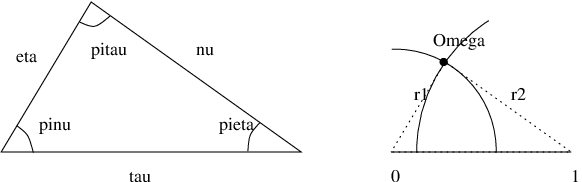
Refer to caption
Figure 3.1: The triangle of (3.3) on the left and its scaled version defined by intersection of circles on the right.

The condition (3.3) is also equivalent to saying that the circle centered at 00 of radius η/τ\sqrt{\eta/\tau} has two disjoint intersections with the circle centered at 11 of radius ν/τ\sqrt{\nu/\tau}. In that case, the two intersections are complex conjugate. Denote by Ω⁡(ν,η,τ)\Omega(\nu,\eta,\tau) the intersection in

ℍ={z∈ℂ|Im⁡(z)>0}.\mathbb{H}=\{z\in\mathbb{C}\,|\,\mathrm{Im}(z)>0\}. (3.4)

Then, we have the following properties

|Ω|2=ητ,|1−Ω|2=ντ,arg⁡(Ω)=πν,arg⁡(1−Ω)=−πη.|\Omega|^{2}=\frac{\eta}{\tau},\quad|1-\Omega|^{2}=\frac{\nu}{\tau},\quad\arg(\Omega)=\pi_{\nu},\quad\arg(1-\Omega)=-\pi_{\eta}. (3.5)

The cosine rule gives the angles π∗\pi_{*}’s in (0,π)(0,\pi) by

πν\displaystyle\pi_{\nu} =\displaystyle= arccos⁡(τ+η−ν2​τ​η),\displaystyle\arccos\left(\frac{\tau+\eta-\nu}{2\sqrt{\tau\eta}}\right),
πη\displaystyle\pi_{\eta} =\displaystyle= arccos⁡(τ+ν−η2​τ​ν),\displaystyle\arccos\left(\frac{\tau+\nu-\eta}{2\sqrt{\tau\nu}}\right), (3.6)
πτ\displaystyle\pi_{\tau} =\displaystyle= arccos⁡(η+ν−η2​ν​η).\displaystyle\arccos\left(\frac{\eta+\nu-\eta}{2\sqrt{\nu\eta}}\right).
Proposition 3.2 (Bulk scaling limit).

For any k=1,2,…k=1,2,\dots, consider

ϰj(L)=(xj(L),nj(L),tj(L)),j=1,…,k,\varkappa_{j}(L)=(x_{j}(L),n_{j}(L),t_{j}(L)),\qquad j=1,\dots,k, (3.7)

such that for any i≠ji\neq j and any L>0L>0 either (ni​(L),ti​(L))≺(nj​(L),tj​(L))(n_{i}(L),t_{i}(L))\prec(n_{j}(L),t_{j}(L)) or (nj​(L),tj​(L))≺(ni​(L),ti​(L))(n_{j}(L),t_{j}(L))\prec(n_{i}(L),t_{i}(L)) (the notation ≺\prec was defined in (1.3)). Assume that

limL→∞xjL=ν,limL→∞njL=η,limL→∞tjL=τ,j=1,…,k;\lim_{L\to\infty}\frac{x_{j}}{L}=\nu,\qquad\lim_{L\to\infty}\frac{n_{j}}{L}=\eta,\qquad\lim_{L\to\infty}\frac{t_{j}}{L}=\tau,\qquad j=1,\dots,k; (3.8)

we have (ν,η,τ)∈𝒟(\nu,\eta,\tau)\in\mathcal{D}; and also all the differences xi−xjx_{i}-x_{j}, ni−njn_{i}-n_{j}, ti−tjt_{i}-t_{j} do not depend on the large parameter LL. Then the kk-point correlation function ρk​(ϰ1,…,ϰk)\rho_{k}(\varkappa_{1},\ldots,\varkappa_{k}) converges to the determinant det[Ki​jbulk]1≤i,j≤k\det[K^{\rm bulk}_{ij}]_{1\leq i,j\leq k}, where

Ki,jbulk=12​π​i​∫1−Ω⁡(ν,η,τ)1−Ω¯​(ν,η,τ)d​w​(1−w)ni−nj​e(tj−ti)​wwxi−xj+1,K^{\rm bulk}_{i,j}=\frac{1}{2\pi{\rm i}}\int_{1-\Omega(\nu,\eta,\tau)}^{1-\overline{\Omega}(\nu,\eta,\tau)}\mathrm{d}w\frac{(1-w)^{n_{i}-n_{j}}e^{(t_{j}-t_{i})w}}{w^{x_{i}-x_{j}+1}}, (3.9)

where for (ni,ti)⊀(nj,tj)(n_{i},t_{i})\not\prec(n_{j},t_{j}) the integration contour crosses ℝ+\mathbb{R}_{+}, while for (ni,ti)≺(nj,tj)(n_{i},t_{i})\prec(n_{j},t_{j}) the contour crosses ℝ−\mathbb{R}_{-}. On the other hand, if (ν,η,τ)∉𝒟(\nu,\eta,\tau)\not\in\mathcal{D}, then

limL→∞ρk​(ϰ1,…,ϰk)=0,\displaystyle\lim_{L\to\infty}\rho_{k}(\varkappa_{1},\ldots,\varkappa_{k})=0, if ​ν>η+τ\displaystyle\textrm{if }\sqrt{\nu}>\sqrt{\eta}+\sqrt{\tau} (3.10)
limL→∞ρk​(ϰ1,…,ϰk)=0,\displaystyle\lim_{L\to\infty}\rho_{k}(\varkappa_{1},\ldots,\varkappa_{k})=0, if ​ν<τ−η\displaystyle\textrm{if }\sqrt{\nu}<\sqrt{\tau}-\sqrt{\eta}
limL→∞ρk​(ϰ1,…,ϰk)=1,\displaystyle\lim_{L\to\infty}\rho_{k}(\varkappa_{1},\ldots,\varkappa_{k})=1, if ​ν<η−τ.\displaystyle\textrm{if }\sqrt{\nu}<\sqrt{\eta}-\sqrt{\tau}.

Proof of Proposition 3.2. One follows exactly the same steps as in Section 3.2 of [41], replacing the double integral (35) in there by (4.2). The deformed paths are then like in Figure 6.4 but with zc=wcz_{c}=w_{c}. The degenerate cases when ϰj∉𝒟\varkappa_{j}\not\in\mathcal{D} are treated in the same way with limiting kernel Ki,jK_{i,j} being either 00 (no residue in the contour integral computation) or triangular (Ki,j=0K_{i,j}=0 for xi<xjx_{i}<x_{j}) with Ki,i=1K_{i,i}=1, when the integral in (3.9) is over a complete circle around the origin. ∎

Corollary 3.3.

Let ρ\rho denote the asymptotic xx-density. Then, in 𝒟\cal D, it is given by

ρ⁡(ν,η,τ)=limL→∞ρ1​([ν​L],[η​L],τ​L)=πη/π∈[0,1].\rho(\nu,\eta,\tau)=\lim_{L\to\infty}\rho_{1}([\nu L],[\eta L],\tau L)=\pi_{\eta}/\pi\in[0,1]. (3.11)

Consequently,

h​(ν,η,τ):=limL→∞𝔼​h​([(ν−η)​L],[η​L],τ​L)L=1π​∫ν(τ+η)2πη​(ν′,η,τ)​d​ν′.\textit{{h}}(\nu,\eta,\tau):=\lim_{L\to\infty}\frac{\mathbbm{E}h([(\nu-\eta)L],[\eta L],\tau L)}{L}=\frac{1}{\pi}\int_{\nu}^{(\sqrt{\tau}+\sqrt{\eta})^{2}}\pi_{\eta}(\nu^{\prime},\eta,\tau)\mathrm{d}\nu^{\prime}. (3.12)

Below we perform the integral in (3.12) to get an explicit expression for the limit shape h. Along the way we derive some interesting geometric relations. First of all, h is homogeneous of degree one (since it is the scaling limit under same scaling in all directions).

Lemma 3.4.

For any α>0\alpha>0,

h​(α​ν,α​η,α​τ)=α​h​(ν,η,τ),\textit{{h}}(\alpha\nu,\alpha\eta,\alpha\tau)=\alpha\textit{{h}}(\nu,\eta,\tau), (3.13)

from which it follows

(ν​∂∂ν+η​∂∂η+τ​∂∂τ)​h​(ν,η,τ)=h​(ν,η,τ).\left(\nu\frac{\partial}{\partial\nu}+\eta\frac{\partial}{\partial\eta}+\tau\frac{\partial}{\partial\tau}\right)\textit{{h}}(\nu,\eta,\tau)=\textit{{h}}(\nu,\eta,\tau). (3.14)

Proof of Lemma 3.4. It follows directly from the geometric property πη​(α​ν,α​η,α​τ)=πη​(ν,η,τ)\pi_{\eta}(\alpha\nu,\alpha\eta,\alpha\tau)=\pi_{\eta}(\nu,\eta,\tau). ∎

Therefore, we just need to compute the partial derivatives of h, then the limit shape h will be determined by the l.h.s. of (3.14).

Proposition 3.5.

The partial derivatives of the limit shape h are given by

∂h∂ν=−πηπ,∂h∂η=1−πνπ,∂h∂τ=sin⁡(πν)​sin⁡(πη)π​sin⁡(πτ).\frac{\partial\textit{{h}}}{\partial\nu}=-\frac{\pi_{\eta}}{\pi},\quad\frac{\partial\textit{{h}}}{\partial\eta}=1-\frac{\pi_{\nu}}{\pi},\quad\frac{\partial\textit{{h}}}{\partial\tau}=\frac{\sin(\pi_{\nu})\sin(\pi_{\eta})}{\pi\sin(\pi_{\tau})}. (3.15)
Remark 3.6.

Another expression for the growth velocity is

∂h∂τ=1π​Im​Ω​(ν,η,τ).\frac{\partial\textit{{h}}}{\partial\tau}=\frac{1}{\pi}\mathrm{Im}\Omega(\nu,\eta,\tau). (3.16)

This can be understood using Proposition 3.2. The macroscopic growth velocity is equal to the average flow of particles, JJ. It is computed in Section 5, see (5.40) with Q=0Q=0: 𝔼(J)=−∂2K(x,n,t;x,n,t)\mathbbm{E}(J)=-\partial_{2}K(x,n,t;x,n,t). Then, by (5.49) we have 𝔼⁡(J)=K⁡(x,n,t,x+1,n,t)\mathbbm{E}(J)=K(x,n,t;x+1,n,t). Finally, by Proposition 3.2 one gets 𝔼⁡(J)=Im​Ω/π\mathbbm{E}(J)=\mathrm{Im}\Omega/\pi.

As a corollary of Lemma 3.4 and Proposition 3.5, the limit shape is given as follows.

Corollary 3.7.

For (ν,η,τ)∈𝒟(\nu,\eta,\tau)\in{\cal D}, we have

h​(ν,η,τ)=1π​(−ν​πη+η⁡(π−πν)+τ​sin⁡(πν)​sin⁡(πη)sin⁡(πτ)).\textit{{h}}(\nu,\eta,\tau)=\frac{1}{\pi}\left(-\nu\pi_{\eta}+\eta(\pi-\pi_{\nu})+\tau\frac{\sin(\pi_{\nu})\sin(\pi_{\eta})}{\sin(\pi_{\tau})}\right). (3.17)

Proof of Proposition 3.5. From (3.12) we immediately have the first relation: ∂h/∂ν=−πη/π\partial\textit{{h}}/\partial\nu=-\pi_{\eta}/\pi. In the derivatives of h with respect to τ\tau and η\eta we have one term coming from the boundary term and one from the internal derivative. The boundary terms will actually be zero, since the density at the upper edge is zero. We need to compute

∂πη∂η=14​η​τ−(ν−η−τ)2,∂πη∂τ=ν−η−τ2​τ​4​η​τ−(ν−η−τ)2.\frac{\partial\pi_{\eta}}{\partial\eta}=\frac{1}{\sqrt{4\eta\tau-(\nu-\eta-\tau)^{2}}},\quad\frac{\partial\pi_{\eta}}{\partial\tau}=\frac{\nu-\eta-\tau}{2\tau\sqrt{4\eta\tau-(\nu-\eta-\tau)^{2}}}. (3.18)

Then, we apply the indefinite integrals

∫d​xa2−x2=arcsin⁡(x/|a|)+C,∫x​d​xa2−x2=−a2−x2+C.\int\frac{\mathrm{d}x}{a^{2}-x^{2}}=\arcsin(x/|a|)+C,\quad\int\frac{x\mathrm{d}x}{\sqrt{a^{2}-x^{2}}}=-\sqrt{a^{2}-x^{2}}+C. (3.19)

For the derivative with respect to η\eta,

π​∂h∂η\displaystyle\pi\frac{\partial\textit{{h}}}{\partial\eta} =\displaystyle= ∫ν(η+τ)2∂πη∂η​d​ν′+(1+τ/η)​πη​((η+τ)2,η,τ)\displaystyle\int_{\nu}^{(\sqrt{\eta}+\sqrt{\tau})^{2}}\frac{\partial\pi_{\eta}}{\partial\eta}\mathrm{d}\nu^{\prime}+(1+\sqrt{\tau/\eta})\pi_{\eta}\left((\sqrt{\eta}+\sqrt{\tau})^{2},\eta,\tau\right) (3.20)
=\displaystyle= π/2+arcsin⁡(η+τ−ν2​η​τ)=π−arccos⁡(η+τ−ν2​η​τ),\displaystyle\pi/2+\arcsin\left(\frac{\eta+\tau-\nu}{2\sqrt{\eta\tau}}\right)=\pi-\arccos\left(\frac{\eta+\tau-\nu}{2\sqrt{\eta\tau}}\right),

the latter being πν\pi_{\nu}. Finally,

π​∂h∂τ\displaystyle\pi\frac{\partial\textit{{h}}}{\partial\tau} =\displaystyle= ∫ν(η+τ)2∂πη∂τ​d​ν′+(1+η/τ)​πη​((η+τ)2,η,τ)\displaystyle\int_{\nu}^{(\sqrt{\eta}+\sqrt{\tau})^{2}}\frac{\partial\pi_{\eta}}{\partial\tau}\mathrm{d}\nu^{\prime}+(1+\sqrt{\eta/\tau})\pi_{\eta}\left((\sqrt{\eta}+\sqrt{\tau})^{2},\eta,\tau\right) (3.21)
=\displaystyle= 4​η​τ−(ν−η−τ)22​τ=η/τ​sin⁡(πν),\displaystyle\frac{\sqrt{4\eta\tau-(\nu-\eta-\tau)^{2}}}{2\tau}=\sqrt{\eta/\tau}\sin(\pi_{\nu}),

and by the sinus theorem for the triangle of Figure 3.1 we have η/τ=sin⁡(πη)/sin⁡(πτ)\sqrt{\eta}/\sqrt{\tau}=\sin(\pi_{\eta})/\sin(\pi_{\tau}). ∎

Refer to caption
Refer to caption
Figure 3.2: (a) Limiting density of the particles with τ=1\tau=1. (b) The associated limiting height function. Two facets are visible.

3.2 Growth model in the anisotropic KPZ class

For fixed τ\tau, the macroscopic slopes of the interface in the ν\nu- and η\eta-directions are given by hν:=∂νh\textit{{h}}_{\nu}:=\partial_{\nu}\textit{{h}} and hη:=∂ηh\textit{{h}}_{\eta}:=\partial_{\eta}\textit{{h}}. The speed of growth of the surface, ∂τh\partial_{\tau}\textit{{h}}, depends only on these two slopes. Indeed, by (3.15), we can rewrite

v=∂h∂τ=−1π​sin⁡(π​hν)​sin⁡(π​hη)sin⁡(π⁡(hν+hη)).v=\frac{\partial\textit{{h}}}{\partial\tau}=-\frac{1}{\pi}\frac{\sin(\pi\textit{{h}}_{\nu})\sin(\pi\textit{{h}}_{\eta})}{\sin(\pi(\textit{{h}}_{\nu}+\textit{{h}}_{\eta}))}. (3.22)

Remark that the speed of growth is monotonically decreasing with the slope

∂v⁡(hν,hη)∂hν<0,∂v⁡(hν,hη)∂hη<0\frac{\partial v(\textit{{h}}_{\nu},\textit{{h}}_{\eta})}{\partial\textit{{h}}_{\nu}}<0,\quad\frac{\partial v(\textit{{h}}_{\nu},\textit{{h}}_{\eta})}{\partial\textit{{h}}_{\eta}}<0 (3.23)

for hν,hη,hν+hη∈(0,1)\textit{{h}}_{\nu},\textit{{h}}_{\eta},\textit{{h}}_{\nu}+\textit{{h}}_{\eta}\in(0,1).

To see which universality class our model belongs to, we need to compute the determinant of the Hessian of v=v⁡(hν,hη)v=v(\textit{{h}}_{\nu},\textit{{h}}_{\eta}). Explicit computations give

|∂hν∂hνv∂hν∂hηv∂hη∂hνv∂hη∂hηv|=−4​π2​sin(πhν)2sin(πhη)2sin⁡(π⁡(hν+hη))4<0\left|\begin{array}[]{cc}\partial_{\textit{{h}}_{\nu}}\partial_{\textit{{h}}_{\nu}}v&\partial_{\textit{{h}}_{\nu}}\partial_{\textit{{h}}_{\eta}}v\\ \partial_{\textit{{h}}_{\eta}}\partial_{\textit{{h}}_{\nu}}v&\partial_{\textit{{h}}_{\eta}}\partial_{\textit{{h}}_{\eta}}v\end{array}\right|=-4\pi^{2}\frac{\sin(\pi\textit{{h}}_{\nu})^{2}\sin(\pi\textit{{h}}_{\eta})^{2}}{\sin(\pi(\textit{{h}}_{\nu}+\textit{{h}}_{\eta}))^{4}}<0 (3.24)

for hν,hη,hν+hη∈(0,1)\textit{{h}}_{\nu},\textit{{h}}_{\eta},\textit{{h}}_{\nu}+\textit{{h}}_{\eta}\in(0,1), i.e., for (ν,η,τ)∈𝒟(\nu,\eta,\tau)\in{\cal D}. Thus, our model belongs to the anisotropic KPZ universality class of growth models in 2+12+1 dimensions.

3.3 A few other geometric properties

During the asymptotic analysis we will use a few more geometric quantities, which we collect in this section. The key function to be analyzed is

G⁡(w)≡G⁡(w|ν,η,τ)=τ​w+ν​ln⁡(1−w)−η​ln⁡(w),w∈ℂ.G(w)\equiv G(w|\nu,\eta,\tau)=\tau w+\nu\ln(1-w)-\eta\ln(w),\quad w\in\mathbb{C}. (3.25)

The critical points of GG coincide with Ω\Omega as stated below.

Proposition 3.8.

On ℂ∖{0,1}\mathbb{C}\setminus\{0,1\}, the function GG has two critical points (counted with multiplicities). These two points are distinct and complex conjugate if and only if (ν,η,τ)∈𝒟(\nu,\eta,\tau)\in{\cal D}, in which case the critical points are {Ω,Ω¯}\{\Omega,\overline{\Omega}\}.

Proof of Proposition 3.8. The derivative of GG gives

G′​(w)=τw⁡(w−1)​((w−η+τ−ν2​τ)2+4​η​τ−(η+τ−ν)24​τ2),G^{\prime}(w)=\frac{\tau}{w(w-1)}\left(\left(w-\frac{\eta+\tau-\nu}{2\tau}\right)^{2}+\frac{4\eta\tau-(\eta+\tau-\nu)^{2}}{4\tau^{2}}\right), (3.26)

and we have two distinct complex conjugate solutions iff 4​η​τ−(η+τ−ν)2>04\eta\tau-(\eta+\tau-\nu)^{2}>0, i.e., iff (ν,η,τ)∈𝒟(\nu,\eta,\tau)\in{\cal D}. Also, from (3.5) and (3.6) we get

Re⁡(Ω)=η+τ−ν2​τ,Im⁡(Ω)=4​η​τ−(η+τ−ν)22​τ.\mathrm{Re}(\Omega)=\frac{\eta+\tau-\nu}{2\tau},\quad\mathrm{Im}(\Omega)=\frac{\sqrt{4\eta\tau-(\eta+\tau-\nu)^{2}}}{2\tau}. (3.27)

Thus, Ω\Omega and Ω¯\overline{\Omega} are the two solutions of G′​(w)=0G^{\prime}(w)=0, i.e., the two critical points. ∎

The main formulas needed later are the partial derivatives of Ω\Omega as well as G′′​(Ω)G^{\prime\prime}(\Omega).

Proposition 3.9.

Denote κ=2​τ​Im​(Ω)=4​η​τ−(η+τ−ν)2\kappa=2\tau\mathrm{Im}(\Omega)=\sqrt{4\eta\tau-(\eta+\tau-\nu)^{2}}. Then we have

G′′​(Ω)=−i​κΩ⁡(1−Ω),G^{\prime\prime}(\Omega)=\frac{-{\rm i}\kappa}{\Omega(1-\Omega)}, (3.28)

which implies

|G′′​(Ω)|=κ|Ω⁡(1−Ω)|,arg⁡(G′′​(Ω))=−π2−πν+πη.|G^{\prime\prime}(\Omega)|=\frac{\kappa}{|\Omega(1-\Omega)|},\quad\arg(G^{\prime\prime}(\Omega))=-\frac{\pi}{2}-\pi_{\nu}+\pi_{\eta}. (3.29)

Moreover,

∂Ω∂ν=i​Ωκ,∂Ω∂η=i⁡(1−Ω)κ,∂Ω∂τ=−i​Ω​(1−Ω)κ.\frac{\partial\Omega}{\partial\nu}=\frac{{\rm i}\Omega}{\kappa},\quad\frac{\partial\Omega}{\partial\eta}=\frac{{\rm i}(1-\Omega)}{\kappa},\quad\frac{\partial\Omega}{\partial\tau}=\frac{-{\rm i}\Omega(1-\Omega)}{\kappa}. (3.30)

Proof of Proposition 3.9. From (3.26) we get

G′′​(Ω)=2​τΩ⁡(Ω−1)​(Ω−Re⁡(Ω))=2​i​τ​Im​(Ω)Ω⁡(Ω−1).G^{\prime\prime}(\Omega)=\frac{2\tau}{\Omega(\Omega-1)}(\Omega-\mathrm{Re}(\Omega))=\frac{2{\rm i}\tau\mathrm{Im}(\Omega)}{\Omega(\Omega-1)}. (3.31)

The modulus is immediate, while the argument is obtained using (3.5).

Since Ω\Omega is the intersection point of the circles |z|=η/τ|z|=\sqrt{\eta/\tau} and |1−z|=ν/τ|1-z|=\sqrt{\nu/\tau}, the direction of ∂νΩ\partial_{\nu}\Omega is orthogonal to the vector Ω\Omega and ∂ηΩ\partial_{\eta}\Omega is orthogonal to 1−Ω1-\Omega. Therefore, for some c1,c2∈ℝc_{1},c_{2}\in\mathbb{R},

∂Ω∂ν=c1​Ω​i,∂Ω∂η=c2​(1−Ω)​i.\frac{\partial\Omega}{\partial\nu}=c_{1}\Omega{\rm i},\quad\frac{\partial\Omega}{\partial\eta}=c_{2}(1-\Omega){\rm i}. (3.32)

Looking at the real part of these equations, we get ∂νRe⁡(Ω)=−c1​Im​(Ω)\partial_{\nu}\mathrm{Re}(\Omega)=-c_{1}\mathrm{Im}(\Omega), and ∂νRe⁡(Ω)=c2​Im​(Ω)\partial_{\nu}\mathrm{Re}(\Omega)=c_{2}\mathrm{Im}(\Omega). On the other hand,

Re⁡(Ω)=η+τ−ν2​τ⇒∂νRe⁡(Ω)=−12​τ,∂ηRe⁡(Ω)=12​τ.\mathrm{Re}(\Omega)=\frac{\eta+\tau-\nu}{2\tau}\quad\Rightarrow\quad\partial_{\nu}\mathrm{Re}(\Omega)=-\frac{1}{2\tau},\quad\partial_{\eta}\mathrm{Re}(\Omega)=\frac{1}{2\tau}. (3.33)

From this we conclude that

∂νΩ=i​Ω2​τ​Im​(Ω),∂ηΩ=i⁡(1−Ω)2​τ​Im​(Ω).\partial_{\nu}\Omega=\frac{{\rm i}\Omega}{2\tau\mathrm{Im}(\Omega)},\quad\partial_{\eta}\Omega=\frac{{\rm i}(1-\Omega)}{2\tau\mathrm{Im}(\Omega)}. (3.34)

To get ∂τΩ\partial_{\tau}\Omega, we can use the following property: Ω⁡(a​ν,a​η,a​τ)=Ω⁡(ν,η,τ)\Omega(a\nu,a\eta,a\tau)=\Omega(\nu,\eta,\tau) for any a>0a>0, which implies

(ν∂ν+η∂η+τ∂τ)Ω=0.\left(\nu\partial_{\nu}+\eta\partial_{\eta}+\tau\partial_{\tau}\right)\Omega=0. (3.35)

This equation leads to

∂τΩ=−i2​τ​Im​(Ω)​(ντ​Ω+ητ​(1−Ω))=−i​Ω​(1−Ω)2​τ​Im​(Ω),\partial_{\tau}\Omega=-\frac{{\rm i}}{2\tau\mathrm{Im}(\Omega)}\left(\frac{\nu}{\tau}\Omega+\frac{\eta}{\tau}(1-\Omega)\right)=-\frac{{\rm i}\Omega(1-\Omega)}{2\tau\mathrm{Im}(\Omega)}, (3.36)

using |Ω|2=η/τ|\Omega|^{2}=\eta/\tau and |1−Ω|2=ν/τ|1-\Omega|^{2}=\nu/\tau, see (3.5). ∎

Another important function appearing in the asymptotics of the kernel is the imaginary part of G⁡(Ω)G(\Omega) (and its derivatives).

Proposition 3.10.

We have

γ⁡(ν,η,τ):=Im⁡(G⁡(Ω))=τ​Im​(Ω)−ν​πη−η​πν,\gamma(\nu,\eta,\tau):=\mathrm{Im}(G(\Omega))=\tau\mathrm{Im}(\Omega)-\nu\pi_{\eta}-\eta\pi_{\nu}, (3.37)

Its derivatives are

∂Im⁡(G⁡(Ω))∂ν=−πη,∂Im⁡(G⁡(Ω))∂η=−πν,\frac{\partial\mathrm{Im}(G(\Omega))}{\partial\nu}=-\pi_{\eta},\quad\frac{\partial\mathrm{Im}(G(\Omega))}{\partial\eta}=-\pi_{\nu}, (3.38)

and

∂2Im⁡(G⁡(Ω))∂ν​∂η=−1κ,κ=2​τ​Im​(Ω).\frac{\partial^{2}\mathrm{Im}(G(\Omega))}{\partial\nu\partial\eta}=-\frac{1}{\kappa},\quad\kappa=2\tau\mathrm{Im}(\Omega). (3.39)

Proof of Proposition 3.10. The relation (3.37) is a direct consequence of (3.5). The rest are just simple computations. ∎

4 Gaussian fluctuations

In this section we first state a couple of equivalent forms of the correlation kernel. In particular, the kernel for a fixed (n,t)(n,t) has a Christoffel-Darboux representation in terms of Charlier polynomials. In the second part of the section we prove Theorem 1.2 on the Gaussian fluctuations.

4.1 Kernel representations

For the analysis of the variance we will use a representation in terms of Charlier polynomials. These polynomials are defined on ℤ+={0,1,2,…}\mathbb{Z}_{+}=\{0,1,2,\ldots\}, while our particles at level nn live on {−n,−n+1,…}\{-n,-n+1,\ldots\}. Thus, it is convenient to shift the position at level nn by nn, i.e., the positions of particles at level nn will be denoted by −n+x-n+x, x≥0x\geq 0. Finally, we also conjugate by a factor (−1)n1−n2(-1)^{n_{1}-n_{2}}. More precisely, the relation between the shifted and conjugate kernel KK and the kernel 𝒦\cal K in Theorem 1.1, is the following,

K⁡(x1,n1,t1,x2,n2,t2)=(−1)n1−n2​𝒦​(x1−n1,n1,t1,x2−n2,n2,t2).K(x_{1},n_{1},t_{1};x_{2},n_{2},t_{2})=(-1)^{n_{1}-n_{2}}{\cal K}(x_{1}-n_{1},n_{1},t_{1};x_{2}-n_{2},n_{2},t_{2}). (4.1)

For later use, we give the explicit double integral representation of KK which will be used in the asymptotic analysis.

Corollary 4.1.

The extended kernel KK can be expressed as

K⁡(x1,n1,t1,x2,n2,t2)={et1−t2(2​π​i)2​∮Γ1d​z​∮Γ0d​w​zn1et1​z​(1−z)x1+1​et2​w​(1−w)x2wn2​1w−z,(n1,t1)⊀(n2,t2)et1−t2(2​π​i)2​∮Γ1d​z​∮Γ0,zd​w​zn1et1​z​(1−z)x1+1​et2​w​(1−w)x2wn2​1w−z,(n1,t1)≺(n2,t2)K(x_{1},n_{1},t_{1};x_{2},n_{2},t_{2})\\ =\begin{cases}\frac{e^{t_{1}-t_{2}}}{(2\pi{\rm i})^{2}}\oint_{\Gamma_{1}}\mathrm{d}z\oint_{\Gamma_{0}}\mathrm{d}w\frac{z^{n_{1}}}{e^{t_{1}z}(1-z)^{x_{1}+1}}\frac{e^{t_{2}w}(1-w)^{x_{2}}}{w^{n_{2}}}\frac{1}{w-z},&(n_{1},t_{1})\not\prec(n_{2},t_{2})\\[5.0pt] \frac{e^{t_{1}-t_{2}}}{(2\pi{\rm i})^{2}}\oint_{\Gamma_{1}}\mathrm{d}z\oint_{\Gamma_{0,z}}\mathrm{d}w\frac{z^{n_{1}}}{e^{t_{1}z}(1-z)^{x_{1}+1}}\frac{e^{t_{2}w}(1-w)^{x_{2}}}{w^{n_{2}}}\frac{1}{w-z},&(n_{1},t_{1})\prec(n_{2},t_{2})\end{cases} (4.2)

Proof of Corollary 4.1. The kernel (4.2) is obtained by substituting into (4.1) the expression for 𝒦\cal K from (1.6), and applying the change of variables z→1/(1−w)z\to 1/(1-w) and w→1/(1−z)w\to 1/(1-z). ∎

It is instructive to see the structure of the kernel that leads the above integral representation.

Proposition 4.2.

The extended kernel KK is given by

K⁡(x1,n1,t1,x1,n2,t2)=−ϕ((n1,t1),(n2,t2))​(x1,x2)+∑k=1n2Ψn1−kn1,t1​(x1)​Φn2−kn2,t2​(x2)K(x_{1},n_{1},t_{1};x_{1},n_{2},t_{2})=-\phi^{((n_{1},t_{1}),(n_{2},t_{2}))}(x_{1},x_{2})+\sum_{k=1}^{n_{2}}\Psi^{n_{1},t_{1}}_{n_{1}-k}(x_{1})\Phi^{n_{2},t_{2}}_{n_{2}-k}(x_{2}) (4.3)

with

Ψkn,t​(x)\displaystyle\Psi^{n,t}_{k}(x) =\displaystyle= 12​π​i​∮Γ0,1d​w​et​w​(1−w)kwx+1,\displaystyle\frac{1}{2\pi{\rm i}}\oint_{\Gamma_{0,1}}\mathrm{d}w\frac{e^{tw}(1-w)^{k}}{w^{x+1}},
Φkn,t​(x)\displaystyle\Phi^{n,t}_{k}(x) =\displaystyle= −12​π​i​∮Γ1d​z​zx​e−t​z(1−z)k+1,\displaystyle\frac{-1}{2\pi{\rm i}}\oint_{\Gamma_{1}}\mathrm{d}z\frac{z^{x}e^{-tz}}{(1-z)^{k+1}}, (4.4)
ϕ((n1,t1),(n2,t2))​(x1,x2)\displaystyle\phi^{((n_{1},t_{1}),(n_{2},t_{2}))}(x_{1},x_{2}) =\displaystyle= 12​π​i∮Γ0,1dwew⁡(t1−t2)wx1−x2+1​(w−1)n2−n1𝟙[(n1,t1)≺(n2,t2)],\displaystyle\frac{1}{2\pi{\rm i}}\oint_{\Gamma_{0,1}}\mathrm{d}w\frac{e^{w(t_{1}-t_{2})}}{w^{x_{1}-x_{2}+1}(w-1)^{n_{2}-n_{1}}}\mathbbm{1}_{[(n_{1},t_{1})\prec(n_{2},t_{2})]},

where Γ0,1\Gamma_{0,1} and Γ1\Gamma_{1} are any simple anticlockwise oriented contours that include poles {0,1}\{0,1\} and {1}\{1\}, respectively.

Proof of Proposition 4.2. Using the integral representations for Ψ\Psi and Φ\Phi one checks that

∑k≥0Ψkn1,t1​(x)​Φkn2,t2​(y)=ϕ((n1,t1),(n2,t2))​(x,y).\sum_{k\geq 0}\Psi^{n_{1},t_{1}}_{k}(x)\Phi^{n_{2},t_{2}}_{k}(y)=\phi^{((n_{1},t_{1}),(n_{2},t_{2}))}(x,y). (4.5)

Thus (4.3) becomes

K⁡(x1,n1,t1,x2,n2,t2)={∑k=1n2Ψn1−kn1,t1​(x1)​Φn2−kn2,t2​(x2),(n1,t1)⊀(n2,t2)−∑l=0∞Ψn1,t1n1+l(x1)Φn2,t2n2+l(x2),(n1,t1)≺(n2,t2)K(x_{1},n_{1},t_{1};x_{2},n_{2},t_{2})=\left\{\begin{array}[]{ll}\sum_{k=1}^{n_{2}}\Psi^{n_{1},t_{1}}_{n_{1}-k}(x_{1})\Phi^{n_{2},t_{2}}_{n_{2}-k}(x_{2}),&(n_{1},t_{1})\not\prec(n_{2},t_{2})\\[5.0pt] -\sum_{l=0}^{\infty}\Psi^{n_{1},t_{1}}_{n_{1}+l}(x_{1})\Phi^{n_{2},t_{2}}_{n_{2}+l}(x_{2}),&(n_{1},t_{1})\prec(n_{2},t_{2})\end{array}\right. (4.6)

This new expression is good because in (4.4) we never have the case when the pole at w=1w=1 in Ψkn,t\Psi^{n,t}_{k} survives. Then, one has just to take the sums inside the integral. For example, for (n1,t1)⊀(n2,t2)(n_{1},t_{1})\not\prec(n_{2},t_{2}), we first take the sum inside the integrals and then we extend it to k=∞k=\infty. This can be done provided |1−w|>|1−z||1-w|>|1-z|. Then, to get the formula (4.2), one just has to rename the variables z→1−wz\to 1-w and w→1−zw\to 1-z. ∎

For the computation of the variance, we will need only the kernel at fixed (n,t)(n,t). It is given in terms of the Charlier polynomials, Cn​(x,t)C_{n}(x,t), given by

Cn​(x,t)=n!tn​12​π​i​∮Γ0d​w​(1−w)x​ew​twn+1,C_{n}(x,t)=\frac{n!}{t^{n}}\frac{1}{2\pi{\rm i}}\oint_{\Gamma_{0}}\mathrm{d}w\frac{(1-w)^{x}e^{wt}}{w^{n+1}}, (4.7)

which satisfy Cn​(x,t)=Cx​(n,t)C_{n}(x,t)=C_{x}(n,t), and are orthogonal with respect to the weight wt​(x)=e−t​txx!w_{t}(x)=\frac{e^{-t}t^{x}}{x!}, namely

∑x≥0Cn​(x,t)​Cm​(x,t)​wt​(x)=n!tn​δn,m,t>0.\sum_{x\geq 0}C_{n}(x,t)C_{m}(x,t)w_{t}(x)=\frac{n!}{t^{n}}\delta_{n,m},\quad t>0. (4.8)
Corollary 4.3.

The kernel K⁡(x,n,t,y,n,t)K(x,n,t;y,n,t) is equivalent (conjugate) to the kernel Kn,t​(x,y)K_{n,t}(x,y), given by

Kn,t​(x,y)=n​t​qn−1​(x,t)​qn​(y,t)−qn​(x,t)​qn−1​(y,t)x−y,K_{n,t}(x,y)=\sqrt{nt}\frac{q_{n-1}(x,t)q_{n}(y,t)-q_{n}(x,t)q_{n-1}(y,t)}{x-y}, (4.9)

where

qn​(x,t)=wt​(x)1/2​tn/2n!​Cn​(x,t),q_{n}(x,t)=w_{t}(x)^{1/2}\frac{t^{n/2}}{\sqrt{n!}}C_{n}(x,t), (4.10)

Proof of Corollary 4.3. Consider n1=n2=nn_{1}=n_{2}=n and t1=t2=tt_{1}=t_{2}=t in (4.3). Then,

K⁡(x,n,t,y,n,t)=∑k=0n−1Ψkn,t​(x)​Φkn,t​(y).K(x,n,t;y,n,t)=\sum_{k=0}^{n-1}\Psi^{n,t}_{k}(x)\Phi^{n,t}_{k}(y). (4.11)

For all k≥0k\geq 0, w=1w=1 is not a pole in the integral representation of Ψkn,t\Psi^{n,t}_{k}. Using (4.7) and Cn​(x,t)=Cx​(n,t)C_{n}(x,t)=C_{x}(n,t), we get Ψkn,t​(x)=txx!​Ck​(x,t)\Psi^{n,t}_{k}(x)=\frac{t^{x}}{x!}C_{k}(x,t). Also, by the change of variable z→1−wz\to 1-w in the integral representation Φkn,t\Phi^{n,t}_{k} we obtain Φkn,t​(x)=e−t​tkk!​Ck​(x,t)\Phi^{n,t}_{k}(x)=e^{-t}\frac{t^{k}}{k!}C_{k}(x,t). Thus the kernel writes

K⁡(x,n,t,y,n,t)=wt​(x)​∑k=0n−1tkk!​Ck​(x,t)​Ck​(y,t),K(x,n,t;y,n,t)=w_{t}(x)\sum_{k=0}^{n-1}\frac{t^{k}}{k!}C_{k}(x,t)C_{k}(y,t), (4.12)

which is conjugate to the kernel

Kn,t​(x,y)=∑k=0n−1qk​(x,t)​qk​(y,t).K_{n,t}(x,y)=\sum_{k=0}^{n-1}q_{k}(x,t)q_{k}(y,t). (4.13)

From Cn​(x,t)=un​xn+⋯C_{n}(x,t)=u_{n}x^{n}+\cdots with un=1/(−t)nu_{n}=1/(-t)^{n}, we have qn​(x,t)=vn​xn+⋯q_{n}(x,t)=v_{n}x^{n}+\cdots with vn=(−1)n/tn​n!v_{n}=(-1)^{n}/\sqrt{t^{n}n!}. Then, (4.9) follows from Christoffel-Darboux formula. ∎

Remark 4.4.

For later use, we rewrite qnq_{n} as

qn​(x,t)=Bn,t​(x)​In,t​(x),Bn,t​(x)=e−t/2tx/2x!​n!tn/2,q_{n}(x,t)=B_{n,t}(x)I_{n,t}(x),\quad B_{n,t}(x)=\frac{e^{-t/2}t^{x/2}}{\sqrt{x!}}\frac{\sqrt{n!}}{t^{n/2}}, (4.14)

and

In,t​(x)=12​π​i​∮Γ0d​w​(1−w)x​ew​twn+1.I_{n,t}(x)=\frac{1}{2\pi{\rm i}}\oint_{\Gamma_{0}}\mathrm{d}w\frac{(1-w)^{x}e^{wt}}{w^{n+1}}. (4.15)

4.2 Proof of Theorem 1.2

In this section we look only at the height function at a given time. Therefore, it is convenient to set λ=ν/τ\lambda=\nu/\tau and c=η/τc=\eta/\tau so that we have n=[η​L]=[c​t]n=[\eta L]=[ct] and x=[ν​L]=[λ​t]x=[\nu L]=[\lambda t]. In these variables, the equation for the bulk region given by (3.3) rewrites as

(1−c)2<λ<(1+c)2.(1-\sqrt{c})^{2}<\lambda<(1+\sqrt{c})^{2}. (4.16)

First we compute the variance of the height.

Proposition 4.5.

For any λ∈((1−c)2,(c+1)2)\lambda\in((1-\sqrt{c})^{2},(\sqrt{c}+1)^{2}),

limt→∞Var(h⁡([(λ−c)​t],[c​t],t))ln⁡(t)=12​π2.\lim_{t\to\infty}\frac{\Var(h([(\lambda-c)t],[ct],t))}{\ln(t)}=\frac{1}{2\pi^{2}}. (4.17)

With this we can prove Theorem 1.2.

Proof of Theorem 1.2. It is a consequence of Proposition 4.5 and [50]. More precisely, in Section 2 of [50] the convergence in distribution (a generalization of the result for the sine kernel of [18]) is stated. However, following the proof of the theorem, one realizes that it is done by controlling the cumulants, i.e., also the moments converge. ∎

Proof of Proposition 4.5. The variance can be written in terms of the one and two point correlation functions ρ1\rho_{1} and ρ2\rho_{2}. Namely,

Var(h⁡([(λ−c)​t],[c​t],t))=∑x,y>[λ​t]ρ2​(x,y)+∑x>[λ​t]ρ1​(x)−(∑x>[λ​t]ρ1​(x))2,\Var(h([(\lambda-c)t],[ct],t))=\sum_{x,y>[\lambda t]}\rho_{2}(x,y)+\sum_{x>[\lambda t]}\rho_{1}(x)-\Big(\sum_{x>[\lambda t]}\rho_{1}(x)\Big)^{2}, (4.18)

where ρ2​(x,y)=Kn,t​(x,x)​Kn,t​(y,y)−Kn,t​(x,y)​Kn,t​(y,x)\rho_{2}(x,y)=K_{n,t}(x,x)K_{n,t}(y,y)-K_{n,t}(x,y)K_{n,t}(y,x) and ρ1​(x)=Kn,t​(x,x)\rho_{1}(x)=K_{n,t}(x,x). Using Kn,t2=Kn,tK_{n,t}^{2}=K_{n,t} on ℓ2​(ℤ+)\ell_{2}(\mathbb{Z}_{+}), we have

Var(h⁡([(λ−c)​t],[c​t],t))=∑x>[λ​t]Kn,t​(x,x)−∑x,y>[λ​t]Kn,t​(x,y)​Kn,t​(y,x)\displaystyle\Var(h([(\lambda-c)t],[ct],t))=\sum_{x>[\lambda t]}K_{n,t}(x,x)-\sum_{x,y>[\lambda t]}K_{n,t}(x,y)K_{n,t}(y,x) (4.19)
=∑x>[λ​t]∑y=0∞Kn,t​(x,y)​Kn,t​(y,x)−∑x,y>[λ​t]Kn,t​(x,y)​Kn,t​(y,x)\displaystyle=\sum_{x>[\lambda t]}\sum_{y=0}^{\infty}K_{n,t}(x,y)K_{n,t}(y,x)-\sum_{x,y>[\lambda t]}K_{n,t}(x,y)K_{n,t}(y,x)
=∑x>[λ​t]∑y≤[λ​t](Kn,t(x,y))2,n=[ct].\displaystyle=\sum_{x>[\lambda t]}\sum_{y\leq[\lambda t]}\left(K_{n,t}(x,y)\right)^{2},\qquad n=[ct].

We use the expression (4.9) for the kernel Kn,tK_{n,t}. We decompose the sum in (4.19) into the following three sets:

M\displaystyle M =\displaystyle= {x,y∈ℤ+2|x>[λt],y≤[λt],y−x≤ε1t},\displaystyle\{x,y\in\mathbb{Z}_{+}^{2}|x>[\lambda t],y\leq[\lambda t],y-x\leq\varepsilon_{1}t\},
R1\displaystyle R_{1} =\displaystyle= {x,y∈ℤ+2|x>[λt],y≤[λt],ε1t<y−x<ε2t},\displaystyle\{x,y\in\mathbb{Z}_{+}^{2}|x>[\lambda t],y\leq[\lambda t],\varepsilon_{1}t<y-x<\varepsilon_{2}t\}, (4.20)
R2\displaystyle R_{2} =\displaystyle= {x,y∈ℤ+2|x>[λt],y≤[λt],ε2t≤y−x},\displaystyle\{x,y\in\mathbb{Z}_{+}^{2}|x>[\lambda t],y\leq[\lambda t],\varepsilon_{2}t\leq y-x\},

where the parameter ε2=12​min⁡{(1+c)2−λ,λ−(1−c)2}\varepsilon_{2}=\frac{1}{2}\min\{(1+\sqrt{c})^{2}-\lambda,\lambda-(1-\sqrt{c})^{2}\} is chosen so that R1R_{1} is a subset of the bulk. Thus

Var(h⁡([(λ−c)​t],[c​t],t))=Mt+Rt,1+Rt,2,\Var(h([(\lambda-c)t],[ct],t))=M_{t}+R_{t,1}+R_{t,2}, (4.21)

with

Mt=∑x,y∈M|Kn,t​(x,y)|2,Rt,k=∑x,y∈Rk|Kn,t​(x,y)|2.M_{t}=\sum_{x,y\in M}\left|K_{n,t}(x,y)\right|^{2},\quad R_{t,k}=\sum_{x,y\in R_{k}}\left|K_{n,t}(x,y)\right|^{2}. (4.22)

Remark: The parameter ε1\varepsilon_{1}, small, will be chosen tt-dependent in the end.

(1) Bound on Rt,2R_{t,2}. For x,y∈R2x,y\in R_{2}, we use y−x≥ε2​ty-x\geq\varepsilon_{2}t, and extend the sum to infinities

Rt,2\displaystyle R_{t,2} ≤\displaystyle\leq 1ε22∑x≥λ​t∑y≤λ​t(|q[c​t](x,t)|2|q[c​t]−1(y,t)|2+|q[c​t]−1(x,t)|2|q[c​t](y,t)|2|\displaystyle\frac{1}{\varepsilon_{2}^{2}}\sum_{x\geq\lambda t}\sum_{y\leq\lambda t}\big(|q_{[ct]}(x,t)|^{2}|q_{[ct]-1}(y,t)|^{2}+|q_{[ct]-1}(x,t)|^{2}|q_{[ct]}(y,t)|^{2}| (4.23)
OPEN+2​|q[c​t]−1​(x,t)​q[c​t]​(x,t)|​|q[c​t]−1​(y,t)​q[c​t]​(y,t)|)≤4ε22.\displaystyle+2|q_{[ct]-1}(x,t)q_{[ct]}(x,t)||q_{[ct]-1}(y,t)q_{[ct]}(y,t)|\big)\leq\frac{4}{\varepsilon_{2}^{2}}.

The last inequality follows from Cauchy-Schwarz and the property

∑x≥0|qk​(x,t)|2=⟨Ψkn,t,Φkn,t⟩=1,for all ​k.\sum_{x\geq 0}|q_{k}(x,t)|^{2}=\langle\Psi^{n,t}_{k},\Phi^{n,t}_{k}\rangle=1,\quad\textrm{for all }k. (4.24)

(2) Bound on Rt,1R_{t,1}. Since this time x,y∈R1x,y\in R_{1} are always in the bulk, we just use the bound of Lemma 6.8 and get

Rt,1\displaystyle R_{t,1} ≤\displaystyle\leq const​∑x,y∈R11(x−y)2=const​∑z=[ε1​t][ε2​t]1z\displaystyle\mathrm{const\,}\sum_{x,y\in R_{1}}\frac{1}{(x-y)^{2}}=\mathrm{const\,}\sum_{z=[\varepsilon_{1}t]}^{[\varepsilon_{2}t]}\frac{1}{z} (4.25)
=\displaystyle= Ψ⁡([ε2​t]+1)−Ψ⁡([ε1​t]),\displaystyle\Psi([\varepsilon_{2}t]+1)-\Psi([\varepsilon_{1}t]),

where Ψ⁡(x)\Psi(x) is the digamma function, which has the Taylor expansion at infinity given by

Ψ⁡(x)=ln⁡(x)−1/(2​x)+𝒪⁡(1/x2).\Psi(x)=\ln(x)-1/(2x)+\mathcal{O}(1/x^{2}). (4.26)

Thus

Rt,1≤const​ln⁡(1/ε1),R_{t,1}\leq\mathrm{const\,}\ln(1/\varepsilon_{1}), (4.27)

with const\mathrm{const\,} tt-independent, as long as z,t→∞z,t\to\infty as t→∞t\to\infty.

(3) Limit value for MtM_{t}. This time we need more than just a bound. Recall that n=c​tn=ct and set x=[λ​t]+ξ1x=[\lambda t]+\xi_{1}, y=[λ​t]−ξ2y=[\lambda t]-\xi_{2}. We have 1≤ξ1+ξ2≤ε1​t1\leq\xi_{1}+\xi_{2}\leq\varepsilon_{1}t. Lemma 6.4 gives

q[c​t]−ℓ(λt+ξ,t)=1πt−1/2c−(1+c−λ)244[𝒪(t−1/2)+𝒪(ε1)+cos[tα(c,λ+ξ/t)+β(c,λ)−ℓ∂cα(c,λ)]].q_{[ct]-\ell}(\lambda t+\xi,t)=\frac{1}{\sqrt{\pi}}\frac{t^{-1/2}}{\sqrt[4]{c-\frac{(1+c-\lambda)^{2}}{4}}}\Bigg[\mathcal{O}(t^{-1/2})+\mathcal{O}(\varepsilon_{1})\\ +\cos\Big[t\alpha(c,\lambda+\xi/t)+\beta(c,\lambda)-\ell\partial_{c}\alpha(c,\lambda)\Big]\Bigg]. (4.28)

We use it with ℓ=0,1\ell=0,1, together with the trigonometric identity

cos⁡(b1+δ)​cos⁡(b2)−cos⁡(b1)​cos⁡(b2+δ)=sin⁡(δ)​sin⁡(b2−b1),\cos(b_{1}+\delta)\cos(b_{2})-\cos(b_{1})\cos(b_{2}+\delta)=\sin(\delta)\sin(b_{2}-b_{1}), (4.29)

with δ=−∂cα(c,λ)\delta=-\partial_{c}\alpha(c,\lambda), b1=t​α​(c,λ+ξ1/t)+β⁡(c,λ)b_{1}=t\alpha(c,\lambda+\xi_{1}/t)+\beta(c,\lambda), b2=t​α​(c,λ−ξ1/t)+β⁡(c,λ)b_{2}=t\alpha(c,\lambda-\xi_{1}/t)+\beta(c,\lambda). The factor sin2⁡(δ)\sin^{2}(\delta) cancels the ⋯4\sqrt[4]{\cdots} term exactly. We obtain (using (4.9))

Mt=∑ξ1=1[ε1​t]∑ξ2=0ξ1−11π21(ξ1+ξ2)2[𝒪(t−1/2)+𝒪(ε1)+sin2[t(α(c,λ−ξ2/t)−α(c,λ+ξ1/t))]]M_{t}=\sum_{\xi_{1}=1}^{[\varepsilon_{1}t]}\sum_{\xi_{2}=0}^{\xi_{1}-1}\frac{1}{\pi^{2}}\frac{1}{(\xi_{1}+\xi_{2})^{2}}\Bigg[\mathcal{O}(t^{-1/2})+\mathcal{O}(\varepsilon_{1})\\ +\sin^{2}\Big[t(\alpha(c,\lambda-\xi_{2}/t)-\alpha(c,\lambda+\xi_{1}/t))\Big]\Bigg] (4.30)

The contribution of the error terms can be bounded by ln(ε1t)𝒪(t−1/2,ε1)\ln(\varepsilon_{1}t)\mathcal{O}(t^{-1/2},\varepsilon_{1}), and the remainder is

∑ξ1=1[ε1​t]∑ξ2=0ξ1−11π2​1(ξ1+ξ2)2​sin2⁡[t⁡(α⁡(c,λ−ξ2/t)−α⁡(c,λ+ξ1/t))].\sum_{\xi_{1}=1}^{[\varepsilon_{1}t]}\sum_{\xi_{2}=0}^{\xi_{1}-1}\frac{1}{\pi^{2}}\frac{1}{(\xi_{1}+\xi_{2})^{2}}\sin^{2}\Big[t(\alpha(c,\lambda-\xi_{2}/t)-\alpha(c,\lambda+\xi_{1}/t))\Big]. (4.31)

Let b⁡(λ)=−α⁡(c,λ)b(\lambda)=-\alpha(c,\lambda), then

b′​(λ)=arccos⁡(1+λ−c2​λ)∈(0,π),for ​(1−c)2<λ<(1+c)2.b^{\prime}(\lambda)=\arccos\left(\frac{1+\lambda-c}{2\sqrt{\lambda}}\right)\in(0,\pi),\quad\textrm{for }(1-\sqrt{c})^{2}<\lambda<(1+\sqrt{c})^{2}. (4.32)

By Lemma 4.6 below (one needs to shift the argument of b⁡(λ±ξj/t)b(\lambda\pm\xi_{j}/t) by λ\lambda to apply it), for large tt the leading term in the sum is identical to the one where sin2⁡(⋯)\sin^{2}(\cdots) is replaced by its mean, i.e., 1/21/2. Thus

(4.31)\displaystyle(\ref{eq1.56}) =\displaystyle= (1+𝒪⁡(ε1,(ε12​t)−1)​∑ξ1=1[ε1​t]∑ξ2=0ξ1−112​π2​1(ξ1+ξ2)2CLOSE\displaystyle(1+\mathcal{O}(\varepsilon_{1},(\varepsilon_{1}^{2}\sqrt{t})^{-1})\sum_{\xi_{1}=1}^{[\varepsilon_{1}t]}\sum_{\xi_{2}=0}^{\xi_{1}-1}\frac{1}{2\pi^{2}}\frac{1}{(\xi_{1}+\xi_{2})^{2}} (4.33)
=\displaystyle= 12​π2​ln⁡(ε1​t)​(1+𝒪⁡(ε1,(ε12​t)−1)).\displaystyle\frac{1}{2\pi^{2}}\ln(\varepsilon_{1}t)(1+\mathcal{O}(\varepsilon_{1},(\varepsilon_{1}^{2}\sqrt{t})^{-1})).

Thus,

Mt=ln(ε1t)(12​π2+𝒪(t−1/2,ε1,(ε12t)−1)).M_{t}=\ln(\varepsilon_{1}t)\left(\frac{1}{2\pi^{2}}+\mathcal{O}(t^{-1/2},\varepsilon_{1},(\varepsilon_{1}^{2}\sqrt{t})^{-1})\right). (4.34)

Now we choose ε1=1/ln⁡(t)\varepsilon_{1}=1/\ln(t). Then,

Var(h⁡([(λ−c)​t],[c​t],t))=12​π2​ln⁡(t)+𝒪⁡(1,ln⁡(ln⁡(t)),(ln⁡(t))3/t),\Var(h([(\lambda-c)t],[ct],t))=\frac{1}{2\pi^{2}}\ln(t)+\mathcal{O}\big(1,\ln(\ln(t)),(\ln(t))^{3}/\sqrt{t}\big), (4.35)

which implies (4.17). Modulo Lemma 4.6, the proof of Theorem 1.2 is complete. ∎

Lemma 4.6.

Let b⁡(x)b(x) be a smooth function (C2C^{2} is enough) on a neighborhood of the origin with b′​(0)∈(0,π)b^{\prime}(0)\in(0,\pi). Then

∑ξ1=1[ε​t]∑ξ2=0ξ1−1sin2[tb(ξ1/t)−tb(−ξ2/t)](ξ1+ξ2)2=∑ξ1=1[ε​t]∑ξ2=0[ε​t]−112​(ξ1+ξ2)2​(1+𝒪⁡(ε,1ε2​t))\sum_{\xi_{1}=1}^{[\varepsilon t]}\sum_{\xi_{2}=0}^{\xi_{1}-1}\frac{\sin^{2}\left[tb(\xi_{1}/t)-tb(-\xi_{2}/t)\right]}{(\xi_{1}+\xi_{2})^{2}}=\sum_{\xi_{1}=1}^{[\varepsilon t]}\sum_{\xi_{2}=0}^{[\varepsilon t]-1}\frac{1}{2(\xi_{1}+\xi_{2})^{2}}\left(1+\mathcal{O}\Big(\varepsilon,\frac{1}{\varepsilon^{2}\sqrt{t}}\Big)\right) (4.36)

uniformly for ε>0\varepsilon>0 small enough.

Proof of Lemma 4.6. We divide the sum into two regions

I1\displaystyle I_{1} =\displaystyle= {ξ1≥1,ξ2≥0|1≤ξ1+ξ2≤εt},\displaystyle\{\xi_{1}\geq 1,\xi_{2}\geq 0|1\leq\xi_{1}+\xi_{2}\leq\varepsilon\sqrt{t}\}, (4.37)
I2\displaystyle I_{2} =\displaystyle= {ξ1≥1,ξ2≥0|εt<ξ1+ξ2≤εt}.\displaystyle\{\xi_{1}\geq 1,\xi_{2}\geq 0|\varepsilon\sqrt{t}<\xi_{1}+\xi_{2}\leq\varepsilon t\}.

Let us evaluate the contribution to (4.36) of (ξ1,ξ2)∈I1(\xi_{1},\xi_{2})\in I_{1}. We set z=ξ1+ξ2z=\xi_{1}+\xi_{2} and get

∑z=1[ε​t]∑ξ1=1z1z2​sin2⁡[t​b​(ξ1/t)−t​b​((ξ1−z)/t)].\sum_{z=1}^{[\varepsilon\sqrt{t}]}\sum_{\xi_{1}=1}^{z}\frac{1}{z^{2}}\sin^{2}\left[tb(\xi_{1}/t)-tb((\xi_{1}-z)/t)\right]. (4.38)

Taylor expansion around zero leads to

t​b​(ξ1/t)−t​b​((ξ1−z)/t)=z​b′​(0)+𝒪⁡(ε2).tb(\xi_{1}/t)-tb((\xi_{1}-z)/t)=zb^{\prime}(0)+\mathcal{O}(\varepsilon^{2}). (4.39)

Thus

(4.38)=∑z[ε​t]1z​(sin2⁡[z​b′​(0)]+𝒪⁡(ε2)).(\ref{eq1.65})=\sum_{z}^{[\varepsilon\sqrt{t}]}\frac{1}{z}\left(\sin^{2}\left[zb^{\prime}(0)\right]+\mathcal{O}(\varepsilon^{2})\right). (4.40)

The sum with the sine squared can be explicitly evaluated:

∑z=1Psin2⁡(σ​z)z=12​ln⁡(P)+𝒪⁡(1), as ​P→∞\sum_{z=1}^{P}\frac{\sin^{2}(\sigma z)}{z}=\frac{1}{2}\ln(P)+\mathcal{O}(1),\quad\textrm{ as }P\to\infty (4.41)

provided 0<σ<π0<\sigma<\pi. Since ∑z=1P1/z=ln⁡(P)/2+𝒪⁡(1/P)\sum_{z=1}^{P}1/z=\ln(P)/2+\mathcal{O}(1/P), we have

∑z=1Psin2⁡(σ​z)z=∑z=1P12​z​(1+𝒪⁡(1/P)).\sum_{z=1}^{P}\frac{\sin^{2}(\sigma z)}{z}=\sum_{z=1}^{P}\frac{1}{2z}\left(1+\mathcal{O}(1/P)\right). (4.42)

Using P=[ε​t]P=[\varepsilon\sqrt{t}] and going back to the original variables (ξ1,ξ2)(\xi_{1},\xi_{2}) we have

∑(ξ1,ξ2)∈I1sin2[tb(ξ1/t)−tb(−ξ2/t)](ξ1+ξ2)2=∑(ξ1,ξ2)∈I112​(ξ1+ξ2)2​(1+𝒪⁡(1ε​t,ε2)).\sum_{(\xi_{1},\xi_{2})\in I_{1}}\frac{\sin^{2}\left[tb(\xi_{1}/t)-tb(-\xi_{2}/t)\right]}{(\xi_{1}+\xi_{2})^{2}}=\sum_{(\xi_{1},\xi_{2})\in I_{1}}\frac{1}{2(\xi_{1}+\xi_{2})^{2}}\left(1+\mathcal{O}\Big(\frac{1}{\varepsilon\sqrt{t}},\varepsilon^{2}\Big)\right). (4.43)

Now we evaluate the contribution to (4.36) of (ξ1,ξ2)∈I2(\xi_{1},\xi_{2})\in I_{2}. Let (X,Y)∈I2(X,Y)\in I_{2}, then we have X+Y≥ε​tX+Y\geq\varepsilon\sqrt{t}. We consider a neighborhood of size M=[ε2​t]M=[\varepsilon^{2}\sqrt{t}] around (X,Y)(X,Y), namely the contribution

∑x,y=0M1(X+Y+x+y)2sin2[tb((X+x)/t)−tb(−(Y+y)/t)].\sum_{x,y=0}^{M}\frac{1}{(X+Y+x+y)^{2}}\sin^{2}\left[tb((X+x)/t)-tb(-(Y+y)/t)\right]. (4.44)

Since sin2⁡(⋯)≥0\sin^{2}(\cdots)\geq 0 and 1(X+Y)2−1(X+Y+x+y)2≥0\frac{1}{(X+Y)^{2}}-\frac{1}{(X+Y+x+y)^{2}}\geq 0, if we replace 1(X+Y+x+y)2\frac{1}{(X+Y+x+y)^{2}} by 1(X+Y)2\frac{1}{(X+Y)^{2}} in (4.44) the error made is bounded by

∑x,y=0M(1(X+Y)2−1(X+Y+x+y)2)\displaystyle\sum_{x,y=0}^{M}\left(\frac{1}{(X+Y)^{2}}-\frac{1}{(X+Y+x+y)^{2}}\right) (4.45)
=\displaystyle= ∑x,y=0M1(X+Y)2​(1−1(1+𝒪⁡(ε))2)=∑x,y=0M1(X+Y)2​𝒪​(ε),\displaystyle\sum_{x,y=0}^{M}\frac{1}{(X+Y)^{2}}\left(1-\frac{1}{(1+\mathcal{O}(\varepsilon))^{2}}\right)=\sum_{x,y=0}^{M}\frac{1}{(X+Y)^{2}}\mathcal{O}(\varepsilon),

because (x+y)/(X+Y)≤2​ε(x+y)/(X+Y)\leq 2\varepsilon. This relation can be inverted and we also get

∑x,y=0M1(X+Y)2=∑x,y=0M1(X+Y+x+y)2​(1+𝒪⁡(ε)).\sum_{x,y=0}^{M}\frac{1}{(X+Y)^{2}}=\sum_{x,y=0}^{M}\frac{1}{(X+Y+x+y)^{2}}\left(1+\mathcal{O}(\varepsilon)\right). (4.46)

Therefore we have

(4.44)=∑x,y=0M𝒪⁡(ε)(X+Y+x+y)2+∑x,y=0Msin2[tb((X+x)/t)−tb(−(Y+y)/t)](X+Y)2.(\ref{eq1.70})=\sum_{x,y=0}^{M}\frac{\mathcal{O}(\varepsilon)}{(X+Y+x+y)^{2}}+\sum_{x,y=0}^{M}\frac{\sin^{2}\left[tb((X+x)/t)-tb(-(Y+y)/t)\right]}{(X+Y)^{2}}. (4.47)

Now we apply Taylor expansion to the argument in the sine squared. Denote κ1=tb(X/t)−tb(−Y/t)\kappa_{1}=tb(X/t)-tb(-Y/t), θ1=b′​(X/t)\theta_{1}=b^{\prime}(X/t) and θ2=b′(−Y/t)\theta_{2}=b^{\prime}(-Y/t). Then the argument in the sin2⁡(⋯)\sin^{2}(\cdots) is κ1+θ1​x+θ2​y+𝒪⁡(ε2)\kappa_{1}+\theta_{1}x+\theta_{2}y+\mathcal{O}(\varepsilon^{2}). The ε2\varepsilon^{2} error term is smaller than the 𝒪⁡(ε)\mathcal{O}(\varepsilon) in (4.47), thus

(4.47)=∑x,y=0M𝒪⁡(ε)(X+Y+x+y)2+∑x,y=0Msin2⁡[κ1+θ1​x+θ2​y](X+Y)2.(\ref{eq1.73})=\sum_{x,y=0}^{M}\frac{\mathcal{O}(\varepsilon)}{(X+Y+x+y)^{2}}+\sum_{x,y=0}^{M}\frac{\sin^{2}\left[\kappa_{1}+\theta_{1}x+\theta_{2}y\right]}{(X+Y)^{2}}. (4.48)

Since bb is smooth and b′​(0)∈(0,π)b^{\prime}(0)\in(0,\pi), in a neighborhood of 00 we also have b′∈(0,π)b^{\prime}\in(0,\pi). Thus, for ε\varepsilon small enough, 0<θ1,θ2<π0<\theta_{1},\theta_{2}<\pi uniformly in tt, because |Y|/t≤ε|Y|/t\leq\varepsilon and |X|/t≤ε|X|/t\leq\varepsilon. The second sum in (4.48) can be computed explicitly. For 0<θ1,θ2<π0<\theta_{1},\theta_{2}<\pi we have the identity

∑x,y=0Msin2⁡[κ1+θ1​x+θ2​y]\displaystyle\sum_{x,y=0}^{M}\sin^{2}\left[\kappa_{1}+\theta_{1}x+\theta_{2}y\right] (4.49)
=\displaystyle= (M+1)22−cos⁡(2​κ1+θ1​M+θ2​M)​sin⁡(θ1​(M+1))​sin⁡(θ2​(M+1))2​sin⁡(θ1)​sin⁡(θ2)\displaystyle\frac{(M+1)^{2}}{2}-\frac{\cos(2\kappa_{1}+\theta_{1}M+\theta_{2}M)\sin(\theta_{1}(M+1))\sin(\theta_{2}(M+1))}{2\sin(\theta_{1})\sin(\theta_{2})}
=\displaystyle= ∑x,y=0M12​(1+𝒪⁡(1/M2)).\displaystyle\sum_{x,y=0}^{M}\frac{1}{2}(1+\mathcal{O}(1/M^{2})).

We replace (4.49) into (4.48) and finally obtain

∑x,y=0Msin2[tb((X+x)/t)−tb(−(Y+y)/t)](X+Y+x+y)2\displaystyle\sum_{x,y=0}^{M}\frac{\sin^{2}\left[tb((X+x)/t)-tb(-(Y+y)/t)\right]}{(X+Y+x+y)^{2}} (4.50)
=∑x,y=0M12​(X+Y+x+y)2​(1+𝒪⁡(ε,(ε4​t)−1)).\displaystyle=\sum_{x,y=0}^{M}\frac{1}{2(X+Y+x+y)^{2}}\left(1+\mathcal{O}(\varepsilon,(\varepsilon^{4}t)^{-1})\right).

This estimate holds for all the region I2I_{2}, thus

∑(ξ1,ξ2)∈I2sin2[tb(ξ1/t)−tb(−ξ2/t)](ξ1+ξ2)2=∑(ξ1,ξ2)∈I212​(ξ1+ξ2)2​(1+𝒪⁡(ε,(ε4​t)−1)).\sum_{(\xi_{1},\xi_{2})\in I_{2}}\frac{\sin^{2}\left[tb(\xi_{1}/t)-tb(-\xi_{2}/t)\right]}{(\xi_{1}+\xi_{2})^{2}}=\sum_{(\xi_{1},\xi_{2})\in I_{2}}\frac{1}{2(\xi_{1}+\xi_{2})^{2}}\left(1+\mathcal{O}(\varepsilon,(\varepsilon^{4}t)^{-1})\right). (4.51)

The estimates of (4.43) and (4.51) imply the statement of the Lemma. ∎

5 Correlations along space-like paths

In this section we present an extension of Theorem 1.1 to the three types of lozenges (see Figure 5.1). Then we explain the three different ways of computing height differences. These are then used in the proof of Theorem 1.3.

Refer to caption
Figure 5.1: Facet’s types of Figure 1.2, their associated lozenges and angles.

5.1 Joint distribution of the three types of lozenges

As we saw in the introduction, particle configurations can also be interpreted as lozenge tiling (see Figure 1.2) of a half-plane. One can draw the corresponding triangular lattice by associating to the three types of facets three lozenges made by one black and one white triangle as indicated in Figure 5.1. We define the position of a black / white triangle to be (x,n)(x,n)-coordinate on the mid-point of its horizontal side.

[Uncaptioned image]

Thus, in our system of coordinates, these positions are pairs of integers (x,n)(x,n) with x∈ℤx\in\mathbb{Z}, n∈{0,1,…}n\in\{0,1,\ldots\} for black and n∈{1,2,…}n\in\{1,2,\ldots\} for white triangles. We first state the result in the common way from tiling point of view, and then we will reformulate it by using the kernel KK defined in (4.2).

For any pair of black and white triangles with space-time coordinates (x,n,t)(x,n,t) and (x′,n′,t′)(x^{\prime},n^{\prime},t^{\prime}), define the kernel

𝒦~​([Uncaptioned image]​(x,n,t),[Uncaptioned image]​(x′,n′,t′))=(−1)x−x′+n−n′​𝒦​(x,n,t,x′,n′,t′),\widetilde{\cal K}(\includegraphics[height=8.00003pt]{Black.eps}\,(x,n,t);\includegraphics[height=8.00003pt]{White.eps}\,(x^{\prime},n^{\prime},t^{\prime}))=(-1)^{x-x^{\prime}+n-n^{\prime}}{\cal K}(x,n,t;x^{\prime},n^{\prime},t^{\prime}), (5.1)

where 𝒦\cal K is the kernel defined in (1.6).

Theorem 5.1.

Consider a finite set of lozenges at time moments t1≤t2≤⋯≤tMt_{1}\leq t_{2}\leq\cdots\leq t_{M}, consisting of triangles

(bi,wi):=([Uncaptioned image]​(xi,ni,ti),[Uncaptioned image]​(xi′,ni′,ti)).(b_{i},w_{i}):=(\includegraphics[height=8.17776pt]{Black.eps}\,(x_{i},n_{i},t_{i}),\includegraphics[height=8.17776pt]{White.eps}\,(x_{i}^{\prime},n_{i}^{\prime},t_{i})). (5.2)

Assume that ni≥njn_{i}\geq n_{j} if ti<tjt_{i}<t_{j}. Then

ℙ{There is a lozenge (bi,wi) at time ti,for every i=1,…,M}=det[𝒦~(bi,wj)]1≤i,j≤M.\mathbbm{P}\big\{\textrm{There is a lozenge }(b_{i},w_{i})\textrm{ at time }t_{i},\\ \textrm{for every }i=1,\ldots,M\big\}=\det\left[\widetilde{\cal K}(b_{i},w_{j})\right]_{1\leq i,j\leq M}. (5.3)

Proof of Theorem 5.1. We prove the statement by induction on the number of lozenges (bi,wi)(b_{i},w_{i}) which are not of the form [Uncaptioned image] . When this number is zero, then the statement is Theorem 1.1, which is the base of the induction.

Consider any set 𝒮\cal S of lozenges at any time moments, plus another lozenge. Then, the l.h.s. of (5.3) obviously satisfies

ℙ⁡(𝒮∪[Uncaptioned image])+ℙ⁡(𝒮∪[Uncaptioned image])+ℙ⁡(𝒮∪[Uncaptioned image])=ℙ⁡(𝒮),\mathbbm{P}\left({\cal S}\cup\includegraphics[width=8.00003pt]{TypeI.eps}\,\right)+\mathbbm{P}\left({\cal S}\cup\includegraphics[width=16.00008pt]{TypeII.eps}\,\right)+\mathbbm{P}\left({\cal S}\cup\includegraphics[width=8.00003pt]{TypeIII.eps}\,\right)=\mathbbm{P}\left({\cal S}\right), (5.4)

where in the l.h.s we either keep the white triangle fixed, or we keep the black triangle fixed (and we assume that 𝒮\cal S does not contain the fixed triangle). Next we verify that the same relation holds for the r.h.s. of (5.3).

Case (a): the fixed triangle is white. From the explicit formula for the kernel, we get

𝒦~​([Uncaptioned image]​(x,n,t),[Uncaptioned image])+𝒦~​([Uncaptioned image]​(x,n−1,t),[Uncaptioned image])+𝒦~​([Uncaptioned image]​(x+1,n−1,t),[Uncaptioned image])\displaystyle\widetilde{\cal K}(\includegraphics[height=8.00003pt]{Black.eps}\,(x,n,t);\includegraphics[height=8.00003pt]{White.eps}\,)+\widetilde{\cal K}(\includegraphics[height=8.00003pt]{Black.eps}\,(x,n-1,t);\includegraphics[height=8.00003pt]{White.eps}\,)+\widetilde{\cal K}(\includegraphics[height=8.00003pt]{Black.eps}\,(x+1,n-1,t);\includegraphics[height=8.00003pt]{White.eps}\,) (5.5)
={1,if [Uncaptioned image]=[Uncaptioned image]​(x,n,t),0,otherwise.\displaystyle=\left\{\begin{array}[]{ll}1,&\textrm{if }\includegraphics[height=8.00003pt]{White.eps}\,=\includegraphics[height=8.00003pt]{White.eps}\,(x,n,t),\\ 0,&\textrm{otherwise}.\end{array}\right.

This implies relation (5.4) for the r.h.s. of (5.3).

Case (b): the fixed triangle is black. There are two possibilities: (i) the black triangle is on the lower boundary {(x,n,t)|n=0}\{(x,n,t)\,|\,n=0\}, or (ii) it is not on the boundary. In case (ii), the relevant relation on the kernel is

𝒦~​([Uncaptioned image],[Uncaptioned image]​(x′,n′,t))+𝒦~​([Uncaptioned image],[Uncaptioned image]​(x′,n′+1,t))+𝒦~​([Uncaptioned image],[Uncaptioned image]​(x′−1,n′+1,t))\displaystyle\widetilde{\cal K}(\includegraphics[height=8.00003pt]{Black.eps}\,;\includegraphics[height=8.00003pt]{White.eps}\,(x^{\prime},n^{\prime},t))+\widetilde{\cal K}(\includegraphics[height=8.00003pt]{Black.eps}\,;\includegraphics[height=8.00003pt]{White.eps}\,(x^{\prime},n^{\prime}+1,t))+\widetilde{\cal K}(\includegraphics[height=8.00003pt]{Black.eps}\,;\includegraphics[height=8.00003pt]{White.eps}\,(x^{\prime}-1,n^{\prime}+1,t)) (5.6)
={1,if [Uncaptioned image]=[Uncaptioned image]​(x′,n′,t),0,otherwise.\displaystyle=\left\{\begin{array}[]{ll}1,&\textrm{if }\includegraphics[height=8.00003pt]{Black.eps}\,=\includegraphics[height=8.00003pt]{Black.eps}\,(x^{\prime},n^{\prime},t),\\ 0,&\textrm{otherwise}.\end{array}\right.

In case (i), our assumption ni≥nj′n_{i}\geq n^{\prime}_{j} whenever ti<tj′t_{i}<t_{j}^{\prime} implies that we are considering the last time moment, tMt_{M}. Then, in the formula for the kernel (1.6), the first residue term drops out and the second term vanishes on [Uncaptioned image]​(x′,0,t)\includegraphics[height=8.00003pt]{White.eps}\,(x^{\prime},0,t) (since at z=1z=1 there is no pole anymore). Thus (5.6) still gives the needed relation:

ℙ⁡(𝒮∪[Uncaptioned image])+ℙ⁡(𝒮∪[Uncaptioned image])=ℙ⁡(𝒮).\mathbbm{P}\left({\cal S}\cup\includegraphics[width=16.00008pt]{TypeII.eps}\,\right)+\mathbbm{P}\left({\cal S}\cup\includegraphics[width=8.00003pt]{TypeIII.eps}\,\right)=\mathbbm{P}\left({\cal S}\right). (5.7)

With the relation (5.4) verified (which, in one case, degenerates to (5.7)), let us explain the induction step. Let us take a lozenge in the set {(bi,wi),1≤i≤M}\{(b_{i},w_{i}),1\leq i\leq M\} which is not of the type [Uncaptioned image] . For example, consider [Uncaptioned image] and denote by 𝒮\cal S the set of remaining M−1M-1 lozenges. Then

ℙ⁡(𝒮∪[Uncaptioned image])=ℙ⁡(𝒮)−ℙ⁡(𝒮∪[Uncaptioned image])−ℙ⁡(𝒮∪[Uncaptioned image]),with [Uncaptioned image]​ fixed.\mathbbm{P}\left({\cal S}\cup\includegraphics[width=8.00003pt]{TypeIII.eps}\,\right)=\mathbbm{P}\left({\cal S}\right)-\mathbbm{P}\left({\cal S}\cup\includegraphics[width=8.00003pt]{TypeIbis.eps}\,\right)-\mathbbm{P}\left({\cal S}\cup\includegraphics[width=16.00008pt]{TypeIIbis.eps}\,\right),\quad\textrm{with }\includegraphics[height=8.00003pt]{White.eps}\,\textrm{ fixed}. (5.8)

So, we have a linear combination of two terms with one less lozenge of type different from [Uncaptioned image] , plus the third term with [Uncaptioned image] whose black triangle is one position on the right with respect to the [Uncaptioned image] . For this term we use

ℙ⁡(𝒮∪[Uncaptioned image])=ℙ⁡(𝒮)−ℙ⁡(𝒮∪[Uncaptioned image])−ℙ⁡(𝒮∪[Uncaptioned image]),with [Uncaptioned image]​ fixed.\mathbbm{P}\left({\cal S}\cup\includegraphics[width=16.00008pt]{TypeII.eps}\,\right)=\mathbbm{P}\left({\cal S}\right)-\mathbbm{P}\left({\cal S}\cup\includegraphics[width=16.00008pt]{TypeIter.eps}\,\right)-\mathbbm{P}\left({\cal S}\cup\includegraphics[width=16.00008pt]{TypeIIIter.eps}\,\right),\quad\textrm{with }\includegraphics[height=8.00003pt]{Black.eps}\,\textrm{ fixed}. (5.9)

So, the third term in (5.8) is rewritten as a linear combination of two terms with one less lozenge of type different from [Uncaptioned image] , plus a third term with a lozenge of type [Uncaptioned image] , and this lozenge is one position to the right from the initial [Uncaptioned image]  in the l.h.s. of (5.8). This can be continued iteratively. A similar argument holds for lozenges of type [Uncaptioned image]  with (5.8) and (5.9) applied in the opposite order.

Thus, we can represent the r.h.s. of (5.3) as linear combination of those with fewer lozenges of type [Uncaptioned image] , [Uncaptioned image] , plus an expression of the same kind but with one of the [Uncaptioned image] or [Uncaptioned image]  lozenges far to the right.

We still have to verify that the formula with one more lozenge of type [Uncaptioned image] or [Uncaptioned image]  agree when such a lozenge moves to +∞+\infty. Since the determinant in (5.3) is invariant with respect to conjugation, consider the kernel 2x−x′​𝒦~​([Uncaptioned image]​(x,n,t),[Uncaptioned image]​(x′,n′,t′))2^{x-x^{\prime}}\widetilde{\cal K}(\includegraphics[height=8.00003pt]{Black.eps}\,(x,n,t);\includegraphics[height=8.00003pt]{White.eps}\,(x^{\prime},n^{\prime},t^{\prime})) instead. Then, one verifies that

2x−x′​𝒦~​([Uncaptioned image]​(x,n,t),[Uncaptioned image]​(x′,n′,t′))→0as ​x′→+∞,\displaystyle 2^{x-x^{\prime}}\widetilde{\cal K}(\includegraphics[height=8.00003pt]{Black.eps}\,(x,n,t);\includegraphics[height=8.00003pt]{White.eps}\,(x^{\prime},n^{\prime},t^{\prime}))\to 0\quad\textrm{as }x^{\prime}\to+\infty, (5.10)
2x−x′​𝒦~​([Uncaptioned image]​(x,n,t),[Uncaptioned image]​(x′,n′,t′))→0as ​x→+∞,\displaystyle 2^{x-x^{\prime}}\widetilde{\cal K}(\includegraphics[height=8.00003pt]{Black.eps}\,(x,n,t);\includegraphics[height=8.00003pt]{White.eps}\,(x^{\prime},n^{\prime},t^{\prime}))\to 0\quad\textrm{as }x\to+\infty,

and also for a lozenge (b,w)(b,w) far to the right (i.e., when x→+∞x\to+\infty) we have

2x−x′​𝒦~​(b,w)→{1,if ​(b,w)=[Uncaptioned image],0,if ​(b,w)=[Uncaptioned image].2^{x-x^{\prime}}\widetilde{\cal K}(b;w)\to\left\{\begin{array}[]{ll}1,&\textrm{if }(b,w)=\includegraphics[width=8.00003pt]{TypeIII.eps}\,,\\ 0,&\textrm{if }(b,w)=\includegraphics[width=16.00008pt]{TypeII.eps}\,.\end{array}\right. (5.11)

Therefore, if in r.h.s. of (5.3) there is one lozenge [Uncaptioned image] that is far to the right, the determinant tends to zero, which agrees with

ℙ(𝒮∪[Uncaptioned image])→0 as [Uncaptioned image]→+∞.\mathbbm{P}\left({\cal S}\cup\includegraphics[width=16.00008pt]{TypeII.eps}\,\right)\to 0\quad\textrm{ as }\includegraphics[width=16.00008pt]{TypeII.eps}\,\to+\infty. (5.12)

On the other hand, if in r.h.s. of (5.3) there is one lozenge [Uncaptioned image] that is far to the right, the determinant tends to the determinant of its minor corresponding to 𝒮\cal S, which is in agreement with

ℙ⁡(𝒮∪[Uncaptioned image])→ℙ⁡(𝒮) as [Uncaptioned image]→+∞.\mathbbm{P}\left({\cal S}\cup\includegraphics[width=8.00003pt]{TypeIII.eps}\,\right)\to\mathbbm{P}\left({\cal S}\right)\quad\textrm{ as }\includegraphics[width=8.00003pt]{TypeIII.eps}\,\to+\infty. (5.13)

This completes the induction step. ∎

In the next section we will describe height function differences as sum over lozenges of type [Uncaptioned image] or [Uncaptioned image] . To each lozenge one can associate a position. We decided to set the position of a lozenge to be equal to the position of the white triangle, see Figure 5.1. Now we restate Theorem 5.1 in a slightly different form.

Theorem 5.2.

For any N=1,2,…N=1,2,\dots, pick NN triples

ϰj=(xj,nj,tj)∈ℤ×ℤ>0×ℝ≥0\varkappa_{j}=(x_{j},n_{j},t_{j})\in\mathbb{Z}\times\mathbb{Z}_{>0}\times\mathbb{R}_{\geq 0}

such that xj+nj≥0x_{j}+n_{j}\geq 0 and

t1≤t2≤⋯≤tN,n1≥n2≥⋯≥nN.t_{1}\leq t_{2}\leq\dots\leq t_{N},\qquad n_{1}\geq n_{2}\geq\dots\geq n_{N}. (5.14)

Then

ℙ{For each j=1,…,N at (xj,nj,tj) there is a lozengeof type θj∈{I,II,III}}=det[Kθ(ϰi,θi;ϰj,θj)]i,j=1N,\mathbbm{P}\{\textrm{For each }j=1,\dots,N\textrm{ at }(x_{j},n_{j},t_{j})\textrm{ there is a lozenge}\\ \textrm{of type }\theta_{j}\in\{\mathrm{I,II,III}\}\}=\det{[K_{\theta}(\varkappa_{i},\theta_{i};\varkappa_{j},\theta_{j})]}_{i,j=1}^{N}, (5.15)

where

Kθ​(x1,n1,t1,θ1,x2,n2,t2,θ2)={K⁡(x1+n1,n1,t1,x2+n2,n2,t2),if ​θ1=I,−K⁡(x1+n1,n1−1,t1,x2+n2,n2,t2),if ​θ1=II,K⁡(x1+n1−1,n1−1,t1,x2+n2,n2,t2),if ​θ1=III,K_{\theta}(x_{1},n_{1},t_{1},\theta_{1};x_{2},n_{2},t_{2},\theta_{2})\\ =\left\{\begin{array}[]{ll}K(x_{1}+n_{1},n_{1},t_{1};x_{2}+n_{2},n_{2},t_{2}),&\textrm{if }\theta_{1}=\mathrm{I},\\ -K(x_{1}+n_{1},n_{1}-1,t_{1};x_{2}+n_{2},n_{2},t_{2}),&\textrm{if }\theta_{1}=\mathrm{II},\\ K(x_{1}+n_{1}-1,n_{1}-1,t_{1};x_{2}+n_{2},n_{2},t_{2}),&\textrm{if }\theta_{1}=\mathrm{III},\end{array}\right. (5.16)

with KK as defined in Section 4.1.

Proof of Theorem 5.2. The proof is simple. One just applies the correspondence

Type I at ​(x,n,t)\displaystyle\textrm{Type I at }(x,n,t) ⇔\displaystyle\Leftrightarrow ([Uncaptioned image]​(x,n,t),[Uncaptioned image]​(x,n,t))\displaystyle(\includegraphics[height=8.00003pt]{Black.eps}\,(x,n,t),\includegraphics[height=8.00003pt]{White.eps}\,(x,n,t)) (5.17)
Type II at ​(x,n,t)\displaystyle\textrm{Type II at }(x,n,t) ⇔\displaystyle\Leftrightarrow ([Uncaptioned image]​(x+1,n−1,t),[Uncaptioned image]​(x,n,t))\displaystyle(\includegraphics[height=8.00003pt]{Black.eps}\,(x+1,n-1,t),\includegraphics[height=8.00003pt]{White.eps}\,(x,n,t)) (5.18)
Type III at ​(x,n,t)\displaystyle\textrm{Type III at }(x,n,t) ⇔\displaystyle\Leftrightarrow ([Uncaptioned image]​(x,n−1,t),[Uncaptioned image]​(x,n,t))\displaystyle(\includegraphics[height=8.00003pt]{Black.eps}\,(x,n-1,t),\includegraphics[height=8.00003pt]{White.eps}\,(x,n,t)) (5.19)

to (5.3) and then rewrites 𝒦~\widetilde{\cal K} in terms of 𝒦\cal K. Then, using the relation (4.1), we get the expression in terms of KK. Finally, one conjugates the kernel by (−1)x1−x2(-1)^{x_{1}-x_{2}} and obtains the desired kernel KθK_{\theta}. ∎

5.2 Height differences as time integration of fluxes

To determine the height function at a position (m,n)(m,n) at a given time tt, one can act in three different ways:
(a) Sum along the xx-direction:

h⁡(m,n,t)=∑x>m𝟙​(lozenge of type ​I​ at ​(x,n,t)).h(m,n,t)=\sum_{x>m}\mathbbm{1}\left(\textrm{lozenge of type }\mathrm{I}\textrm{ at }(x,n,t)\right). (5.20)

(b) Sum along the nn-direction: for n′>nn^{\prime}>n,

h⁡(m,n,t)=h⁡(m,n′,t)+Hn,n′​(m,t),h(m,n,t)=h(m,n^{\prime},t)+H_{n,n^{\prime}}(m,t), (5.21)

where

Hn,n′(m,t)=−∑p=n+1n′𝟙(lozenge of type II at (m,p,t)).H_{n,n^{\prime}}(m,t)=-\sum_{p=n+1}^{n^{\prime}}\mathbbm{1}\left(\textrm{lozenge of type }\mathrm{II}\textrm{ at }(m,p,t)\right). (5.22)

(c) Integrate the current over time: for t>t′t>t^{\prime},

h⁡(m,n,t)=h⁡(m,n,t′)+Jt′,t​(m,n),h(m,n,t)=h(m,n,t^{\prime})+J_{t^{\prime},t}(m,n), (5.23)

where Jt′,t​(m,n)J_{t^{\prime},t}(m,n) is the number of particles (== lozenges of type I) which jumped from site (m,n)(m,n) to site (m+1,n)(m+1,n) during the time interval [t′,t][t^{\prime},t].

In principle, one could use (a) alone to determine the height. However, this turns out to be not very practical when dealing with joint distributions of height functions at different points (m1,n,t),…,(mK,n,t)(m_{1},n,t),\ldots,(m_{K},n,t). The reason is that the height functions are linear functions of lozenges of type I but the same lozenges appears in several of them. The result is a very tedious computation. This can be avoided by using (b) and (c) depending on the cases, see Figure 5.2 for an illustration.

Refer to caption
Figure 5.2: The black dots represents the space-time positions where we want to study the height functions. They live on a space-like surface (i.e., for any two points (x1,n1,t1)(x_{1},n_{1},t_{1}), (x2,n2,t2)(x_{2},n_{2},t_{2}) on it, either (n1,t1)≺(n2,t2)(n_{1},t_{1})\prec(n_{2},t_{2}) or (n2,t2)≺(n1,t1)(n_{2},t_{2})\prec(n_{1},t_{1})). The white dots represents the projection of the black dots onto the (n,t)(n,t)-plane.

Therefore, the expression

𝔼⁡(∏k=1N[h⁡(mk,nk,tk)−𝔼⁡(h⁡(mk,nk,tk))])\mathbbm{E}\bigg(\prod_{k=1}^{N}\left[h(m_{k},n_{k},t_{k})-\mathbbm{E}(h(m_{k},n_{k},t_{k}))\right]\bigg) (5.24)

can be expressed as a sum of terms of the form

𝔼⁡(∏k=1M[h⁡(mk,nk,tk)−𝔼⁡(h⁡(mk,nk,tk))]CLOSE∏ℓ=M+1R[Hnℓ,nℓ′​(mℓ,tℓ)−𝔼⁡(Hnℓ,nℓ′​(mℓ,tℓ))]OPEN∏j=R+1N[Jtj′,tj​(mj,nj)−𝔼⁡(Jtj′,tj​(mj,nj))]).\mathbbm{E}\bigg(\prod_{k=1}^{M}\left[h(m_{k},n_{k},t_{k})-\mathbbm{E}(h(m_{k},n_{k},t_{k}))\right]\\ \prod_{\ell=M+1}^{R}\left[H_{n_{\ell},n_{\ell}^{\prime}}(m_{\ell},t_{\ell})-\mathbbm{E}(H_{n_{\ell},n_{\ell}^{\prime}}(m_{\ell},t_{\ell}))\right]\\ \prod_{j=R+1}^{N}\left[J_{t_{j}^{\prime},t_{j}}(m_{j},n_{j})-\mathbbm{E}(J_{t_{j}^{\prime},t_{j}}(m_{j},n_{j}))\right]\bigg). (5.25)

We now derive a formula for (5.25).

Lemma 5.3.

Assume that the following paths do not intersect and lie on a space-like surface:

{(x,nk,tk)|x>mk},k=1,…,M,{(mℓ,p,tℓ)|p=nℓ+1,…,nℓ′},ℓ=M+1,…,R,{(mj,nj,t)|t∈[tj′,tj]},j=R+1,…,N.\begin{array}[]{ll}\{(x,n_{k},t_{k})|\,x>m_{k}\},&k=1,\ldots,M,\\ \{(m_{\ell},p,t_{\ell})|\,p=n_{\ell}+1,\ldots,n_{\ell}^{\prime}\},&\ell=M+1,\ldots,R,\\ \{(m_{j},n_{j},t)|\,t\in[t_{j}^{\prime},t_{j}]\},&j=R+1,\ldots,N.\end{array} (5.26)

Then

(5.25)=∑x1>m1⋯∑xM>mM∑pM+1=nM+1+1nM+1′⋯∑pR=nR+1nR′∫tR+1′tR+1dsR+1⋯∫tN′tNdsNdet[A1,1A1,2A1,3A2,1A2,2A2,3A3,1A3,2A3,3],(\ref{eqPaths})=\sum_{x_{1}>m_{1}}\cdots\sum_{x_{M}>m_{M}}\sum_{p_{M+1}=n_{M+1}+1}^{n_{M+1}^{\prime}}\cdots\sum_{p_{R}=n_{R}+1}^{n_{R}^{\prime}}\\ \int_{t_{R+1}^{\prime}}^{t_{R+1}}\mathrm{d}s_{R+1}\cdots\int_{t_{N}^{\prime}}^{t_{N}}\mathrm{d}s_{N}\det\left[\begin{array}[]{ccc}A_{1,1}&A_{1,2}&A_{1,3}\\ A_{2,1}&A_{2,2}&A_{2,3}\\ A_{3,1}&A_{3,2}&A_{3,3}\end{array}\right], (5.27)

with the matrix blocks Ai,jA_{i,j} as follows:

A1,1\displaystyle A_{1,1} =[(1−δi,j)​K​(xi+ni,ni,ti,xj+nj,nj,tj)]1≤i,j≤M,\displaystyle=\left[(1-\delta_{i,j})K(x_{i}+n_{i},n_{i},t_{i};x_{j}+n_{j},n_{j},t_{j})\right]_{1\leq i,j\leq M},
A2,1\displaystyle A_{2,1} =[K⁡(mi+pi,pi−1,ti,xj+nj,nj,tj)]M+1≤i≤R, 1≤j≤M,\displaystyle=\left[K(m_{i}+p_{i},p_{i}-1,t_{i};x_{j}+n_{j},n_{j},t_{j})\right]_{M+1\leq i\leq R,\,1\leq j\leq M},
A3,1\displaystyle A_{3,1} =[K⁡(mi+ni,ni,si,xj+nj,nj,tj)]R+1≤i≤N, 1≤j≤M,\displaystyle=\left[K(m_{i}+n_{i},n_{i},s_{i};x_{j}+n_{j},n_{j},t_{j})\right]_{R+1\leq i\leq N,\,1\leq j\leq M},
A1,2\displaystyle A_{1,2} =[K⁡(xi+ni,ni,ti,mj+pj,pj,tj)]1≤i≤M,M+1≤j≤R,\displaystyle=\left[K(x_{i}+n_{i},n_{i},t_{i};m_{j}+p_{j},p_{j},t_{j})\right]_{1\leq i\leq M,\,M+1\leq j\leq R},
A2,2\displaystyle A_{2,2} =[(1−δi,j)​K​(mi+pi,pi−1,ti,mj+pj,pj,tj)]M+1≤i,j≤R,\displaystyle=\left[(1-\delta_{i,j})K(m_{i}+p_{i},p_{i}-1,t_{i};m_{j}+p_{j},p_{j},t_{j})\right]_{M+1\leq i,j\leq R}, (5.28)
A3,2\displaystyle A_{3,2} =[K⁡(mi+ni,ni,si,mj+pj,pj,tj)]R+1≤i≤N,M+1≤j≤R,\displaystyle=\left[K(m_{i}+n_{i},n_{i},s_{i};m_{j}+p_{j},p_{j},t_{j})\right]_{R+1\leq i\leq N,\,M+1\leq j\leq R},
A1,3\displaystyle A_{1,3} =[−∂sjK(xi+ni,ni,ti;mj+nj,nj,sj)]1≤i≤M,R+1≤j≤N,\displaystyle=\left[-\partial_{s_{j}}K(x_{i}+n_{i},n_{i},t_{i};m_{j}+n_{j},n_{j},s_{j})\right]_{1\leq i\leq M,\,R+1\leq j\leq N},
A2,3\displaystyle A_{2,3} =[∂sjK⁡(mi+pi,pi−1,ti,mj+nj,nj,sj)]M+1≤i≤R,R+1≤j≤N.\displaystyle=\left[\partial_{s_{j}}K(m_{i}+p_{i},p_{i}-1,t_{i};m_{j}+n_{j},n_{j},s_{j})\right]_{M+1\leq i\leq R,\,R+1\leq j\leq N}.
A3,3\displaystyle A_{3,3} =[−(1−δi,j)∂sjK(mi+ni,ni,si;mj+nj,nj,sj)]R+1≤i,j≤N.\displaystyle=\left[-(1-\delta_{i,j})\partial_{s_{j}}K(m_{i}+n_{i},n_{i},s_{i};m_{j}+n_{j},n_{j},s_{j})\right]_{R+1\leq i,j\leq N}.

Proof of Lemma 5.3. Below we prove that

𝔼⁡(∏k=1Mh⁡(mk,nk,tk)​∏ℓ=M+1RHnℓ,nℓ′​(mℓ,tℓ)​∏j=R+1NJtj′,tj​(mj,nj))\mathbbm{E}\bigg(\prod_{k=1}^{M}h(m_{k},n_{k},t_{k})\prod_{\ell=M+1}^{R}H_{n_{\ell},n_{\ell}^{\prime}}(m_{\ell},t_{\ell})\prod_{j=R+1}^{N}J_{t_{j}^{\prime},t_{j}}(m_{j},n_{j})\bigg) (5.29)

is equal to (5.27) but without the 1−δi,j1-\delta_{i,j} terms in A1,1,A2,2A_{1,1},A_{2,2}, and A3,3A_{3,3}. The fact that the subtraction of the averages is given by putting zeros on the diagonal is a simple but important property, which was noticed for example in [33] (see the proof of Theorem 7.2).

For N=RN=R, (5.29) is a direct application of Theorem 5.2 to the formulas (5.20) and (5.22). The absence of the minus sign in A2,∗A_{2,*} is a consequence of the minus in the definition of the HH’s in (5.22). Next we extend the result when N>RN>R, by first considering N=R+1N=R+1 for clarity. Denote by η⁡(x,n,t,θ)\eta(x,n,t,\theta) the random variable that is equal to 11 if there is a type θ\theta lozenge at (x,n,t)(x,n,t) and 00 otherwise. Recall that lozenges of type I are exactly what we call particles. The flux of particles can be written as

Jt′,t​(m,n)=limD→∞∑ℓ=1Dη⁡(m,n,τi−1,I)​(1−η⁡(m,n,τi,I))J_{t^{\prime},t}(m,n)=\lim_{D\to\infty}\sum_{\ell=1}^{D}\eta(m,n,\tau_{i-1},{\rm I})(1-\eta(m,n,\tau_{i},{\rm I})) (5.30)

with τi=t′+i​Δ​τ\tau_{i}=t^{\prime}+i\Delta\tau, i=0,…,Di=0,\ldots,D, Δ​τ=(t−t′)/D\Delta\tau=(t-t^{\prime})/D. The quantity η⁡(m,n,τi−1,I)​(1−η⁡(m,n,τi,I))\eta(m,n,\tau_{i-1},{\rm I})(1-\eta(m,n,\tau_{i},{\rm I})) equals 1 iff the site (m,n)(m,n) was occupied by a particle at time τi−1\tau_{i-1} and empty at time τi\tau_{i}. Each particle tries to jump independently with an exponentially waiting time. Every time a particle moves, it can also push other particles, but no more than one on each (higher) level n=c​o​n​s​tn=const. In any case, since on each level there is a finite number of particles, the probability that a particle has more than one jump during time Δ​τ\Delta\tau is 𝒪⁡(Δ​τ2)\mathcal{O}(\Delta\tau^{2}). Thus, the limit Δ​τ→0\Delta\tau\to 0 is straightforward.

To obtain (5.29) we have to determine expression at first order in Δ​τ\Delta\tau of

𝔼⁡(η⁡(m,n,τi−1,I)​(1−η⁡(m,n,τi,I))​∏j=1Qη⁡(mj,nj,tj,θj)).\mathbbm{E}\left(\eta(m,n,\tau_{i-1},{\rm I})(1-\eta(m,n,\tau_{i},{\rm I}))\prod_{j=1}^{Q}\eta(m_{j},n_{j},t_{j},\theta_{j})\right). (5.31)

Then, in the Δ​τ→0\Delta\tau\to 0 limit we will get an integral from t′t^{\prime} to tt.

Set K¯x,n​(t1,t2)=∑k=0n−1Ψkn,t1​(x+n)​Φkn,t2​(x+n)\overline{K}_{x,n}(t_{1};t_{2})=\sum_{k=0}^{n-1}\Psi^{n,t_{1}}_{k}(x+n)\Phi^{n,t_{2}}_{k}(x+n). Remark that in (4.3), ϕ((n,τi),(n,τi−1))​(x,x)=1\phi^{((n,\tau_{i}),(n,\tau_{i-1}))}(x,x)=1. Then, since τi>τi−1\tau_{i}>\tau_{i-1}, from (4.3) we obtain

(5.31)=det[K¯m,n​(τi−1,τi−1)K¯m,n​(τi−1,τi)Kθ​(m,n,τi−1,I,q)1−K¯m,n​(τi,τi−1)1−K¯m,n​(τi,τi)−Kθ​(m,n,τi,I,q)Kθ​(q,m,n,τi−1,I)Kθ​(q,m,n,τi,I)K⁡(q,q)](\ref{eqB3.6})=\det\left[\begin{array}[]{ccc}\overline{K}_{m,n}(\tau_{i-1};\tau_{i-1})&\overline{K}_{m,n}(\tau_{i-1};\tau_{i})&K_{\theta}(m,n,\tau_{i-1},{\rm I};q)\\ 1-\overline{K}_{m,n}(\tau_{i};\tau_{i-1})&1-\overline{K}_{m,n}(\tau_{i};\tau_{i})&-K_{\theta}(m,n,\tau_{i},{\rm I};q)\\ K_{\theta}(q;m,n,\tau_{i-1},{\rm I})&K_{\theta}(q;m,n,\tau_{i},{\rm I})&K(q,q)\end{array}\right] (5.32)

where by qq we denoted the quadruples (mj,nj,tj,θj)(m_{j},n_{j},t_{j},\theta_{j}), for j∈{1,…,Q}j\in\{1,\ldots,Q\}. The kernel KθK_{\theta} is a simple function of the kernel KK, see (5.16). The second line is just one in the diagonal minus the entries of the kernel (c.f. complementation principle in the Appendix of [14]). Written in terms of K¯\overline{K} it becomes as above, since the (2,1)(2,1) entry has a 11 coming from ϕ\phi. Next we perform two operations keeping the determinant invariant:

Second row →\displaystyle\to Second row+First row\displaystyle\textrm{Second row}+\textrm{First row}
Second column →\displaystyle\to Second column−First column.\displaystyle\textrm{Second column}-\textrm{First column}.

We get that (5.32) is equal to

det[K¯m,n​(τi−1,τi−1)Δ​τ​∂2K¯m,n​(τi−1,τi−1)+𝒪⁡(Δ​τ2)Kθ​(m,n,τi−1,I,q)1−𝒪⁡(Δ​τ)𝒪⁡(Δ​τ2)𝒪⁡(Δ​τ)Kθ​(q,m,n,τi−1,I)Δ​τ​∂2Kθ​(q,m,n,τi−1,I)+𝒪⁡(Δ​τ2)Kθ​(q,q)]\displaystyle\det\left[\begin{array}[]{ccc}\overline{K}_{m,n}(\tau_{i-1};\tau_{i-1})&\Delta\tau\partial_{2}\overline{K}_{m,n}(\tau_{i-1};\tau_{i-1})+\mathcal{O}(\Delta\tau^{2})&K_{\theta}(m,n,\tau_{i-1},{\rm I};q)\\ 1-\mathcal{O}(\Delta\tau)&\mathcal{O}(\Delta\tau^{2})&\mathcal{O}(\Delta\tau)\\ K_{\theta}(q;m,n,\tau_{i-1},{\rm I})&\Delta\tau\partial_{2}K_{\theta}(q;m,n,\tau_{i-1},{\rm I})+\mathcal{O}(\Delta\tau^{2})&K_{\theta}(q,q)\end{array}\right]
=−Δτdet[∂2K¯m,n​(τi−1,τi−1)Kθ​(m,n,τi−1,I,q)∂2Kθ​(q,m,n,τi−1,I)Kθ​(q,q)]+𝒪(Δτ2)\displaystyle\quad=-\Delta\tau\det\left[\begin{array}[]{cc}\partial_{2}\overline{K}_{m,n}(\tau_{i-1};\tau_{i-1})&K_{\theta}(m,n,\tau_{i-1},{\rm I};q)\\ \partial_{2}K_{\theta}(q;m,n,\tau_{i-1},{\rm I})&K_{\theta}(q,q)\end{array}\right]+\mathcal{O}(\Delta\tau^{2})

where ∂2\partial_{2} means the derivative with respect to τi−1\tau_{i-1} in the second entry of the kernel. This formula and (5.30) imply

𝔼⁡(Jt′,t​(m,n)​∏j=1Qη⁡(mj,nj,tj,θj))\displaystyle\mathbbm{E}\left(J_{t^{\prime},t}(m,n)\prod_{j=1}^{Q}\eta(m_{j},n_{j},t_{j};\theta_{j})\right) (5.40)
=\displaystyle= ∫t′td​s​det[−∂2Kθ(m,n,s,I;m,n,s,I)Kθ​(m,n,s,I,mj,nj,tj,θj)−∂2Kθ(mi,ni,ti,θi;m,n,s,I)Kθ​(mi,ni,ti,θi,mj,nj,tj,θj)]1≤i,j≤Q.\displaystyle\int_{t^{\prime}}^{t}\mathrm{d}s\det\left[\begin{array}[]{cc}-\partial_{2}K_{\theta}(m,n,s,{\rm I};m,n,s,{\rm I})&K_{\theta}(m,n,s,{\rm I};m_{j},n_{j},t_{j},\theta_{j})\\ -\partial_{2}K_{\theta}(m_{i},n_{i},t_{i},\theta_{i};m,n,s,{\rm I})&K_{\theta}(m_{i},n_{i},t_{i},\theta_{i};m_{j},n_{j},t_{j},\theta_{j})\end{array}\right]_{1\leq i,j\leq Q}.

The case of several factors JJ is obtained by induction. Expressing KθK_{\theta} for θ∈{I,II}\theta\in\{{\rm I,II}\} in terms of KK only, and considering the fact that HH is minus the sum of lozenges of type II\rm II, we obtain the result. ∎

Refer to caption
Figure 5.3: The image of paths of Figure 5.2 under the map Ω\Omega.

5.3 Proof of Theorem 1.3

Consider the expectation

𝔼⁡(∏k=1N[h⁡(mk,nk,tk)−𝔼⁡(h⁡(mk,nk,tk))]).\mathbbm{E}\bigg(\prod_{k=1}^{N}\left[h(m_{k},n_{k},t_{k})-\mathbbm{E}(h(m_{k},n_{k},t_{k}))\right]\bigg). (5.44)

Our goal is to determine its limit as L→∞L\to\infty under the macroscopic scaling: tk=τk​Lt_{k}=\tau_{k}L, nk=[ηk​L]n_{k}=[\eta_{k}L], mk=[(νk−ηk)​L]m_{k}=[(\nu_{k}-\eta_{k})L], with νk∈((ηk−τk)2,(ηk+τk)2)\nu_{k}\in((\sqrt{\eta_{k}}-\sqrt{\tau_{k}})^{2},(\sqrt{\eta_{k}}+\sqrt{\tau_{k}})^{2}).

The expression (5.44) is a linear combinations of expressions from Lemma 5.3. The r.h.s. of (5.27) contains an N×NN\times N determinant; let us write it as the sum over permutations σ∈𝒮N\sigma\in{\cal S}_{N} of terms each of which is sgnσ\sgn\sigma times the product of matrix elements (i,σi)(i,\sigma_{i}), i=1,…,Ni=1,\dots,N.

The contribution of all permutations with fixed points is zero (because the diagonal matrix elements are zeroes). All other permutations can be written as unions of several cycles of length ℓ≥2\ell\geq 2. The contributions of the permutations with only cycles of length 22 lead to the final result, i.e., to prove the theorem we first need to show that the sum of the contributions of permutations with cycles of length ℓ≥3\ell\geq 3 vanishes in the L→∞L\to\infty limit.

Consider a cycle of length ℓ≥3\ell\geq 3 and use the indices 1,…,ℓ1,\ldots,\ell for the corresponding points (mi,ni,ti)(m_{i},n_{i},t_{i}). Let us order them so that

η1≥η2≥…≥ηℓ,τ1≤τ2≤…≤τℓ,no double points,\eta_{1}\geq\eta_{2}\geq\ldots\geq\eta_{\ell},\quad\tau_{1}\leq\tau_{2}\leq\ldots\leq\tau_{\ell},\quad\textrm{no double points}, (5.45)

i.e., (ηj,τj)≺(ηj−1,τj−1)(\eta_{j},\tau_{j})\prec(\eta_{j-1},\tau_{j-1}).

For an ℓ\ell-cycle we need to take the product of the kernels (or their time derivatives depending on the case), and do the summation over xk>[(−ηk+νk)​L]x_{k}>[(-\eta_{k}+\nu_{k})L], or over pℓ∈[[ηℓ​L]+1,[ηℓ′​L]]p_{\ell}\in[[\eta_{\ell}L]+1,[\eta_{\ell}^{\prime}L]], or the integration over [τi′​L,τi​L][\tau_{i}^{\prime}L,\tau_{i}L] depending on whether in (5.27) we have a sum or an integral.

We first collect all the factors related to a fixed index ii. There are three possible cases:
(a) The index ii is related to a sum over [(−ηi+νi)​L,∞)[(-\eta_{i}+\nu_{i})L,\infty). Then we have to analyze

∑x>[νi​L]K⁡(x,[ηi​L],τi​L,ϰσi)​K​(ϰσi−1,x,[ηi​L],τi​L);\sum_{x>[\nu_{i}L]}K(x,[\eta_{i}L],\tau_{i}L;\varkappa_{\sigma_{i}})K(\varkappa_{\sigma_{i}^{-1}};x,[\eta_{i}L],\tau_{i}L); (5.46)

(b) The index ii is related to a sum over [[ηi​L]+1,[ηi′​L]][[\eta_{i}L]+1,[\eta_{i}^{\prime}L]]. Then we have to analyze:

∑p=[ηi​L]+1[ηi′​L]K⁡([νi​L]+p−[ηi​L],p−1,τi​L,ϰσi)×K⁡(ϰσi−1,[νi​L]+p−[ηi​L],p,τi​L);\sum_{p=[\eta_{i}L]+1}^{[\eta_{i}^{\prime}L]}K([\nu_{i}L]+p-[\eta_{i}L],p-1,\tau_{i}L;\varkappa_{\sigma_{i}})\\ \times K(\varkappa_{\sigma^{-1}_{i}};[\nu_{i}L]+p-[\eta_{i}L],p,\tau_{i}L); (5.47)

(c) The index ii is related to an integrated variable. We have in this case

∫τi′​Lτi​Ld​t​K​([νi​L],[ηi​L],t,ϰσi)​K​(ϰσi−1,[νi​L]+1,[ηi​L],t).\int_{\tau_{i}^{\prime}L}^{\tau_{i}L}\mathrm{d}tK([\nu_{i}L],[\eta_{i}L],t;\varkappa_{\sigma_{i}})K(\varkappa_{\sigma^{-1}_{i}};[\nu_{i}L]+1,[\eta_{i}L],t). (5.48)

The second kernel has a shift by one in the second xx-entry. This comes from the identity

−∂s′K(m,n,s;m′,n′,s′)=K(m,n,s;m′+1,n′,s′),-\partial_{s^{\prime}}K(m,n,s;m^{\prime},n^{\prime},s^{\prime})=K(m,n,s;m^{\prime}+1,n^{\prime},s^{\prime}), (5.49)

which immediately follows from (4.2).

We analyze these three expression in the L→∞L\to\infty limit using results of Section 6.3. First of all, since wc−zcw_{c}-z_{c} remains bounded away from zero all along the integrals/sums, the bounds of Section 6.3 imply that the contributions of the error term 𝒪(L−1/8)\mathcal{O}(L^{-1/8}) in (6.56) are of the same order, namely 𝒪(L−1/8)\mathcal{O}(L^{-1/8}). Therefore we can get rid of them immediately and we will not write them explicitly in what follows.

Case (a) We divide the sum in three parts for which we use Propositions 6.9-6.13.

Case (a/1) Sum in the interval

I1={x∈ℕ,x≥(τi+ηi)2​L−ℓ​L1/3}.I_{1}=\{x\in\mathbb{N},x\geq(\sqrt{\tau_{i}}+\sqrt{\eta_{i}})^{2}L-\ell L^{1/3}\}. (5.50)

Then, by Propositions 6.12-6.13,

|∑x∈I1K⁡(x,[ηi​L],τi​L,ϰσi)​K​(ϰσi−1,x,[ηi​L],τi​L)|\displaystyle\bigg|\sum_{x\in I_{1}}K(x,[\eta_{i}L],\tau_{i}L;\varkappa_{\sigma_{i}})K(\varkappa_{\sigma^{-1}_{i}};x,[\eta_{i}L],\tau_{i}L)\bigg| (5.51)
≤∑x∈I1constL2/3​exp⁡(−2​x−(τi+ηi)2​L(τi​L)1/3)×terms in ​ϰσi,ϰσi−1\displaystyle\leq\sum_{x\in I_{1}}\frac{\mathrm{const\,}}{L^{2/3}}\exp\left(-2\frac{x-(\sqrt{\tau_{i}}+\sqrt{\eta_{i}})^{2}L}{(\tau_{i}L)^{1/3}}\right)\times\textrm{terms in }\varkappa_{\sigma_{i}},\varkappa_{\sigma^{-1}_{i}}
≤constL1/3×terms in ϰσi,ϰσi−1.\displaystyle\leq\frac{\mathrm{const\,}}{L^{1/3}}\times\textrm{terms in }\varkappa_{\sigma_{i}},\varkappa_{\sigma^{-1}_{i}}.

Therefore, as L→∞L\to\infty, the contribution of this sum goes to zero.

Case (a/2) Sum in the interval

I2={x∈ℕ,(τi+ηi)2L−L2/3<x<(τi+ηi)2L−ℓL1/3}.I_{2}=\{x\in\mathbb{N},(\sqrt{\tau_{i}}+\sqrt{\eta_{i}})^{2}L-L^{2/3}<x<(\sqrt{\tau_{i}}+\sqrt{\eta_{i}})^{2}L-\ell L^{1/3}\}. (5.52)

By Propositions 6.11-6.12,

|∑x∈I2K⁡(x,[ηi​L],τi​L,ϰσi)​K​(ϰσi−1,x,[ηi​L],τi​L)|\displaystyle\bigg|\sum_{x\in I_{2}}K(x,[\eta_{i}L],\tau_{i}L;\varkappa_{\sigma_{i}})K(\varkappa_{\sigma^{-1}_{i}};x,[\eta_{i}L],\tau_{i}L)\bigg| (5.53)
≤∑x∈I2constL​ηi​τi−14​(τi+ηi−x/L)2×terms in ​ϰσi,ϰσi−1\displaystyle\leq\sum_{x\in I_{2}}\frac{\mathrm{const\,}}{L\sqrt{\eta_{i}\tau_{i}-\tfrac{1}{4}(\tau_{i}+\eta_{i}-x/L)^{2}}}\times\textrm{terms in }\varkappa_{\sigma_{i}},\varkappa_{\sigma^{-1}_{i}}
≤constL1/6×terms in ϰσi,ϰσi−1.\displaystyle\leq\frac{\mathrm{const\,}}{L^{1/6}}\times\textrm{terms in }\varkappa_{\sigma_{i}},\varkappa_{\sigma^{-1}_{i}}.

Therefore, as L→∞L\to\infty, this contribution is also infinitesimally small.

In the following (Cases (a/3), (b), and (c)) we will assume that all the entries ϰi\varkappa_{i}’s of the kernel are in 𝒟\cal D and apply Proposition 6.9 and its Corollary 6.10. Let us justify it. The variables corresponding to time integration (Case (c)) and sum over the pp variables (Case (b)) in (5.27) are always in 𝒟\cal D. Therefore, the only ϰi\varkappa_{i}’s which are not in 𝒟\cal D correspond to Cases (a/1) and (a/2) above. From Propositions 6.9-6.12, the contributions in the ϰi\varkappa_{i} variable are of order

𝒪⁡(1)L​ηi​τi−14​(ηi+τi−νi)2,\frac{\mathcal{O}(1)}{L\sqrt{\eta_{i}\tau_{i}-\tfrac{1}{4}(\eta_{i}+\tau_{i}-\nu_{i})^{2}}}, (5.54)

if ϰi∈𝒟\varkappa_{i}\in{\cal D}. The sum in Case (a/3) is then bounded by 𝒪⁡(1)\mathcal{O}(1) because the sum is over 𝒪⁡(L)\mathcal{O}(L) sites and the square-root singularity is integrable. Even simpler is Case (b) where we never come close to the singularity and the sum is over 𝒪⁡(L)\mathcal{O}(L) sites. Finally, in Case (c), the integration is over a time span 𝒪⁡(L)\mathcal{O}(L). Therefore, the contributions of the terms of Cases (a/3), (b), and (c) are 𝒪⁡(1)\mathcal{O}(1), and for every sum reaching the edge we get a factor 𝒪(L−1/6)\mathcal{O}(L^{-1/6}). Thus, in the following we need to determine the asymptotics of Cases (a/3), (b), and (c) in the case where all the entries ϰi\varkappa_{i}’s are in 𝒟\cal D.

Case (a/3) Sum in the interval

I3={x∈ℕ,[νiL]<x≤(τi+ηi)2L−L2/3}.I_{3}=\{x\in\mathbb{N},[\nu_{i}L]<x\leq(\sqrt{\tau_{i}}+\sqrt{\eta_{i}})^{2}L-L^{2/3}\}. (5.55)

Define the functions

A⁡(ν,η,τ)=12​π​|G′′​(Ω⁡(ν,η,τ))|​ν/τA(\nu,\eta,\tau)=\frac{1}{2\pi|G^{\prime\prime}(\Omega(\nu,\eta,\tau))|\sqrt{\nu/\tau}} (5.56)

and

F⁡(ν,η,τ)=L​Im​(G⁡(Ω⁡(ν,η,τ))).F(\nu,\eta,\tau)=L\,\mathrm{Im}(G(\Omega(\nu,\eta,\tau))). (5.57)

Then, by Proposition 6.9 we have

∑x∈I3K⁡(x,[ηi​L],τi​L,ϰσi)​K​(ϰσi−1,x,[ηi​L],τi​L)\displaystyle\sum_{x\in I_{3}}K(x,[\eta_{i}L],\tau_{i}L;\varkappa_{\sigma_{i}})K(\varkappa_{\sigma^{-1}_{i}};x,[\eta_{i}L],\tau_{i}L) (5.58)
=∑x∈I3A⁡(x/L,ηi,τi)L[e−i​β1​(i)ω⁡(σi)−ω⁡(i)ei​β2​(i)ω⁡(i)−ω⁡(σi−1)\displaystyle=\sum_{x\in I_{3}}\frac{A(x/L,\eta_{i},\tau_{i})}{L}\bigg[\frac{e^{-{\rm i}\beta_{1}(i)}}{\omega(\sigma_{i})-\omega(i)}\frac{e^{{\rm i}\beta_{2}(i)}}{\omega(i)-\omega(\sigma^{-1}_{i})}
+e−i​β1​(i)ω⁡(σi)−ω⁡(i)​e−i​β2​(i)ω¯​(i)−ω⁡(σi−1)​e−2​i​F​(x/L,ηi,τi)\displaystyle+\frac{e^{-{\rm i}\beta_{1}(i)}}{\omega(\sigma_{i})-\omega(i)}\frac{e^{-{\rm i}\beta_{2}(i)}}{\bar{\omega}(i)-\omega(\sigma^{-1}_{i})}e^{-2{\rm i}F(x/L,\eta_{i},\tau_{i})}
+ei​β1​(i)ω​(σi)−ω¯​(i)​ei​β2​(i)ω⁡(i)−ω⁡(σi−1)​e2​i​F​(x/L,ηi,τi)\displaystyle+\frac{e^{{\rm i}\beta_{1}(i)}}{\omega(\sigma_{i})-\bar{\omega}(i)}\frac{e^{{\rm i}\beta_{2}(i)}}{\omega(i)-\omega(\sigma^{-1}_{i})}e^{2{\rm i}F(x/L,\eta_{i},\tau_{i})}
+ei​β1​(i)ω​(σi)−ω¯​(i)e−i​β2​(i)ω¯​(i)−ω⁡(σi−1)+↺]×terms in ϰσi,ϰσi−1\displaystyle+\frac{e^{{\rm i}\beta_{1}(i)}}{\omega(\sigma_{i})-\bar{\omega}(i)}\frac{e^{-{\rm i}\beta_{2}(i)}}{\bar{\omega}(i)-\omega(\sigma^{-1}_{i})}+\circlearrowleft\bigg]\times\textrm{terms in }\varkappa_{\sigma_{i}},\varkappa_{\sigma^{-1}_{i}}

where we used the notation ω⁡(i)=Ω⁡(νi,ηi,τi)\omega(i)=\Omega(\nu_{i},\eta_{i},\tau_{i}) and ↺\circlearrowleft means the other 12 terms obtained by replacing ω⁡(σi)\omega(\sigma_{i}) by ω¯​(σi)\bar{\omega}(\sigma_{i}) and/or ω⁡(σi−1)\omega(\sigma^{-1}_{i}) by ω¯​(σi−1)\bar{\omega}(\sigma^{-1}_{i}).

First we want to show that the terms with FF in the exponential are irrelevant in the L→∞L\to\infty limit. For that, we sum over N=L1/3N=L^{1/3} positions around any ν​L\nu L in the bulk. Then, for 0≤x≤L1/30\leq x\leq L^{1/3} it holds

F(ν+x/L,η,τ)=Lγ(ν,η,τ)+x∂νγ(ν,η,τ)+𝒪(L−1/3),F(\nu+x/L,\eta,\tau)=L\gamma(\nu,\eta,\tau)+x\partial_{\nu}\gamma(\nu,\eta,\tau)+\mathcal{O}(L^{-1/3}), (5.59)

where γ⁡(ν,η,τ)=L−1​F​(ν,η,τ)\gamma(\nu,\eta,\tau)=L^{-1}F(\nu,\eta,\tau). All the other functions (AA, β1​(i)\beta_{1}(i), β2​(i)\beta_{2}(i), and ω⁡(i)\omega(i)) are smooth functions in νi\nu_{i}, i.e., over an interval L1/3L^{1/3} vary only by ∼L−2/3\sim L^{-2/3}. Therefore we have to compute an expression of the form

1N​∑x=0N−1e2​i​F​(ν+x/L,η,τ)​ϕ​(ν+x/L,η,τ)\frac{1}{N}\sum_{x=0}^{N-1}e^{2{\rm i}F(\nu+x/L,\eta,\tau)}\phi(\nu+x/L,\eta,\tau) (5.60)

where ϕ\phi is a smooth function given in term of AA, β1​(i)\beta_{1}(i), β2​(i)\beta_{2}(i), and ω⁡(i)\omega(i). Thus

(5.60)=ϕ(ν,η,τ)e2​i​L​γ​(ν,η,τ)1N∑x=0N−1ei​b​x+𝒪(L−1/3)(\ref{eq5.47})=\phi(\nu,\eta,\tau)e^{2{\rm i}L\gamma(\nu,\eta,\tau)}\frac{1}{N}\sum_{x=0}^{N-1}e^{{\rm i}bx}+\mathcal{O}(L^{-1/3}) (5.61)

with b=2​∂νγ⁡(ν,η,τ)b=2\partial_{\nu}\gamma(\nu,\eta,\tau). Then, for 0<b<π0<b<\pi, we use

1N​∑x=0N−1ei​b​x=ei​b​N−1N⁡(ei​b−1).\frac{1}{N}\sum_{x=0}^{N-1}e^{{\rm i}bx}=\frac{e^{{\rm i}bN}-1}{N(e^{{\rm i}b}-1)}. (5.62)

In our case, bb is strictly between 00 and π\pi as soon as we are away from the facet. When we reach the lower facet, b→0b\to 0. However, in the sum over I3I_{3} we are at least at a distance L2/3L^{2/3} from the facet, i.e., b≥constL−1/6b\geq\mathrm{const\,}L^{-1/6}. Therefore

|(5.62)|≤const/(bN)≤constL−1/6.|(\ref{eq3.28})|\leq\mathrm{const\,}/(bN)\leq\mathrm{const\,}L^{-1/6}. (5.63)

Since this holds uniformly in the domain I3I_{3}, we have shown that the contribution of the terms where the exp⁡(±2​i​F)\exp(\pm 2{\rm i}F) is present is at worst of order L−1/6L^{-1/6}. Therefore the only non-vanishing terms in (5.58) are

∑x∈I3A⁡(x/L,ηi,τi)L[e−i​β1​(i)ω⁡(σi)−ω⁡(i)ei​β2​(i)ω⁡(i)−ω⁡(σi−1)\displaystyle\sum_{x\in I_{3}}\frac{A(x/L,\eta_{i},\tau_{i})}{L}\bigg[\frac{e^{-{\rm i}\beta_{1}(i)}}{\omega(\sigma_{i})-\omega(i)}\frac{e^{{\rm i}\beta_{2}(i)}}{\omega(i)-\omega(\sigma^{-1}_{i})}
+ei​β1​(i)ω​(σi)−ω¯​(i)e−i​β2​(i)ω¯​(i)−ω⁡(σi−1)+↺]×terms in ϰσi,ϰσi−1.\displaystyle+\frac{e^{{\rm i}\beta_{1}(i)}}{\omega(\sigma_{i})-\bar{\omega}(i)}\frac{e^{-{\rm i}\beta_{2}(i)}}{\bar{\omega}(i)-\omega(\sigma^{-1}_{i})}+\circlearrowleft\bigg]\times\textrm{terms in }\varkappa_{\sigma_{i}},\varkappa_{\sigma^{-1}_{i}}. (5.64)

All the functions appearing now are smooth and changing over distances x∼Lx\sim L. Thus, defining x=ν​Lx=\nu L, the sum becomes, up to an error of order 𝒪(L−1/3)\mathcal{O}(L^{-1/3}), the integral

∫νi(τi+ηi)2dνA(ν,ηi,τi)[e−i​β1​(i)ω⁡(σi)−ω⁡(i)ei​β2​(i)ω⁡(i)−ω⁡(σi−1)\displaystyle\int_{\nu_{i}}^{(\sqrt{\tau_{i}}+\sqrt{\eta_{i}})^{2}}\mathrm{d}\nu A(\nu,\eta_{i},\tau_{i})\bigg[\frac{e^{-{\rm i}\beta_{1}(i)}}{\omega(\sigma_{i})-\omega(i)}\frac{e^{{\rm i}\beta_{2}(i)}}{\omega(i)-\omega(\sigma^{-1}_{i})}
+ei​β1​(i)ω​(σi)−ω¯​(i)e−i​β2​(i)ω¯​(i)−ω⁡(σi−1)+↺]×terms in ϰσi,ϰσi−1.\displaystyle+\frac{e^{{\rm i}\beta_{1}(i)}}{\omega(\sigma_{i})-\bar{\omega}(i)}\frac{e^{-{\rm i}\beta_{2}(i)}}{\bar{\omega}(i)-\omega(\sigma^{-1}_{i})}+\circlearrowleft\bigg]\times\textrm{terms in }\varkappa_{\sigma_{i}},\varkappa_{\sigma^{-1}_{i}}. (5.65)

The final step is a change of variable. For the term with ω⁡(i)\omega(i), we set zi+=ω⁡(i)=Ω⁡(ν,ηi,τi)z_{i}^{+}=\omega(i)=\Omega(\nu,\eta_{i},\tau_{i}). Denote the new integration path by Γ+i={Ω(ν,ηi,τi),ν:(τi+ηi)2→νi}\Gamma^{i}_{+}=\{\Omega(\nu,\eta_{i},\tau_{i}),\nu:(\sqrt{\tau_{i}}+\sqrt{\eta_{i}})^{2}\to\nu_{i}\}. The Jacobian was computed in Proposition 3.9, namely

∂ω⁡(i)∂ν=i​ω​(i)κ=2​π​i​A​ei​β2​(i)​e−i​β1​(i).\frac{\partial\omega(i)}{\partial\nu}=\frac{{\rm i}\omega(i)}{\kappa}=2\pi{\rm i}A\,e^{{\rm i}\beta_{2}(i)}e^{-{\rm i}\beta_{1}(i)}. (5.66)

For the term with ω¯​(i)\bar{\omega}(i) we set zi−=ω¯​(i)=Ω¯​(ν,ηi,τi)z_{i}^{-}=\bar{\omega}(i)=\overline{\Omega}(\nu,\eta_{i},\tau_{i}) and Γ−i=Γ¯+i\Gamma^{i}_{-}=\bar{\Gamma}^{i}_{+}. Then (5.65) becomes

−12​π​i∑εi=±εi∫Γεiidzεii[1zεii−ω⁡(σi)1ω⁡(σi−1)−zεii+↺]×terms in σi,σi−1.\frac{-1}{2\pi{\rm i}}\sum_{\varepsilon_{i}=\pm}\varepsilon_{i}\int_{\Gamma^{i}_{\varepsilon_{i}}}\mathrm{d}z^{i}_{\varepsilon_{i}}\bigg[\frac{1}{z^{i}_{\varepsilon_{i}}-\omega(\sigma_{i})}\frac{1}{\omega(\sigma^{-1}_{i})-z^{i}_{\varepsilon_{i}}}+\circlearrowleft\bigg]\times\textrm{terms in }\sigma_{i},\sigma^{-1}_{i}. (5.67)

The factor −1-1 comes from the orientation of Γεii\Gamma_{\varepsilon_{i}}^{i}, see Figure 5.3.

Case (b) We sum in the nn-direction from [ηi​L]+1[\eta_{i}L]+1 to [ηi′​L][\eta_{i}^{\prime}L] for some ηi′>ηi\eta_{i}^{\prime}>\eta_{i}. While doing this, we do not exit the domain 𝒟\cal D remaining in the bulk. Therefore, the computations are just a small variation of the sum over I3I_{3} of Case (a). The minor difference comes from the −1-1 shift in pp in the entries of the first kernel. By changing the variable α=p/L\alpha=p/L, we then obtain

limL→∞∑p=[ηi​L]+1[ηi′​L]K⁡([νi​L]+p−[ηi​L],p−1,τi​L,ϰσi)​K​(ϰσi−1,[νi​L]+p−[ηi​L],p,τi​L)\displaystyle\lim_{L\to\infty}\sum_{p=[\eta_{i}L]+1}^{[\eta_{i}^{\prime}L]}K([\nu_{i}L]+p-[\eta_{i}L],p-1,\tau_{i}L;\varkappa_{\sigma_{i}})K(\varkappa_{\sigma^{-1}_{i}};[\nu_{i}L]+p-[\eta_{i}L],p,\tau_{i}L) (5.68)
=∫ηiηi′dαA(νi−ηi+α,α,τi)[e−i​β1​(i)​ω​(i)−1ω⁡(σi)−ω⁡(i)ei​β2​(i)ω⁡(i)−ω⁡(σi−1)\displaystyle=\int_{\eta_{i}}^{\eta_{i}^{\prime}}\mathrm{d}\alpha A(\nu_{i}-\eta_{i}+\alpha,\alpha,\tau_{i})\bigg[\frac{e^{-{\rm i}\beta_{1}(i)}\omega(i)^{-1}}{\omega(\sigma_{i})-\omega(i)}\frac{e^{{\rm i}\beta_{2}(i)}}{\omega(i)-\omega(\sigma^{-1}_{i})}
+ei​β1​(i)​ω¯​(i)−1ω​(σi)−ω¯​(i)e−i​β2​(i)ω¯​(i)−ω⁡(σi−1)+↺]×terms in ϰσi,ϰσi−1\displaystyle+\frac{e^{{\rm i}\beta_{1}(i)}\bar{\omega}(i)^{-1}}{\omega(\sigma_{i})-\bar{\omega}(i)}\frac{e^{-{\rm i}\beta_{2}(i)}}{\bar{\omega}(i)-\omega(\sigma^{-1}_{i})}+\circlearrowleft\bigg]\times\textrm{terms in }\varkappa_{\sigma_{i}},\varkappa_{\sigma^{-1}_{i}}

with ω⁡(i)=Ω⁡(νi−ηi+α,α,τi)\omega(i)=\Omega(\nu_{i}-\eta_{i}+\alpha,\alpha,\tau_{i}). For the term with ω⁡(i)\omega(i), we set zi+=ω⁡(i)z_{i}^{+}=\omega(i) and denote the new integration path by Γ+i={Ω(νi−ηi+α,α,τi),α:ηi′→ηi}\Gamma^{i}_{+}=\{\Omega(\nu_{i}-\eta_{i}+\alpha,\alpha,\tau_{i}),\alpha:\eta_{i}^{\prime}\to\eta_{i}\} (we set the orientation of the path as in Figure 5.3). By Proposition 3.9 we get

∂ω⁡(i)∂α=iκ=2​π​i​A​ei​β2​(i)​e−i​β1​(i)​ω​(i)−1.\frac{\partial\omega(i)}{\partial\alpha}=\frac{{\rm i}}{\kappa}=2\pi{\rm i}A\,e^{{\rm i}\beta_{2}(i)}e^{-{\rm i}\beta_{1}(i)}\omega(i)^{-1}. (5.69)

The change of variable for the term with ω¯​(i)\bar{\omega}(i) is similar. The result is the same formula as (5.67) (of course, with the new Γεii\Gamma_{\varepsilon_{i}}^{i}’s).

Case (c) The last case is when we do an integration over a time interval. Similarly to Case (b), we do not have to deal with the edges, since, by assumption, we remain in the bulk of the system. We need to compute

∫τi′​Lτi​Ld​t​K​([νi​L],[ηi​L],t,ϰσi)​K​(ϰσi−1,[νi​L]+1,[ηi​L],t)\displaystyle\int_{\tau_{i}^{\prime}L}^{\tau_{i}L}\mathrm{d}tK([\nu_{i}L],[\eta_{i}L],t;\varkappa_{\sigma_{i}})K(\varkappa_{\sigma^{-1}_{i}};[\nu_{i}L]+1,[\eta_{i}L],t) (5.70)
=\displaystyle= ∫τi′τidτA(νi,ηi,τ)[e−i​β1​(i)ω⁡(σi)−ω⁡(i)ei​β2​(i)ω⁡(i)−ω⁡(σi−1)(1−ω(i))\displaystyle\int_{\tau_{i}^{\prime}}^{\tau_{i}}\mathrm{d}\tau A(\nu_{i},\eta_{i},\tau)\bigg[\frac{e^{-{\rm i}\beta_{1}(i)}}{\omega(\sigma_{i})-\omega(i)}\frac{e^{{\rm i}\beta_{2}(i)}}{\omega(i)-\omega(\sigma^{-1}_{i})}(1-\omega(i))
+e−i​β1​(i)ω⁡(σi)−ω⁡(i)​e−i​β2​(i)ω¯​(i)−ω⁡(σi−1)​(1−ω¯​(i))​e−2​i​F​(νi,ηi,τ)\displaystyle+\frac{e^{-{\rm i}\beta_{1}(i)}}{\omega(\sigma_{i})-\omega(i)}\frac{e^{-{\rm i}\beta_{2}(i)}}{\bar{\omega}(i)-\omega(\sigma^{-1}_{i})}(1-\bar{\omega}(i))e^{-2{\rm i}F(\nu_{i},\eta_{i},\tau)}
+ei​β1​(i)ω​(σi)−ω¯​(i)​ei​β2​(i)ω⁡(i)−ω⁡(σi−1)​(1−ω⁡(i))​e2​i​F​(νi,ηi,τ)\displaystyle+\frac{e^{{\rm i}\beta_{1}(i)}}{\omega(\sigma_{i})-\bar{\omega}(i)}\frac{e^{{\rm i}\beta_{2}(i)}}{\omega(i)-\omega(\sigma^{-1}_{i})}(1-\omega(i))e^{2{\rm i}F(\nu_{i},\eta_{i},\tau)}
+ei​β1​(i)ω​(σi)−ω¯​(i)e−i​β2​(i)ω¯​(i)−ω⁡(σi−1)(1−ω¯(i))+↺]×terms in ϰσi,ϰσi−1.\displaystyle+\frac{e^{{\rm i}\beta_{1}(i)}}{\omega(\sigma_{i})-\bar{\omega}(i)}\frac{e^{-{\rm i}\beta_{2}(i)}}{\bar{\omega}(i)-\omega(\sigma^{-1}_{i})}(1-\bar{\omega}(i))+\circlearrowleft\bigg]\times\textrm{terms in }\varkappa_{\sigma_{i}},\varkappa_{\sigma^{-1}_{i}}.

The only rapidly changing function is FF, which, as for the sum, makes the contributions of the term with it vanishing small as L→∞L\to\infty. We do the same change of variable as above, i.e., zi+=ω⁡(i)=Ω⁡(νi,ηi,τ)z_{i}^{+}=\omega(i)=\Omega(\nu_{i},\eta_{i},\tau). Denote the new integration path by Γ+i={Ω⁡(νi,ηi,τ),τ∈[τi′,τi]}\Gamma^{i}_{+}=\{\Omega(\nu_{i},\eta_{i},\tau),\tau\in[\tau_{i}^{\prime},\tau_{i}]\}. The Jacobian is computed in Proposition 3.9, namely

∂ω⁡(i)∂τ=−i​ω​(i)​(1−ω⁡(i))κ=−2​π​i​A​ei​β2​(i)​e−i​β1​(i)​(1−ω⁡(i)).\frac{\partial\omega(i)}{\partial\tau}=\frac{-{\rm i}\omega(i)(1-\omega(i))}{\kappa}=-2\pi{\rm i}Ae^{{\rm i}\beta_{2}(i)}e^{-{\rm i}\beta_{1}(i)}(1-\omega(i)). (5.71)

Thus, we obtain again (5.67).

Thus, after summing / integrating all the ℓ\ell variables, we get the contribution of the ℓ\ell-cycle, namely

(−1)ℓ(2​π​i)ℓ∑ε1,…,εℓ=±∏i=1ℓεi∫Γε11dz1ε1⋯∫Γεℓℓdzℓεℓ∏i=1ℓ1ziεi−zσiεσi,\displaystyle\frac{(-1)^{\ell}}{(2\pi{\rm i})^{\ell}}\sum_{\varepsilon_{1},\ldots,\varepsilon_{\ell}=\pm}\prod_{i=1}^{\ell}\varepsilon_{i}\int_{\Gamma^{1}_{\varepsilon_{1}}}\mathrm{d}z_{1}^{\varepsilon_{1}}\cdots\int_{\Gamma^{\ell}_{\varepsilon_{\ell}}}\mathrm{d}z_{\ell}^{\varepsilon_{\ell}}\prod_{i=1}^{\ell}\frac{1}{z_{i}^{\varepsilon_{i}}-z_{\sigma_{i}}^{\varepsilon_{\sigma_{i}}}}, (5.72)
=\displaystyle= (−1)ℓ(2​π​i)ℓ∑ε1,…,εℓ=±∏i=1ℓεi∫Γε11dz1ε1⋯∫Γεℓℓdzℓεℓ∏i=1ℓ1zσiεσi−zσi−1εσi−1,\displaystyle\frac{(-1)^{\ell}}{(2\pi{\rm i})^{\ell}}\sum_{\varepsilon_{1},\ldots,\varepsilon_{\ell}=\pm}\prod_{i=1}^{\ell}\varepsilon_{i}\int_{\Gamma^{1}_{\varepsilon_{1}}}\mathrm{d}z_{1}^{\varepsilon_{1}}\cdots\int_{\Gamma^{\ell}_{\varepsilon_{\ell}}}\mathrm{d}z_{\ell}^{\varepsilon_{\ell}}\prod_{i=1}^{\ell}\frac{1}{z_{\sigma_{i}}^{\varepsilon_{\sigma_{i}}}-z_{\sigma_{i-1}}^{\varepsilon_{\sigma_{i-1}}}},

where we set σ0:=σℓ\sigma_{0}:=\sigma_{\ell}. By Lemma 7.3 in [33], which refers back to [17],

∑σ=ℓ​–cycle in ​𝒮ℓ∏i=1ℓ1Yσi−Yσi−1=0, for ℓ≥3.\sum_{\sigma=\ell\textrm{--cycle in }{\cal S}_{\ell}}\prod_{i=1}^{\ell}\frac{1}{Y_{\sigma_{i}}-Y_{\sigma_{i-1}}}=0,\quad\textrm{ for }\ell\geq 3. (5.73)

Therefore, the sum of (5.72) over all possible ℓ\ell-cycles on the same set of indices gives zero for ℓ≥3\ell\geq 3.

We have shown that we have a Gaussian type formula (sum over all couplings) for points macroscopically away. We still need to compute explicitly the covariance for such points. The covariance is obtained from (5.72) for ℓ=2\ell=2. We need now to consider the signature of the permutation, which for a 22-cycle is −1-1. We thus obtain a sum of 44 terms which can be put together into (see the end of Section 7 in [33] too)

1(2​π​i)2​∫Ω¯​(ν1,η1,τ1)Ω⁡(ν1,η1,τ1)d​z1​∫Ω¯​(ν2,η2,τ2)Ω⁡(ν2,η2,τ2)d​z2​1(z1−z2)2\displaystyle\frac{1}{(2\pi{\rm i})^{2}}\int_{\bar{\Omega}(\nu_{1},\eta_{1},\tau_{1})}^{\Omega(\nu_{1},\eta_{1},\tau_{1})}\mathrm{d}z_{1}\int_{\bar{\Omega}(\nu_{2},\eta_{2},\tau_{2})}^{\Omega(\nu_{2},\eta_{2},\tau_{2})}\mathrm{d}z_{2}\frac{1}{(z_{1}-z_{2})^{2}} (5.74)
=\displaystyle= −14​π2​ln⁡((Ω⁡(ν1,η1,τ1)−Ω⁡(ν2,η2,τ2))​(Ω¯​(ν1,η1,τ1)−Ω¯​(ν2,η2,τ2))(Ω¯​(ν1,η1,τ1)−Ω⁡(ν2,η2,τ2))​(Ω⁡(ν1,η1,τ1)−Ω¯​(ν2,η2,τ2))).∎\displaystyle\frac{-1}{4\pi^{2}}\ln\left(\frac{(\Omega(\nu_{1},\eta_{1},\tau_{1})-\Omega(\nu_{2},\eta_{2},\tau_{2}))(\overline{\Omega}(\nu_{1},\eta_{1},\tau_{1})-\overline{\Omega}(\nu_{2},\eta_{2},\tau_{2}))}{(\overline{\Omega}(\nu_{1},\eta_{1},\tau_{1})-\Omega(\nu_{2},\eta_{2},\tau_{2}))(\Omega(\nu_{1},\eta_{1},\tau_{1})-\overline{\Omega}(\nu_{2},\eta_{2},\tau_{2}))}\right).\qed

5.4 Short and intermediate distance bounds

Let us first prove the short distance bound (1.18).

Lemma 5.4.

For any ϰj∈𝒟\varkappa_{j}\in{\cal D} and any ε>0\varepsilon>0, we have

𝔼(HL(ϰ1)⋯HL(ϰN))=𝒪(Lϵ),L→∞.\mathbbm{E}\left(H_{L}(\varkappa_{1})\cdots H_{L}(\varkappa_{N})\right)=\mathcal{O}(L^{\epsilon}),\quad L\to\infty. (5.75)

Proof of Lemma 5.4. Theorem 1.2 implies, for any integer m≥1m\geq 1,

𝔼⁡(HL​(ϰj)2​m)=𝒪⁡(ln⁡(L)m).\mathbbm{E}(H_{L}(\varkappa_{j})^{2m})=\mathcal{O}(\ln(L)^{m}). (5.76)

By Chebyshev inequality,

ℙ⁡(|HL​(ϰj)|≥X​ln⁡(L))=𝒪⁡(1/X2​m),ℙ⁡(|HL​(ϰj)|≥Y)=𝒪⁡(ln⁡(L)m/Y2​m).\mathbbm{P}(|H_{L}(\varkappa_{j})|\geq X\ln(L))=\mathcal{O}(1/X^{2m}),\quad\mathbbm{P}(|H_{L}(\varkappa_{j})|\geq Y)=\mathcal{O}(\ln(L)^{m}/Y^{2m}). (5.77)

The final ingredient is that |HL​(ϰj)|=𝒪⁡(L)|H_{L}(\varkappa_{j})|=\mathcal{O}(L), since on level n=Ln=L we have only LL particles. Therefore, for any YY, we can bound

|𝔼(HL(ϰ1)⋯HL(ϰN))|\displaystyle|\mathbbm{E}(H_{L}(\varkappa_{1})\cdots H_{L}(\varkappa_{N}))| ≤\displaystyle\leq ℙ⁡(|HL​(ϰ1)|≤Y,…,|HL​(ϰN)|≤Y)​YN\displaystyle\mathbbm{P}(|H_{L}(\varkappa_{1})|\leq Y,\ldots,|H_{L}(\varkappa_{N})|\leq Y)Y^{N} (5.78)
+\displaystyle+ ℙ⁡(∃j​ s.t. ​|HL​(ϰj)|>Y)​𝒪​(L)N\displaystyle\mathbbm{P}(\exists j\textrm{ s.t. }|H_{L}(\varkappa_{j})|>Y)\mathcal{O}(L)^{N}
=\displaystyle= 𝒪⁡(YN)+𝒪⁡(LN​ln⁡(L)m/Y2​m).\displaystyle\mathcal{O}(Y^{N})+\mathcal{O}(L^{N}\ln(L)^{m}/Y^{2m}).

Taking Y=Lε/2Y=L^{\varepsilon/2} and m≫1m\gg 1 large enough, we obtain

|𝔼(HL(ϰ1)⋯HL(ϰN))|=𝒪(Lε),for any given ε>0.|\mathbbm{E}(H_{L}(\varkappa_{1})\cdots H_{L}(\varkappa_{N}))|=\mathcal{O}(L^{\varepsilon}),\quad\textrm{for any given }\varepsilon>0. (5.79)

∎

Next we give an intermediate distance bound, extending the result of Theorem 1.3.

Lemma 5.5.

Consider the setting as in Theorem 1.3. If the points Ωi\Omega_{i}’s are not closer than L−1/(8N)L^{-1/(8N)}, then the difference between the expectation 𝔼(HL(ϰ1)⋯HL(ϰN))\mathbbm{E}(H_{L}(\varkappa_{1})\cdots H_{L}(\varkappa_{N})) and r.h.s. of (1.17) is 𝒪(L−1/(12N))\mathcal{O}(L^{-1/(12N)}).

Proof of Lemma 5.5. It is a small extension of Theorem 1.3. For N=1N=1 the two expressions are identically equal to zero. So, consider N≥2N\geq 2. We have |Ωi−Ωj|≥L−1/16|\Omega_{i}-\Omega_{j}|\geq L^{-1/16}, so that the estimate of (6.56) can still be applied in the proof of Theorem 1.3. All the error terms collected are 𝒪(L−1/6)\mathcal{O}(L^{-1/6}) (see (5.63)) times at most NN factors of order 1/|Ωi−Ωj|=𝒪⁡(L1/(8​N))1/|\Omega_{i}-\Omega_{j}|=\mathcal{O}(L^{1/(8N)}). This accounts into an error 𝒪(L−1/24)\mathcal{O}(L^{-1/24}). Now, since the Ωi\Omega_{i}’s are not away of order one, when one 𝒪(L−1/8)\mathcal{O}(L^{-1/8}) in (6.56) is used, it has to be multiplied by at worst N−1N-1 factors of order 1/|Ωi−Ωj|=𝒪⁡(L1/(8​N))1/|\Omega_{i}-\Omega_{j}|=\mathcal{O}(L^{1/(8N)}). Therefore the error is at most 𝒪(L(N−1)/(8​N)L−1/8)=𝒪(L−1/(8N))\mathcal{O}(L^{(N-1)/(8N)}L^{-1/8})=\mathcal{O}(L^{-1/(8N)}). Similarly, the contribution where 𝒪(L−1/8)\mathcal{O}(L^{-1/8}) is used nn times is 𝒪(L(N−n)/(8​N)L−n/8)\mathcal{O}(L^{(N-n)/(8N)}L^{-n/8}), which is maximal at n=1n=1. Thus, for N≥2N\geq 2, we get all together 𝒪(L−1/24)+𝒪(L−1/(8N))=𝒪(L−1/(12N))\mathcal{O}(L^{-1/24})+\mathcal{O}(L^{-1/(8N)})=\mathcal{O}(L^{-1/(12N)}). ∎

5.5 Gaussian Free Field

The Gaussian Free Field on ℍ\mathbb{H}, see e.g. [49], is a generalized Gaussian process (i.e. it is a probability measure on a suitable class of generalized functions on ℍ\mathbb{H}) that can be characterized as follows. If we denote by GFF\GFF the random generalized function and take any sequence {ϕk}\{\phi_{k}\} of (compactly supported) test functions, the pairings {GFF(ϕk)}\{\GFF(\phi_{k})\} form a sequence of mean 0 normal variables with covariance matrix

𝔼(GFF(ϕk)GFF(ϕl))=∫ℍ|dz|2(∇ϕk(z),∇ϕl(z))=∫ℍ2|d​z1|2​|d​z2|2​ϕk​(z1)​ϕl​(z2)​𝒢​(z1,z2),\mathbbm{E}(\GFF(\phi_{k})\GFF(\phi_{l}))=\int_{\mathbb{H}}|\mathrm{d}z|^{2}(\nabla\phi_{k}(z),\nabla\phi_{l}(z))\\ =\int_{\mathbb{H}^{2}}|\mathrm{d}z_{1}|^{2}|\mathrm{d}z_{2}|^{2}\phi_{k}(z_{1})\phi_{l}(z_{2}){\cal G}(z_{1},z_{2}),

where

𝒢⁡(z,w)=−12​π​ln⁡|z−wz−w¯|{\cal G}(z,w)=-\frac{1}{2\pi}\ln\left|\frac{z-w}{z-\bar{w}}\right| (5.80)

is the Green function of the Laplacian on ℍ\mathbb{H} with Dirichlet boundary conditions.

The value of GFF\GFF at a point cannot be defined. However, one can think of expectations of products of values of GFF\GFF at different points as being finite and equal to

𝔼[GFF(z1)⋯GFF(zm)]={0 if ​m​ is odd,∑pairings ​σ𝒢(zσ⁡(1),zσ⁡(2))⋯𝒢(zσ⁡(m−1),zσ⁡(m)) if ​m​ is even.\mathbbm{E}[\GFF(z_{1})\cdots\GFF(z_{m})]\\ =\left\{\begin{array}[]{ll}0&\textrm{ if }m\textrm{ is odd},\\ \sum\limits_{\textrm{pairings }\sigma}{\cal G}(z_{\sigma(1)},z_{\sigma(2)})\cdots{\cal G}(z_{\sigma(m-1)},z_{\sigma(m)})&\textrm{ if }m\textrm{ is even}.\end{array}\right. (5.81)

The justification for the notation is the fact that for any finite number of test functions,

𝔼(GFF(ϕ1)⋯GFF(ϕm))=∫ℍm∏k=1m|dzk|2ϕk(zk)𝔼[GFF(z1)⋯GFF(zm)].\mathbbm{E}(\GFF(\phi_{1})\cdots\GFF(\phi_{m}))=\int_{\mathbb{H}^{m}}\prod_{k=1}^{m}|\mathrm{d}z_{k}|^{2}\phi_{k}(z_{k})\mathbbm{E}\left[\GFF(z_{1})\cdots\GFF(z_{m})\right]. (5.82)

The moments (5.82) uniquely determine the Gaussian Free Field.

To state the convergence results, we consider any (smooth) space-like surface 𝒰⊂ℝ3{\cal U}\subset\mathbb{R}^{3} in the rounded part of the surface. Namely 𝒰⊂𝒟\cal U\subset\cal D, and for any two triples (νi,ηi,τi)∈𝒰(\nu_{i},\eta_{i},\tau_{i})\in\cal U, i=1,2i=1,2, η1≤η2\eta_{1}\leq\eta_{2} implies τ1≥τ2\tau_{1}\geq\tau_{2}.

Clearly, the mapping Ω\Omega restricted to 𝒰\cal U is a bijection. Consider any smooth parametrization u=(u1,u2)u=(u_{1},u_{2}) of 𝒰\cal U. Denote by Ω𝒰\Omega_{\cal U} the map from uu to ℍ\mathbb{H}, which is the composition of the map from uu to (ν,η,τ)(\nu,\eta,\tau) and Ω\Omega. Then, for any smooth compactly supported test function ff on 𝒰\cal U, we define

⟨f,HL⟩:=∫𝒰d​u​f​(u)​HL​(u),\langle f,H_{L}\rangle:=\int_{\cal U}\mathrm{d}uf(u)H_{L}(u), (5.83)

where HL​(u)H_{L}(u) is as in (1.16). Then

⟨f,HL⟩=∫ℍ|𝑑z|2​J​(z)​f​(Ω𝒰−1​(z))​HL​(Ω𝒰−1​(z)),\langle f,H_{L}\rangle=\int_{\mathbb{H}}|\mathrm{d}z|^{2}J(z)f(\Omega_{\cal U}^{-1}(z))H_{L}(\Omega_{\cal U}^{-1}(z)), (5.84)

where J⁡(z)J(z) is the Jacobian of the change of variables z→uz\to u by Ω𝒰−1\Omega_{\cal U}^{-1}.

Theorem 5.6.

For any m∈ℕm\in\mathbb{N}, and any smooth compactly supported functions f1,…,fmf_{1},\ldots,f_{m} on 𝒰\cal U,

limL→∞𝔼[∏k=1m⟨fk,HL⟩]=∫ℍm∏k=1m|dzk|2fkℍ(zk)𝔼[GFF(z1)⋯GFF(zm)]\lim_{L\to\infty}\mathbbm{E}\left[\prod_{k=1}^{m}\langle f_{k},H_{L}\rangle\right]=\int_{\mathbb{H}^{m}}\prod_{k=1}^{m}|\mathrm{d}z_{k}|^{2}f_{k}^{\mathbb{H}}(z_{k})\mathbbm{E}\left[\GFF(z_{1})\cdots\GFF(z_{m})\right] (5.85)

where fiℍ​(z):=J⁡(z)​f​(Ω𝒰−1​(z))f_{i}^{\mathbb{H}}(z):=J(z)f(\Omega_{\cal U}^{-1}(z)).

Remark 5.7.

Since moment convergence to a (multidimensional) Gaussian implies convergence in distribution, Theorem 5.6 implies that the random vector (⟨fk,HL⟩)k=1m(\langle f_{k},H_{L}\rangle)_{k=1}^{m} converges in distribution (and with all moments) to the Gaussian vector with mean zero and covariance matrix ‖∫ℍ|𝑑z|2​(∇fkℍ​(z),∇flℍ​(z))‖k,l=1,…,m\|\int_{\mathbb{H}}|\mathrm{d}z|^{2}(\nabla f_{k}^{\mathbb{H}}(z),\nabla f_{l}^{\mathbb{H}}(z))\|_{k,l=1,\dots,m}.

Proof of Theorem 5.6. We have

𝔼[∏k=1m⟨fk,HL⟩]=∫ℍm∏k=1m|dzk|2fkℍ(zk)𝔼[HL(Ω𝒰−1(z1))⋯HL(Ω𝒰−1(zm))].\mathbbm{E}\left[\prod_{k=1}^{m}\langle f_{k},H_{L}\rangle\right]=\int_{\mathbb{H}^{m}}\prod_{k=1}^{m}|\mathrm{d}z_{k}|^{2}f_{k}^{\mathbb{H}}(z_{k})\mathbbm{E}\left[H_{L}(\Omega_{\cal U}^{-1}(z_{1}))\cdots H_{L}(\Omega_{\cal U}^{-1}(z_{m}))\right]. (5.86)

Theorem 1.3 and Lemma 5.5 allow us to determine the last expected value as soon as |zi−zj||z_{i}-z_{j}| are away at least of order δ:=L−1/(8m)\delta:=L^{-1/(8m)}. Denote by

ℍδm={(z1,…,zm)∈ℍm s.t. |zi−zj|≤δ,1≤i<j≤m}.{\mathbb{H}}^{m}_{\delta}=\{(z_{1},\ldots,z_{m})\in{\mathbb{H}}^{m}\textrm{ s.t. }|z_{i}-z_{j}|\leq\delta,1\leq i<j\leq m\}. (5.87)

Then, as L→∞L\to\infty, we have

∫ℍδm∏k=1m|dzk|2fkℍ(zk)𝔼[HL(Ω𝒰−1(z1))⋯HL(Ω𝒰−1(zm))]\displaystyle\int_{\mathbb{H}^{m}_{\delta}}\prod_{k=1}^{m}|\mathrm{d}z_{k}|^{2}f_{k}^{\mathbb{H}}(z_{k})\mathbbm{E}\left[H_{L}(\Omega_{\cal U}^{-1}(z_{1}))\cdots H_{L}(\Omega_{\cal U}^{-1}(z_{m}))\right] (5.88)
=\displaystyle= ∫ℍδm∏k=1m|dzk|2fkℍ(zk)𝔼[GFF(z1)⋯GFF(zm)]+𝒪(L−1/(12m)).\displaystyle\int_{\mathbb{H}^{m}_{\delta}}\prod_{k=1}^{m}|\mathrm{d}z_{k}|^{2}f_{k}^{\mathbb{H}}(z_{k})\mathbbm{E}\left[\GFF(z_{1})\cdots\GFF(z_{m})\right]+\mathcal{O}(L^{-1/(12m)}).

Then, since the logarithm is integrable around zero (in two but also in one dimension), the L→∞L\to\infty limit is simply given by

limL→∞(5.88)=∫ℍm∏k=1m|dzk|2fkℍ(zk)𝔼[GFF(z1)⋯GFF(zm)].\lim_{L\to\infty}(\ref{eq5.76})=\int_{\mathbb{H}^{m}}\prod_{k=1}^{m}|\mathrm{d}z_{k}|^{2}f_{k}^{\mathbb{H}}(z_{k})\mathbbm{E}\left[\GFF(z_{1})\cdots\GFF(z_{m})\right]. (5.89)

We still need to control the contribution coming from ℍm∖ℍδm\mathbb{H}^{m}\setminus\mathbb{H}^{m}_{\delta}. Using Lemma 5.4, this is bounded by

|∫ℍm∖ℍδm∏k=1m|dzk|2fkℍ(zk)𝔼[HL(Ω𝒰−1(z1))⋯HL(Ω𝒰−1(zm))]|≤constδ2Lε\bigg|\int_{\mathbb{H}^{m}\setminus\mathbb{H}^{m}_{\delta}}\prod_{k=1}^{m}|\mathrm{d}z_{k}|^{2}f_{k}^{\mathbb{H}}(z_{k})\mathbbm{E}\left[H_{L}(\Omega_{\cal U}^{-1}(z_{1}))\cdots H_{L}(\Omega_{\cal U}^{-1}(z_{m}))\right]\bigg|\leq\mathrm{const\,}\delta^{2}L^{\varepsilon} (5.90)

where const\mathrm{const\,} depends only the functions f1,…,fmf_{1},\ldots,f_{m}. Since δ2=L−1/(4m)\delta^{2}=L^{-1/(4m)} and ε>0\varepsilon>0 can be chosen smaller than 1/(4​m)1/(4m), in the L→∞L\to\infty limit this contribution vanishes. ∎

We actually have a stronger result. Indeed the same formula holds also for smooth functions living on one-dimensional paths. Consider now any simple path γ\gamma on 𝒰\cal U and denote by ss a coordinate on γ\gamma. Denote by Ωγ\Omega_{\gamma} the composition of the map from ss to (ν,η,τ)(\nu,\eta,\tau) and Ω\Omega, and by γℍ⊂ℍ\gamma_{\mathbb{H}}\subset\mathbb{H} the image of γ\gamma by Ωγ\Omega_{\gamma}. Then, we define

⟨f,HL⟩γ:=∫γd​s​f​(s)​HL​(s)\langle f,H_{L}\rangle_{\gamma}:=\int_{\gamma}\mathrm{d}sf(s)H_{L}(s) (5.91)

and we get

⟨f,HL⟩γ=∫γℍd​z​Jγ​(z)​f​(Ωγ−1​(z))​HL​(Ωγ−1​(z)),\langle f,H_{L}\rangle_{\gamma}=\int_{\gamma_{\mathbb{H}}}\mathrm{d}zJ_{\gamma}(z)f(\Omega_{\gamma}^{-1}(z))H_{L}(\Omega_{\gamma}^{-1}(z)), (5.92)

with Jγ​(z)J_{\gamma}(z) the Jacobian of the change of variables from zz back to ss by Ωγ−1\Omega_{\gamma}^{-1}.

Theorem 5.8.

For any m∈ℕm\in\mathbb{N}, consider any smooth functions f1,…,fmf_{1},\ldots,f_{m} of compact support on γ\gamma. Then

limL→∞𝔼[∏k=1m⟨fk,HL⟩γ]=∫γℍm∏k=1m|dzk|fkγ(zk)𝔼[GFF(z1)⋯GFF(zm)]\lim_{L\to\infty}\mathbbm{E}\left[\prod_{k=1}^{m}\langle f_{k},H_{L}\rangle_{\gamma}\right]=\int_{\gamma_{\mathbb{H}}^{m}}\prod_{k=1}^{m}|\mathrm{d}z_{k}|f_{k}^{\gamma}(z_{k})\mathbbm{E}\left[\GFF(z_{1})\cdots\GFF(z_{m})\right] (5.93)

where fiγ​(z):=Jγ​(z)​f​(Ωγ−1​(z))f_{i}^{\gamma}(z):=J_{\gamma}(z)f(\Omega_{\gamma}^{-1}(z)).

Proof of Theorem 5.8. The strategy is the same as in the proof of Theorem 5.6. The main difference is that the contribution at small distances will be of order δ​Lε\delta L^{\varepsilon}. However, this is fine, since we can choose ε<1/(8​m)\varepsilon<1/(8m). ∎

6 Asymptotics analysis

In this section we do the asymptotic analysis of the functions qnq_{n}’s at the (upper) edge and at the bulk. These are used to obtain the Gaussian fluctuations in Section 4. Then, we do the asymptotic analysis of the extended kernel in the bulk and provide some bounds at the (upper) edge, needed to prove the Gaussian Free Field correlations in Section 5.

6.1 Asymptotics at the edge

First we will determine the upper edge asymptotic of In,tI_{n,t} defined in (4.15), for which we apply exactly the same strategy as in previous papers (Lemma 6.1 and 6.2 are almost identical to the computations of Propositions 15 and 17 in [10]). We first explain the strategy and then give the relevant details.

Lemma 6.1 (Upper edge).

Let n=c​tn=ct and x=(1+c)2​t+s​t1/3x=(1+\sqrt{c})^{2}t+st^{1/3}, for any c>0c>0. Then,

limt→∞t1/3​In,t​(x)​(−c)ne−c​t​(1+c)x=κ~2​Ai​(κ2​s),\lim_{t\to\infty}t^{1/3}I_{n,t}(x)\frac{(-\sqrt{c})^{n}}{e^{-\sqrt{c}t}(1+\sqrt{c})^{x}}=\tilde{\kappa}_{2}\mathrm{Ai}(\kappa_{2}s), (6.1)

uniformly for ss in bounded sets, with κ2=c1/6(1+c)−2/3\kappa_{2}=c^{1/6}(1+\sqrt{c})^{-2/3}, and κ~2=(1+c)1/3c−1/3\tilde{\kappa}_{2}=(1+\sqrt{c})^{1/3}c^{-1/3}. Here Ai⁡(⋅)\mathrm{Ai}(\cdot) is the classical Airy function.

Proof of Lemma 6.1. The strategy is the following. With the replacements n=c​tn=ct and x=(1+c)2​t+s​t1/3x=(1+\sqrt{c})^{2}t+st^{1/3} in (4.15), we have an integral of the form

12​π​i​∮Γ0d​z​et​f0​(z)+t2/3​f1​(z)+t1/3​f2​(z)+f3​(z)\frac{1}{2\pi{\rm i}}\oint_{\Gamma_{0}}\mathrm{d}ze^{tf_{0}(z)+t^{2/3}f_{1}(z)+t^{1/3}f_{2}(z)+f_{3}(z)} (6.2)

for some functions fk​(z)f_{k}(z), k=0,1,2,3k=0,1,2,3. The ss-dependence is in f2​(z)f_{2}(z).
Step 1: Find a steep descent path11 1 For an integral I=∫γd​z​et​f​(z)I=\int_{\gamma}\mathrm{d}ze^{tf(z)}, we say that γ\gamma is a steep descent path if (1) Re⁡(f⁡(z))\mathrm{Re}(f(z)) reaches the maximum at some z0∈γz_{0}\in\gamma: Re⁡(f⁡(z))<Re⁡(f⁡(z0))\mathrm{Re}(f(z))<\mathrm{Re}(f(z_{0})) for z∈γ∖{z0}z\in\gamma\setminus\{z_{0}\}, and (2) Re⁡(f⁡(z))\mathrm{Re}(f(z)) is monotone along γ\gamma except at its maximum point z0z_{0} and, if γ\gamma is closed, at a point z1z_{1} where the minimum of Re⁡(f)\mathrm{Re}(f) is reached. for the function f0​(z)f_{0}(z), passing through the double critical point zcz_{c} given by the condition f0′​(zc)=f0′′​(zc)=0f_{0}^{\prime}(z_{c})=f_{0}^{\prime\prime}(z_{c})=0. In particular, the steep descent path will be chosen so that close to the critical point the descent it the steepest. Then, uniformly for ss in a bounded set, the contribution coming from the integration path away from a δ\delta-neighborhood of zcz_{c} is of order 𝒪⁡(e−μ​t)\mathcal{O}(e^{-\mu t}) with μ∼δ3\mu\sim\delta^{3}.
Step 2: Consider the contribution of the integration only on |z−zc|≤δ|z-z_{c}|\leq\delta, with δ\delta which can still be chosen small enough, but tt-independent. In a neighborhood of the critical point, we can use Taylor expansion of the functions f0,…,f3f_{0},\ldots,f_{3} and get

exp⁡(t​f0​(zc)+t2/3​f1​(zc)+t1/3​f2​(zc)+f3​(zc))×12​π​i​∫Γ0∩|z−zc|≤δd​z​exp⁡(t​κ0​(z−zc)3/3+t2/3​κ1​(z−zc)2+t1/3​κ2​(z−zc))×exp⁡(𝒪⁡(t​(z−zc)4,t2/3​(z−zc)3,t1/3​(z−zc)2,(z−zc))).\exp(tf_{0}(z_{c})+t^{2/3}f_{1}(z_{c})+t^{1/3}f_{2}(z_{c})+f_{3}(z_{c}))\\ \times\frac{1}{2\pi{\rm i}}\int_{\Gamma_{0}\cap|z-z_{c}|\leq\delta}\mathrm{d}z\exp(t\kappa_{0}(z-z_{c})^{3}/3+t^{2/3}\kappa_{1}(z-z_{c})^{2}+t^{1/3}\kappa_{2}(z-z_{c}))\\ \times\exp(\mathcal{O}(t(z-z_{c})^{4},t^{2/3}(z-z_{c})^{3},t^{1/3}(z-z_{c})^{2},(z-z_{c}))). (6.3)

Remark that we do not have a term t2/3​(z−zc)t^{2/3}(z-z_{c}) in the exponential. If such a term remains, than the edge scaling in xx is not the right one.
Step 3: Estimate the error terms. We do the change of variable t1/3​(z−zc)=wt^{1/3}(z-z_{c})=w and choose δ\delta small enough, so that the error terms are much smaller than the main ones. Subsequently, taking tt large enough, the cubic term dominates all the others. Applying |ey−1|≤|y|​e|y||e^{y}-1|\leq|y|e^{|y|} with yy standing for the error term 𝒪⁡(⋯)\mathcal{O}(\cdots), and changing the variable t1/3​(z−zc)=wt^{1/3}(z-z_{c})=w, one sees that the difference between the integral with and without the error term is of order 𝒪(t−1/3)\mathcal{O}(t^{-1/3}).
Step 4: For the integral without errors, we also do the change of variable t1/3​(z−zc)=wt^{1/3}(z-z_{c})=w and then we extend the integration paths to infinity. This accounts for an error of order 𝒪⁡(e−μ​t)\mathcal{O}(e^{-\mu t}). The final formula is then

t−1/3exp(tf0(zc)+t2/3f1(zc)+t1/3f2(zc)+f3(zc))×(±12​π​i∫dweκ0​w3/3+κ1​w2+κ2​w+𝒪(t−1/3,e−μ​t)),t^{-1/3}\exp(tf_{0}(z_{c})+t^{2/3}f_{1}(z_{c})+t^{1/3}f_{2}(z_{c})+f_{3}(z_{c}))\\ \times\left(\frac{\pm 1}{2\pi{\rm i}}\int\mathrm{d}we^{\kappa_{0}w^{3}/3+\kappa_{1}w^{2}+\kappa_{2}w}+\mathcal{O}(t^{-1/3},e^{-\mu t})\right), (6.4)

where the integral goes from e−πi/3∞e^{-\pi{\rm i}/3}\infty to eπ​i/3​∞e^{\pi{\rm i}/3}\infty if κ0>0\kappa_{0}>0 and, in case κ0<0\kappa_{0}<0 it goes from e−2πi/3∞e^{-2\pi{\rm i}/3}\infty to e2​π​i/3​∞e^{2\pi{\rm i}/3}\infty. The sign ±1\pm 1 depends on the position of the critical point: we have +1+1 if zc>0z_{c}>0 and −1-1 if zc<0z_{c}<0. Finally, the integral can we rewritten in terms of Airy functions using the following identity

12​π​i∫e−πi/3∞eπ​i/3​∞ea​z3/3+b​z2+c​zdz=a−1/3Ai(b2/a4/3−c/a1/3)e2​b3/3​a2−b​c/a.\frac{1}{2\pi{\rm i}}\int_{e^{-\pi{\rm i}/3}\infty}^{e^{\pi{\rm i}/3}\infty}e^{az^{3}/3+bz^{2}+cz}\mathrm{d}z=a^{-1/3}\mathrm{Ai}(b^{2}/a^{4/3}-c/a^{1/3})e^{2b^{3}/3a^{2}-bc/a}. (6.5)

Specialization to our case. In our specific situation, the critical point is zc=−cz_{c}=-\sqrt{c}, and the functions f0,…,f3f_{0},\ldots,f_{3} are

f0​(z)\displaystyle f_{0}(z) =\displaystyle= z+(1+c)2​ln⁡(1−z)−c​ln⁡(z),\displaystyle z+(1+\sqrt{c})^{2}\ln(1-z)-c\ln(z),
f1​(z)\displaystyle f_{1}(z) =\displaystyle= 0,\displaystyle 0,
f2​(z)\displaystyle f_{2}(z) =\displaystyle= s​ln⁡(1−z),\displaystyle s\ln(1-z),
f3​(z)\displaystyle f_{3}(z) =\displaystyle= −ln⁡(z).\displaystyle-\ln(z). (6.6)

The steep descent path used in the analysis is made of pieces of the two following paths, γρ\gamma_{\rho} and γloc\gamma_{\rm loc} (see Figure 6.1), given by

γρ={−ρei​ϕ,ϕ∈(−π,π]},γloc={−c+e−πi/3sgn(x)|x|,x∈[0,c/2]}.\gamma_{\rho}=\{-\rho e^{{\rm i}\phi},\phi\in(-\pi,\pi]\},\quad\gamma_{\rm loc}=\{-\sqrt{c}+e^{-\pi{\rm i}/3\sgn(x)}|x|,x\in[0,\sqrt{c}/2]\}. (6.7)
Refer to caption
Figure 6.1: The steep descent path used in the asymptotic analysis is the bold one.

For ρ∈(0,c]\rho\in(0,\sqrt{c}], γρ\gamma_{\rho} is steep descent path for f0f_{0}. In fact, we get

dRe⁡(f0​(z=ρ​ei​ϕ))d​ϕ=−ρ​sin⁡ϕ|1−z|2​(c−ρ2+2​c−2​ρ​cos⁡ϕ).\frac{\mathrm{d}\mathrm{Re}(f_{0}(z=\rho e^{{\rm i}\phi}))}{\mathrm{d}\phi}=-\frac{\rho\sin\phi}{|1-z|^{2}}(c-\rho^{2}+2\sqrt{c}-2\rho\cos\phi). (6.8)

The last term is minimal for ϕ=0\phi=0, where it equals

(c−ρ)​(ρ+c+2)≥0,(\sqrt{c}-\rho)(\rho+\sqrt{c}+2)\geq 0, (6.9)

for ρ∈(0,c]\rho\in(0,\sqrt{c}]. γρ\gamma_{\rho} is a steep descent path for f0f_{0} because the value zero is attained only for ρ=c\rho=\sqrt{c} and, in that case, only at one point, ϕ=0\phi=0. However, close to the critical point it is not optimal, because the steepest descent path leaves zcz_{c} at angle ±π/3\pm\pi/3 (there are rays where Im​(z−zc)3=0\mathrm{Im}(z-z_{c})^{3}=0). By symmetry, we need to consider only x≥0x\geq 0.

dRe(f0(z=−c+e−πi/3x))d​x=−x2​Q​(x)|z|2​|1−z|2,\frac{\mathrm{d}\mathrm{Re}(f_{0}(z=-\sqrt{c}+e^{-\pi{\rm i}/3}x))}{\mathrm{d}x}=-\frac{x^{2}Q(x)}{|z|^{2}|1-z|^{2}}, (6.10)

with Q⁡(x)=c​(1+c)−x⁡(1+x)/2−c​xQ(x)=\sqrt{c}(1+\sqrt{c})-x(1+x)/2-\sqrt{c}x. Q⁡(0)>0Q(0)>0, and the computation of the (at most) two zeros of Q⁡(x)Q(x) shows that none are in the interval [0,c/2][0,\sqrt{c}/2]. Thus γloc\gamma_{\rm loc} is also a steep descent path for f0f_{0}. Since this is the steepest descent path for f0f_{0} around the critical point, we choose as path Γ0\Gamma_{0} in In,t​(x)I_{n,t}(x) the one formed by γloc\gamma_{\rm loc} close to the critical point, until it intersects γρ=3​c/4\gamma_{\rho=\sqrt{3c/4}} ,and then we follow γ3​c/4\gamma_{\sqrt{3c/4}}.

The Taylor expansions near the critical point zc=−cz_{c}=-\sqrt{c} of the functions fkf_{k} are given by

f0​(z)\displaystyle f_{0}(z) =\displaystyle= f0​(−c)+13​κ0​(z+c)3+𝒪⁡((z+c)4),κ0=1c​(1+c),\displaystyle f_{0}(-\sqrt{c})+\tfrac{1}{3}\kappa_{0}(z+\sqrt{c})^{3}+\mathcal{O}((z+\sqrt{c})^{4}),\quad\kappa_{0}=\frac{1}{\sqrt{c}(1+\sqrt{c})},
f2​(z)\displaystyle f_{2}(z) =\displaystyle= f2​(−c)+κ2​(z+c)+𝒪⁡((z+c)2),κ2=−s1+c,\displaystyle f_{2}(-\sqrt{c})+\kappa_{2}(z+\sqrt{c})+\mathcal{O}((z+\sqrt{c})^{2}),\quad\kappa_{2}=-\frac{s}{1+\sqrt{c}},
f3​(z)\displaystyle f_{3}(z) =\displaystyle= −ln⁡(−c)+𝒪⁡(z+c).\displaystyle-\ln(-\sqrt{c})+\mathcal{O}(z+\sqrt{c}). (6.11)

Thus in our case we have

a=κ0=1/(c(1+c)),b=0,c=−s/(1+c),ef3​(zc)=−1/c.a=\kappa_{0}=1/(\sqrt{c}(1+\sqrt{c})),\quad b=0,\quad c=-s/(1+\sqrt{c}),\quad e^{f_{3}(z_{c})}=-1/\sqrt{c}. (6.12)

This, together with the relation

exp⁡(t​f0​(zc)+t2/3​f1​(zc)+t1/3​f2​(zc))=(1+c)x​e−c​t(−c)n\exp(tf_{0}(z_{c})+t^{2/3}f_{1}(z_{c})+t^{1/3}f_{2}(z_{c}))=\frac{(1+\sqrt{c})^{x}e^{-\sqrt{c}t}}{(-\sqrt{c})^{n}} (6.13)

proves (6.1). ∎

Lemma 6.2.

Fix ℓ>0\ell>0 and consider the scaling of Lemma 6.1. Then

|t1/3​In,t​(x)​(−c)ne−c​t​(1+c)x|≤const​e−s,\left|t^{1/3}I_{n,t}(x)\frac{(-\sqrt{c})^{n}}{e^{-\sqrt{c}t}(1+\sqrt{c})^{x}}\right|\leq\mathrm{const\,}e^{-s}, (6.14)

uniformly for s≥−ℓs\geq-\ell, where const\mathrm{const\,} is a constant independent of tt.

Proof of Lemma 6.2. For any finite ℓ~\tilde{\ell}, the bound for s∈[−ℓ,ℓ~]s\in[-\ell,\tilde{\ell}] is a consequence of Lemma 6.1. The value of ℓ~\tilde{\ell} can be chosen large but independent of tt. The strategy for s≥ℓ~s\geq\tilde{\ell} is just a small modification of the computation made in Lemma 6.1, and was already used for example in Proposition 17 of [10] and in Proposition 5.3 of [7]. Let us explain it.

In Lemma 6.1 we have seen that γρ\gamma_{\rho} is steep descent path for f0f_{0}, for any ρ∈(0,c]\rho\in(0,\sqrt{c}]. Set s~=(s+ℓ+ℓ~)t−2/3≥ℓ~t−2/3>0\tilde{s}=(s+\ell+\tilde{\ell})t^{-2/3}\geq\tilde{\ell}t^{-2/3}>0 and f~0​(z)=f0​(z)+s~​ln⁡(1−z)\tilde{f}_{0}(z)=f_{0}(z)+\tilde{s}\ln(1-z). For any s~≥0\tilde{s}\geq 0, γρ\gamma_{\rho} is also a steep descent path for f~0​(z)\tilde{f}_{0}(z). However, for s~>0\tilde{s}>0 there are two real critical points for f~0\tilde{f}_{0}, say at zc±z_{c}^{\pm} with |zc+|>|zc−||z_{c}^{+}|>|z_{c}^{-}|. For s~\tilde{s} small, we have at lowest order in s~\tilde{s}, zc±≃−c∓s~​κ2/κ0z_{c}^{\pm}\simeq-\sqrt{c}\mp\sqrt{\tilde{s}}\sqrt{\kappa_{2}/\kappa_{0}}, with κ0\kappa_{0} and κ2\kappa_{2} given in (6.11). To get the best bound we should pass through zc−z_{c}^{-}. However, this precision is not needed to get exponential bound and we can choose the integration path passing through

−ρ={−c+(s~​κ2/κ0)1/2, if ​0≤s~≤ε,−c+(ε​κ2/κ0)1/2, if ​s~≥ε.-\rho=\left\{\begin{array}[]{ll}-\sqrt{c}+(\tilde{s}\kappa_{2}/\kappa_{0})^{1/2},&\textrm{ if }0\leq\tilde{s}\leq\varepsilon,\\ -\sqrt{c}+(\varepsilon\kappa_{2}/\kappa_{0})^{1/2},&\textrm{ if }\tilde{s}\geq\varepsilon.\end{array}\right. (6.15)

With this choice, for ε\varepsilon small enough, we have −c<−ρ<zc−-\sqrt{c}<-\rho<z_{c}^{-} and in particular, for small s~\tilde{s}, −ρ-\rho is very close to the position of the critical point. As in Lemma 6.1, we use the fact that γρ\gamma_{\rho} is steep descent to control the contribution away from |z+ρ|≤δ|z+\rho|\leq\delta, while the contribution close to z=−ρz=-\rho is controlled by the Taylor expansion of Re​(f~0​(z))\mathrm{Re}(\tilde{f}_{0}(z)), leading to a Gaussian bound. By choosing ℓ~\tilde{\ell} large enough, all the terms coming from Re​(fk​(z))\mathrm{Re}(f_{k}(z)), k=1,2,3k=1,2,3 are dominated by the leading term of Re​(f0​(z))\mathrm{Re}(f_{0}(z)). The final result is that

|t1/3​In,t​(x)​(−c)ne−c​t​(1+c)x|≤const​Q​(ρ),\left|t^{1/3}I_{n,t}(x)\frac{(-\sqrt{c})^{n}}{e^{-\sqrt{c}t}(1+\sqrt{c})^{x}}\right|\leq\mathrm{const\,}Q(\rho), (6.16)

with

Q⁡(ρ)=exp⁡(Re⁡(t⁡(f0​(−ρ)−f0​(zc))+t2/3​(f1​(−ρ)−f1​(zc))+t1/3​(f2​(−ρ)−f2​(zc)))CLOSE.Q(\rho)=\exp(\mathrm{Re}(t(f_{0}(-\rho)-f_{0}(z_{c}))+t^{2/3}(f_{1}(-\rho)-f_{1}(z_{c}))+t^{1/3}(f_{2}(-\rho)-f_{2}(z_{c}))). (6.17)

Q⁡(ρCLOSEQ(\rho) is decreasing for −ρ-\rho from zcz_{c} to zc−z_{c}^{-} and −ρ−zc-\rho-z_{c} is at most of order ε\sqrt{\varepsilon}. Thus, we can easily bound Q⁡(ρ)Q(\rho) by using Taylor expansions. Simple computations lead to the desired exponential bound. ∎

To get the needed bound on qnq_{n} (see (4.10)-(4.14)) around the edge, we use the bound of Lemma 6.2 on In,tI_{n,t} which has still to be multiplied by Bn,t​(x)B_{n,t}(x) given in (4.14).

Lemma 6.3.

Let n=c​tn=ct, x=(1+c)2​t+s​t1/3x=(1+\sqrt{c})^{2}t+st^{1/3} and fix ℓ>0\ell>0. Then

|qn(x,t)|≤constt−1/3e−s,\left|q_{n}(x,t)\right|\leq\mathrm{const\,}t^{-1/3}e^{-s}, (6.18)

for any s≥−ℓs\geq-\ell, and const\mathrm{const\,} is a tt-independent constant.

Proof of Lemma 6.3. This result follows from Lemma 6.2 if

B~n,t​(x)=|Bn,t​(x)​e−c​t​(1+c)x(−c)n|≤const.\tilde{B}_{n,t}(x)=\Big|B_{n,t}(x)\frac{e^{-\sqrt{c}t}(1+\sqrt{c})^{x}}{(-\sqrt{c})^{n}}\Big|\leq\mathrm{const\,}. (6.19)

For the factorials we use Stirling formula, namely

n!=2​π​n​(ne)n​efn,11+12​n≤fn≤112​n.n!=\sqrt{2\pi n}\left(\frac{n}{e}\right)^{n}e^{f_{n}},\quad\frac{1}{1+12n}\leq f_{n}\leq\frac{1}{12n}. (6.20)

We obtain

B~c​t,t​((1+c)2​t)=(c(1+c)2)1/4​(1+𝒪⁡(1/t)).\tilde{B}_{ct,t}((1+\sqrt{c})^{2}t)=\left(\frac{c}{(1+\sqrt{c})^{2}}\right)^{1/4}(1+\mathcal{O}(1/t)). (6.21)

For x=ξ​tx=\xi t, ξ∈[(1+c)2,∞)\xi\in[(1+\sqrt{c})^{2},\infty), we compute

B~c​t,t​(ξ​t)B~c​t,t​((1+c)2​t)=((1+c)2ξ)1/4​(1+𝒪⁡(1/t))​et​h​(ξ),\frac{\tilde{B}_{ct,t}(\xi t)}{\tilde{B}_{ct,t}((1+\sqrt{c})^{2}t)}=\left(\frac{(1+\sqrt{c})^{2}}{\xi}\right)^{1/4}(1+\mathcal{O}(1/t))e^{th(\xi)}, (6.22)

with

h⁡(ξ)=12​ξ​(1−ln⁡(ξ)+2​ln⁡(1+c))−12​(1+c)2.h(\xi)=\tfrac{1}{2}\xi(1-\ln(\xi)+2\ln(1+\sqrt{c}))-\tfrac{1}{2}(1+\sqrt{c})^{2}. (6.23)

Since h′​(ξ)=0h^{\prime}(\xi)=0 at ξ=(1+c)2\xi=(1+\sqrt{c})^{2} and h′′(ξ)=−1/(2ξ)<0h^{\prime\prime}(\xi)=-1/(2\xi)<0, we have et​h​(x)≤1e^{th(x)}\leq 1. ∎

6.2 Asymptotics in the bulk

In this section we derive a precise expansion of In,t​(x)I_{n,t}(x) for x=λ​tx=\lambda t, with λ∈((1−c)2,(1+c)2)\lambda\in((1-\sqrt{c})^{2},(1+\sqrt{c})^{2}). For any fixed c>0c>0, set n=c​tn=ct and x=λ​tx=\lambda t. Then

In,t​(x)=12​π​i​∮Γ0d​ww​et​g​(w),g⁡(w)=G⁡(w|λ,c,1),I_{n,t}(x)=\frac{1}{2\pi{\rm i}}\oint_{\Gamma_{0}}\frac{\mathrm{d}w}{w}e^{tg(w)},\quad g(w)=G(w|\lambda,c,1), (6.24)

see (3.25) for the definition of GG. Recall a few results from Section 3. For λ∈((1−c)2,(1+c)2)\lambda\in((1-\sqrt{c})^{2},(1+\sqrt{c})^{2}), gg has two complex conjugate critical points, wcw_{c} and w¯c\bar{w}_{c}, with wc=Ω⁡(λ,c,1)w_{c}=\Omega(\lambda,c,1). In particular, |wc|=c|w_{c}|=\sqrt{c}, |1−wc|=λ|1-w_{c}|=\sqrt{\lambda}, and |g′′​(wc)|=1λ​c​4​c−(1+c−λ)2|g^{\prime\prime}(w_{c})|=\frac{1}{\sqrt{\lambda c}}\sqrt{4c-(1+c-\lambda)^{2}}. When (η,ν,τ)=(c,λ,1)(\eta,\nu,\tau)=(c,\lambda,1), we denote by πc\pi_{c} the angle πη\pi_{\eta} and by πλ\pi_{\lambda} the angle πν\pi_{\nu}. Then

Re⁡(g⁡(wc))\displaystyle\mathrm{Re}(g(w_{c})) =1+c−λ2−c2​ln⁡(c)+λ2​ln⁡(λ),\displaystyle=\frac{1+c-\lambda}{2}-\frac{c}{2}\ln(c)+\frac{\lambda}{2}\ln(\lambda), (6.25)
Im⁡(g⁡(wc))\displaystyle\mathrm{Im}(g(w_{c})) =Im⁡(wc)−λ​πc−c​πλ,\displaystyle=\mathrm{Im}(w_{c})-\lambda\pi_{c}-c\pi_{\lambda},
arg⁡(g⁡(wc))\displaystyle\arg(g(w_{c})) =−π2+πc−πλ.\displaystyle=-\frac{\pi}{2}+\pi_{c}-\pi_{\lambda}.
Lemma 6.4.

Set α=α⁡(c,λ)=Im⁡(g⁡(wc))\alpha=\alpha(c,\lambda)=\mathrm{Im}(g(w_{c})) and β=β⁡(c,λ)=−12​(πc+πλ+π/2)\beta=\beta(c,\lambda)=-\tfrac{1}{2}(\pi_{c}+\pi_{\lambda}+\pi/2). Then, as t→∞t\to\infty,

Ic​t,t(λt)=et​Re​(g⁡(wc))|g′′​(wc)|​t[2π​|wc|2cos(tα+β)+𝒪(t−1/2)].I_{ct,t}(\lambda t)=\frac{e^{t\mathrm{Re}(g(w_{c}))}}{\sqrt{|g^{\prime\prime}(w_{c})|t}}\Bigg[\sqrt{\frac{2}{\pi|w_{c}|^{2}}}\cos(t\alpha+\beta)+\mathcal{O}(t^{-1/2})\Bigg]. (6.26)

For any ε0>0\varepsilon_{0}>0, the errors are uniform for λ∈[(1−c)2+ε0,(1+c)2−ε0]\lambda\in[(1-\sqrt{c})^{2}+\varepsilon_{0},(1+\sqrt{c})^{2}-\varepsilon_{0}].

Remark 6.5.

In fact, we prove the bound of (6.26) with error term

𝒪(t−1/2)+𝒪(|g′′​(wc)|​te−const​|g′′​(wc)|​δ2​t)\mathcal{O}(t^{-1/2})+\mathcal{O}\Big(\sqrt{|g^{\prime\prime}(w_{c})|t}e^{-\mathrm{const\,}|g^{\prime\prime}(w_{c})|\delta^{2}t}\Big) (6.27)

for some 0<δ≪|g′′​(wc)|0<\delta\ll|g^{\prime\prime}(w_{c})|. In Lemma 6.7 we will have to be careful with the second term of the bound, since g′′​(wc)g^{\prime\prime}(w_{c}) goes to zero at the edge.

Proof of Lemma 6.4. The critical points of gg, the points such that g′​(w)=0g^{\prime}(w)=0, are wcw_{c} and its complex conjugate w¯c\bar{w}_{c}. Close to wcw_{c} the Taylor expansion of gg has a first relevant term which is quadratic,

g⁡(w)=g⁡(wc)+12​g′′​(wc)​(w−wc)2+𝒪⁡((w−wc)3).g(w)=g(w_{c})+\tfrac{1}{2}g^{\prime\prime}(w_{c})(w-w_{c})^{2}+\mathcal{O}((w-w_{c})^{3}). (6.28)

Now we construct the steep descent path used in the asymptotics. By symmetry we consider only Im⁡(w)≥0\mathrm{Im}(w)\geq 0, the path for Im⁡(w)≤0\mathrm{Im}(w)\leq 0 will be the complex conjugate image of the first one. Let γρ={w=ρ​ei​ϕ,ϕ∈[0,π]}\gamma_{\rho}=\{w=\rho e^{{\rm i}\phi},\phi\in[0,\pi]\}, then

dd​ϕ​(Re⁡(g⁡(w=ρ​ei​ϕ)))=ρ​sin⁡(ϕ)​[λ|1−w|2−1].\frac{\mathrm{d}}{\mathrm{d}\phi}(\mathrm{Re}(g(w=\rho e^{{\rm i}\phi})))=\rho\sin(\phi)\left[\frac{\lambda}{|1-w|^{2}}-1\right]. (6.29)

This is positive if |1−w|<λ|1-w|<\sqrt{\lambda}, and negative otherwise.

Locally, consider the path γloc={w=wc+θ^​x,x∈[−δ,δ]}\gamma_{\rm loc}=\{w=w_{c}+\hat{\theta}x,x\in[-\delta,\delta]\}. Then

g⁡(w)=g⁡(wc)+12​g′′​(wc)​θ^2​x2+𝒪⁡(x3),g(w)=g(w_{c})+\tfrac{1}{2}g^{\prime\prime}(w_{c})\hat{\theta}^{2}x^{2}+\mathcal{O}(x^{3}), (6.30)

where we choose

θ^=exp⁡(i​π2−i2​arg⁡(g′′​(wc)))=exp⁡(3​π​i4+i⁡(πλ−πc)2).\hat{\theta}=\exp\left(\frac{{\rm i}\pi}{2}-\frac{{\rm i}}{2}\arg(g^{\prime\prime}(w_{c}))\right)=\exp\left(\frac{3\pi{\rm i}}{4}+\frac{{\rm i}(\pi_{\lambda}-\pi_{c})}{2}\right). (6.31)

For −δ<x<0-\delta<x<0, the path γloc\gamma_{\rm loc} is closer to 11 than λ\sqrt{\lambda}, while for 0<x<δ0<x<\delta the path γloc\gamma_{\rm loc} is farther from 11 than λ\sqrt{\lambda}. This is the case since our γloc\gamma_{\rm loc} has an angle between π/4\pi/4 and 3​π/43\pi/4 to the tangent to the circle |1−w|=λ|1-w|=\sqrt{\lambda}.

So, the steep descent path used is the following: we extend γloc\gamma_{\rm loc} by adding two circular arcs of type γρ\gamma_{\rho}, for adequate ρ\rho, which connect to the real axis; finally we add the complex conjugate image, see Figure 6.2 too.
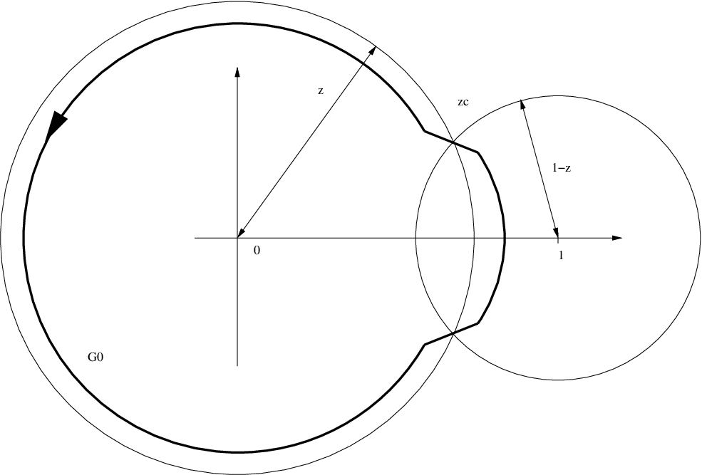
Refer to caption
Figure 6.2: Illustration of the steep descent path.

In this way, we have a steep descent path. Thus,

In,t​(x)=et​Re​(g⁡(wc))​𝒪​(e−μ​t)+2​Re​(12​π​i​∫γlocd​ww​et​g​(w))I_{n,t}(x)=e^{t\mathrm{Re}(g(w_{c}))}\mathcal{O}(e^{-\mu t})+2\mathrm{Re}\left(\frac{1}{2\pi{\rm i}}\int_{\gamma_{\rm loc}}\frac{\mathrm{d}w}{w}e^{tg(w)}\right) (6.32)

with μ∼|g′′​(wc)|​δ2\mu\sim|g^{\prime\prime}(w_{c})|\delta^{2}, as soon as |g′′​(wc)|>0|g^{\prime\prime}(w_{c})|>0, i.e., as soon as the second order term dominates all higher order terms in the Taylor expansion.

The second term of (6.32) is given by

12​π​i​∫γlocd​ww​et​g​(w)\displaystyle\frac{1}{2\pi{\rm i}}\int_{\gamma_{\rm loc}}\frac{\mathrm{d}w}{w}e^{tg(w)} =\displaystyle= 12​π​i​∫−δδd​x​θ^wc​et​g​(wc)​e−12​t​|g′′​(wc)|​x2​e𝒪⁡(t​x3)​𝒪​(x)\displaystyle\frac{1}{2\pi{\rm i}}\int_{-\delta}^{\delta}\mathrm{d}x\frac{\hat{\theta}}{w_{c}}e^{tg(w_{c})}e^{-\tfrac{1}{2}t|g^{\prime\prime}(w_{c})|x^{2}}e^{\mathcal{O}(tx^{3})}\mathcal{O}(x) (6.33)
=\displaystyle= 12​π​i​θ^wc​∫−δδd​x​et​g​(wc)​e−12​t​|g′′​(wc)|​x2+E1\displaystyle\frac{1}{2\pi{\rm i}}\frac{\hat{\theta}}{w_{c}}\int_{-\delta}^{\delta}\mathrm{d}xe^{tg(w_{c})}e^{-\tfrac{1}{2}t|g^{\prime\prime}(w_{c})|x^{2}}+E_{1}

where

E1=12​π​i​θ^wc​∫−δδd​x​et​g​(wc)​e−12​t​|g′′​(wc)|​x2​e𝒪⁡(t​x3)​𝒪​(t​x3,x).E_{1}=\frac{1}{2\pi{\rm i}}\frac{\hat{\theta}}{w_{c}}\int_{-\delta}^{\delta}\mathrm{d}xe^{tg(w_{c})}e^{-\tfrac{1}{2}t|g^{\prime\prime}(w_{c})|x^{2}}e^{\mathcal{O}(tx^{3})}\mathcal{O}(tx^{3},x). (6.34)

Here we used |ex−1|≤|x|​e|x||e^{x}-1|\leq|x|e^{|x|}. Changing variable y=x​ty=x\sqrt{t}, we get that

|E1|\displaystyle|E_{1}| ≤\displaystyle\leq const​et​Re​(g⁡(wc))​1t​∫−δ​tδ​td​y​e−|g′′​(wc)|y2/2​𝒪​(y,y3/t)​e𝒪⁡(y3/t)\displaystyle\mathrm{const\,}e^{t\mathrm{Re}(g(w_{c}))}\frac{1}{t}\int_{-\delta\sqrt{t}}^{\delta\sqrt{t}}\mathrm{d}ye^{-|g^{\prime\prime}(w_{c})|y^{2}/2}\mathcal{O}(y,y^{3}/\sqrt{t})e^{\mathcal{O}(y^{3}/\sqrt{t})} (6.35)
≤\displaystyle\leq const​et​Re​(g⁡(wc))t​|g′′​(wc)|\displaystyle\mathrm{const\,}\frac{e^{t\mathrm{Re}(g(w_{c}))}}{t\sqrt{|g^{\prime\prime}(w_{c})|}}

for δ\delta small enough, i.e., for 0<δ≪|g′′​(wc)|0<\delta\ll|g^{\prime\prime}(w_{c})|. In this small neighborhood, the quadratic term controls the higher order ones. The final step is to extend the integral on the rest of r.h.s. of (6.33) from ±δ\pm\delta to ±∞\pm\infty. This can be made up to an error et​Re​(g⁡(wc))​𝒪​(e−μ​t)e^{t\mathrm{Re}(g(w_{c}))}\mathcal{O}(e^{-\mu t}) as above.

Resuming we have (counting the contribution from both critical points)

In,t\displaystyle I_{n,t} =\displaystyle= et​Re​(g⁡(wc))[𝒪(e−μ​t)+𝒪(1/(t|g′′​(wc)|)]\displaystyle e^{t\mathrm{Re}(g(w_{c}))}\left[\mathcal{O}(e^{-\mu t})+\mathcal{O}(1/(t\sqrt{|g^{\prime\prime}(w_{c})|})\right] (6.36)
+2​R​e​(12​π​i​θ^wc​∫ℝd​x​et​g​(wc)​e−12​t​|g′′​(wc)|​x2).\displaystyle+2\mathrm{Re}\left(\frac{1}{2\pi{\rm i}}\frac{\hat{\theta}}{w_{c}}\int_{\mathbb{R}}\mathrm{d}xe^{tg(w_{c})}e^{-\tfrac{1}{2}t|g^{\prime\prime}(w_{c})|x^{2}}\right).

The error terms are the one indicated in (6.26), and the Gaussian integral for the last term gives

2​et​Re​(g⁡(wc))2​π​t​|wc|2​|g′′​(wc)|​Re​(−i​θ^​|wc|wc​ei​t​Im​(g⁡(wc))).\frac{2e^{t\mathrm{Re}(g(w_{c}))}}{\sqrt{2\pi t\,|w_{c}|^{2}\,|g^{\prime\prime}(w_{c})|}}\mathrm{Re}\left(-{\rm i}\hat{\theta}\frac{|w_{c}|}{w_{c}}e^{{\rm i}t\mathrm{Im}(g(w_{c}))}\right). (6.37)

We then set β=arg(−iθ^/wc)=−π/4−(πc+πλ)/2\beta=\arg(-{\rm i}\hat{\theta}/w_{c})=-\pi/4-(\pi_{c}+\pi_{\lambda})/2, so that −i​θ^​|wc|wc=ei​β-{\rm i}\hat{\theta}\frac{|w_{c}|}{w_{c}}=e^{{\rm i}\beta}. For λ\lambda in a compact subset of ((1−c)2,(1+c)2)((1-\sqrt{c})^{2},(1+\sqrt{c})^{2}), |g′′​(wc)||g^{\prime\prime}(w_{c})| is uniformly bounded away from zero and infinity. Thus the Lemma is proven. ∎

The bound of Lemma 6.4 can be easily extended until position away of order 𝒪⁡(t2/3)\mathcal{O}(t^{2/3}) from the upper edge.

Lemma 6.6.

Set α=Im⁡(g⁡(wc))\alpha=\mathrm{Im}(g(w_{c})) and β=−12​(πc+πλ+π/2)\beta=-\tfrac{1}{2}(\pi_{c}+\pi_{\lambda}+\pi/2). Then, for λ∈[(1−c)2+ε0,(1+c)2−t−1/3]\lambda\in[(1-\sqrt{c})^{2}+\varepsilon_{0},(1+\sqrt{c})^{2}-t^{-1/3}], for any fixed ε0>0\varepsilon_{0}>0, we have the uniform estimate

Ic​t,t(λt)=et​Re​(g⁡(wc))|g′′​(wc)|​t[2π​|wc|2cos(tα+β)+𝒪(t−1/2)+𝒪(te−const​t1/3)].I_{ct,t}(\lambda t)=\frac{e^{t\mathrm{Re}(g(w_{c}))}}{\sqrt{|g^{\prime\prime}(w_{c})|t}}\Bigg[\sqrt{\frac{2}{\pi|w_{c}|^{2}}}\cos(t\alpha+\beta)+\mathcal{O}(t^{-1/2})+\mathcal{O}\Big(\sqrt{t}e^{-\mathrm{const\,}t^{1/3}}\Big)\Bigg]. (6.38)

Proof of Lemma 6.6. The analysis of Lemma 6.4 can be made also for this case, with only minor differences. Indeed, for (1+c)2−λ∼t−1/3(1+\sqrt{c})^{2}-\lambda\sim t^{-1/3}, we have |g′′(wc)|∼t−1/6|g^{\prime\prime}(w_{c})|\sim t^{-1/6} and this time we choose δ\delta going to zero as t→∞t\to\infty, setting δ=t−1/4\delta=t^{-1/4}. With this choice, (6.32) and (6.35) are still valid because at the border of integration the quadratic term dominates the cubic one. Indeed, with y=δ​t=t1/4y=\delta\sqrt{t}=t^{1/4}, it holds y3/t∼t1/4≪t1/3∼|g′′​(wc)|​y2y^{3}/\sqrt{t}\sim t^{1/4}\ll t^{1/3}\sim|g^{\prime\prime}(w_{c})|y^{2}. Also, the error term coming from steep descent in (6.32) will vanish as t→∞t\to\infty but slower than before, with μ​t∼t1/3\mu t\sim t^{1/3}. ∎

The results of Lemma 6.4 and Lemma 6.6 imply the following asymptotics for the functions qnq_{n}’s.

Lemma 6.7.

Set α=Im⁡(g⁡(wc))\alpha=\mathrm{Im}(g(w_{c})) and β=−12​(πc+πλ+π/2)\beta=-\tfrac{1}{2}(\pi_{c}+\pi_{\lambda}+\pi/2) and fix any ε0>0\varepsilon_{0}>0. Then, uniformly in λ∈[(1−c)2+ε0,(1+c)2−t−1/3]\lambda\in[(1-\sqrt{c})^{2}+\varepsilon_{0},(1+\sqrt{c})^{2}-t^{-1/3}], we have

qc​t(λt,t)=1πt−1/2c−(1+c−λ)244[cos(tα+β)+𝒪(t−1/2)].q_{ct}(\lambda t,t)=\frac{1}{\sqrt{\pi}}\frac{t^{-1/2}}{\sqrt[4]{c-\frac{(1+c-\lambda)^{2}}{4}}}\Bigg[\cos(t\alpha+\beta)+\mathcal{O}(t^{-1/2})\Bigg]. (6.39)

Proof of Lemma 6.7. We just have to compute the prefactor Bc​t,t​(λ​t)​et​Re​(g⁡(wc))B_{ct,t}(\lambda t)e^{t\mathrm{Re}(g(w_{c}))}. We have (6.25) and applying Stirling formula for the factorials in Bc​t,t​(λ​t)B_{ct,t}(\lambda t) we get that

Bc​t,t​(λ​t)​et​Re​(g⁡(wc))=(λ/c)1/4​(1+𝒪⁡(1/t)).B_{ct,t}(\lambda t)e^{t\mathrm{Re}(g(w_{c}))}=(\lambda/c)^{1/4}(1+\mathcal{O}(1/t)). (6.40)

∎

Now we need to fill the gap between the bulk and the edge. In this region we do not need precise asymptotics, just a bound. Approaching the upper edge, g′′​(wc)g^{\prime\prime}(w_{c}) goes to zero, but then everything can be controlled by the cubic term, because |g′′′​(wc)|≠0|g^{\prime\prime\prime}(w_{c})|\neq 0 at the edges.

Lemma 6.8.

For ε0>0\varepsilon_{0}>0 fixed but small enough, and ℓ>0\ell>0 large enough, we have the bound

|qc​t​(λ​t,t)|≤const​t−1/2c−(1+c−λ)244,\left|q_{ct}(\lambda t,t)\right|\leq\mathrm{const\,}\frac{t^{-1/2}}{\sqrt[4]{c-\frac{(1+c-\lambda)^{2}}{4}}}, (6.41)

uniformly for λ∈[(1+c)2−ε0,(1+c)2−ℓt−2/3]\lambda\in[(1+\sqrt{c})^{2}-\varepsilon_{0},(1+\sqrt{c})^{2}-\ell t^{-2/3}].

Proof of Lemma 6.8. Consider the ε0\varepsilon_{0}-region close to the upper edge with ε0>0\varepsilon_{0}>0 small enough. We can compute explicitly the direction θ^\hat{\theta}, see (6.31). It is a continuous function of λ\lambda and, as λ↑(1+c)2\lambda\uparrow(1+\sqrt{c})^{2}, θ^↑ei5​π/4\hat{\theta}\uparrow e^{{\rm i}5\pi/4} (because πλ↑π\pi_{\lambda}\uparrow\pi and πc↓0\pi_{c}\downarrow 0). We need just a bound, so we choose θ^=ei5​π/4\hat{\theta}=e^{{\rm i}5\pi/4} and set the local path as

γloc\displaystyle\gamma_{\rm loc} =\displaystyle= {w=wc+ei5​π/4​x,x∈[−δ,Im⁡(wc)​2]}.\displaystyle\{w=w_{c}+e^{{\rm i}5\pi/4}x,x\in[-\delta,\mathrm{Im}(w_{c})\sqrt{2}]\}. (6.42)

The path γloc\gamma_{\rm loc} reaches at x=Im⁡(wc)​2x=\mathrm{Im}(w_{c})\sqrt{2} the imaginary axis and this is the reason for the upper edge of γloc\gamma_{\rm loc}. We have

g⁡(w)=g⁡(wc)+12​g′′​(wc)​(w−wc)2+16​g′′′​(wc)​(w−wc)3+𝒪⁡((w−wc)4).g(w)=g(w_{c})+\tfrac{1}{2}g^{\prime\prime}(w_{c})(w-w_{c})^{2}+\tfrac{1}{6}g^{\prime\prime\prime}(w_{c})(w-w_{c})^{3}+\mathcal{O}((w-w_{c})^{4}). (6.43)

In a δ\delta-neighborhood of wcw_{c}, along the direction θ^\hat{\theta} chosen,

Re⁡(12​g′′​(wc)​(w−wc)2)=−12​|g′′​(wc)|​x2​(1+𝒪⁡(ϵ0))\mathrm{Re}(\tfrac{1}{2}g^{\prime\prime}(w_{c})(w-w_{c})^{2})=-\tfrac{1}{2}|g^{\prime\prime}(w_{c})|x^{2}(1+\mathcal{O}(\epsilon_{0})) (6.44)

and

Re⁡(16​g′′′​(wc)​(w−wc)3)=16​|g′′′​(wc)|​x3/2​(1+𝒪⁡(ϵ0)).\mathrm{Re}(\tfrac{1}{6}g^{\prime\prime\prime}(w_{c})(w-w_{c})^{3})=\tfrac{1}{6}|g^{\prime\prime\prime}(w_{c})|x^{3}/\sqrt{2}(1+\mathcal{O}(\sqrt{\epsilon_{0}})). (6.45)

Therefore, for ε0\varepsilon_{0} small enough, the quadratic term helps the convergence. For x≤0x\leq 0, the cubic term helps the convergence, while for x∈[0,Im⁡(wc)​2]x\in[0,\mathrm{Im}(w_{c})\sqrt{2}] we will need to control it by the quadratic term. Thus,

In,t​(x)=et​Re​(g⁡(wc))​𝒪​(e−μ​t)+2​Re​(12​π​i​∫γlocd​ww​et​g​(w)),I_{n,t}(x)=e^{t\mathrm{Re}(g(w_{c}))}\mathcal{O}(e^{-\mu t})+2\mathrm{Re}\left(\frac{1}{2\pi{\rm i}}\int_{\gamma_{\rm loc}}\frac{\mathrm{d}w}{w}e^{tg(w)}\right), (6.46)

with μ≃|g′′′​(wc)|​δ3\mu\simeq|g^{\prime\prime\prime}(w_{c})|\delta^{3}, where g′′′​(wc)→2/c​(1+c)g^{\prime\prime\prime}(w_{c})\to 2/\sqrt{c}(1+\sqrt{c}) as λ→(1+c)2\lambda\to(1+\sqrt{c})^{2}.

Consider then the contribution coming from the integral over γloc\gamma_{\rm loc}. We have

|∫γlocd​ww​et​g​(w)|\displaystyle\left|\int_{\gamma_{\rm loc}}\frac{\mathrm{d}w}{w}e^{tg(w)}\right| ≤\displaystyle\leq et​Re​(g⁡(wc))|wc|​∫−δIm⁡(wc)​2d​x​exp⁡(−12​t​|g′′​(wc)|​x2)\displaystyle\frac{e^{t\mathrm{Re}(g(w_{c}))}}{|w_{c}|}\int_{-\delta}^{\mathrm{Im}(w_{c})\sqrt{2}}\mathrm{d}x\exp\left(-\tfrac{1}{2}t|g^{\prime\prime}(w_{c})|x^{2}\right) (6.47)
×exp⁡(16​t​|g′′′​(wc)|​x3/2+𝒪⁡(x4​t))​(1+𝒪⁡(x)),\displaystyle\times\exp\left(\tfrac{1}{6}t|g^{\prime\prime\prime}(w_{c})|x^{3}/\sqrt{2}+\mathcal{O}(x^{4}t)\right)(1+\mathcal{O}(x)),

the last 1/21/\sqrt{2} coming from Re(e−iπ/4)=1/2\mathrm{Re}(e^{-{\rm i}\pi/4})=1/\sqrt{2}. A simple verification gives

−12​t​|g′′​(wc)|​x2+16​t|g′′′​(wc)|x3/2≤−14​t|g′′​(wc)|x2,0≤x≤Im⁡(wc)​2.-\tfrac{1}{2}t|g^{\prime\prime}(w_{c})|x^{2}+\tfrac{1}{6}t|g^{\prime\prime\prime}(w_{c})|x^{3}/\sqrt{2}\leq-\tfrac{1}{4}t|g^{\prime\prime}(w_{c})|x^{2},\quad 0\leq x\leq\mathrm{Im}(w_{c})\sqrt{2}. (6.48)

So, for x∈[0,Im⁡(wc)​2]x\in[0,\mathrm{Im}(w_{c})\sqrt{2}], the quadratic term is still dominating higher order terms, including the cubic one (the quartic term can be bounded by replacing 14\tfrac{1}{4} by 16\tfrac{1}{6} in the above estimate).

On the other hand, for −δ≤x≤0-\delta\leq x\leq 0, we have that the cubic term is negative and dominates all higher order terms. More precisely, for δ\delta small enough,

|exp⁡(16​t​|g′′′​(wc)|​x3/2+𝒪⁡(x4​t))|≤exp⁡(112​t​|g′′′​(wc)|​x3)≤1,\left|\exp\left(\tfrac{1}{6}t|g^{\prime\prime\prime}(w_{c})|x^{3}/\sqrt{2}+\mathcal{O}(x^{4}t)\right)\right|\leq\exp\left(\tfrac{1}{12}t|g^{\prime\prime\prime}(w_{c})|x^{3}\right)\leq 1, (6.49)

in the region x∈[−δ,0]x\in[-\delta,0].

Using (6.48) for positive xx and (6.49) for negative xx, we get

(6.47)≤const​et​Re​(g⁡(wc))​∫−δIm⁡(wc)​2d​x​exp⁡(−16​t​|g′′​(wc)|​x2)≤const​et​Re​(g⁡(wc))​1|g′′​(wc)|​t.(\ref{eq6.47})\leq\mathrm{const\,}e^{t\mathrm{Re}(g(w_{c}))}\int_{-\delta}^{\mathrm{Im}(w_{c})\sqrt{2}}\mathrm{d}x\exp\left(-\tfrac{1}{6}t|g^{\prime\prime}(w_{c})|x^{2}\right)\\ \leq\mathrm{const\,}e^{t\mathrm{Re}(g(w_{c}))}\frac{1}{\sqrt{|g^{\prime\prime}(w_{c})|t}}. (6.50)

Replacing the value of |g′′​(wc)||g^{\prime\prime}(w_{c})| into this expression ends the proof. ∎

6.3 Asymptotic of the kernel

In this section we obtain the precise asymptotics of the extended kernel in the bulk first and a bound to control the behavior starting from the upper edge. Here we use several notations introduced in the Section 3.

As usual, it is convenient to conjugate the kernel before taking the limit. For the upper edge (cf. Lemma 6.2) set

Wi,u=exp⁡(−ni​ti+xi​ln⁡(1+ni/ti)−ni​ln⁡(−ni/ti)−ti),W_{i,u}=\exp\left(-\sqrt{n_{i}t_{i}}+x_{i}\ln(1+\sqrt{n_{i}/t_{i}})-n_{i}\ln(-\sqrt{n_{i}/t_{i}})-t_{i}\right), (6.51)

and, in the bulk (see Lemma 6.4) set

Wi,b=exp⁡(12​(ti+ni−xi)−12​ni​ln⁡(ni/ti)+12​xi​ln⁡(xi/ti)−ti).W_{i,b}=\exp\left(\tfrac{1}{2}(t_{i}+n_{i}-x_{i})-\tfrac{1}{2}n_{i}\ln(n_{i}/t_{i})+\tfrac{1}{2}x_{i}\ln(x_{i}/t_{i})-t_{i}\right). (6.52)

Then, define the conjugation as

Wi={Wi,b,for ​(ti−ni)2≤xi≤(ti+ni)2,Wi,u,for ​xi≥(ti+ni)2.W_{i}=\left\{\begin{array}[]{ll}W_{i,b},&\textrm{for }(\sqrt{t_{i}}-\sqrt{n_{i}})^{2}\leq x_{i}\leq(\sqrt{t_{i}}+\sqrt{n_{i}})^{2},\\ W_{i,u},&\textrm{for }x_{i}\geq(\sqrt{t_{i}}+\sqrt{n_{i}})^{2}.\end{array}\right. (6.53)

Remark that WiW_{i} is continuous. Moreover, |Wi,u−Wi,b|=𝒪(L−1/3)|W_{i,u}-W_{i,b}|=\mathcal{O}(L^{-1/3}) for |xi−(ti+ni)2|=𝒪(L−1/3)|x_{i}-(\sqrt{t_{i}}+\sqrt{n_{i}})^{2}|=\mathcal{O}(L^{-1/3}). Therefore in such a neighborhood it is actually irrelevant which formula to use.

Proposition 6.9.

Let us consider two triples (x1,n1,t1)(x_{1},n_{1},t_{1}) and (x2,n2,t2)(x_{2},n_{2},t_{2}) parameterized by

xi=[νi​L],ni=[ηi​L],ti=τi​L.\displaystyle x_{i}=[\nu_{i}L],\quad n_{i}=[\eta_{i}L],\quad t_{i}=\tau_{i}L. (6.54)

Assume that they are in the bulk of the system, namely, that exists ε0>0\varepsilon_{0}>0 such that

(τi−ηi)2+ε0≤νi≤(τi+ηi)2−L−1/3.(\sqrt{\tau_{i}}-\sqrt{\eta_{i}})^{2}+\varepsilon_{0}\leq\nu_{i}\leq(\sqrt{\tau_{i}}+\sqrt{\eta_{i}})^{2}-L^{-1/3}. (6.55)

Denote zc=Ω⁡(ν1,η1,τ1)z_{c}=\Omega(\nu_{1},\eta_{1},\tau_{1}), wc=Ω⁡(ν2,η2,τ2)w_{c}=\Omega(\nu_{2},\eta_{2},\tau_{2}), and assume that these points are not too close: |zc−wc|≥L−1/16|z_{c}-w_{c}|\geq L^{-1/16}. Then, the asymptotic expansion

(W1/W2)​K​(x1,n1,t1,x2,n2,t2)=12​π​L​|G′′​(wc)|​|G′′​(zc)|​|1−zc|\displaystyle(W_{1}/W_{2})K(x_{1},n_{1},t_{1};x_{2},n_{2},t_{2})=\frac{1}{2\pi L\sqrt{|G^{\prime\prime}(w_{c})|\,|G^{\prime\prime}(z_{c})|}|1-z_{c}|} (6.56)
×\displaystyle\times [1wc−zcei​L​Im​(G⁡(wc))+i​β2ei​L​Im​(G⁡(zc))+i​β1+1wc−z¯cei​L​Im​(G⁡(wc))+i​β2e−i​L​Im​(G⁡(zc))−i​β1\displaystyle\bigg[\frac{1}{w_{c}-z_{c}}\frac{e^{{\rm i}L\mathrm{Im}(G(w_{c}))+{\rm i}\beta_{2}}}{e^{{\rm i}L\mathrm{Im}(G(z_{c}))+{\rm i}\beta_{1}}}+\frac{1}{w_{c}-\bar{z}_{c}}\frac{e^{{\rm i}L\mathrm{Im}(G(w_{c}))+{\rm i}\beta_{2}}}{e^{-{\rm i}L\mathrm{Im}(G(z_{c}))-{\rm i}\beta_{1}}}
+1w¯c−zce−i​L​Im​(G⁡(wc))−i​β2ei​L​Im​(G⁡(zc))+i​β1+1w¯c−z¯ce−i​L​Im​(G⁡(wc))−i​β2e−i​L​Im​(G⁡(zc))−i​β1+𝒪(L−1/8)]\displaystyle+\frac{1}{\bar{w}_{c}-z_{c}}\frac{e^{-{\rm i}L\mathrm{Im}(G(w_{c}))-{\rm i}\beta_{2}}}{e^{{\rm i}L\mathrm{Im}(G(z_{c}))+{\rm i}\beta_{1}}}+\frac{1}{\bar{w}_{c}-\bar{z}_{c}}\frac{e^{-{\rm i}L\mathrm{Im}(G(w_{c}))-{\rm i}\beta_{2}}}{e^{-{\rm i}L\mathrm{Im}(G(z_{c}))-{\rm i}\beta_{1}}}+\mathcal{O}(L^{-1/8})\bigg]

holds, with the error uniform in LL for L≥L0≫1L\geq L_{0}\gg 1. The phases β1\beta_{1} and β2\beta_{2} are given by

β1=−5​π4−πν12−πη12,β2=3​π4+πν22−πη22.\beta_{1}=-\frac{5\pi}{4}-\frac{\pi_{\nu_{1}}}{2}-\frac{\pi_{\eta_{1}}}{2},\quad\beta_{2}=\frac{3\pi}{4}+\frac{\pi_{\nu_{2}}}{2}-\frac{\pi_{\eta_{2}}}{2}. (6.57)

Proof of Proposition 6.9. The analysis relies on the double integral representation (4.2) of the kernel. The analysis for the cases (n1,t1)⊀(n2,t2)(n_{1},t_{1})\not\prec(n_{2},t_{2}) and (n1,t1)≺(n2,t2)(n_{1},t_{1})\prec(n_{2},t_{2}) are very similar. Let us explain the first case, corresponding to η1>η2\eta_{1}>\eta_{2}, or τ1<τ2\tau_{1}<\tau_{2}, or (η1,τ1)=(η2,τ2)(\eta_{1},\tau_{1})=(\eta_{2},\tau_{2}). The asymptotics employs several ingredients already used in Lemma 6.4 and Lemma 6.6. Thus, we introduce the notations

ci=ηi/τi⇒ni=[ci​ti],λi=νi/τi⇒xi=[λi​ti].c_{i}=\eta_{i}/\tau_{i}\Rightarrow n_{i}=[c_{i}t_{i}],\quad\lambda_{i}=\nu_{i}/\tau_{i}\Rightarrow x_{i}=[\lambda_{i}t_{i}]. (6.58)

The conjugation factor et1−t2e^{t_{1}-t_{2}} in the kernel representation (4.2) will not appear in the following computations, since it appears automatically in the factors W1/W2W_{1}/W_{2}. Thus, we have to analyze

1(2​π​i)2​∮Γ0d​w​∮Γ1d​z​et2​g2​(w)−t1​g1​(z)​1(1−z)​(w−z)\frac{1}{(2\pi{\rm i})^{2}}\oint_{\Gamma_{0}}\mathrm{d}w\oint_{\Gamma_{1}}\mathrm{d}ze^{t_{2}g_{2}(w)-t_{1}g_{1}(z)}\frac{1}{(1-z)(w-z)} (6.59)

with gi​(w)=w+λi​ln⁡(1−w)−ci​ln⁡(w)≡G⁡(w|λi,ci,1)g_{i}(w)=w+\lambda_{i}\ln(1-w)-c_{i}\ln(w)\equiv G(w|\lambda_{i},c_{i},1), i=1,2i=1,2.

The critical points of g2​(w)g_{2}(w) and g1​(z)g_{1}(z) are given by

wc=Ω⁡(λ2,c2,1)=Ω⁡(ν2,η2,τ2),zc=Ω⁡(λ1,c1,1)=Ω⁡(ν1,η1,τ1).w_{c}=\Omega(\lambda_{2},c_{2},1)=\Omega(\nu_{2},\eta_{2},\tau_{2}),\quad z_{c}=\Omega(\lambda_{1},c_{1},1)=\Omega(\nu_{1},\eta_{1},\tau_{1}). (6.60)

The integrals over ww are, up to the factor w/(z−w)w/(z-w), as in Lemma 6.4. Therefore, the steep descent path Γ0\Gamma_{0} is chosen as in Lemma 6.4 and the steep descent path Γ1\Gamma_{1} is chosen in a similar way. We illustrate these paths if the critical point is ζc\zeta_{c}, see Figure 6.3.

Refer to caption
Figure 6.3: Illustration of the steep descent paths.

In particular, |wc|=η2/τ2|w_{c}|=\sqrt{\eta_{2}/\tau_{2}} and |zc|=η1/τ2|z_{c}|=\sqrt{\eta_{1}/\tau_{2}}. In our case, we have |wc|≤|zc||w_{c}|\leq|z_{c}| and |wc−zc|≥L−1/16|w_{c}-z_{c}|\geq L^{-1/16}. The steep descent paths described above actually intersect. Therefore, we have to correct (6.59) by subtracting the residue at z=wz=w, as indicated in Figure 6.4. We call “main term” the contribution of the integral with Γ0\Gamma_{0} and Γ1\Gamma_{1} crossing, while we call “residual term” the contribution of the residue.

Notice that the integral with the paths Γ0\Gamma_{0} and Γ1\Gamma_{1} crossing is integrable in the usual sense, because the divergence term 1/(w−z)1/(w-z) is integrable. The contribution of the main term is the following.

Refer to caption
Figure 6.4: The subdivision of the integration (6.59). We have |zc|≥|wc||z_{c}|\geq|w_{c}| and when |zc|=|wc||z_{c}|=|w_{c}|, they are not at the same position.

Both integrals can be divided as the part in ℍ\mathbbm{H} and its complex conjugate. Therefore, in the final expression we get the sum of four terms. Now, we restrict our attention to the integral over the path Γ0\Gamma_{0} and Γ1\Gamma_{1} on ℍ\mathbbm{H}. The analysis of the integral over Γ0\Gamma_{0} is the same as in Lemma 6.4 except for the missing 1/wc1/w_{c} factor and that instead of 2​Re​(⋯)2\mathrm{Re}(\cdots) we just have (⋯)(\cdots) in (6.36). The integral over Γ1\Gamma_{1} is similar.

This time we choose the cutoff for the evaluation of the term with the steep descent path equal to δ=L−1/4\delta=L^{-1/4}. There are two reasons. The first one is that we want to get the expansion valid also for νi\nu_{i} up to L−1/3L^{-1/3} away from the upper edge, compare with Lemma 6.6. The second reason is that we have the extra factor 1/(w−z)1/(w-z). The contributions of the steep descent path do not create problems, since the factor is integrable in the usual sense (just need a bound). However, with our choice of δ\delta, in the contribution of the δ\delta-neighborhoods of zcz_{c} and wcw_{c} we have

1/(w−z)=1/(wc−zc)+𝒪(δ/|wc−zc|2)=1/(wc−zc)+𝒪(L−1/8),1/(w-z)=1/(w_{c}-z_{c})+\mathcal{O}(\delta/|w_{c}-z_{c}|^{2})=1/(w_{c}-z_{c})+\mathcal{O}(L^{-1/8}), (6.61)

with δ=L−1/4\delta=L^{-1/4} and |wc−zc|≥L−1/16|w_{c}-z_{c}|\geq L^{-1/16}. In the end, the contribution of the main term is given by

1wc−zcet2​Re​(g2​(wc))2​π​t2​|g2′′​(wc)|[et2​Im​(g2​(wc))θ^2(wc)+𝒪(L−1/2)]\displaystyle\frac{1}{w_{c}-z_{c}}\frac{e^{t_{2}\mathrm{Re}(g_{2}(w_{c}))}}{\sqrt{2\pi t_{2}|g_{2}^{\prime\prime}(w_{c})|}}\bigg[e^{t_{2}\mathrm{Im}(g_{2}(w_{c}))}\hat{\theta}_{2}(w_{c})+\mathcal{O}\left(L^{-1/2}\right)\bigg] (6.62)
×\displaystyle\times e−t1​Re​(g1​(zc))2​π​t1​|g1′′​(zc)|ei​πc1|1−zc|[e−t1​Im​(g1​(zc))θ^1(zc)+𝒪(L−1/2)]\displaystyle\frac{e^{-t_{1}\mathrm{Re}(g_{1}(z_{c}))}}{\sqrt{2\pi t_{1}|g_{1}^{\prime\prime}(z_{c})|}}\frac{e^{{\rm i}\pi_{c_{1}}}}{|1-z_{c}|}\bigg[e^{-t_{1}\mathrm{Im}(g_{1}(z_{c}))}\hat{\theta}_{1}(z_{c})+\mathcal{O}\left(L^{-1/2}\right)\bigg]
+\displaystyle+ et2​Re​(g2​(wc))2​π​t2​|g2′′​(wc)|e−t1​Re​(g1​(zc))2​π​t1​|g1′′​(zc)|1|1−zc|𝒪(L−1/8).\displaystyle\frac{e^{t_{2}\mathrm{Re}(g_{2}(w_{c}))}}{\sqrt{2\pi t_{2}|g_{2}^{\prime\prime}(w_{c})|}}\frac{e^{-t_{1}\mathrm{Re}(g_{1}(z_{c}))}}{\sqrt{2\pi t_{1}|g_{1}^{\prime\prime}(z_{c})|}}\frac{1}{|1-z_{c}|}\mathcal{O}(L^{-1/8}).

The term ei​πc1e^{{\rm i}\pi_{c_{1}}} is the phase of 1/(1−zc)1/(1-z_{c}), while θ^i\hat{\theta}_{i} are the directions of the steepest descent paths at the critical points. Explicitly,

θ^1​(zc)\displaystyle\hat{\theta}_{1}(z_{c}) =exp⁡(i⁡(π−12​arg⁡(g′′​(zc))))=exp⁡(i3​π/4+i⁡(πλ1−πc1)/2),\displaystyle=\exp({\rm i}(\pi-\tfrac{1}{2}\arg(g^{\prime\prime}(z_{c}))))=\exp({\rm i}3\pi/4+{\rm i}(\pi_{\lambda_{1}}-\pi_{c_{1}})/2), (6.63)
θ^2​(wc)\displaystyle\hat{\theta}_{2}(w_{c}) =exp⁡(i⁡(π2−12​arg⁡(g′′​(wc))))=exp⁡(i5​π/4+i⁡(πλ2−πc2)/2).\displaystyle=\exp({\rm i}(\tfrac{\pi}{2}-\tfrac{1}{2}\arg(g^{\prime\prime}(w_{c}))))=\exp({\rm i}5\pi/4+{\rm i}(\pi_{\lambda_{2}}-\pi_{c_{2}})/2).

Putting together the four terms (two times two critical points) we get the complete contribution of the main term as

et2​Re​(g2​(wc))−t1​Re​(g1​(zc))2​π​t1​t2​|1−zc|2​|g2′′​(wc)|​|g1′′​(zc)|[𝒪(L−1/8)\displaystyle\frac{e^{t_{2}\mathrm{Re}(g_{2}(w_{c}))-t_{1}\mathrm{Re}(g_{1}(z_{c}))}}{2\pi\sqrt{t_{1}t_{2}|1-z_{c}|^{2}|g_{2}^{\prime\prime}(w_{c})||g_{1}^{\prime\prime}(z_{c})|}}\bigg[\mathcal{O}(L^{-1/8}) (6.64)
+\displaystyle+ 1wc−zc​ei​t2​Im​(g2​(wc))+i​β2ei​t1​Im​(g1​(zc))+i​β1+1wc−z¯c​ei​t2​Im​(g2​(wc))+i​β2e−i​t1​Im​(g1​(zc))−i​β1\displaystyle\frac{1}{w_{c}-z_{c}}\frac{e^{{\rm i}t_{2}\mathrm{Im}(g_{2}(w_{c}))+{\rm i}\beta_{2}}}{e^{{\rm i}t_{1}\mathrm{Im}(g_{1}(z_{c}))+{\rm i}\beta_{1}}}+\frac{1}{w_{c}-\bar{z}_{c}}\frac{e^{{\rm i}t_{2}\mathrm{Im}(g_{2}(w_{c}))+{\rm i}\beta_{2}}}{e^{-{\rm i}t_{1}\mathrm{Im}(g_{1}(z_{c}))-{\rm i}\beta_{1}}}
+\displaystyle+ 1w¯c−zce−i​t2​Im​(g2​(wc))−i​β2ei​t1​Im​(g1​(zc))+i​β1+1w¯c−z¯ce−i​t2​Im​(g2​(wc))−i​β2e−i​t1​Im​(g1​(zc))−i​β1],\displaystyle\frac{1}{\bar{w}_{c}-z_{c}}\frac{e^{-{\rm i}t_{2}\mathrm{Im}(g_{2}(w_{c}))-{\rm i}\beta_{2}}}{e^{{\rm i}t_{1}\mathrm{Im}(g_{1}(z_{c}))+{\rm i}\beta_{1}}}+\frac{1}{\bar{w}_{c}-\bar{z}_{c}}\frac{e^{-{\rm i}t_{2}\mathrm{Im}(g_{2}(w_{c}))-{\rm i}\beta_{2}}}{e^{-{\rm i}t_{1}\mathrm{Im}(g_{1}(z_{c}))-{\rm i}\beta_{1}}}\bigg],

with β1=−arg⁡(θ^1​(zc))−πc1\beta_{1}=-\arg(\hat{\theta}_{1}(z_{c}))-\pi_{c_{1}} and β2=arg⁡(θ^2​(wc))\beta_{2}=\arg(\hat{\theta}_{2}(w_{c})). Finally, we replace gi​(w)​ti=G⁡(w|νi,ηi,τi)​Lg_{i}(w)t_{i}=G(w|\nu_{i},\eta_{i},\tau_{i})L, πλi=πνi\pi_{\lambda_{i}}=\pi_{\nu_{i}}, πci=πνi\pi_{c_{i}}=\pi_{\nu_{i}}, and

et2​Re​(g2​(wc))−t1​Re​(g1​(zc))​et1−t2=W2/W1e^{t_{2}\mathrm{Re}(g_{2}(w_{c}))-t_{1}\mathrm{Re}(g_{1}(z_{c}))}e^{t_{1}-t_{2}}=W_{2}/W_{1} (6.65)

to get (6.56).

The final step is to estimate the contribution of the residual term (the last case of Figure 6.4). It is given by

12​π​i​∫ζζ¯d​z​e(τ2−τ1)​L​z​e(η1−η2)​L​ln⁡(z)(1−z)(ν1−ν2)​L+1,\frac{1}{2\pi{\rm i}}\int_{\zeta}^{\bar{\zeta}}\mathrm{d}z\frac{e^{(\tau_{2}-\tau_{1})Lz}e^{(\eta_{1}-\eta_{2})L\ln(z)}}{(1-z)^{(\nu_{1}-\nu_{2})L+1}}, (6.66)

where ζ\zeta and ζ¯\bar{\zeta} are the two intersection points of the steep descent path Γ0\Gamma_{0} and Γ1\Gamma_{1}. Since τ2−τ1≥0\tau_{2}-\tau_{1}\geq 0, η1−η2≥0\eta_{1}-\eta_{2}\geq 0, and |1−z|=const|1-z|=\mathrm{const\,} along the piece of Γ1\Gamma_{1} inside Γ0\Gamma_{0}, we have Re⁡(z)≤Re⁡(ζ)\mathrm{Re}(z)\leq\mathrm{Re}(\zeta) and Re⁡(ln⁡(z))≤Re⁡(ln⁡(ζ))\mathrm{Re}(\ln(z))\leq\mathrm{Re}(\ln(\zeta)). Therefore,

|(6.66)|≤et2​Re​(g2​(ζ))−t1​Re​(g1​(ζ))≤et2​Re​(g2​(wc))−t1​Re​(g1​(zc))​𝒪​(e−μ1​t1​e−μ2​t2),|(\ref{eq4.41})|\leq e^{t_{2}\mathrm{Re}(g_{2}(\zeta))-t_{1}\mathrm{Re}(g_{1}(\zeta))}\leq e^{t_{2}\mathrm{Re}(g_{2}(w_{c}))-t_{1}\mathrm{Re}(g_{1}(z_{c}))}\mathcal{O}(e^{-\mu_{1}t_{1}}e^{-\mu_{2}t_{2}}), (6.67)

for some positive μ1,μ2\mu_{1},\mu_{2} and at least one larger than L−1/8L^{-1/8}. This follows from the fact that either one (or both) critical points are away of order L−1/16L^{-1/16} from ζ\zeta, and ζ\zeta lies on the steep descent paths of g2​(w)g_{2}(w) and −g1​(z)-g_{1}(z), with local quadratic behavior. ∎

While doing time integration we will also need the following corollary.

Corollary 6.10.

Consider the same setting of Proposition 6.9. Then
(a) the formula for K⁡(x1,n1,t1,x2+1,n2,t2)K(x_{1},n_{1},t_{1};x_{2}+1,n_{2},t_{2}) is the same as (6.56) but with an extra factor (1−wc)(1-w_{c}), resp. (1−w¯c)(1-\bar{w}_{c}), to the terms with ei​β2e^{{\rm i}\beta_{2}}, resp. e−i​β2e^{-{\rm i}\beta_{2}}.
(b) the formula for K⁡(x1,n1−1,t1,x2,n2,t2)K(x_{1},n_{1}-1,t_{1};x_{2},n_{2},t_{2}) is the same as (6.56) but with an extra factor zc−1z_{c}^{-1}, resp. (z¯c)−1(\bar{z}_{c})^{-1}, to the terms with e−i​β1e^{-{\rm i}\beta_{1}}, resp. ei​β1e^{{\rm i}\beta_{1}}.

Proof of Corollary 6.10. The proof is almost identical to the one of Proposition 6.9. The only difference is that in (6.59) we have for (a) an extra term (1−w)(1-w) and for (b) an extra 1/z1/z. ∎

At this point we have all the needed estimates in the bulk. However, since our system develops facets, we need to have control at the upper edge. We will just need some bounds and, since the integrals are the same as in Section 6.1, apart from the factor 1/(wc−zc)1/(w_{c}-z_{c}), which we will assume bounded away from zero.

Proposition 6.11.

Consider the setting of Proposition 6.9, but with one or both of the νi\nu_{i} close to the upper edge,

(τi+ηi)2−L−1/3≤νi≤(τi+ηi)2−ℓL−2/3.(\sqrt{\tau_{i}}+\sqrt{\eta_{i}})^{2}-L^{-1/3}\leq\nu_{i}\leq(\sqrt{\tau_{i}}+\sqrt{\eta_{i}})^{2}-\ell L^{-2/3}. (6.68)

Moreover, assume that |zc−wc||z_{c}-w_{c}| is bounded away from zero uniformly in LL. Then, there exists ℓ\ell large enough, such that

(W1/W2)​|K⁡(x1,n1,t1,x2,n2,t2)|≤constL​∏i=12ηi​τi−14​(τi+ηi−νi)24\displaystyle(W_{1}/W_{2})|K(x_{1},n_{1},t_{1};x_{2},n_{2},t_{2})|\leq\frac{\mathrm{const\,}}{L\prod_{i=1}^{2}\sqrt[4]{\eta_{i}\tau_{i}-\tfrac{1}{4}(\tau_{i}+\eta_{i}-\nu_{i})^{2}}} (6.69)

uniformly in LL for L≥L0≫1L\geq L_{0}\gg 1.

Proof of Proposition 6.11. The proof follows the same argument as Lemma 6.8 for the variables which are close to the edge. For the one which is away from the edges, it is a consequence of the analysis Proposition 6.9. ∎

When one or both positions are at the edge, we need a different bound.

Proposition 6.12.

Consider the setting of Proposition 6.9, but now with ν2\nu_{2} at the edge or in the facet, i.e.,

ν2≥(τ2+η2)2−ℓL−2/3\nu_{2}\geq(\sqrt{\tau_{2}}+\sqrt{\eta_{2}})^{2}-\ell L^{-2/3} (6.70)

for any fixed ℓ\ell. Assume |zc+η2/τ2||z_{c}+\sqrt{\eta_{2}/\tau_{2}}| is bounded away from zero uniformly in LL. Then,

(W1/W2)​|K⁡(x1,n1,t1,x2,n2,t2)|\displaystyle(W_{1}/W_{2})|K(x_{1},n_{1},t_{1};x_{2},n_{2},t_{2})| ≤\displaystyle\leq constL​η1​τ1−14​(τ1+η1−ν1)24\displaystyle\frac{\mathrm{const\,}}{\sqrt{L}\sqrt[4]{\eta_{1}\tau_{1}-\tfrac{1}{4}(\tau_{1}+\eta_{1}-\nu_{1})^{2}}} (6.71)
×\displaystyle\times 1L1/3​exp⁡(−x2−(τ2+η2)2​L(τ2​L)1/3),\displaystyle\frac{1}{L^{1/3}}\exp\left(-\frac{x_{2}-(\sqrt{\tau_{2}}+\sqrt{\eta_{2}})^{2}L}{(\tau_{2}L)^{1/3}}\right),

uniformly in LL for L≥L0≫1L\geq L_{0}\gg 1.

Proof of Proposition 6.12. The proof is obtained along the same lines as Lemmas 6.1 and 6.2. With respect to those cases, the integral has however an extra factor 1/(w−z)1/(w-z). Since we need just a bound, it can simply be replaced by 1/(wc−zc)1/(w_{c}-z_{c}) as follows. In Lemma 6.1 wcw_{c} is replaced by −η2/τ2-\sqrt{\eta_{2}/\tau_{2}}, while in Lemma 6.2, we need to replace wcw_{c} by ρ\rho as given in (6.15). Notice that in the last case we can take |wc+η2/τ2||w_{c}+\sqrt{\eta_{2}/\tau_{2}}| as small as desired. The assumption |zc+η2/τ2|>0|z_{c}+\sqrt{\eta_{2}/\tau_{2}}|>0 uniformly in LL ensures then that 1/(wc−zc)1/(w_{c}-z_{c}) remains bounded as L→∞L\to\infty. ∎

The last case to consider is when both ν1\nu_{1} and ν2\nu_{2} are at the upper edge.

Proposition 6.13.

Consider the setting of Proposition 6.9, but now with ν1\nu_{1} and ν2\nu_{2} at the edge or in the facet, i.e., with

νi≥(τi+ηi)2−ℓL−2/3,i=1,2,\nu_{i}\geq(\sqrt{\tau_{i}}+\sqrt{\eta_{i}})^{2}-\ell L^{-2/3},\quad i=1,2, (6.72)

for any fixed ℓ\ell. Assume that |η2/τ2−η1/τ1||\sqrt{\eta_{2}/\tau_{2}}-\sqrt{\eta_{1}/\tau_{1}}| is bounded away from zero uniformly in LL. Then,

(W1/W2)​|K⁡(x1,n1,t1,x2,n2,t2)|≤const\displaystyle(W_{1}/W_{2})|K(x_{1},n_{1},t_{1};x_{2},n_{2},t_{2})|\leq\mathrm{const\,} (6.73)
1L2/3​exp⁡(−x2−(τ2+η2)2​L(τ2​L)1/3)​exp⁡(−x1−(τ1+η1)2​L(τ1​L)1/3),\displaystyle\frac{1}{L^{2/3}}\exp\left(-\frac{x_{2}-(\sqrt{\tau_{2}}+\sqrt{\eta_{2}})^{2}L}{(\tau_{2}L)^{1/3}}\right)\exp\left(-\frac{x_{1}-(\sqrt{\tau_{1}}+\sqrt{\eta_{1}})^{2}L}{(\tau_{1}L)^{1/3}}\right),

uniformly in LL for L≥L0≫1L\geq L_{0}\gg 1.

Proof of Proposition 6.13. The proof is like Proposition 6.12. We will have |wc+η2/τ2||w_{c}+\sqrt{\eta_{2}/\tau_{2}}| and |zc+η1/τ1||z_{c}+\sqrt{\eta_{1}/\tau_{1}}| as small as desired. The assumption |η2/τ2−η1/τ1|>0|\sqrt{\eta_{2}/\tau_{2}}-\sqrt{\eta_{1}/\tau_{1}}|>0 uniformly in LL allows us to easily bound uniformly in LL the term 1/(wc−zc)1/(w_{c}-z_{c}). ∎

Appendix A Determinantal structure of the correlation functions

Let 𝔛1,…,𝔛N\mathfrak{X}_{1},\dots,\mathfrak{X}_{N} be finite sets and c⁡(1),…,c⁡(N)c(1),\dots,c(N) be arbitrary nonnegative integers. Consider the set

𝔛=(𝔛1⊔⋯⊔𝔛1)⊔⋯⊔(𝔛N⊔⋯⊔𝔛N)\mathfrak{X}=(\mathfrak{X}_{1}\sqcup\dots\sqcup\mathfrak{X}_{1})\sqcup\dots\sqcup(\mathfrak{X}_{N}\sqcup\dots\sqcup\mathfrak{X}_{N}) (A.1)

with c⁡(n)+1c(n)+1 copies of each 𝔛n\mathfrak{X}_{n}. We want to consider a particular form of weight W⁡(X)W(X) for any subset X⊂𝔛X\subset\mathfrak{X}, which turns out to have determinantal correlations.

To define the weight we need a bit of notations. Let

ϕn​(⋅,⋅):𝔛n−1×𝔛n→ℂ,\displaystyle\phi_{n}(\,\cdot\,,\,\cdot\,):\mathfrak{X}_{n-1}\times\mathfrak{X}_{n}\to\mathbb{C}, n=2,…,N,\displaystyle n=2,\dots,N, (A.2)
ϕn​(virt,⋅):𝔛n→ℂ,\displaystyle\phi_{n}(\virt,\,\cdot\,):\mathfrak{X}_{n}\to\mathbb{C}, n=1,…,N,\displaystyle n=1,\dots,N,
ΨjN​(⋅):𝔛N→ℂ,\displaystyle\Psi^{N}_{j}(\,\cdot\,):\mathfrak{X}_{N}\to\mathbb{C}, j=0,…,N−1,\displaystyle j=0,\dots,N-1,

be arbitrary functions on the corresponding sets. Here the symbol virt\virt stands for a “virtual” variable, which is convenient to introduce for notational purposes. In applications virt\virt can sometimes be replaced by +∞+\infty or −∞-\infty. The ϕn\phi_{n} represents the transitions from 𝔛n−1\mathfrak{X}_{n-1} to 𝔛n\mathfrak{X}_{n}.

Also, let

t0N≤⋯≤tc⁡(N)N=t0N−1≤⋯≤tc⁡(N−1)N−1=t0N−2≤⋯≤tc⁡(2)2=t01≤⋯≤tc⁡(1)1t_{0}^{N}\leq\dots\leq t_{c(N)}^{N}=t_{0}^{N-1}\leq\dots\leq t_{c(N-1)}^{N-1}=t_{0}^{N-2}\leq\dots\leq t^{2}_{c(2)}=t^{1}_{0}\leq\dots\leq t^{1}_{c(1)} (A.3)

be real numbers. In applications, these numbers refer to time moments. Finally, let

𝒯tan,ta−1n(⋅,⋅):𝔛n×𝔛n→ℂ,n=1,…,N,a=1,…,c(n),{\cal T}_{t_{a}^{n},t_{a-1}^{n}}(\,\cdot\,,\,\cdot\,):\mathfrak{X}_{n}\times\mathfrak{X}_{n}\to\mathbb{C},\qquad n=1,\dots,N,\quad a=1,\dots,c(n), (A.4)

be arbitrary functions. The 𝒯tan,ta−1n{\cal T}_{t_{a}^{n},t_{a-1}^{n}} represents the transition between two copies of 𝔛n\mathfrak{X}_{n} associated to “times” ta−1nt^{n}_{a-1} and tant^{n}_{a}.

Then, to any subset X⊂𝔛X\subset\mathfrak{X} assign its weight W⁡(X)W(X) as follows. W⁡(X)W(X) is zero unless XX has exactly nn points in each copy of 𝔛n\mathfrak{X}_{n}, n=1,…,Nn=1,\dots,N. In the latter case, denote the points of XX in the mmth copy of 𝔛n\mathfrak{X}_{n} by xkn​(tmn)x^{n}_{k}(t^{n}_{m}), k=1,…,nk=1,\dots,n, m=0,…,c⁡(n)m=0,\ldots,c(n). Thus,

X={xkn(tmn)|k=1,…,n;m=0,…,c(n);n=1,…,N}.X=\{x^{n}_{k}(t^{n}_{m})\,|\,k=1,\dots,n;\,m=0,\dots,c(n);\,n=1,\dots,N\}. (A.5)

Set

W⁡(X)=\displaystyle W(X)= ∏n=1N[det[ϕn(xkn−1(t0n−1),xln(tnc⁡(n)))]1≤k,l≤n\displaystyle\prod_{n=1}^{N}\Bigg[\det{\bigl[\phi_{n}(x_{k}^{n-1}(t_{0}^{n-1}),x_{l}^{n}(t^{n}_{c(n)}))\bigr]}_{1\leq k,l\leq n} (A.6)
×∏a=1c⁡(n)det[𝒯tan,ta−1n(xkn(tna),xnl(tna−1))]1≤k,l≤n]det[ΨNN−l(xNk(t0N))]1≤k,l≤N,\displaystyle\times\prod_{a=1}^{c(n)}\det{\bigl[{\cal T}_{t_{a}^{n},t_{a-1}^{n}}(x_{k}^{n}(t^{n}_{a}),x^{n}_{l}(t^{n}_{a-1}))\bigr]}_{1\leq k,l\leq n}\Bigg]\det{\bigl[\Psi^{N}_{N-l}(x^{N}_{k}(t_{0}^{N}))\bigr]}_{1\leq k,l\leq N},

where xnn−1​(⋅)=virtx^{n-1}_{n}(\,\cdot\,)=\virt for all n=1,…,Nn=1,\dots,N.

In what follows we assume that the partition function of our weights does not vanish:

Z:=∑X⊂𝔛W⁡(X)≠0.Z:=\sum_{X\subset\mathfrak{X}}W(X)\neq 0. (A.7)

Under this assumption, the normalized weights W~​(X)=W​(X)/Z\widetilde{W}(X)=W(X)/Z define a (generally speaking, complex valued) measure on 2𝔛2^{\mathfrak{X}} of total mass 11. One can say that we have a (complex valued) random point process on 𝔛\mathfrak{X}, and its correlation functions are defined accordingly, see e.g. [15]. We are interested in computing these correlation functions.

Let us introduce the compact notation for the convolution of several transitions. For any n=1,…,Nn=1,\dots,N and two time moments tan>tbnt_{a}^{n}>t_{b}^{n} we define

𝒯tan,tbn=𝒯tan,ta−1n∗𝒯ta−1n,ta−2n∗⋯∗𝒯tb+1n,tbn,𝒯n=𝒯tc⁡(n)n,t0n,{\cal T}_{t_{a}^{n},t_{b}^{n}}={\cal T}_{t_{a}^{n},t_{a-1}^{n}}*{\cal T}_{t_{a-1}^{n},t_{a-2}^{n}}*\cdots*{\cal T}_{t_{b+1}^{n},t_{b}^{n}},\qquad{{\cal T}}^{n}={{\cal T}}_{t_{c(n)}^{n},t_{0}^{n}}, (A.8)

where we use the notation (f∗g)​(x,y):=∑zf⁡(x,z)​g​(z,y).(f*g)(x,y):=\sum_{z}f(x,z)g(z,y). For any time moments ta1n1≥ta2n2t_{a_{1}}^{n_{1}}\geq t_{a_{2}}^{n_{2}} with (a1,n1)≠(a2,n2)(a_{1},n_{1})\neq(a_{2},n_{2}), we denote the convolution over all the transitions between them by ϕ(ta1n1,ta2n2)\phi^{(t_{a_{1}}^{n_{1}},t_{a_{2}}^{n_{2}})}:

ϕ(ta1n1,ta2n2)=𝒯ta1n1,t0n1∗ϕn1+1∗𝒯n1+1∗⋯∗ϕn2∗𝒯tc⁡(n2)n2,ta2n2.\phi^{(t_{a_{1}}^{n_{1}},t_{a_{2}}^{n_{2}})}={{\cal T}}_{t^{n_{1}}_{a_{1}},t^{n_{1}}_{0}}*\,\phi_{n_{1}+1}*{{\cal T}}^{n_{1}+1}*\cdots*\phi_{n_{2}}*{{\cal T}}_{t^{n_{2}}_{c(n_{2})},t^{n_{2}}_{a_{2}}}. (A.9)

If there are no such transitions, i.e., if ta1n1<ta2n2t_{a_{1}}^{n_{1}}<t_{a_{2}}^{n_{2}} or (a1,n1)=(a2,n2)(a_{1},n_{1})=(a_{2},n_{2}), we set ϕ(ta1n1,ta2n2)=0\phi^{(t_{a_{1}}^{n_{1}},t_{a_{2}}^{n_{2}})}=0.

Furthermore, define the matrix M=‖Mk,l‖k,l=1NM={\|M_{k,l}\|}_{k,l=1}^{N} by

Mk,l=(ϕk∗𝒯k∗⋯∗ϕN∗𝒯N∗ΨN−lN)(virt)M_{k,l}=\big(\phi_{k}*{{\cal T}}^{k}*\cdots*\phi_{N}*{{\cal T}}^{N}*\Psi^{N}_{N-l}\big)(\virt) (A.10)

and the vector

Ψn,tann−l=ϕ(tan,t0N)∗ΨNN−l,l=1,…,N.\Psi^{n,t^{n}_{a}}_{n-l}=\phi^{(t^{n}_{a},t^{N}_{0})}*\Psi^{N}_{N-l},\qquad l=1,\dots,N. (A.11)

The following statement describing the correlation kernel is a part of Theorem 4.2 of [7].

Theorem A.1.

Assume that the matrix MM is invertible. Then Z=detM≠0Z=\det M\neq 0, and the (complex valued) random point process on 𝔛\mathfrak{X} defined by the weights W~​(X)\widetilde{W}(X) is determinantal. Its correlation kernel can be written in the form

K⁡(ta1n1,x1,ta2n2,x2)\displaystyle K(t^{n_{1}}_{a_{1}},x_{1};t^{n_{2}}_{a_{2}},x_{2}) =−ϕ(ta1n1,ta2n2)​(x1,x2)\displaystyle=-\phi^{(t^{n_{1}}_{a_{1}},t^{n_{2}}_{a_{2}})}(x_{1},x_{2}) (A.12)
+\displaystyle+ ∑k=1N∑l=1n2Ψn1−kn1,ta1n1​(x1)​[M−1]k,l​(ϕl∗ϕ(tc⁡(l)l,ta2n2))​(virt,x2).\displaystyle\sum_{k=1}^{N}\sum_{l=1}^{n_{2}}\Psi^{n_{1},t^{n_{1}}_{a_{1}}}_{n_{1}-k}(x_{1})[M^{-1}]_{k,l}(\phi_{l}*\phi^{(t^{l}_{c(l)},t^{n_{2}}_{a_{2}})})(\virt,x_{2}).

The proof of Theorem A.1 given in [7] is based on the algebraic formalism of [15]. Another proof can be found in Section 4.4 of [26]. Although we stated Theorem A.1 for the case when all sets 𝔛n\mathfrak{X}_{n} are finite, one easily extends it to a more general setting. Indeed, the determinantal formula for the correlation functions is an algebraic identity, and the limit transition to the case when 𝔛n\mathfrak{X}_{n}’s are allowed to be countably infinite is immediate, under the assumption that all the sums needed to define the ∗*-operations above are absolutely convergent. Another easy extension (which we do not need in this paper) is the case when the spaces 𝔛j\mathfrak{X}_{j} become continuous, and the sums have to be replaced by the corresponding integrals over these spaces.

References

  • [1] M. Balázs and J. Komjáthy, Order of current variance and diffusivity in the rate one totally asymmetric zero range process, J. Stat. Phys. 133 (2008), 59–78.
  • [2] M. Balázs and T. Seppäläinen, Order of current variance and diffusivity in the asymmetric simple exclusion process, arXiv:math.PR/0608400 (2006).
  • [3] A.L. Barabási and H.E. Stanley, Fractal concepts in surface growth, Cambridge University Press, Cambridge, 1995.
  • [4] H. van Beijeren, R. Kutner, and H. Spohn, Excess noise for driven diffusive systems, Phys. Rev. Lett. 54 (1985), 2026–2029.
  • [5] P. Biane, Approximate factorization and concentration for characters of symmetric groups, Int. Math. Res. Not. 4 (2001), 179–192.
  • [6] A. Borodin, Loop-free markov chains as determinantal point processes, Ann. de l’Institut Henri Poincaré - Prob. et Stat. 44 (2008), 19–28.
  • [7] A. Borodin and P.L. Ferrari, Large time asymptotics of growth models on space-like paths I: PushASEP, Electron. J. Probab. 13 (2008), 1380––1418.
  • [8] A. Borodin, P.L. Ferrari, and M. Prähofer, Fluctuations in the discrete TASEP with periodic initial configurations and the Airy1 process, Int. Math. Res. Papers 2007 (2007), rpm002.
  • [9] A. Borodin, P.L. Ferrari, M. Prähofer, and T. Sasamoto, Fluctuation properties of the TASEP with periodic initial configuration, J. Stat. Phys. 129 (2007), 1055–1080.
  • [10] A. Borodin, P.L. Ferrari, and T. Sasamoto, Large time asymptotics of growth models on space-like paths II: PNG and parallel TASEP, Comm. Math. Phys. 283 (2008), 417–449.
  • [11] A. Borodin, P.L. Ferrari, and T. Sasamoto, Transition between Airy1 and Airy2 processes and TASEP fluctuations, Comm. Pure Appl. Math. 61 (2008), 1603–1629.
  • [12] A. Borodin and V. Gorin, Shuffling algorithm for boxed plane partitions, preprint: arXiv:0804.3071 (2008).
  • [13] A. Borodin and J. Kuan, Asymptotics of Plancherel measures for the infinite-dimensional unitary group, Adv. Math. 219 (2008), 894–931.
  • [14] A. Borodin, A. Okounkov, and G. Olshanski, On asymptotics of Plancherel measures for symmetric groups, J. Amer. Math. Soc. 13 (2000), 481–515.
  • [15] A. Borodin and E.M. Rains, Eynard-Mehta theorem, Schur process, and their Pfaffian analogs, J. Stat. Phys. 121 (2006), 291–317.
  • [16] A. Borodin and S. Shlosman, Gibbs ensembles of nonintersecting paths, arXiv:0804.0564 (2008).
  • [17] C. Boutillier, Modèles de dimères: comportements limites, Ph.D. thesis, Université de Paris-Sud, 2005.
  • [18] O. Costin and J.L. Lebowitz, Gaussian Fluctuation in Random Matrices, Phys. Rev. Lett. 75 (1995), 69–72.
  • [19] P. Diaconis and J.A. Fill, Strong Stationary Times Via a New Form of Duality, Ann. Probab. 18 (1990), 1483–1522.
  • [20] A. B. Dieker and J. Warren, Determinantal transition kernels for some interacting particles on the line, arXiv:0707.1843; To appear in Ann. Inst. H. Poincaré (B) (2007).
  • [21] N. Elkies, G. Kuperbert, M. Larsen, and J. Propp, Alternating-Sign Matrices and Domino Tilings I and II, J. Algebr. Comb. 1 (1992), 111–132 and 219–234.
  • [22] P.L. Ferrari, Java animation of a growth model in the anisotropic KPZ class in 2+12+1 dimensions,
    http://www-wt.iam.uni-bonn.de/~ferrari/animations/AnisotropicKPZ.html.
  • [23] P.L. Ferrari, Slow decorrelations in KPZ growth, J. Stat. Mech. (2008), P07022.
  • [24] P.L. Ferrari and H. Spohn, Step fluctations for a faceted crystal, J. Stat. Phys. 113 (2003), 1–46.
  • [25] P.L. Ferrari and H. Spohn, Scaling limit for the space-time covariance of the stationary totally asymmetric simple exclusion process, Comm. Math. Phys. 265 (2006), 1–44.
  • [26] Peter J. Forrester and Eric Nordenstam, The Anti-Symmetric GUE Minor Process, preprint: arXiv:0804.3293 (2008).
  • [27] T. Halpin-Healy and A. Assdah, On the kinetic roughening of vicinal surfaces, Phys. Rev. A 46 (1992), 3527–3530.
  • [28] H. Heong, B. Kahng, and D. Kim, Dynamics of a Toom Interface in Three Dimensions, Phys. Rev. Lett. 71 (1993), 747–749.
  • [29] T. Imamura and T. Sasamoto, Dynamical properties of a tagged particle in the totally asymmetric simple exclusion process with the step-type initial condition, J. Stat. Phys. 128 (2007), 799–846.
  • [30] K. Johansson, Shape fluctuations and random matrices, Comm. Math. Phys. 209 (2000), 437–476.
  • [31] K. Johansson, Non-intersecting paths, random tilings and random matrices, Probab. Theory Related Fields 123 (2002), 225–280.
  • [32] R. Kenyon, Lectures on dimers, available via
    http://www.math.brown.edu/~rkenyon/papers/dimerlecturenotes.pdf.
  • [33] R. Kenyon, Height fluctuations in the honeycomb dimer model, Comm. Math. Phys. 281 (2008), 675–709.
  • [34] R. Kenyon and A. Okounkov, Limit shapes and the complex Burgers equation, Acta Math. 199 (2007), 263–302.
  • [35] R. Kenyon, A. Okounkov, and S. Sheffield, Dimers and amoebae, Ann. of Math. 163, 1019–1056.
  • [36] H.-J. Kim, I. Kim, and J.M. Kim, Hybridized discrete model for the anisotropic Kardar-Parisi-Zhang equation, Phys. Rev. E 58 (1998), 1144–1147.
  • [37] W. König, N. O’Connel, and S. Roch, Non-colliding Random Walks, Tandem Queues and Discrete Orthogonal Polynomial Ensembles, Electron. J. Probab. 7 (2002), 1–24.
  • [38] T. Nagao and T. Sasamoto, Asymmetric simple exclusion process and modified random matrix ensembles, Nucl. Phys. B 699 (2004), 487–502.
  • [39] E. Nordenstam, On the shuffling algorithm for domino tilings, arXiv:0802.2592 (2008).
  • [40] N. O’Connell, Conditioned random walks and the RSK correspondence. Random matrix theory, J. Phys. A 36 (2003), 3049–3066.
  • [41] A. Okounkov, Symmetric functions and random partitions, arXiv:math/0309074; Lecture notes for the NATO ASI “Symmetric Functions 2001”, Isaac Newton Institute (Cambridge) (2003).
  • [42] A. Okounkov and N. Reshetikhin, Correlation function of Schur process with application to local geometry of a random 3-dimensional Young diagram, J. Amer. Math. Soc. 16 (2003), 581–603.
  • [43] M. Prähofer, Stochastic surface growth, Ph.D. thesis, Ludwig-Maximilians-Universität, München,
    http://edoc.ub.uni-muenchen.de/archive/00001381, 2003.
  • [44] M. Prähofer and H. Spohn, An Exactly Solved Model of Three Dimensional Surface Growth in the Anisotropic KPZ Regime, J. Stat. Phys. 88 (1997), 999–1012.
  • [45] M. Prähofer and H. Spohn, Current fluctuations for the totally asymmetric simple exclusion process, In and out of equilibrium (V. Sidoravicius, ed.), Progress in Probability, Birkhäuser, 2002.
  • [46] M. Prähofer and H. Spohn, Exact scaling function for one-dimensional stationary KPZ growth, J. Stat. Phys. 115 (2004), 255–279.
  • [47] J. Quastel and B. Valkó, t1/3t^{1/3} Superdiffusivity of Finite-Range Asymmetric Exclusion Processes on ℤ\mathbb{Z}, Comm. Math. Phys. 273 (2007), 379–394.
  • [48] T. Sasamoto, Spatial correlations of the 1D KPZ surface on a flat substrate, J. Phys. A 38 (2005), L549–L556.
  • [49] S. Sheffield, Gaussian Free Field for mathematicians, Probab. Theory Relat. Fields 139 (2007), 521–541.
  • [50] A.B. Soshnikov, Gaussian Fluctuation for the Number of Particles in Airy, Bessel, Sine and Other Determinantal Random Point Fields, J. Stat. Phys. 100 (2004), 491–522.
  • [51] Jon Warren, Dyson’s Brownian motions, intertwining and interlacing, Electron. J. Probab. 12 (2007), 573–590.
  • [52] D.E. Wolf, Kinetic roughening of vicinal surfaces, Phys. Rev. Lett. 67 (1991), 1783–1786.