Low-Complexity LDPC Codes with Near-Optimum Performance over the BEC
Abstract
Recent works showed how low-density parity-check (LDPC) erasure correcting codes, under maximum likelihood (ML) decoding, are capable of tightly approaching the performance of an ideal maximum-distance-separable code on the binary erasure channel. Such result is achievable down to low error rates, even for small and moderate block sizes, while keeping the decoding complexity low, thanks to a class of decoding algorithms which exploits the sparseness of the parity-check matrix to reduce the complexity of Gaussian elimination (GE). In this paper the main concepts underlying ML decoding of LDPC codes are recalled. A performance analysis among various LDPC code classes is then carried out, including a comparison with fixed-rate Raptor codes. The results show that LDPC and Raptor codes provide almost identical performance in terms of decoding failure probability vs. overhead.
Index Terms:
LDPC codes, Raptor codes, binary erasure channel, maximum likelihood decoding, ideal codes, MBMS, packet-level coding.I Introduction
Low-density parity-check codes [1] exhibit extraordinary performance under iterative (IT) decoding over a wide range of communication channels. It was even proved that some classes of LDPC code ensembles can asymptotically approach, under IT decoding, the binary erasure channel (BEC) capacity with an arbitrarily small gap [2]. However, problems arise when using these asymptotically optimal constructions in conjunction with a finite-length LDPC code. In fact, the corresponding IT performance curve though quite good at high error rates, denotes a coding gain loss with respect to that of an ideal code matching the Singleton bound. Furthermore, at low error rates the performance curve deviates even more from the ideal behavior due to the error floor phenomenon caused, for IT decoding, by small size stopping sets. In general, lowering the IT error floor implies a sacrifice in terms of coding gain respect to the Singleton bound at high error rates.
It is well known that failures of the IT decoder over the BEC are due to stopping sets. Since there exist sets of variable nodes (VNs) representing stopping sets for the IT decoder, but not for the ML decoder, a decoding strategy consists in performing IT decoding and, upon an IT decoder failure, employing the ML decoder to try to resolve the residual stopping set. This hybrid decoder achieves the same performance as ML. The performance curve obtained after the ML step approaches the Singleton bound curve more closely than that relative to IT decoding and down to lower error rates. In fact, the error floor under ML decoding only depends on the distance spectrum.
If the communication channel is a binary erasure channel (BEC), ML decoding is equivalent to solving the linear equation
| (1) |
where () denotes the set of erased (correctly received) encoded bits and () the submatrix composed of the corresponding columns of the parity-check matrix . Then, ML decoding for the BEC can be implemented as a Gaussian elimination performed on the binary matrix : its complexity is in general , where is the codeword length. It is obvious that for long block lengths ML decoding becomes impractical so that IT decoding is preferred. For LDPC codes, it is indeed possible to take advantage of both the ML and IT approach. To keep complexity low, a first decoding attempt is done in an iterative manner [3]. If not successful, the residual set of unknowns is processed by an ML decoder. Efficient ways of implementing ML decoders for LDPC codes can be found in [4], whose approach takes basically benefit from the sparse nature of the parity-check matrix of the code.
A thorough performance analysis of LDPC codes under reduced-complexity ML decoding is provided in this paper. We use a class of fixed-rate Raptor codes as a benchmark for our performance evaluations. These fixed-rate Raptor codes are obtained from the rate-less codes recommended for the Multimedia Broadcast Multicast Service (MBMS) by selecting a priori the codeword length . Raptor codes are universally recognized as the state-of-the-art codes for the BEC, and they are currently under investigation for fixed-rate applications within the Digital Video Broadcasting (DVB) standards family [5]. As for LDPC codes, also for Raptor codes efficient ML decoders are available [6].
The outcomes presented in this paper are of great interest for many different applications, such as those listed next.
- •
Wireless video/audio streaming. Link-layer coding is currently applied to the video streams in the framework of the DVB-H/SH standards. In such a context, erasure correcting codes take care of the fading mitigation, which is crucial especially in the case of mobile users, in challenging propagation environments (urban/suburban and land-mobile-satellite channels). Capacity-approaching performance is here highly desired in order to increase the service availability. Mobile applications require low-complexity decoders as well.
- •
File delivery in broadcasting/multicasting networks. Reliable file delivery in broadcasting/multicasting networks finds a near-optimal solution in erasure correcting codes. In such a scenario, reliability cannot be guaranteed by any automatic repeat request (ARQ) mechanism, due to the broadcast nature of the channel. Erasure correcting codes would limit (or avoid) the usage of packet retransmissions.
- •
File delivery in point-to-point communications. Also in point-to-point links, file delivery may require further protection at upper layers. This is true especially if retransmissions are impossible (due to the absence of a return channel or due to long round-trip delays).
- •
Deep space communications. Deep space communication has been always an ideal application field for error correcting codes. The Consultative Committee for Space Data Systems (CCSDS) is currently investigating the adoption of erasure correcting codes to further protect the telemetry down-link, especially for deep-space missions, which are not suitable for ARQ. In such a context, the possibility of processing the data off-line, together with the relatively-low data rates (up to some Mbps), makes ML decoding of linear block codes a concrete solution, even in absence of low-complexity decoders. A mandatory feature is instead represented by low-complexity encoder implementations.
The paper is organized as follows. In Section II reduced-complexity ML decoding of LDPC codes on the binary erasure channel is reviewed, including some insights on the code design for ML. In Section III a class of fixed-rate Raptor codes is introduced, together with a summary on their ML encoder/decoder implementations. Section IV provides simulation results for both LDPC and fixed-rate Raptor codes. Conclusions follow in Section V.
II LDPC codes and ML decoding
This section is organized in a two-fold way. First, the main concepts of the ML decoder of [4] will be explained. Second, new code designs for ML will be presented and evaluated with regard to complexity and performance.
II-A Efficient maximum-likelihood decoding for LDPC codes over the erasure channel
The problem of GE over large sparse, binary matrices has been widely investigated in the past. A common approach relies on structured GGE with the purpose of converting the given system of sparse linear equations to a new smaller system that can be solved afterwards by brute-force GE[7, 8, 4]. Here, we’ll provide an simplified overview of the approach presented in [4]. For sake of clarity, let’s apply column permutations to arrange the parity check matrix as in (1): the left part shall contain all the columns related to known variable nodes (), whereas the right part shall be made up of all the columns related to erased variable nodes (). Thus, to solve the unknowns, we proceed as follows:

- •
Perform diagonal extension steps on . This results in the sub-matrices , as well as that is in a lower triangular form, and columns that cannot be put in lower triangular form (columns of matrices and ). The variable nodes corresponding to the former set of columns build up the so-called pivots (see Figure 1(b)). Note that all remaining unknown variable can be obtained by linear combination of the pivots and of the known variables.
- •
Zero the matrix which elements can be expressed by the sum of the pivots (Figure 1(a)).
- •
Resolve the system by performing Gaussian elimination only on . Out of the pivots the unknown variables can be obtained quite easily due to the lower triangular structure of .
It should be obvious that the main strength of this algorithm lies in the fact that GE is only performed on and not on the entire set of unknown variables. Therefore, it is of great interest to keep the dimensions of rather small. This can be obtained by sophisticated ways of choosing the pivots [4] and by a judicious code design [3]. Besides, to reduce the complexity further the brute-force Gaussian elimination step on could be replaced by other algorithms.
II-B On the code design
The usual code design employed for LDPC codes over BEC deals with the selection of proper degree distributions (or protographs) achieving high iterative decoding thresholds (as close as possible to the limit given by ). A LDPC code is then picked from the ensemble defined by the above-mentioned degree distributions. The selection may be performed following some girth optimization techniques. Such an iterative-decoding-based design criterion does not answer to the need of finding good codes for ML decoding. Namely, a different figure shall be put in the focus of the degree distribution optimization. In our code design, the corresponding feature of under ML decoding, i.e., the ML decoding threshold , is the subject of the figure driving the optimization. A method for deriving a tight upper bound on the ML threshold for an LDPC ensemble can be found in [9]. The upper bound on can be derived as follows.
- •
Consider an LDPC code and its corresponding IT decoder. The extrinsic information transfer (EXIT) curve of the code (under IT decoding) can be derived in terms of extrinsic erasure probability at the output of the decoder () as a function of the a priori erasure probability (input of the decoder, ). For , the EXIT curve of the ensemble defined by and is a function of the degree distributions, and can be obtained in parametric form as
(2) (3) with , being the value of for which , and , being the fraction of variable nodes with degree . EXIT functions of regular LDPC ensembles are displayed in Figure 2 (dashed lines).
- •
- •
Consider the extrinsic erasure probability at the output of an ML and of an IT decoder. Obviously, .
- •
Therefore, by drawing a vertical line on the EXIT function plot of the ensemble, in correspondence with , such that
we obtain an upper bound on the ML threshold, i.e., . For regular LDPC ensembles, see the example in Figure 2.

In [9] it was shown that this bound is extremely tight for regular LDPC ensembles, and for ensembles whose IT EXIT curve presents one jump (for further details, see [9]). Slightly different (but still rather simple) techniques to obtain tight bounds are applicable also in the other cases [9]. Extensions to the above-mentioned techniques can be applied to other code ensembles, once the IT EXIT curve is provided. For protograph LDPC ensembles [11], a rather simple approach would then be the application of the protograph EXIT analysis of [12] to obtain the IT EXIT curve for a given protograph ensemble. The upper bound on the maximum-likelihood threshold can then be obtained as for conventional ensembles. An example of the IT EXIT curve for an accumulate-repeat-accumulate (ARA) ensemble [13] is provided in Figure 3, as well as the derivation of the related ML threshold upper bound. Proofs on the tightness of the bound for protograph ensembles are currently missing and are not in the scope of this paper.

For the regular ensembles, the improvement given by the ML decoder is usually large (see Table I).
A rule of thumb for the design of capacity-approaching LDPC codes under ML consists in the selection of sufficiently dense parity-check matrices, by keeping for instance a relatively large average check node degree. To given an idea, we found that for rate LDPC ensembles, an average check node degree is sufficient to provide ML thresholds close to the Shannon limit [3]. This heuristic rule seems to work for both regular and irregular ensembles.
| Ensemble | |||
|---|---|---|---|
| (3,6) | |||
| (4,8) | |||
| (5,10) | |||
| (6,12) | |||
| (3,9) | |||
| (4,12) | |||
| (5,15) |
II-C GeIRA codes with low-complexity ML decoder
In [3], it is shown that good iterative decoding thresholds are indeed highly desirable for ML decoding, since they allows reducing the decoder complexity. More specifically, in [3] some simple design rules are provided, leading to codes with good IT thresholds, near-Shannon-limit ML thresholds, low error floors, with simple (turbo-code-like) encoders [14]. The proposed code design leads to a class of generalized irregular repeat accumulate (GeIRA) codes tailor-made for efficient ML decoding. In Section IV, numerical results on GeIRA codes with different coding rates/block lengths will be provided.
III Fixed-rate Raptor codes
Raptor codes were introduced by Shokrollahi in [15]. They are an instance of the concept of fountain code11 1 Commonly, the expression “fountain code” is used to refer to a code which can produce on-the-fly any desired number of encoded symbols from information symbols. [16] and, thanks to the large degrees of freedom in parameter choice, they can be applied to several systems, increasing their reliability. Recently, a fully specified version of Raptor codes has been approved as a means to efficiently disseminate data over a broadcast network [6, Annex B]. A fixed-rate Raptor code can be obtained by limiting to the amount of symbols produced by the Raptor encoder. Fixed-rate Raptor codes derived from the MBMS standard [6, Annex B] are currently under investigation for the multi protocol encapsulation (MPE) level protection within the DVB standards family [5]. In the following, we will provide first a description of the Raptor codes specified in [6, Annex B], including some insights on their encoding and decoding algorithms.
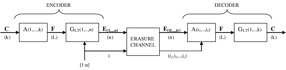
The Raptor code can be viewed as the concatenation of several codes. For example the Raptor encoder specified in [6] is depicted in Fig. 4. The most-inner code is a non systematic Luby-transform (LT) code [17] with input symbols , producing the encoded symbols . The symbols are known as intermediate symbols, and are generated through a pre-coding, made up of some outer high-rate block coding, effected on the symbols . The intermediate symbols are known as LDPC symbols, while the intermediate symbols are known as half symbols. The combination of pre-code and LT code produces a non systematic Raptor code. The parameters and are functions of , according to [6]. Some pre-processing is to be put before the non-systematic Raptor encoding to obtain a systematic one. Such a pre-processing consists in a rate-1 linear code generating the symbols from the information symbols .

LT codes are the first practical implementation of fountain codes. An unique encoded symbol ID (ESI) is assigned to each encoded symbol. Starting from an ESI , the encoded symbol is computed by xor-ing a subset of intermediate symbols. The number , known as the degree associated with the encoded symbol , is a random integer between and : the intermediate symbols are chosen at random according to a specific probability distribution. As a consequence, in order to recover the information symbols the decoder needs both the set of encoded symbols and of the corresponding . This last information can either be explicitly transmitted or obtained by the decoder through the same pseudo-random generator used for the encoding, starting from ESIs, which have therefore to be sent together with the corresponding encoded symbols.
Some of the main properties of LT codes are that the encoder can generate as many encoded symbols as desired and that the decoder is able to recover the block of source symbols from any set of received encoded symbols, whose number is only slightly greater than that of the source symbols (in fact the code claims a low level of overhead). A Raptor code, whose core consists of an LT code, inherit such properties. The addiction of a pre-coding phase is used to obtain an encoding/decoding complexity linear with ; a feature which is missing in the mere LT code.
III-A Fixed-rate Raptor generator matrix
Considering a systematic Raptor code as a finite length linear block code (fixed-rate Raptor code), we can ask what is the structure of its generator matrix. This problem is addressed next for the Raptor code specified in [6]22 2 Throughout this section, the vectors are intended as column vectors (unless explicitly mentioned) and the generator matrix of a linear block code is expressed as a matrix.. The generator matrix of the first pre-coding stage is given by . According to the specifications in [6], consists in columns all of weight equal to , regardless the value of . On the other hand, the generator matrix of the second pre-coding stage is given by , where is a matrix consisting in columns all of constant weight: each column is an element of the Grey sequence of weight , where . Finally, let us denote by the LT code generator matrix (regarded as a finite length linear block code). It is built in such a way that the row of index has ones in positions, where and are derived from the ESI , through pseudo-random algorithms described in in [6]. Next, we use the notation to denote the submatrix of composed of the rows with indexes . The notation is equivalent to .
The intermediate symbols are obtained from as
through the relations
| (4) |
The intermediate symbols are the inputs to the LT encoder for deriving the encoded symbols as
| (7) |
Let us subdivide as
where the sizes of the three submatrices are , and , respectively. If also is subdivided as
that is into two submatrices whose sizes are and , respectively, then the non-systematic Raptor code generator matrix can be expressed as
which satisfies the relation:
Let’s now subdivide into the two submatrices and , whose sizes are and , respectively:
For a systematic code it must be valid the following
and therefore
We have introduced in (III-A) the notations and to denote the first and the last encoded symbols, respectively.
We can state that the pre-processing matrix generating from can be obtained by
and, as a consequence, the systematic Raptor code generator matrix is
| (14) |
In (14) denotes the identity matrix. Obviously, can be inverted if and only if it has full rank . By initializing the random generator of inner LT code through the so-called systematic index (defined in [6]), this property is fulfilled for all .
III-B Raptor Encoding

whereby is a binary matrix called encoding matrix, whose structure is shown in Fig. 5. In this figure, is the identity matrix, is the identity matrix and is the all-zero matrix. The matrix doesn’t properly represent the Raptor code generator matrix (which is defined in (14) instead), but includes the set of constraints imposed by the pre-coding and LT coding together. We use next the notation to indicate the submatrix of obtained by selecting only the rows of with indexes . Again, is equivalent to .
A possible Raptor encoding algorithm exploits a submatrix of . Such a matrix, consisting of the first rows of , is used to obtain solving the system of linear equations:
At this point it is sufficient to multiply by the LT generator matrix to produce the encoded symbols , according to (7).
III-C Raptor Decoding
The most direct way to decode the received sequence lies in inverting each encoding step of Fig. 4; in this case you work on individual sub-codes. When using ML decoding at each sub-code, such a method requires the inversion of a matrix for each code, so it doesn’t appear to be the best solution from the computational viewpoint [18]. Moreover, if the number of received encoded symbols is not larger enough than (which in many cases may mean much higher than) the number of source symbol , it shows an high failure probability.
For example, let’s assume that only a subset of encoded symbols of ESIs are available at the decoder. The first step the decoder should perform is to solve the system of linear equations:
The matrix has size and, obviously, the necessary condition to solve the system is that . If such a condition is not fulfilled, the decoding fails. It means that to recover the source symbols the decoder requires at least encoded symbols (let’s recall that ).
Such a method doesn’t exploit the fact that the intermediate symbols are not independent from each other, but subject to the pre-coding constraints, instead. Therefore, to obtain the intermediate symbols by using a submatrix of (which consider such constraints) turns out to be a far more efficient solution.
According to the above-mentioned assumption, the first decoding step will turn into:
where is a matrix, as defined above. The system can be solved by Gaussian elimination (ML decoding) only if , that is (note that this is a necessary condition for successful ML decoding, not a sufficient one). In this way the number of encoded symbols required at the decoder is definitely lower compared to that in the previous case and, notably, is close to the number of source symbols . Once is known, the source symbols are easily recovered by
To sum up, when the described encoding and decoding algorithms are employed, both the encoding and the decoding are performed by making use of operations which are analogous in the two case (Fig. 6).
III-D Some remarks on the decoding complexity of LDPC and fixed-rate Raptor codes
If we take into consideration the first decoding step, an algorithm to perform GE in a more efficient way on has been proposed in [6, Annex E]. This algorithm share some similarities with that proposed in [4] for LDPC codes. In both cases, the erased symbols are solved by mean of a structured GE, exploiting the sparse nature of the equations to reduce the size of the matrix on which brute-force GE is performed. The targets of the structured GE are for LDPC codes and for Raptor codes. Consider now a LDPC code and its fixed-rate Raptor counterpart. Suppose also an erasure pattern (introduced by the communication channel) leading to a small overhead , i.e., that the amount of correctly received symbols is . On the LDPC code side, the structured GE will be performed on with size . For the Raptor code, the structured GE will work on with size . Hence, while for the LDPC code the complexity of the ML decoder is driven by (i.e., the amount of redundancy, thus by the code rate ), for the Raptor code the complexity depends just on (i.e., it’s code rate independent). The result is that for high rates() LDPC codes have an inherent advantage in complexity. On the other hand, for lower rates Raptor codes shall be preferable.
IV Numerical results
In this section, some numerical results will be provided for LDPC and fixed-rate Raptor codes under ML over the BEC. The performance is provided in terms of codeword error rate (CER) vs. the channel erasure probability . The section is organized in subsections. First, some performance bounds for a linear block code over the BEC are reviewed. Then the performance of some moderate-block-length LDPC codes is provided. The comparison with fixed-rate Raptor codes is presented in a dedicated subsection. Finally, some results for a protograph-based ARA code are given.
IV-A Bounds on the code performance
A lower bound for the CER on the BEC is given by the well-known Singleton bound, which is matched just by an ideal maximum distance separable (MDS) code:
| (15) |
There exist only a few binary codes achieving (15) with equality. An upper bound on the CER for the random code ensembles was introduced by Berlekamp [19]. The bound can be expressed as:
IV-B Moderate block-size LDPC codes
The performance of some moderate-length LDPC codes is provided in Figures 7, 8 and 9. In Figure 7, the CER for a GeIRA code from [3] is presented. The code is picked from an LDPC ensemble with and . The code performance, under ML decoding, tightly approaches the Singleton bound, and pratically matches the Berlekamp bound. The iterative decoding curve, although not so far from the state-of-the-art for iteratively-decoded codes, lies quite far from the bound. The sub-optimality of the IT curve is therefore not due to the code by itself, but to the sub-optimality of the decoder.
The result is confirmed for a family of rate-compatible GeIRA codes with code rates ranging from to and input block size (Figure 8. The higher rates are obtained by puncturing the mother code, which has been derived from the construction proposed in [3]. For the code rates under investigation, the performance is uniformly close to the corresponding Singleton bound, down to low codeword error rates (CER). In Figure 9, the codeword error rate for a is shown. The code is a near-regular GeIRA code with almost constant column weight and feedback polynomial given by . The ML threshold is , while . Also in this case, the error performance curve matches the Berlekamp bound down to low error rates. The minimum distance of this code (and its corresponding multiplicity) has been evaluate by [21]. An error floor estimation has been carried out by mean of the truncated union bound on the codeword error probability, which is given by
| (17) |
where represents the minimum distance multiplicity. Four codewords at have been found, leading to the error floor estimation provided in Figure 9. Even if such results represent only an estimation of the actual error floor, they are quite remarkable. The code performance would in fact deviate remarkably from the Singleton bound just at error rates below .
IV-C Comparisons with fixed-rate Raptor codes
A comparison with fixed-rate Raptor codes specified in the MBMS standard is provided next. In Figure 10, the decoding failure probability (i.e., the CER) as a function of the overhead is depicted for the codes specified in [6] and for some GeIRA codes. The overhead is here defined as the number of codeword symbols that are correctly received in excess respect to (recall that represents the minimum amount of correctly-received bits allowing successful decoding with an ideal MDS code). The comparison is carried out for various block sizes. There is basically no difference in performance between the MBMS Raptor codes and properly-designed LDPC codes under ML decoding. As already pointed out in [22], the decoding failure probability vs. overhead does not seem to depend on the input block size.
A comparison between a (512,256) fixed-rate Raptor code and a near-regular GeIRA code from [3] with constant column weight is provided in Figure 11. In the waterfall region the two codes exhibit almost the same performance. A minimum distance estimation according to [21] was conducted on the two codes. For the (512,256) fixed-rate Raptor code, the minimum distance is given by , with . The lowest Hamming-weight codewords can be obtained by feeding the encoder with the -bits input sequences , where the non-null bits are , , , , , , , , , , , , , , , , , and , , , , , , , , , , , , , , being and the first bit of and , respectively. For the GeIRA code, the estimated minimum distance is , with multiplicity . In both cases, the estimated minimum distance is quite large, and would permit to achieve very low error floors. For the Raptor code, the error floor estimation predicts a deviation from the Berlekamp bound at CER, while for the GeIRA code the error floor would appear at CER. The later result is quite astonishing, and would suggest the use of the near-regular GeIRA construction for applications33 3 Almost all the current wireless systems adopting erasure correcting codes have requirements which are usually much above the error floor of the Raptor code. requiring very low error floors. A final remark on the minimum distance evaluation for fixed-rate Raptor codes. The minimum distance evaluation has been applied to fixed-rate MBMS Raptor codes with various block lengths. For a Raptor code, the lowest-weight codeword found by [21] was (). In the case of a Raptor code, (). Recalling the result for the Raptor code (), it appears from this preliminary analysis that for fixed-rate Raptor codes the minimum distance might scale sub-linearly with the block length.
IV-D ML decoding of a ARA code
In this subsection we provide some numerical results dealing with ML decoding of a ARA code. The ARA protograph ensemble is defined by the base matrix [23]
where the first column corresponds to punctured variable nodes. Its iterative decoding threshold is . The upper bound on the ML threshold is (see Figure 3). The code performance is shown in Figure 12, for both iterative and ML decoding. The gain obtained by the ML decoder in the waterfall region (the error rate performance is actually quite close to the Singleton bound) indicates that the bound on the ML threshold is quite tight. Both the iterative and the ML curves at low error rates present an evident error floor, due to the presence in the codeword set of codewords with Hamming weight .
V Concluding remarks
In this paper we provided some insights on the code design for ML-decoded LDPC on the erasure channel, together with an overview on efficient ML decoding algorithms. The complexity on the decoder side can be kept low with a proper code design. Such approach allows to design codes with a large flexibility in terms of block lengths and code rates. A comparison with ML-decoded fixed-rate Raptor codes (derived from the MBMS specification) has been carried out as well. The results show that LDPC codes under ML decoding can tightly approach the bounds down to very low error rates, even for short block sizes, as their Raptor counterpart. In some cases, the estimated error floor for the LDPC code is much lower than the estimated error floor of the corresponding fixed-rate Raptor code. Since for fixed-rate Raptor codes the error floors are usually very low, the results achieved with the proposed LDPC are astonishing. ML-decoded LDPC codes represent therefore a practical tool to approach the ideal MDS codes performance in many wireless communications contexts, down to very low error rates, and with limited decoding complexity.
VI Acknowledgments
This research was supported, in part, by the University of Bologna Grant Internazionalizzazione, and by the EC-IST SatNEx-II project (IST-27393).
References
- [1] R. G. Gallager, Low-Density Parity-Check Codes. Cambridge, MA: M.I.T. Press, 1963.
- [2] H. D. Pfister, I. Sason, and R. Urbanke, “Capacity-achieving ensembles for the binary erasure channel with bounded complexity,” IEEE Trans. Inform. Theory, vol. 51, no. 7, pp. 2352–2379, July 2005.
- [3] E. Paolini, G. Liva, B. Matuz, and M. Chiani, “Generalized IRA Erasure Correcting Codes for Hybrid Iterative / Maximum Likelihood Decoding,” IEEE Commun. Lett., 2008, accepted for publication.
- [4] D. Burshtein and G. Miller, “An efficient maximum likelihood decoding of LDPC codes over the binary erasure channel,” IEEE Trans. Inform. Theory, vol. 50, no. 11, nov 2004.
- [5] “Framing structure, channel coding and modulation for Satellite Services to Handheld devices (SH) below 3GHz,” Digital Video Broadcasting (DVB),” Blue Book, 2007.
- [6] 3GPP TS 26.346 V7.4.0, “Technical specification group services and system aspects; multimedia broadcast/multicast service; protocols and codecs,” June 2007.
- [7] A. M. Odlyzko, “Discrete logarithms in finite fields and their cryptographic significance,” in Theory and Application of Cryptographic Techniques, 1984, pp. 224–314.
- [8] T. Richardson and R. Urbanke, “Efficient encoding of low-density parity-ceck codes,” IEEE Trans. Inform. Theory, vol. 47, pp. 638–656, Feb. 2001.
- [9] C. Measson, A. Montanari, T. Richardson, and R. Urbanke, “Life above threshold: From list decoding to area theorem and mse,” in Proc. 2004 IEEE Information Theory Workshop, San Antonio, USA, October 2004.
- [10] A. Ashikhmin, G. Kramer, and S. ten Brink, “Extrinsic information transfer functions: Model and erasure channel properties,” IEEE Trans. Inform. Theory, vol. 50, no. 11, pp. 2657–2673, Nov. 2004.
- [11] J. Thorpe, “Low-Density Parity-Check (LDPC) Codes Constructed Protographs,” JPL INP, Tech. Rep. 42-154, Aug. 2003.
- [12] G. Liva and M. Chiani, “Protograph LDPC codes design based on EXIT analysis,” in Proc. IEEE Global Communications Conference (GLOBECOM), Washington, D.C., USA, Nov. 2007.
- [13] A. Abbasfar, K. Yao, and D. Disvalar, “Accumulate repeat accumulate codes,” in Proc. IEEE Globecomm, Dallas, Texas, Nov. 2004.
- [14] G. Liva, E. Paolini, and M. Chiani, “Simple reconfigurable low-density parity-check codes,” IEEE Commun. Lett., vol. 9, no. 3, pp. 258–260, Mar. 2005.
- [15] M. Shokrollahi, “Raptor codes,” IEEE Trans. Inform. Theory, vol. 52, no. 6, pp. 2551–2567, June 2006.
- [16] J. Byers, M. Luby, and M. Mitzenmacher, “A digital fountain approach to reliable distribution of bulk data,” IEEE J. Select. Areas Commun., vol. 20, no. 8, pp. 1528–1540, Oct. 2002.
- [17] M. Luby, “LT codes,” in Proc. of the 43rd Annual IEEE Symposium on Foundations of Computer Science, Vancouver, Canada, Nov. 2002, pp. 271–282.
- [18] M. Luby, M. Watson, T. Gasiba, T. Stockhammer, and W. Xu, “Raptor codes for reliable download delivery in wireless broadcast systems,” in Proc. of 2006 IEEE Consumer Communications and Networking Conf., vol. 1, Jan. 2006, pp. 192–197.
- [19] E. Berlekamp, “The technology of error-correcting codes,” IEEE Proc., vol. 68, pp. 564–593, 1980.
- [20] S. MacMullan and O.M.Collins, “A comparison of known codes, random codes, and the best codes,” IEEE Trans. Inform. Theory, vol. 44, Nov. 1998.
- [21] X.-Y. Hu, M. P. C. Fossorier, and E. Eleftheriou, “On the computation of the minimum distance of low-density parity-check codes,” in Proc. ICC’04, June 2004, pp. 767–771.
- [22] M. Luby, T. Gasiba, T. Stockhammer, and M. Watson, “Reliable multimedia download delivery in cellular broadcast networks,” IEEE Transactions on Broadcasting, vol. 53, pp. 235–246, Mar. 2007.
- [23] G. Liva, S. Song, L. Lan, Y. Zhang, W. Ryan, and S. Lin, “Design of LDPC codes: A survey and new results,” J. Comm. Software and Systems, Sept. 2006.


