Stabilisation of long-period periodic orbits using time-delayed feedback control
Abstract
The Pyragas method of feedback control has attracted much interest as a method of stabilising unstable periodic orbits in a number of situations. We show that a time-delayed feedback control similar to the Pyragas method can be used to stabilise periodic orbits with arbitrarily large period, specifically those resulting from a resonant bifurcation of a heteroclinic cycle. Our analysis reduces the infinite-dimensional delay-equation governing the system with feedback to a three-dimensional map, by making certain assumptions about the form of the solutions. The stability of a fixed point in this map corresponds to the stability of the periodic orbit in the flow, and can be computed analytically. We compare the analytic results to a numerical example and find very good agreement.
keywords
Feedback control, heteroclinic cycle, delay equation.AMS
37C27, 37C29.1 Introduction
The stabilisation of unstable periodic orbits (UPOs) using feedback control has attracted the attention of many authors over a number of years. The time-delayed feedback method of Pyragas [1], has been of particular interest. Here, the feedback is proportional to the difference between the current and a past state of the system. Specifically, where is some state vector, is the period of the targeted UPO and is a feedback gain matrix. Advantages of this method include the following. First, since the feedback vanishes on any orbit with period , the targeted UPO is still a solution of the system with feedback. Control is therefore achieved in a non-invasive manner. Second, the only information required a priori is the period of the target UPO, rather than a detailed knowledge of the profile of the orbit, or even any knowledge of the form of the original ODEs, which may be useful in experimental setups. The method has been implemented successfully in a variety of laboratory situations [2, 3, 4, 5, 6, 7, 8], as well as analytically and numerically in spatially extended pattern-forming systems [9, 10, 11, 12]; more examples can be found in a recent review by Pyragas [13].
Until now, there has been little or no study on whether there are limitations to Pyragas feedback control as the period of the targeted orbit, and hence the delay time, becomes large. In this paper, we investigate the use of Pyragas feedback on unstable periodic orbits with arbitrarily large period.
One mechanism for the generation of long-period periodic orbits is at bifurcations from homoclinic orbits or heteroclinic cycles. In this paper we focus on a subcritical bifurcation from a symmetric heteroclinic cycle, specifically the heteroclinic cycle of Guckenheimer and Holmes [21]. The bifurcation produces a branch of unstable long-period periodic orbits and we investigate using a time-delayed feedback control similar to the Pyragas feedback as a stabilisation mechanism.
The addition of Pyragas feedback to the ODEs considered by Guckenheimer and Holmes results in an infinite-dimensional delay equation. In order to analyse trajectories near the periodic orbit of interest, we make a number of assumptions about the form of solutions to the delay-differential equation and reduce the flow to a three-dimensional map. This method, after the assumptions have been made, is a modified version of the standard ‘small box and Poincaré map’ analysis used by many authors to study the dynamics of trajectories close to heteroclinic cycles. This reduction of an infinite-dimensional delay equation to a finite dimensional map has not appeared before in the literature. Although our assumptions are not fully rigorously justified, we test the validity of our arguments by comparing our results with a numerical example. We find excellent agreement between the analytical and numerical results. A surprising result of the analysis for the particular example we use is that as the period of the orbit increases, the amplitude of the gain parameter required to stabilise the unstable orbits decreases.
This paper is organised as follows. In section 2 we give a review of heteroclinic cycles and their bifurcations. We describe the Guckenheimer–Holmes heteroclinic cycle, and summarise the standard approach to analysing trajectories close to heteroclinic cycles. In section 3 we describe how we choose the feedback control terms which are added to the equations. We then perform the reduction of the equations described above, which gives us a method of computing the stability of the periodic orbits. Section 4 contains numerical examples and section 5 concludes.
2 Review of heteroclinic cycles
A heteroclinic cycle is a topological circle of connecting orbits between at least two saddle-type equilibria. In generic (non-symmetric) dynamical systems, heteroclinic cycles are of high codimension and their existence for open sets of parameter values is unexpected. If a dynamical system contains flow-invariant subspaces, the connecting orbits can be contained within these subspaces, and then the heteroclinic cycle is robust to perturbations of the system that preserve the invariance of these subspaces. Flow invariant subspaces can arise due to symmetry, or due to other restrictions on the flow (such as extinctions in population dynamics models [14]). The review of Krupa [15] contains many examples of robust heteroclinic cycles. In this paper we consider robust heteroclinic cycles in symmetric systems.
2.1 Preliminary definitions
Consider a continuous-time dynamical system defined by an ODE:
| (1) |
where is a -equivariant vector field, that is,
| (2) |
and is a finite Lie group. An equilibrium of (1) satisfies . We consider only hyperbolic equilibria, and assume that is smoothly linearisable about each equilibrium.
Definition 1.
A heteroclinic cycle is an invariant set consisting of the union of a set of equilibria and orbits , where is a heteroclinic connection between and ; and . We require that . If , then is a homoclinic orbit. A heteroclinic cycle is a homoclinic cycle if there exists such that for all .
For we define the isotropy subgroup ,
| (3) |
For an isotropy subgroup of , we define the fixed-point subspace
| (4) |
Definition 2.
A heteroclinic cycle is robust if for each , , there exists a fixed-point subspace, where and
- 1.
is a saddle and is a sink for the flow restricted to ,
- 2.
there is a heteroclinic connection from to contained in .
Robust heteroclinic cycles occur as codimension-zero phenomena in systems with symmetry. That is, they can exist for open sets of parameter values. Bifurcations of heteroclinic cycles therefore occur as codimension-one phenomena. We now consider the computation of the stability of heteroclinic cycles and the associated bifurcations.
2.2 Resonant bifurcations
The stability of a heteroclinic cycle is usually computed by constructing Poincaré maps on a Poincaré section of the flow. The flow near the cycle is divided into two parts; the ‘local’ part, near the equilibria, where the flow can be well approximated by the linearised flow about the equilibria, and the ‘global’ part of the flow, where the trajectory is away from the equilibria. The global part of the flow occurs on a much faster timescale than the local part and can be approximated by a linearisation of the flow around the heteroclinic connections. The construction of such Poincaré maps is a standard procedure, details can be found in, for example [16, 17].
Heteroclinic cycles generically lose stability in two ways: resonant bifurcations and transverse bifurcations. Transverse bifurcations occur when one of the eigenvalues at an equilibrium passes through zero; the equilibrium undergoes a local bifurcation. We do not consider transverse bifurcations here, see [18] for details. Throughout this paper, when we refer to ‘the eigenvalues at an equilibrium’, we of course mean the eigenvalues of the Jacobian matrix of the flow linearised about that equilibrium.
At a resonant bifurcation the eigenvalues at the equilibria are generically non-zero, but satisfy an algebraic condition that determines a global change in the stability properties of the cycle. Resonant bifurcations were first studied in the non-symmetric case by Chow et al. [19] in the context of a bifurcation from a homoclinic orbit. A more recent study [20] considers a codimension-two resonant bifurcation from a robust heteroclinic cycle with complex eigenvalues.
Resonant bifurcations are generically accompanied by the birth or death of a long-period periodic orbit. If is the bifurcation parameter controlling the resonant bifurcation (that is, at the bifurcation point), then the period of the bifurcating periodic orbit generically scales as
Resonant bifurcations can occur in a supercritical or subcritical manner. We consider the subcritical case, when the branching periodic orbits are unstable, and in the following show that Pyragas-type time-delayed feedback can stabilise the periodic orbits. Our analysis focuses on the Guckenheimer–Holmes cycle in .
2.3 The Guckenheimer–Holmes cycle
The Guckenheimer–Holmes cycle [21] is a prototypical example of a robust heteroclinic cycle. We use this cycle as an example on which to base our analysis. First we review the original case with no feedback.
The equations considered by Guckenheimer and Holmes can be written:
| (5) |
where , and and are real parameters. The equations are equivariant under the symmetry group , generated by a reflection and a rotation :
We label the equilibrium on the positive -axis as . Here, and throughout the remainder of the paper, subscripts on equilibria, coordinates and similar objects should be taken mod . Each two-dimensional coordinate plane is a fixed point subspace. If , then the only equilibria in each coordinate plane are those lying on the coordinate axes. We consider the case and then it can be shown that in the plane , is a saddle and is a sink. It can additionally be shown that in forward time trajectories are bounded away from infinity and therefore by the Poincaré –Bendixson theorem there exists a heteroclinic connection from to . Similarly, connections also exist from to , and to . These connections lie in two-dimensional fixed-point subspaces (the two-dimensional coordinate planes), so the cycle is robust. The resulting heteroclinic cycle is shown schematically in figure 1. Also note that , so the cycle is homoclinic.

The stability of the cycle can be calculated using the methods described above. It is a standard procedure, but we outline the method here, as we use similar ideas later when considering the stability of periodic orbits in the system with added time-delayed feedback. Consider a trajectory which passes close to the equilibrium . The linearised flow near is:
| (6) | ||||
| (7) | ||||
| (8) |
The direction is the ‘radial’ direction, and as shown in [22], for heteroclinic cycles of this type, the radial direction does not affect the stability of the cycle. All trajectories move away from the origin, and also away from infinity, and in this case are attracted to an ‘invariant sphere’ [23] which contains the heteroclinic cycle. Therefore, for simplicity, we henceforth ignore this component. We define Poincaré sections close to :
| (9) | ||||
| (10) |
where , and construct a Poincaré return map on . Consider a trajectory which passes through at time with . The trajectory will hit at
with
We thus write down a local map , which describes the flow near the equilibria:
| (11) |
The flow near the heteroclinic connection from to a plane near is approximated by the global map :
| (12) |
where is the coordinate of the trajectory when it next hits , and is a positive constant. Note that the constant term in this expansion of is zero because the plane is invariant. We write . Since , the map is a return map on . Write and then the return map is
where .
The map has fixed points at and at . The fixed point at corresponds to the heteroclinic cycle in the flow and is stable if . The heteroclinic cycle loses stability in a resonant bifurcation at . The second fixed point at corresponds to a branch of periodic orbits, as long as is small and positive. The symmetry acts as a spatio-temporal symmetry on the periodic orbits. That is, if we write the periodic solution as a trajectory , with minimal period , then
The stability of the orbits can be determined by finding the stability of the fixed point in the map . It is simple to see that if , is small and positive (and hence corresponds to a periodic orbit in the flow) when , so the resonant bifurcation is subcritical. We find that
and so is unstable. Conversely, if , then corresponds to a branch of stable periodic orbits if , and the bifurcation is supercritical. The period of the orbit is approximately
where and is the time spent by the trajectory each time it passes close to an equilibrium. We are ignoring the time spent away from the equilibria (that is, close to the heteroclinic connections in the invariant planes) since it is much less than when we are close to the resonant bifurcation, that is, .
In equations (5), the resonant heteroclinic bifurcation at is degenerate. That is, the branch of periodic orbits exists only at . This corresponds to the case in the map . We add additional higher order terms to break this degeneracy, specifically we consider
| (13) |
The additional terms preserve the equilibria and the symmetries of the system, and also the invariant planes and the heteroclinic cycle. The heteroclinic cycle still loses stability in a resonant bifurcation at , but now a branch of periodic orbits is created in either or . The sign of determines the branching direction and whether, in the map , is greater or less than . If , we see a branch of unstable periodic orbits in (and the resonant bifurcation is subcritical). If , we see a branch of stable periodic orbits in (and the bifurcation is supercritical). A complete study of the effect of fifth order terms on the dynamics near the GH cycle has not been performed. However, the above assertion can be seen by considering the effect of the new term on the component when the trajectory is close to the plane but away from either coordinate axis.
In the following, we consider the subcritical case, where the periodic orbits are unstable, and add non-invasive time-delayed feedback to stabilise the orbits near the heteroclinic cycle.
3 Addition of feedback terms
3.1 Choice of coordinates
To ease analysis and improve the accuracy in the numerical computations in section 4, we introduce new coordinates . Along with a change in timescale, this transforms equations (13) to
| (14) |
where . Note that in these coordinates, the equilibria are at, e.g. , . The invariant planes in the coordinates are transformed to . However, we are not interested in trajectories which lie in the coordinate planes, only those which are close to them.
3.2 Addition of feedback
Pyragas feedback is additive and has the form where is a (real) gain matrix and is the period of the targeted periodic orbit. Our choice of coordinates suggests the following slightly altered functional form for the feedback:
| (15) |
For trajectories close to the periodic orbit, and so the feedback terms are approximately of Pyragas form. For this choice of feedback, the equilibria and the invariance of the coordinate planes (in the original coordinates) are preserved. However, we additionally choose to use the symmetries of the system to make a further change in the form of the feedback which simplifies the subsequent analysis. The feedback we use is:
| (16) |
where is one-third of the period of the orbit. Due to the spatiotemporal symmetry of the periodic orbit under the action of , the feedback vanishes at the periodic orbit, and so the periodic orbit is still a solution of the system. However, this feedback does not preserve the equilibria or invariant planes (in the original coordinates).
We choose the matrix in a similar manner to that in [24], as follows. We write
where
| (17) |
The matrix has the form of the feedback matrix used by Fiedler et al.[25] in a two-dimensional example; stabilising periodic orbits emanating from a subcritical Hopf bifurcation. Recall that the orbit has two unstable directions, and one stable direction — the radial direction. The matrix is chosen so the feedback is rotated to align with the unstable directions, and there is no feedback in the stable direction.
The resulting equations with feedback are
| (18) |
where
3.3 Stability analysis
We analyse the stability of the periodic orbits close to the heteroclinic cycle in a similar manner to the methods used without feedback. We assume we are close to the resonant bifurcation, that is, , so that the periodic orbit lies close to the heteroclinic cycle, and consider the flow close to the periodic orbit. The linearised equations close to the equilibrium are given by:
| (19) | ||||
| (20) |
where the are the components of the feedback gain matrix . As before we neglect the equation — since the feedback only acts in directions tangent to the plane containing the periodic orbit, we assume that when trajectories are close enough to the periodic orbit the dynamics in the radial direction are unaffected. That is, near , the direction will be contracting and so not affect the stability of the orbit. In section 4.1 we show numerical results which support this assumption.
Recall that the periodic orbits we are attempting to stabilise are spatiotemporally symmetric under the action of . We make use of this in the following. At each equilibrium, we define a contracting direction, and an expanding direction. At , the contracting direction is the direction, and the expanding direction is the direction.
Unlike in the case without feedback, we cannot solve the linear equations explicitly, and so we make the following approximations. Let be the periodic orbit for the original system (in the logarithmic coordinates). Then is still a solution of the system with feedback. Consider solving the delay differential equation for the system with feedback for a trajectory which starts close to . That is, for , is close to . Then for , the feedback terms in the delay differential equation will be small, that is, the equations will only be a small perturbation from the original system. By continuity, the solution for will also be close to .
Set as the trajectory intersects the plane (, for , ) on the th time the trajectory passes close to an equilibrium, . With no feedback, the local part of the trajectory can be written down exactly. The expanding and contracting components, and satisfy:
| (21) | ||||
| (22) |
for , where is the length of time spent near the equilibrium (i.e. in the small box) and is the expanding coordinate of the trajectory as it intersects the plane .
For the system with feedback, we cannot explicitly solve the linearised equations. Given the argument above, we assume that we start sufficiently close to the periodic orbit that solutions are only a small perturbation away from those for the case with no feedback. That is, we write, for ,
| (23) | ||||
| (24) |
where and are functions which satisfy
and if the trajectory is exactly the periodic orbit, . We will use this assumed form of the local flow together with equations (19) and (20) and the global flow as before to derive a new return map. This gives recurrence relations for , and the functions and . Figure 2 shows a schematic of the local flow past an equilibrium , in the original coordinates.

We again ignore the time the trajectory spends near the heteroclinic connections but away from the equilibria, so for , the flow is given by
| (25) | ||||
| (26) |
Using the symmetry , we can rewrite the linear equations (19) and (20) as
| (27) | ||||
| (28) |
where the delayed terms are the corresponding coordinates near the previous equilibrium, that is
| (29) | ||||
| (30) |
The time of flight of the trajectory between the planes and , , will not be equal to the delay time except when the trajectory is exactly on the periodic orbit (see figure 2). In order to find the coordinates at , we assume the flow given by (25) and (26) is also valid for . The coordinates of the trajectory at are therefore:
| (31) | ||||
| (32) |
Writing , where (since we are close to the periodic orbit) and expanding and about zero gives
| (33) | ||||
| (34) |
since . Substituting into (31) and (32) gives:
| (35) | ||||
| (36) |
We also have that for ,
Substituting (23), (24), (35) and (36) into equations (27) and (28) we find:
| (37) |
| (38) |
These expressions are true for all , so we set to simplify and find:
| (39) | ||||
| (40) |
that is, a recurrence relation for and if the and are known. We write , and to further simplify:
| (41) | ||||
| (42) |
We next find an expression for which we use to find a recurrence relation for the . Recall that , so from (23) we have
| (43) | ||||
| (44) |
In order to be able to get tractable results in what follows, we need to invert the above equation for . Motivated by numerical results, which we give in section 4.1, we make the following assumption:
that is, that is approximately a linear function of . Using this gives us
so
| (45) |
where .
We make a similar assumption on the , that is, , and then use (24) to find :
which is an expression for the local map . We assume that the global map is of the same form as the case without feedback (12) when we are close enough to the periodic orbit, and hence find a return map for the :
Substituting equation (45) into equations (41) and (42) results in a third order recurrence system:
| (46) |
Note that when , the recurrence relation reduces to that for the system with no feedback, as expected. This system of three recurrence relations has a fixed point at
which corresponds to the periodic orbit in the flow. The stability of the fixed point in the recurrence relation will correspond to the stability of the periodic orbit in the flow.
The Jacobian matrix of (46) at this fixed point is:
where . The characteristic equation of is
| (47) |
where
| (48) | ||||
| (49) | ||||
| (50) |
The fixed point will be unstable if (47) has any solutions with , so curves with define stability boundaries of the periodic orbit. Recall that and is a function of just two parameters, and . We consider the stability of the periodic orbit as the parameters and are varied.
3.4 Determination of stability boundaries
We split our investigation of the stability boundaries into three cases. We introduce the bifurcation parameter . Without feedback, the heteroclinic cycle is stable in and the periodic orbits exist and are unstable in . We consider analytically the limits of the stability boundary curves as . The boundaries can actually be computed exactly (although the algebra is rather nasty), since the eigenvalues are the roots of a cubic. We plot the boundaries for specific parameter values in figure 3. In section 4 we compute the stability of the periodic orbit in the original system (18), numerically using the continuation package dde-biftool.
Case 1:
A stability boundary with corresponds to a steady state bifurcation of the periodic orbit. This occurs when , that is
It can easily be computed that
| (51) | ||||
| and | ||||
| (52) | ||||
In the limit , using , we find
| (53) |
It is also simple to calculate that in the limit the eigenvalue which goes through as this curve is crossed is greater than if and less than if .
Case 2:
A stability boundary with will correspond to a period-doubling bifurcation of the periodic orbit. These curves will have , that is,
Again, we can compute the coefficients
| (54) | ||||
| (55) |
and in the same limit as above, we find
| (56) |
so there are two solutions for some function of , and . The direction of the bifurcation as these lines are crossed in this case depends on .
Case 3: ,
For , , it can easily be computed that we must have . The computations in this case are messier, so we omit them, and give the resulting curve in the limit ,
| (57) |
The direction of the bifurcation again will depend on .
The curves (53), (56) and (57) describe the limiting cases of the stability boundaries of the periodic orbit as the point is approached. Since the characteristic polynomial (47) is cubic, it can be solved for any values of and . In figure 3 we plot the solutions of (47) for a specific set of parameter values. In this case only the curves corresponding to and are stability boundaries. The lower boundary is the quadratic curve for and the left hand boundary is a straight line corresponding to . The remaining curves with do not form stability boundaries in this case because the periodic orbit is already unstable in the regions in which they exist.
We can see that for these parameter values, the periodic orbit is stable for a wide range of parameters, and specifically, can be stabilised arbitrarily close to the heteroclinic cycle, that is, for arbitrarily large period. That is, for any we can find a for which the periodic orbit is stable. In fact, for this particular case, we see that as gets smaller, in order for the orbit to be stable, we have to choose , the gain parameter, to be increasingly small. This seems a rather surprising result - that as the period of the targeted orbit increases, the amplitude of the gain parameter tends towards zero.

3.5 Stability of the heteroclinic cycle
We note that the recurrence relations (46) have a second solution, , , , which corresponds to the heteroclinic cycle. We can consider the stability of this solution by considering the solutions to (47) in the limit . In this limit, , and . The cubic equation (47) therefore has one solution with and two solutions with . Therefore this fixed point is always unstable in the recurrence relation, and so the heteroclinic cycle is always unstable in the flow.
4 Numerical results
We use the Matlab package dde-biftool [26] to numerically analyse the stability of periodic orbits in the system (18). The delay time was set equal to the period of the bifurcating periodic orbits (and so is a function of ), and was calculated numerically from the system with no feedback. Parameters used were the same as those used to produce figure 3.
Figure 4 shows a contour plot of the amplitude of the largest Floquet multiplier as the parameters and are varied. The periodic orbit is stable when all Floquet multipliers have amplitude less than , and this region is indicated by the shading in figure 4. Comparison with figure 3, showing the stability as calculated analytically, shows a very good agreement between the location of the stability boundaries. The shapes of the boundaries also agrees, that is, the left hand boundary is a straight line, whereas the lower boundary is part of a parabola.

The nature of the bifurcations that occur as the boundaries are crossed also agrees with the analytical result. That is, the left hand boundary is a period-doubling bifurcation, with a critical Floquet multiplier equal to , and the lower boundary is a steady state bifurcation with a critical Floquet multiplier of .
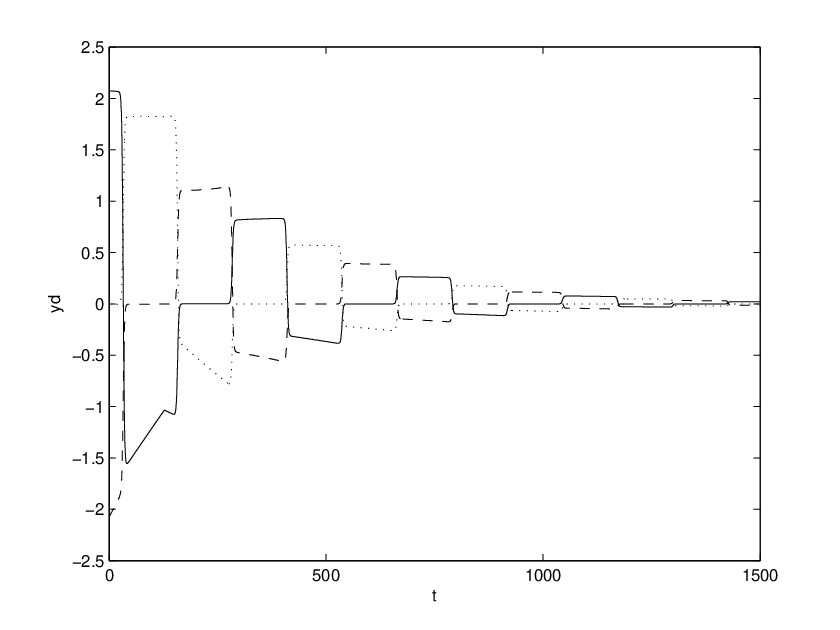
Forward integration of the equations (18) also confirms the stability results. In figure 5 we show results from such an integration. We also show the derivative of the coordinates and the feedback terms. It can be seen that as the periodic orbit is approached, the derivative of the expanding coordinate tends to (in this case, ), and the feedback terms tend towards zero.


4.1 Justification of assumptions
In section 3.3 we make a number of assumptions regarding the form of solutions to the delay differential equations. Firstly, we assume that the ‘radial’ direction does not affect the stability of the periodic orbits, and so we neglect this coordinate in our construction of a Poincaré map. Secondly, that trajectories starting near the periodic orbits will be only small perturbations from the form of solutions to the original equations without feedback. Thirdly, we make the assumption that , and .
Here, we address each assumption in turn and show that our numerical results support these assumptions.
Figure 5(c) shows the feedback terms in a forward integration of equations (18) as the periodic orbit is approached. It can be seen here that the feedback terms corresponding to the radial direction are much smaller than the other feedback terms — on this scale they cannot be distinguished from zero. Hence the affect of the feedback on the radial direction is negligible and this assumption is justified.
Regarding the second assumption, it can be clearly seen in figure 5(c) that the feedback terms decay to zero as the periodic orbit is approached. However, this is to be expected in the case that the periodic orbit is stable. In figure 6 we show the results of an integration in which the periodic orbit is unstable. It can be seen from the time series in 6(a) that the trajectories still remain approximately of the form of the periodic orbit even though the trajectory is moving away. Figure 6(b) shows the feedback terms, a measure of how close the trajectory is to the periodic orbit. Although they are increasing in magnitude, they do so in the same manner one would expect for an unstable periodic orbit in ordinary differential equations. That is, by starting trajectories close enough to the periodic orbit, the feedback magnitude can be bounded above for arbitrarily long time.


The third assumption is that that , and . Note that in the recurrence relations (46), the terms in only appear in the combination (similarly with in the combination ). Therefore, we only need to show that the difference between and is much smaller than to justify our assumption (and similar for the ). For the integration we perform for figure 5(a) we compute the values of , and (and the corresponding values for ) on each pass the trajectory makes past an equilibrium. We plot these values in figure 7. It can be seen that the difference between and (and between and ) is clearly very small, and is much less than () for this example.


5 Discussion
We have shown that a time-delayed feedback control mechanism similar to that first introduced by Pyragas can be used to stabilise periodic orbits of arbitrarily large period, specifically those resulting from a resonant bifurcation from a heteroclinic cycle. Our analytical results are based on a analysis of the stabilisation of orbits near the Guckenheimer–Holmes cycle. These results are asymptotic, that is, they are correct in the limit of the periodic orbit being close to the heteroclinic cycle. However, in comparison with numerical results (which conversely, are much harder to obtain when the orbit is close to the cycle due to the long period of the orbit), the results actually agree for some large(ish) range of parameters away from the bifurcation point.
It should also be possible to extend this analysis so that it applies to resonant bifurcations from higher dimensional heteroclinic cycles. However, care may need to be taken with the transverse eigenvalues.
As the resonant bifurcation is approached, the period of the bifurcating periodic orbit grows like , where is the bifurcation parameter. This is in contrast to the homoclinic bifurcation, in which case the bifurcating periodic orbit has a period which grows like . This difference in scaling between the growth rate of the periods of the orbits indicates that the results of adding similar time-delayed feedback near a subcritical homoclinic bifurcation may be quite different to the results given here. Work on this problem is ongoing.
Acknowledgments
The author would like to thank Mary Silber for many useful discussions regarding this work, and David Barton for assistance using dde-biftool. Two anonymous referees also provided some helpful comments. This work was supported in part by grant NSF-DMS-0709232.
References
- [1] K. Pyragas, Continuous control of chaos by self-controlling feedback, Phys. Letts. A, 170 (1992), 421–428.
- [2] K. Pyragas and A. Tamaševičius, Experimental control of chaos by delayed self-controlling feedback, Phys. Letts. A, 180 (1993), 99.
- [3] D. J. Gauthier, D. W. Sukow, H. M. Concannon and J. E. S. Socolar, Stabilizing unstable periodic orbits in a fast diode resonator using continuous time-delay autosynchronization, Phys. Rev. E, 50 (1994), 2343.
- [4] S. Bielawski, D. Derozier and P. Glorieux, Controlling unstable periodic orbits by a delayed continuous feedback, Phys. Rev. E, 49 (1994), R971.
- [5] Th. Pierre, G. Bonhomme and A. Atipo Controlling the Chaotic Regime of Nonlinear Ionization Waves using the Time-Delay Autosynchronization Method, Phys. Rev. Lett., 76 (1996), 2290.
- [6] T. Fukuyama, H. Shirahama and Y. Kawai, Dynamical control of the chaotic state of the current-driven ion acoustic instability in a laboratory plasma using delayed feedback, Physics of Plasmas, 9 (2002), 4525.
- [7] F. W. Schneider, R. Blittersdorf, A. Förster, T. Hauck, D. Lebender and J. Müller, Continuous Control of Chemical Chaos by Time Delayed Feedback, J. Phys. Chem., 97 (1993), 12244.
- [8] A. Lekebusch, A. Förster and F. W. Schneider, Chaos Control in an Enzymatic Reaction, J. Phys. Chem., 99 (1995), 681.
- [9] M. E. Bleich, J. E. S. Socolar, Controlling spatiotemporal dynamics with time-delay feedback Phys. Rev. E, 54(1) (1996).
- [10] K. Montgomery and M. Silber, Feedback Control of Traveling Wave Solutions of the Complex Ginzburg Landau Equation, Nonlinearity, 17(6) (2004), 2225-2248.
- [11] W. Lu, D. Yu, R. G. Harrison, Control of patterns in spatiotemporal chaos in optics, Phys. Rev. Letts., 76(18) (1996), 3316–3319.
- [12] C. M. Postlethwaite and M. Silber, Spatial and temporal feedback control of traveling wave solutions of the two-dimensional complex Ginzburg–Landau equation, Physica D, 236 (2007), 65–74.
- [13] K. Pyragas, Delayed feedback control of chaos, Phil. Trans. R. Soc. A, 364 (2006), 2309–2334.
- [14] J. Hofbauer and K. Sigmund, Evolutionary Games and Population Dynamics (1998), CUP.
- [15] M. Krupa, Robust heteroclinic cycles J. Nonlinear Sci., 7 (1997), 129-176.
- [16] V. Kirk and M. Silber, A Competition between heteroclinic cycles Nonlinearity, 7 (1994), 1605-1621.
- [17] M. Krupa and I. Melbourne, Asymptotic stability of heteroclinic cycles in systems with symmetry. II, Proc. Roy. Soc. Ed. A, 134 (2004), 1177–1197
- [18] P. Chossat, M. Krupa, I. Melbourne and A. Scheel, Transverse bifurcations of homoclinic cycles Physica D, 100 (1997), 85-100.
- [19] S.-N. Chow, B. Deng and B. Fielder, Homoclinic bifurcation at resonant eigenvalues, J. Dyn. Diff. Eq., 2 (1990), 177-244.
- [20] C. M. Postlethwaite and J. H. P. Dawes, A codimension-two resonant bifurcation from a heteroclinic cycle with complex eigenvalues. Dynamical Systems: An International Journal, 21(3) (2006), 313-336.
- [21] J. Guckenheimer and P. Holmes, Structurally stable heteroclinic cycles. Math. Proc. Camb. Phil. Soc., 103 (1988), 189-192.
- [22] M. Krupa and I. Melbourne, Asymptotic stability of heteroclinic cycles in systems with symmetry, Erg. Th. Dyn. Sys., 15 (1995) 121–147.
- [23] M. J. Field Lectures on bifurcations, dynamics and symmetry, Pitman Research Notes in Mathematics, 356 (1996).
- [24] C. M. Postlethwaite and M. Silber, Stabilizing unstable periodic orbits in the Lorenz equations using time-delayed feedback control, PRE, 76 (2007), 056214
- [25] B. Fiedler, V. Flunkert, M. Georgi, P. Hovel and E. Scholl, Refuting the odd number limitation of time-delayed feedback. Phys. Rev. Lett., 98 (2007), 114101.
- [26] K. Engelborghs, T. Luzyanina, G. Samaey, DDE-BIFTOOL v. 2.00: a Matlab package for bifurcation analysis of delay differential equations, Technical Report TW-330, Department of Computer Science, K. U. Leuven, Leuven, Belgium, 2001.