跳到论文正文
W Papers独立论文阅读器 arXiv:0804.2887 论文正文 计算阅读时间 · 0%
引用这篇论文根据当前论文元数据生成,正式投稿前建议核对。


License: arXiv.org perpetual non-exclusive license
arXiv:0804.2887v2 [math.DS] 06 Jun 2008

Hitting Time Statistics and Extreme Value TheoryThanks: JMF is partially supported by POCI/MAT/61237/2004 and MT is supported by FCT grant SFRH/BPD/26521/2006. All three authors are supported by FCT through CMUP

Ana Cristina Moreira Freitas Address: Ana Cristina Moreira Freitas
Centro de Matemática & Faculdade de Economia da Universidade do Porto
Rua Dr. Roberto Frias
4200-464 Porto
Portugal
Email address: amoreira@fep.up.pt
, Jorge Milhazes Freitas Address: Jorge Milhazes Freitas
Centro de Matemática da Universidade do Porto
Rua do Campo Alegre 687
4169-007 Porto
Portugal
Email address: jmfreita@fc.up.pt URL: http://www.fc.up.pt/pessoas/jmfreita
and Mike Todd Address: Mike Todd
Centro de Matemática da Universidade do Porto
Rua do Campo Alegre 687
4169-007 Porto
Portugal
Email address: mtodd@fc.up.pt URL: http://www.fc.up.pt/pessoas/mtodd
Date: August 24, 2026
Abstract.

We consider discrete time dynamical systems and show the link between Hitting Time Statistics (the distribution of the first time points land in asymptotically small sets) and Extreme Value Theory (distribution properties of the partial maximum of stochastic processes). This relation allows to study Hitting Time Statistics with tools from Extreme Value Theory, and vice versa. We apply these results to non-uniformly hyperbolic systems and prove that a multimodal map with an absolutely continuous invariant measure must satisfy the classical extreme value laws (with no extra condition on the speed of mixing, for example). We also give applications of our theory to higher dimensional examples, for which we also obtain classical extreme value laws and exponential hitting time statistics (for balls). We extend these ideas to the subsequent returns to asymptotically small sets, linking the Poisson statistics of both processes.

Key words and phrases: 
Return Time Statistics, Extreme Value Theory, Non-uniform hyperbolicity, Interval maps
2000 Mathematics Subject Classification
37A50, 37C40, 60G10, 60G70, 37B20, 37D25, 37E05

1. Introduction

In this paper we demonstrate and exploit the link between Extreme Value Laws (EVL) and the laws for the Hitting Time Statistics (HTS) for discrete time non-uniformly hyperbolic dynamical systems.

The setting is a discrete time dynamical system (𝒳,ℬ,μ,f)(\mathcal{X},\mathcal{B},\mu,f), where 𝒳\mathcal{X} is a dd-dimensional Riemannian manifold, ℬ\mathcal{B} is the Borel σ\sigma-algebra, f:𝒳→𝒳f:\mathcal{X}\to\mathcal{X} is a measurable map and μ\mu an ff-invariant probability measure (for all A∈ℬA\in\mathcal{B} we have μ⁡(f−1​(A))=μ⁡(A)\mu(f^{-1}(A))=\mu(A)). We consider a Riemannian metric on 𝒳\mathcal{X} that we denote by ‘dist’ and for any ζ∈𝒳\zeta\in\mathcal{X} and δ>0\delta>0, we define Bδ​(ζ)={x∈𝒳:dist​(x,ζ)<δ}B_{\delta}(\zeta)=\{x\in\mathcal{X}:\mbox{dist}(x,\zeta)<\delta\}. Also let Leb{\rm Leb} denote Lebesgue measure on 𝒳\mathcal{X} and for every A∈ℬA\in\mathcal{B} we will write |A|:=Leb⁡(A)|A|:={\rm Leb}(A). The measure μ\mu will be an absolutely continuous invariant probability measure (acip) with density denoted by ρ=d​μd​Leb\rho=\frac{d\mu}{d{\rm Leb}} . We will denote ℝ+:=(0,∞)\mathbb{R}^{+}:=(0,\infty) and ℝ0+:=[0,∞)\mathbb{R}_{0}^{+}:=[0,\infty).

1.1. Extreme Value Laws

In this context, by EVL we mean the study of the asymptotic distribution of the partial maximum of observable random variables evaluated along the orbits of the system. To be more precise, take an observable φ:𝒳→ℝ∪{±∞}\varphi:\mathcal{X}\to\mathbb{R}\cup\{\pm\infty\} achieving a global maximum at ζ∈𝒳\zeta\in\mathcal{X} (we allow φ⁡(ζ)=+∞\varphi(\zeta)=+\infty) and consider the stationary stochastic process X0,X1,…X_{0},X_{1},\ldots given by

Xn=φ∘fn,for each n∈ℕ.X_{n}=\varphi\circ f^{n},\quad\mbox{for each }n\in{\mathbb{N}}. (1.1)

Define the partial maximum

Mn:=max⁡{X0,…,Xn−1}.M_{n}:=\max\{X_{0},\ldots,X_{n-1}\}. (1.2)

If μ\mu is ergodic then Birkhoff’s law of large numbers says that Mn→φ⁡(ζ)M_{n}\to\varphi(\zeta) almost surely. Similarly to central limit laws for partial sums, we are interested in knowing if there are normalising sequences {an}n∈ℕ⊂ℝ+\{a_{n}\}_{n\in\mathbb{N}}\subset\mathbb{R}^{+} and {bn}n∈ℕ⊂ℝ\{b_{n}\}_{n\in\mathbb{N}}\subset\mathbb{R} such that

μ⁡({x:an​(Mn−bn)≤y})=μ⁡({x:Mn≤un})→H⁡(y),\mu\left(\{x:a_{n}(M_{n}-b_{n})\leq y\}\right)=\mu\left(\{x:M_{n}\leq u_{n}\}\right)\to H(y), (1.3)

for some non-degenerate distribution function (d.f.) HH, as n→∞n\to\infty. Here un:=un​(y)=y/an+bnu_{n}:=u_{n}(y)=y/a_{n}+b_{n} is such that

n​μ​(X0>un)→τ, as n→∞,n\mu(X_{0}>u_{n})\to\tau,\;\mbox{ as $n\to\infty$,} (1.4)

for some τ=τ⁡(y)≥0\tau=\tau(y)\geq 0 and in fact H⁡(y)=H⁡(τ⁡(y))H(y)=H(\tau(y)). When this happens we say that we have an Extreme Value Law (EVL) for MnM_{n}. Note that, clearly, we must have un→φ⁡(ζ)u_{n}\to\varphi(\zeta), as n→∞n\to\infty. We refer to an event {Xj>un}\{X_{j}>u_{n}\} as an exceedance, at time jj, of level unu_{n}. Classical Extreme Value Theory asserts that there are only three types of non-degenerate asymptotic distributions for the maximum of an independent and identically distributed (i.i.d.) sample under linear normalisation. They will be referred to as classical EVLs and we denote them by:

  1. Type 1:

    E​V1​(y)=e−e−yE\!V_{1}(y)=\text{e}^{-\text{e}^{-y}} for y∈ℝy\in\mathbb{R}; this is also known as the Gumbel extreme value distribution (e.v.d.).

  2. Type 2:

    E​V2​(y)=e−y−αE\!V_{2}(y)=\text{e}^{-y^{-\alpha}}, for y>0y>0, E​V2​(y)=0E\!V_{2}(y)=0, otherwise, where α>0\alpha>0 is a parameter; this family of d.f.s is known as the Fréchet e.v.d.

  3. Type 3:

    E​V3​(y)=e−(−y)αE\!V_{3}(y)=\text{e}^{-(-y)^{\alpha}}, for y≤0y\leq 0, E​V3​(y)=1E\!V_{3}(y)=1, otherwise, where α>0\alpha>0 is a parameter; this family of d.f.s is known as the Weibull e.v.d.

The same limit laws apply to stationary stochastic processes, under certain conditions on the dependence structure, which allow the reduction to the independent case. With this in mind, to a given stochastic process X0,X1,…X_{0},X_{1},\ldots we associate an i.i.d. sequence Y0,Y1,…Y_{0},Y_{1},\ldots, whose d.f. is the same as that of X0X_{0}, and whose partial maximum we define as

M^n:=max⁡{Y0,…,Yn−1}.\hat{M}_{n}:=\max\{Y_{0},\ldots,Y_{n-1}\}. (1.5)

In the i.i.d. setting, the convergence in (1.4) is equivalent to

μ⁡(M^n≤un)→e−τ, as n→∞.\mu(\hat{M}_{n}\leq u_{n})\to\text{e}^{-\tau},\;\mbox{ as $n\to\infty$.} (1.6)

This is the content of [LLR, Theorem 1.5.1] and depending on the type of limit law that applies, we have that τ=τ⁡(y)\tau=\tau(y) is of one of the following three types: τ1​(y)=e−y\tau_{1}(y)=\text{e}^{-y} for y∈ℝy\in{\mathbb{R}}, τ2​(y)=y−α\tau_{2}(y)=y^{-\alpha} for y>0y>0, and τ3​(y)=(−y)α\tau_{3}(y)=(-y)^{\alpha} for y≤0y\leq 0.

In the dependent context, the general strategy is to prove that if X0,X1,…X_{0},X_{1},\ldots satisfies some conditions, then the same limit law for M^n\hat{M}_{n} applies to MnM_{n} with the same normalising sequences {an}n∈ℕ\{a_{n}\}_{n\in\mathbb{N}} and {bn}n∈ℕ\{b_{n}\}_{n\in\mathbb{N}}. Following [LLR] we refer to these conditions as D⁡(un)D(u_{n}) and D′​(un)D^{\prime}(u_{n}), where unu_{n} is the sequence of thresholds appearing in (1.3). Both conditions impose some sort of independence but while D⁡(un)D(u_{n}) acts on the long range, D′​(un)D^{\prime}(u_{n}) is a short range requirement.

The original condition D⁡(un)D(u_{n}) from [LLR], which we will denote by D1​(un)D_{1}(u_{n}), is a type of uniform mixing requirement specially adapted to Extreme Value Theory. Let Fi1,…,in​(x1,…,xn)F_{i_{1},\ldots,i_{n}}(x_{1},\ldots,x_{n}) denote the joint d.f. of Xi1,…,XinX_{i_{1}},\ldots,X_{i_{n}}, and set Fi1,…,in​(u)=Fi1,…,in​(u,…,u)F_{i_{1},\ldots,i_{n}}(u)=F_{i_{1},\ldots,i_{n}}(u,\ldots,u).

Condition (D1​(un)D_{1}(u_{n})).

We say that D1​(un)D_{1}(u_{n}) holds for the sequence X0,X1,…X_{0},X_{1},\ldots if for any integers i1<…<ipi_{1}<\ldots<i_{p} and j1<…<jkj_{1}<\ldots<j_{k} for which j1−ip>mj_{1}-i_{p}>m, and any large n∈ℕn\in\mathbb{N},

|Fi1,…,ip,j1,…,jk​(un)−Fi1,…,ip​(un)​Fj1,…,jk​(un)|≤γ⁡(n,m),\left|F_{i_{1},\ldots,i_{p},j_{1},\ldots,j_{k}}(u_{n})-F_{i_{1},\ldots,i_{p}}(u_{n})F_{j_{1},\ldots,j_{k}}(u_{n})\right|\leq\gamma(n,m),

where γ⁡(n,mn)→n→∞0\gamma(n,m_{n})\xrightarrow[n\to\infty]{}0, for some sequence mn=o⁡(n)m_{n}=o(n).

Since usually the information concerning mixing rates of the systems is known through decay of correlations, in [FF2] we proposed a weaker version, which we will denote by D2​(un)D_{2}(u_{n}), which still allows us to relate the distributions of M^n\hat{M}_{n} and MnM_{n}. The advantage is that it follows immediately from sufficiently fast decay of correlations for observables which are of bounded variation or Hölder continuous (see [FF2, Section 2] and Lemma 6.6).

Condition (D2​(un)D_{2}(u_{n})).

We say that D2​(un)D_{2}(u_{n}) holds for the sequence X0,X1,…X_{0},X_{1},\ldots if for any integers ℓ,t\ell,t and nn

|μ({X0>un}∩{max{Xt,…,Xt+ℓ−1}≤un})−μ({X0>un})μ({Mℓ≤un})|≤γ(n,t),\left|\mu\left(\{X_{0}>u_{n}\}\cap\{\max\{X_{t},\ldots,X_{t+\ell-1}\}\leq u_{n}\}\right)-\mu(\{X_{0}>u_{n}\})\mu(\{M_{\ell}\leq u_{n}\})\right|\leq\gamma(n,t),

where γ⁡(n,t)\gamma(n,t) is nonincreasing in tt for each nn and n​γ​(n,tn)→0n\gamma(n,t_{n})\to 0 as n→∞n\rightarrow\infty for some sequence tn=o⁡(n)t_{n}=o(n).

By (1.4), the sequence unu_{n} is such that the average number of exceedances in the time interval {0,…,⌊n/k⌋}\{0,\ldots,\lfloor n/k\rfloor\} is approximately τ/k\tau/k, which goes to zero as k→∞k\rightarrow\infty. However, the exceedances may have a tendency to be concentrated in the time period following the first exceedance at time 00. To avoid this we introduce:

Condition (D′​(un)D^{\prime}(u_{n})).

We say that D′​(un)D^{\prime}(u_{n}) holds for the sequence X0,X1,…X_{0},X_{1},\ldots if

limk→∞lim supn→∞n∑j=1⌊n/k⌋μ({X0>un}∩{Xj>un})=0.\lim_{k\rightarrow\infty}\limsup_{n\rightarrow\infty}\,n\sum_{j=1}^{\lfloor n/k\rfloor}\mu(\{X_{0}>u_{n}\}\cap\{X_{j}>u_{n}\})=0. (1.7)

This guarantees that the exceedances should appear scattered through the time period {0,…,n−1}\{0,\ldots,n-1\}.

The main result in [FF2, Theorem 1] states that if D2​(un)D_{2}(u_{n}) and D′​(un)D^{\prime}(u_{n}) hold for the process X0,X1,…X_{0},X_{1},\ldots and for a sequence of levels satisfying (1.4), then the following limits exist, and

limn→∞μ⁡(M^n≤un)=limn→∞μ⁡(Mn≤un).\lim_{n\to\infty}\mu(\hat{M}_{n}\leq u_{n})=\lim_{n\to\infty}\mu(M_{n}\leq u_{n}). (1.8)

The above statement remains true if we replace D2​(un)D_{2}(u_{n}) by D1​(un)D_{1}(u_{n}) (see [LLR, Theorem 3.5.2]).

We assume that the observable φ:𝒳→ℝ∪{+∞}\varphi:\mathcal{X}\to\mathbb{R}\cup\{+\infty\} is of the form

φ​(x)=g​(dist​(x,ζ)),\varphi(x)=g(\mbox{dist}(x,\zeta)), (1.9)

where ζ\zeta is a chosen point in the phase space 𝒳\mathcal{X} and the function g:[0,+∞)→ℝ∪{+∞}g:[0,+\infty)\rightarrow{\mathbb{R}\cup\{+\infty\}} is such that 00 is a global maximum (g⁡(0)g(0) may be +∞+\infty); gg is a strictly decreasing bijection g:V→Wg:V\to W in a neighbourhood VV of 00; and has one of the following three types of behaviour:

  1. Type 1:

    there exists some strictly positive function p:W→ℝp:W\to\mathbb{R} such that for all y∈ℝy\in\mathbb{R}

    lims→g1​(0)g1−1​(s+y​p​(s))g1−1​(s)=e−y;\displaystyle\lim_{s\to g_{1}(0)}\frac{g_{1}^{-1}(s+yp(s))}{g_{1}^{-1}(s)}=\text{e}^{-y}; (1.10)
  2. Type 2:

    g2​(0)=+∞g_{2}(0)=+\infty and there exists β>0\beta>0 such that for all y>0y>0

    lims→+∞g2−1​(s​y)g2−1​(s)=y−β;\displaystyle\lim_{s\to+\infty}\frac{g_{2}^{-1}(sy)}{g_{2}^{-1}(s)}=y^{-\beta}; (1.11)
  3. Type 3:

    g3​(0)=D<+∞g_{3}(0)=D<+\infty and there exists γ>0\gamma>0 such that for all y>0y>0

    lims→0g3−1​(D−s​y)g3−1​(D−s)=yγ.\lim_{s\to 0}\frac{g_{3}^{-1}(D-sy)}{g_{3}^{-1}(D-s)}=y^{\gamma}. (1.12)

Examples of each one of the three types are as follows: g1​(x)=−log⁡xg_{1}(x)=-\log x (in this case (1.10) is easily verified with p≡1p\equiv 1), g2(x)=x−1/αg_{2}(x)=x^{-1/\alpha} for some α>0\alpha>0 (condition (1.11) is verified with β=α\beta=\alpha) and g3​(x)=D−x1/αg_{3}(x)=D-x^{1/\alpha} for some D∈ℝD\in\mathbb{R} and α>0\alpha>0 (condition (1.12) is verified with γ=α\gamma=\alpha).

Remark 1.

Let the d.f. FF be given by F⁡(u)=μ⁡(X0≤u)F(u)=\mu(X_{0}\leq u) and set uF=sup{y:F⁡(y)<1}u_{F}=\sup\{y:F(y)<1\}. Observe that if at time j∈ℕj\in\mathbb{N} we have an exceedance of the level uu (sufficiently large), i.e., Xj​(x)>uX_{j}(x)>u, then we have an entrance of the orbit of xx into the ball Bg−1​(u)​(ζ)B_{g^{-1}(u)}(\zeta) of radius g−1​(u)g^{-1}(u) around ζ\zeta, at time jj. This means that the behaviour of the tail of FF, i.e., the behaviour of 1−F⁡(u)1-F(u) as u→uFu\to u_{F} is determined by g−1g^{-1}, if we assume that Lebesgue’s Differentiation Theorem holds for ζ\zeta, since in that case 1−F⁡(u)∼ρ⁡(ζ)​|Bg−1​(u)​(ζ)|1-F(u)\sim\rho(\zeta)|B_{g^{-1}(u)}(\zeta)|, where ρ​(ζ)=d​μd​Leb​(ζ)\rho(\zeta)=\frac{d\mu}{d{\rm Leb}}(\zeta). From classical Extreme Value Theory we know that the behaviour of the tail determines the limit law for partial maximums of i.i.d. sequences and vice-versa. The above conditions are just the translation in terms of the shape of g−1g^{-1}, of the sufficient and necessary conditions on the tail of FF of [LLR, Theorem 1.6.2], in order to exist a non-degenerate limit distribution for M^n\hat{M}_{n}. In fact, if some E​ViE\!V_{i} applies to M^n\hat{M}_{n}, for some i∈{1,2,3}i\in\{1,2,3\}, then gg must be of type gig_{i}.

As can be seen from the definitions of D2​(un)D_{2}(u_{n}) and D′​(un)D^{\prime}(u_{n}), proving EVLs for absolutely continuous invariant measures for uniformly expanding dynamical systems is straightforward. The study of EVLs for non-uniformly hyperbolic dynamical systems has been addressed in the papers [Col2] and [FF1].

In [Col2], Collet considered non-uniformly hyperbolic C2C^{2} maps of the interval which admit an acip μ\mu, with exponential decay of correlations and obtained a Gumbel EVL for observables of type g1g_{1} (actually he took g1​(x)=−log⁡xg_{1}(x)=-\log x), achieving a global maximum at μ\mu-a.e. ζ\zeta in the phase space. We remark that neither the critical points nor its orbits were included in this full μ\mu-measure set of points ζ\zeta.

In [FF1] the quadratic maps fa​(x)=1−a​x2f_{a}(x)=1-ax^{2} on I=[−1,1]I=[-1,1] were considered, with a∈ℬ​Ca\in\mathcal{B}C, where ℬ​C\mathcal{B}C is the Benedicks-Carleson parameter set introduced in [BC]. For each map faf_{a} with a∈ℬ​Ca\in\mathcal{B}C, a Weibull EVL was obtained for observables of type g3g_{3} achieving a maximum either at the critical point or at the critical value.

1.2. Hitting Time Statistics

We next turn to Hitting Time Statistics for the dynamical system (𝒳,ℬ,f,μ)(\mathcal{X},\mathcal{B},f,\mu). For a set A⊂𝒳A\subset\mathcal{X} we let rA​(y)r_{A}(y) denote the first hitting time to AA of the point yy. That is, the first time j≥1j\geq 1 so that fj​(y)∈Af^{j}(y)\in A. We will be interested in the fluctuations of this functions as the set AA shrinks. Firstly we consider the Return Time Statistics (RTS) of this system. Let μA\mu_{A} denote the conditional measure on AA, i.e., μA:=μ|Aμ⁡(A)\mu_{A}:=\frac{\mu|_{A}}{\mu(A)}. By Kac’s Lemma, the expected value of rAr_{A} with respect to μ\mu is ∫ArA​d​μA=1/μ⁡(A)\int_{A}r_{A}~d\mu_{A}=1/\mu(A). So in studying the fluctuations of rAr_{A} on AA, the relevant normalising factor is 1/μ⁡(A)1/\mu(A). Given a sequence of sets {Un}n∈ℕ\{U_{n}\}_{n\in\mathbb{N}} so that μ⁡(Un)→0\mu(U_{n})\to 0, the system has Return Time Statistics G⁡(t)G(t) for {Un}n∈ℕ\{U_{n}\}_{n\in\mathbb{N}} if for all t≥0t\geq 0 the following limit exists and equals G⁡(t)G(t):

limn→∞μUn​(rUn≥tμ⁡(Un)).\lim_{n\to\infty}\mu_{U_{n}}\left(r_{U_{n}}\geq\frac{t}{\mu(U_{n})}\right). (1.13)

We say that (𝒳,f,μ)(\mathcal{X},f,\mu) has Return Time Statistics G⁡(t)G(t) to balls at ζ\zeta if for any sequence {δn}n∈ℕ⊂ℝ+\{\delta_{n}\}_{n\in\mathbb{N}}\subset\mathbb{R}^{+} such that δn→0\delta_{n}\to 0 as n→∞n\to\infty we have RTS G⁡(t)G(t) for Un=Bδn​(ζ)U_{n}=B_{\delta_{n}}(\zeta).

If we study rAr_{A} defined on the whole of 𝒳\mathcal{X}, i.e., not simply restricted to AA, we are studying the Hitting Time Statistics. Note that we will use the same normalising factor 1/μ⁡(A)1/\mu(A) in this case. Analogously to the above, given a sequence of sets {Un}n∈ℕ\{U_{n}\}_{n\in\mathbb{N}} so that μ⁡(Un)→0\mu(U_{n})\to 0, the system has Hitting Time Statistics G⁡(t)G(t) for {Un}n∈ℕ\{U_{n}\}_{n\in\mathbb{N}} if for all t≥0t\geq 0 the following limit is defined and equals G⁡(t)G(t):

limn→∞μ⁡(rUn≥tμ⁡(Un)).\lim_{n\to\infty}\mu\left(r_{U_{n}}\geq\frac{t}{\mu(U_{n})}\right). (1.14)

HTS to balls at a point ζ\zeta is defined analogously to RTS to balls. In [HLV], it was shown that the limit for the HTS defined in (1.14) exists if and only if the limit for the analogous RTS defined in (1.13) exists. Moreover, they show that the HTS distribution exists and is exponential (i.e., G⁡(t)=e−tG(t)=\text{e}^{-t}) if and only if the RTS distribution exists and is exponential.

For many mixing systems it is known that the HTS are exponential. For example, this was shown for Axiom A diffeomorphisms in [H], transitive Markov chains in [Pi] and uniformly expanding maps of the interval in [Col1]. Note that in these papers the authors were also interested in the (Poisson) statistics of subsequent returns to some shrinking sets. For various results on some systems with some strong hyperbolicity properties see also e.g. [Ab, C1, AG].

For non-uniformly hyperbolic systems less is known. A major breakthrough in the study of HTS/RTS for non-uniformly hyperbolic maps was made in [HSV], where they gave a set of conditions which, when satisfied, imply exponential RTS to cylinders and/or balls. Their principal application was to maps of the interval with an indifferent fixed point. They also provided similar conditions to imply (Poisson) laws for the subsequent visits of points to shrinking sets. (See Section 5).

Another important paper in this direction was [BSTV], in which they showed that the RTS for a map are the same as the RTS for the first return map. (The first return map to a set U⊂𝒳U\subset\mathcal{X} is the map F=frUF=f^{r_{U}}.) Since it is often the case that the first return maps for non-uniformly hyperbolic dynamical systems are much better behaved (possibly hyperbolic) than the original system, this provided an extremely useful tool in this theory. For example, they proved that if f:I→If:I\to I is a unimodal map for which the critical point is nowhere dense, and for which an acip μ\mu exists, then the relevant first return systems (U,F,μU)(U,F,\mu_{U}) have a ‘Rychlik’ property. They then showed that such systems, studied in [R], must have exponential RTS, and hence the original system (I,f,μ)(I,f,\mu) also has exponential RTS (to balls around μ\mu-a.e. point).

The presence of a recurrent critical point means that the first return map itself will not satisfy this Rychlik property. To overcome this problem in [BV] special induced maps, (U,F)(U,F), were used, where for x∈Ux\in U we have F​(x)=find​(x)​(x)F(x)=f^{\text{ind}(x)}(x) for some inducing time ind​(x)∈ℕ\text{ind}(x)\in\mathbb{N} that is not necessarily the first return time of xx to UU. The fact that these particular maps can be seen as first return maps in the canonical Markov extension, the ‘Hofbauer tower’, meant that they were still able to exploit the main result of [BSTV] to get exponential RTS around μ\mu-a.e. point for unimodal maps f:I→If:I\to I with an acip μ\mu as long as ff satisfies a polynomial growth condition along the critical orbit. In [BT] this result was improved to include any multimodal map with an acip, irrespective of the growth along the critical orbits, and of the speed of mixing.

We would like to remark that in the case of partially hyperbolic dynamical systems, [Do] proved exponential RTS, using techniques similar to [Pi]. In fact the theory there also covers the (Poisson) statistics of subsequent returns to shrinking sets of balls. These statistics were also considered for toral automorphisms, using a different method, in [DGS].

We note that for dynamical systems (𝒳,ℬ,f,μ)(\mathcal{X},\mathcal{B},f,\mu) where μ\mu is an equilibrium state, the RTS/HTS to the dynamically defined cylinders are often well understood, see for example [AG]. However, for non-uniformly hyperbolic dynamical systems it is not always possible to go from these strong results to the corresponding results for balls. We would like to emphasise that in this paper we focus on the HTS to balls, rather than cylinders.

1.3. Main Results

Our first main result, which obtains EVLs from HTS, is the following.

Theorem 1.

Let (𝒳,ℬ,μ,f)(\mathcal{X},\mathcal{B},\mu,f) be a dynamical system where μ\mu is an acip, and consider ζ∈𝒳\zeta\in\mathcal{X} for which Lebesgue’s Differentiation Theorem holds.

  • •

    If we have HTS to balls centred on ζ∈𝒳\zeta\in\mathcal{X}, then we have an EVL for MnM_{n} which applies to the observables (1.9) achieving a maximum at ζ\zeta.

  • •

    If we have exponential HTS (G⁡(t)=e−tG(t)=\text{e}^{-t}) to balls at ζ∈𝒳\zeta\in\mathcal{X}, then we have an EVL for MnM_{n} which coincides with that of M^n\hat{M}_{n} (meaning that (1.8) holds). In particular, this EVL must be one of the 3 classical types. Moreover, if gg is of type gig_{i}, for some i∈{1,2,3}i\in\{1,2,3\}, then we have an EVL for MnM_{n} of type E​ViE\!V_{i}.

We next define a class of multimodal interval maps f:I→If:I\to I. We denote the finite set of critical points by Crit. We say that c∈Critc\in\text{Crit} is non-flat if there exists a diffeomorphism ψc:ℝ→ℝ\psi_{c}:\mathbb{R}\to\mathbb{R} with ψc​(0)=0\psi_{c}(0)=0 and 1<ℓc<∞1<\ell_{c}<\infty such that for xx close to cc, f⁡(x)=f⁡(c)±|ψc​(x−c)|ℓcf(x)=f(c)\pm|\psi_{c}(x-c)|^{\ell_{c}}. The value of ℓc\ell_{c} is known as the critical order of cc. Let

NFk:={f:I→I:f is Ck, each c∈Crit is non-flat and inffn​(p)=p|Dfn(p)|>1}.N\!F^{k}:=\left\{f:I\to I:f\mbox{ is }C^{k},\mbox{ each $c\in\text{Crit}$ is non-flat and }\inf_{f^{n}(p)=p}|Df^{n}(p)|>1\right\}.

The following is a simple corollary of Theorem 1 and [BT, Theorem 3]. It generalises the result of Collet in [Col2] from unimodal maps with exponential growth on the critical point to multimodal maps where we only need to know that there is an acip.

Corollary 1.

Suppose that f∈N​F2f\in N\!F^{2} and ff has an acip μ\mu. Then (I,f,μ)(I,f,\mu) has an EVL for MnM_{n} which coincides with that of M^n\hat{M}_{n}, and this holds for μ\mu-a.e. ζ∈𝒳\zeta\in\mathcal{X} fixed at the choice of the observable in (1.9). Moreover, the EVL is of type E​ViE\!V_{i} when the observables are of type gig_{i}, for each i∈{1,2,3}i\in\{1,2,3\}.

Now, we state a result in the other direction, i.e., we show how to get HTS from EVLs.

Theorem 2.

Let (𝒳,ℬ,μ,f)(\mathcal{X},\mathcal{B},\mu,f) be a dynamical system where μ\mu is an acip and consider ζ∈𝒳\zeta\in\mathcal{X} for which Lebesgue’s Differentiation Theorem holds.

  • •

    If we have an EVL for MnM_{n} which applies to the observables (1.9) achieving a maximum at ζ∈𝒳\zeta\in\mathcal{X} then we have HTS to balls at ζ\zeta.

  • •

    If we have an EVL for MnM_{n} which coincides with that of M^n\hat{M}_{n}, then we have exponential HTS (G⁡(t)=e−tG(t)=\text{e}^{-t}) to balls at ζ\zeta.

The following is immediate by the above and [FF2, Theorem 1] (see (1.8)).

Corollary 2.

Let (𝒳,ℬ,μ,f)(\mathcal{X},\mathcal{B},\mu,f) be a dynamical system where μ\mu is an acip and consider ζ∈𝒳\zeta\in\mathcal{X} for which Lebesgue’s Differentiation Theorem holds. If D2​(un)D_{2}(u_{n}) (or D1​(un)D_{1}(u_{n})) and D′​(un)D^{\prime}(u_{n}) hold for a stochastic process X0,X1,…X_{0},X_{1},\ldots defined by (1.1) and (1.9), where unu_{n} is a sequence of levels satisfying (1.4), then we have exponential HTS to balls at ζ\zeta.

The following is an immediate corollary of Theorem 2 and the main theorem of [FF1].

Corollary 3.

For every Benedicks-Carleson quadratic map faf_{a} (with a∈ℬ​Ca\in\mathcal{B}C) we have exponential HTS to balls around the critical point or the critical value.

The next result is a byproduct of Theorems 1, 2 and the fact that under D1​(un)D_{1}(u_{n}) the only possible limit laws for partial maximums are the classical E​ViE\!V_{i} for i∈{1,2,3}i\in\{1,2,3\}. Since this is not as immediate as the other corollaries, we include a short proof in Section 2.

Corollary 4.

Let (𝒳,ℬ,μ,f)(\mathcal{X},\mathcal{B},\mu,f) be a dynamical system μ\mu is an acip and consider ζ∈𝒳\zeta\in\mathcal{X} for which Lebesgue’s Differentiation Theorem holds. If D1​(un)D_{1}(u_{n}) holds for a stochastic process X0,X1,…X_{0},X_{1},\ldots defined by (1.1) and (1.9), where unu_{n} is a sequence of levels satisfying (1.4), then the only possible HTS to balls around ζ\zeta are of exponential type, meaning that, there is θ>0\theta>0 such that G⁡(t)=e−θ​tG(t)=\text{e}^{-\theta t}.

Note that for this corollary to be non-trivial, we must assume that there exists a distribution for HTS. This may not always be the case. For example, in [CF, C2] it was shown that for certain circle diffeomorphisms there are sequences of intervals {Un}n∈ℕ,{Vn}n∈ℕ\{U_{n}\}_{n\in\mathbb{N}},\ \{V_{n}\}_{n\in\mathbb{N}} which both shrink to the same point ζ\zeta, but yield different HTS laws. Note that in these cases D1​(un)D_{1}(u_{n}) also fails.

As we have already mentioned, Corollary 1 generalises the result of Collet in [Col2], which was for C2C^{2} non-uniformly hyperbolic maps of the interval (admitting a Young tower). However, a close look to Collet’s arguments allows us to conclude that his result still prevails in higher dimensions. In fact, one can show that if we consider non-uniformly expanding maps (in any finite dimensional compact manifold), admitting a so-called Young tower with exponential return times to the base, then for any sequence of r.v. X0,X1,…X_{0},X_{1},\ldots, defined as in (1.1) and for a sequence of levels unu_{n} such that n​μ​(X0>un)→τ>0n\mu(X_{0}>u_{n})\to\tau>0, conditions D2​(un)D_{2}(u_{n}) and D′​(un)D^{\prime}(u_{n}) hold. This means that by the above theorems, we can prove both EVLs and HTS for these maps. Due to numerous definitions required for that setting, we leave both the theorems and the proofs on this subject to Section 6.

Theorems 1 and 2 give us new tools to investigate the recurrence of dynamical systems, principally by allowing us to use the wealth of theory for HTS which has been developed in recent years to prove EVLs. We note that in Corollary 1, the dynamical systems involved need not have any fast rate of decay of correlations at all. Indeed, a priori the relevant system may only have summable decay of correlations. As in Section 6 where we consider higher dimensional maps admitting Young towers, there are situations where it is actually easier to check conditions like D2​(un)D_{2}(u_{n}) and D′​(un)D^{\prime}(u_{n}) in order to get laws for HTS. In fact, to our knowledge, exponential HTS to balls have never been proved before for higher dimensional non-uniformly expanding systems: in such cases, inducing schemes with the nice properties of one-dimensional dynamics are much harder to find. Also the dynamical systems we present in this paper should provide models which can be used in investigating Extreme Value Theory both analytically and numerically. Namely, the simple fact that we get EVLs from deterministic models may be an extra advantage for numerical simulation since there is no need to generate random numbers. This means that this theory may reveal very useful for testing GEV (Generalised Extreme Value distribution) fitting for data corresponding to phenomena for which there is an underlying deterministic model.

The next question that arises is: what about subsequent visits to UnU_{n} or subsequent exceedances of the level unu_{n}? Namely, we are interested in the point processes associated to the instants of occurrence of returns to UnU_{n} and exceedances of the level unu_{n}. If we have either exponential HTS or a classical EVL then time between hits or exceedances is exponentially distributed. This means that we should expect a Poisson limit for the point processes. We show in Section 3 that the relation between HTS and EVL does indeed extend to the laws for the subsequent visits/exceedances (we postpone the precise definitions and results to Sections 3, 4 and 5). More precisely, we show that the point process of hitting times has a Poisson limit if and only if the point process of exceedances has a Poisson limit. We next discuss how to obtain a Poisson law in these two different contexts. In Section 4 we give conditions which guarantee a Poisson limit for the point process of exceedance times. This part of the paper can be seen as a generalisation of [FF2]. Moreover, we show that these conditions can be verified in the settings from [Col2, FF1], leading to Poisson statistics for both point processes for the systems considered. In Section 5 we show that in many cases for multimodal maps it can be shown that the HTS behave asymptotically as a Poisson distribution.

Throughout this paper the notation An∼BnA_{n}\sim B_{n} means that limn→∞AnBn=1\lim_{n\to\infty}\frac{A_{n}}{B_{n}}=1. Also, if {δn}n∈ℕ⊂ℝ+\{\delta_{n}\}_{n\in\mathbb{N}}\subset\mathbb{R}^{+} has δn→0\delta_{n}\to 0 as n→∞n\to\infty, then for each ζ∈𝒳\zeta\in\mathcal{X}, let κ∈(0,∞)\kappa\in(0,\infty) be such that |Bδn​(ζ)|∼κ⋅δnd|B_{\delta_{n}}(\zeta)|\sim\kappa\cdot\delta_{n}^{d}. Let x∈ℝx\in{\mathbb{R}}. We denote the integer part of xx by ⌊x⌋\lfloor x\rfloor and define ⌈x⌉:=x\lceil x\rceil:=x if x=⌊x⌋x=\lfloor x\rfloor, and ⌈x⌉:=⌊x⌋+1\lceil x\rceil:=\lfloor x\rfloor+1 otherwise.

Acknowledgements

We would like to thank J.F. Alves for useful suggestions regarding the example of a non-uniformly expanding system given in Section 6.2.

2. Proofs of our results on HTS and EVL

In this section we prove Theorems 1, 2 and Corollary 4.

Proof of Theorem 1.

Let ρ⁡(ζ)=d​μd​Leb​(ζ)∈ℝ0+\rho(\zeta)=\frac{d\mu}{d{\rm Leb}}(\zeta)\in\mathbb{R}_{0}^{+} and set

un\displaystyle u_{n} =g1((κρ(ζ)n)−1/d)+p(g1((κρ(ζ)n)−1/d))yd,\displaystyle=g_{1}\left((\kappa\rho(\zeta)n)^{-1/d}\right)+p\left(g_{1}\left(\left({\kappa\rho(\zeta)n}\right)^{-1/d}\right)\right)\frac{y}{d}, for y∈ℝy\in{\mathbb{R}}, for type g1g_{1};
un\displaystyle u_{n} =g2((κρ(ζ)n)−1/d)y,\displaystyle=g_{2}\left(\left({\kappa\rho(\zeta)n}\right)^{-1/d}\right)y, for y>0y>0, for type g2g_{2};
un\displaystyle u_{n} =D−(D−g3((κρ(ζ)n)−1/d))(−y),\displaystyle=D-\left(D-g_{3}\left(\left({\kappa\rho(\zeta)n}\right)^{-1/d}\right)\right)(-y), for y<0y<0, for type g3g_{3}.

Note that, for nn sufficiently large

{x:Mn​(x)≤un}=⋂j=0n−1{x:Xj​(x)≤un}=⋂j=0n−1{x:g⁡(dist​(fj​(x),ζ))≤un}\displaystyle\{x:M_{n}(x)\leq u_{n}\}=\bigcap_{j=0}^{n-1}\{x:X_{j}(x)\leq u_{n}\}=\bigcap_{j=0}^{n-1}\{x:g(\mbox{dist}(f^{j}(x),\zeta))\leq u_{n}\}
=⋂j=0n−1{x:dist​(fj​(x),ζ)≥g−1​(un)}={x:rBg−1​(un)​(ζ)​(x)≥n}\displaystyle=\bigcap_{j=0}^{n-1}\{x:\mbox{dist}(f^{j}(x),\zeta)\geq g^{-1}(u_{n})\}=\{x:r_{B_{g^{-1}(u_{n})}(\zeta)}(x)\geq n\} (2.1)

Now, observe that (1.10), (1.11) and (1.12) imply

g1−1​(un)\displaystyle g_{1}^{-1}(u_{n}) =g1−1[g1((κρ(ζ)n)−1/d)+p(g1((κρ(ζ)n)−1/d))yd]\displaystyle=g_{1}^{-1}\left[g_{1}\left(\left({\kappa\rho(\zeta)n}\right)^{-1/d}\right)+p\left(g_{1}\left(\left({\kappa\rho(\zeta)n}\right)^{-1/d}\right)\right)\frac{y}{d}\right]
∼g1−1[g1((κρ(ζ)n)−1/d)]e−y/d=(e−yκ​ρ​(ζ)​n)1/d;\displaystyle\sim g_{1}^{-1}\left[g_{1}\left(\left({\kappa\rho(\zeta)n}\right)^{-1/d}\right)\right]\text{e}^{-y/d}=\left(\frac{\text{e}^{-y}}{\kappa\rho(\zeta)n}\right)^{1/d};
g2−1​(un)\displaystyle g_{2}^{-1}(u_{n}) =g2−1[g2((κρ(ζ)n)−1/d)y]∼g2−1[g2((κρ(ζ)n)−1/d)]y−β=(y−β​dκ​ρ​(ζ)​n)1/d;\displaystyle=g_{2}^{-1}\left[g_{2}\left(\left({\kappa\rho(\zeta)n}\right)^{-1/d}\right)y\right]\sim g_{2}^{-1}\left[g_{2}\left(\left({\kappa\rho(\zeta)n}\right)^{-1/d}\right)\right]y^{-\beta}=\left(\frac{y^{-\beta d}}{\kappa\rho(\zeta)n}\right)^{1/d};
g3−1​(un)\displaystyle g_{3}^{-1}(u_{n}) =g3−1[D−(D−g3((κρ(ζ)n)−1/d))(−y)]\displaystyle=g_{3}^{-1}\left[D-\left(D-g_{3}\left(\left({\kappa\rho(\zeta)n}\right)^{-1/d}\right)\right)(-y)\right]
∼g3−1[D−(D−g3((κρ(ζ)n)−1/d))](−y)γ=((−y)γ​dκ​ρ​(ζ)​n)1/d.\displaystyle\sim g_{3}^{-1}\left[D-\left(D-g_{3}\left(\left({\kappa\rho(\zeta)n}\right)^{-1/d}\right)\right)\right](-y)^{\gamma}=\left(\frac{(-y)^{\gamma d}}{\kappa\rho(\zeta)n}\right)^{1/d}.

Thus, we may write

g−1​(un)∼(τ⁡(y)κ​ρ​(ζ)​n)1/d,g^{-1}(u_{n})\sim\left(\frac{\tau(y)}{\kappa\rho(\zeta)n}\right)^{1/d},

meaning that

gi−1​(un)∼(τi​(y)κ​ρ​(ζ)​n)1/d,∀i∈{1,2,3}g_{i}^{-1}(u_{n})\sim\left(\frac{\tau_{i}(y)}{\kappa\rho(\zeta)n}\right)^{1/d},\;\;\forall i\in\{1,2,3\}

where τ1​(y)=e−y\tau_{1}(y)=\text{e}^{-y} for y∈ℝy\in{\mathbb{R}}, τ2​(y)=y−β​d\tau_{2}(y)=y^{-\beta d} for y>0y>0, and τ3​(y)=(−y)γ​d\tau_{3}(y)=(-y)^{\gamma d} for y<0y<0.

Since Lebesgue’s Differentiation Theorem holds for ζ∈𝒳\zeta\in\mathcal{X}, we have μ​(Bδ​(ζ))|Bδ​(ζ)|→ρ⁡(ζ)\frac{\mu(B_{\delta}(\zeta))}{|B_{\delta}(\zeta)|}\to\rho(\zeta) as δ→0\delta\to 0. Consequently, since it is obvious that g−1​(un)→0g^{-1}(u_{n})\to 0 as n→∞n\to\infty, then

μ⁡(Bg−1​(un)​(ζ))∼ρ⁡(ζ)|Bg−1​(un)​(ζ)|∼ρ⁡(ζ)​κ​(g−1​(un))d=ρ⁡(ζ)​κ​τ⁡(y)κ​ρ​(ζ)​n=τ⁡(y)n.\mu\left(B_{g^{-1}(u_{n})}(\zeta)\right)\sim\rho(\zeta)|B_{g^{-1}(u_{n})}(\zeta)|\sim\rho(\zeta)\kappa(g^{-1}(u_{n}))^{d}=\rho(\zeta)\kappa\frac{\tau(y)}{\kappa\rho(\zeta)n}=\frac{\tau(y)}{n}.

Thus, we have

n∼τ⁡(y)μ​(Bg−1​(un)​(ζ)).n\sim\frac{\tau(y)}{\mu\left(B_{g^{-1}(u_{n})}(\zeta)\right)}. (2.2)

Now, we claim that using (2.1) and (2.2), we have

limn→∞μ⁡({x:Mn​(x)≤un})\displaystyle\lim_{n\to\infty}\mu(\{x:M_{n}(x)\leq u_{n}\}) =limn→∞μ⁡({x:rBg−1​(un)​(ζ)​(x)≥τ⁡(y)μ​(Bg−1​(un)​(ζ))})\displaystyle=\lim_{n\to\infty}\mu\left(\left\{x:r_{B_{g^{-1}(u_{n})}(\zeta)}(x)\geq\frac{\tau(y)}{\mu\left(B_{g^{-1}(u_{n})}(\zeta)\right)}\right\}\right) (2.3)
=G⁡(τ⁡(y)),\displaystyle=G(\tau(y)), (2.4)

which gives the first part of the theorem.

To see that (2.3) holds, observe that by (2.1) and (2.2) we have

|μ({Mn≤un})−μ({rBg−1​(un)​(ζ)≥τ⁡(y)μ​(Bg−1​(un)​(ζ))})|=|μ({rBg−1​(un)​(ζ)≥n})−μ({rBg−1​(un)​(ζ)≥(1+εn)n})|,\left|\mu(\{M_{n}\leq u_{n}\})-\mu\left(\left\{r_{B_{g^{-1}(u_{n})}(\zeta)}\geq\frac{\tau(y)}{\mu\left(B_{g^{-1}(u_{n})}(\zeta)\right)}\right\}\right)\right|\\ =\left|\mu\left(\left\{r_{B_{g^{-1}(u_{n})}(\zeta)}\geq n\right\}\right)-\mu\left(\left\{r_{B_{g^{-1}(u_{n})}(\zeta)}\geq(1+\varepsilon_{n})n\right\}\right)\right|,

where {εn}n∈ℕ\{\varepsilon_{n}\}_{n\in\mathbb{N}} is such that εn→0\varepsilon_{n}\to 0 as n→∞n\to\infty. Since we have

{rBg−1​(un)​(ζ)≥m}∖{rBg−1​(un)​(ζ)≥m+k}⊂⋃j=mm+k−1f−j(Bg−1​(un)(ζ)),∀m,k∈ℕ,\left\{r_{B_{g^{-1}(u_{n})}(\zeta)}\geq m\right\}\setminus\left\{r_{B_{g^{-1}(u_{n})}(\zeta)}\geq m+k\right\}\subset\bigcup_{j=m}^{m+k-1}f^{-j}\left(B_{g^{-1}(u_{n})}(\zeta)\right),\;\mbox{$\forall m,k\in\mathbb{N}$,} (2.5)

it follows by stationarity that

|μ({rBg−1​(un)​(ζ)≥n})−μ({rBg−1​(un)​(ζ)≥(1+εn)n})|≤|εn|​n​μ​(Bg−1​(un)​(ζ))∼|εn|τ→0,\left|\mu\left(\left\{r_{B_{g^{-1}(u_{n})}(\zeta)}\geq n\right\}\right)-\mu\left(\left\{r_{B_{g^{-1}(u_{n})}(\zeta)}\geq(1+\varepsilon_{n})n\right\}\right)\right|\\ \leq|\varepsilon_{n}|n\mu\left(B_{g^{-1}(u_{n})}(\zeta)\right)\sim|\varepsilon_{n}|\tau\to 0,

as n→∞n\to\infty, completing the proof of (2.3).

Next we will use the exponential HTS hypothesis, that is G⁡(t)=e−tG(t)=\text{e}^{-t}, to show the second part of the theorem.

Under the exponential HTS assumption, by (2.4) it follows immediately that limn→∞μ⁡({x:Mn​(x)≤un})=e−τ⁡(y)\lim_{n\to\infty}\mu(\{x:M_{n}(x)\leq u_{n}\})=\text{e}^{-\tau(y)}. Now, recalling that in the i.i.d setting (1.4) is equivalent to (1.6) then we also have limn→∞μ⁡({x:M^n​(x)≤un})=e−τ⁡(y)\lim_{n\to\infty}\mu(\{x:\hat{M}_{n}(x)\leq u_{n}\})=\text{e}^{-\tau(y)}. As explained in the introduction, this means that G⁡(τ)G(\tau) must be of the three classical types.

It remains to show that if the observable is of type gig_{i} then the EVL that applies to MnM_{n} is of type E​ViE\!V_{i}, for each i∈{1,2,3}i\in\{1,2,3\}.

Type g1g_{1}: In this case we have e−τ1​(y)=e−e−y\text{e}^{-\tau_{1}(y)}=\text{e}^{-\text{e}^{-y}}, for all y∈ℝy\in{\mathbb{R}}, that corresponds to the Gumbel e.v.d. and so we have an EVL for MnM_{n} of type E​V1E\!V_{1}.

Type g2g_{2}: We obtain e−τ2​(y)=e−y−β​d\text{e}^{-\tau_{2}(y)}=\text{e}^{-y^{-\beta d}} for y>0y>0. To conclude that in this case we have the Fréchet e.v.d. with parameter β​d\beta d, we only have to check that for y≤0y\leq 0, μ⁡({x:Mn​(x)≤un})=0\mu(\{x:M_{n}(x)\leq u_{n}\})=0. Since g2((κρ(ζ)n)−1/d)>0g_{2}\left(\left({\kappa\rho(\zeta)n}\right)^{-1/d}\right)>0 (for all large nn) and

μ({x:Mn(x)≤un})=μ({x:Mn(x)≤g2((κρ(ζ)n)−1/d)y})→e−y−β​d\mu(\{x:M_{n}(x)\leq u_{n}\})=\mu\left(\left\{x:M_{n}(x)\leq g_{2}\left(\left({\kappa\rho(\zeta)n}\right)^{-1/d}\right)y\right\}\right)\rightarrow\text{e}^{-y^{-\beta d}}

as n→∞n\to\infty. Letting y↓0y\downarrow 0, it follows that μ⁡({x:Mn​(x)≤0})→0\mu(\{x:M_{n}(x)\leq 0\})\rightarrow 0, and, for y<0y<0,

μ({x:Mn(x)≤un})=μ({x:Mn(x)≤g2((κρ(ζ)n)−1/d)y})≤μ({x:Mn(x)≤0})→0.\mu(\{x:M_{n}(x)\leq u_{n}\})=\mu\left(\left\{x:M_{n}(x)\leq g_{2}\left(\left({\kappa\rho(\zeta)n}\right)^{-1/d}\right)y\right\}\right)\leq\mu(\{x:M_{n}(x)\leq 0\})\rightarrow 0.

So, we have, in this case, an EVL for MnM_{n} of type E​V2E\!V_{2}.

Type g3g_{3}: For y<0y<0, we have e−τ3​(y)=e−(−y)γ​d\text{e}^{-\tau_{3}(y)}=\text{e}^{-(-y)^{\gamma d}}. To conclude that in this case we have the Weibull e.v.d. with parameter γ​d\gamma d, we only need to check that for y≥0y\geq 0, μ⁡({x:Mn​(x)≤un})=1\mu(\{x:M_{n}(x)\leq u_{n}\})=1. In fact, for y≥0y\geq 0, since D−g3((κρ(ζ)n)−1/d)>0D-g_{3}\left(\left({\kappa\rho(\zeta)n}\right)^{-1/d}\right)>0, we have

μ⁡({x:Mn​(x)≤un})\displaystyle\mu(\{x:M_{n}(x)\leq u_{n}\}) =μ({x:Mn(x)≤(D−g3((κρ(ζ)n)−1/d))y+D})\displaystyle=\mu\left(\left\{x:M_{n}(x)\leq\left(D-g_{3}\left(\left({\kappa\rho(\zeta)n}\right)^{-1/d}\right)\right)y+D\right\}\right)
≥μ⁡({x:Mn​(x)≤D})=1.\displaystyle\geq\mu(\{x:M_{n}(x)\leq D\})=1.

So we have, in this case, an EVL for MnM_{n} of type E​V3E\!V_{3}. ∎

Proof of Theorem 2.

We assume that by hypothesis for every y∈ℝy\in\mathbb{R} and some sequence un=un​(y)u_{n}=u_{n}(y) such that n​μ​({x:φ⁡(x)>un​(y)})→n→∞τ⁡(y)n\mu\left(\{x:\varphi(x)>u_{n}(y)\}\right)\xrightarrow[n\to\infty]{}\tau(y), we have

limn→∞μ⁡({x:Mn​(x)≤un​(y)})=H⁡(τ⁡(y)).\lim_{n\to\infty}\mu\left(\{x:M_{n}(x)\leq u_{n}(y)\}\right)=H(\tau(y)).

Given t>0t>0 and a sequence {δn}n∈ℕ⊂ℝ+\{\delta_{n}\}_{n\in\mathbb{N}}\subset\mathbb{R}^{+} with δn→n→∞0\delta_{n}\xrightarrow[n\to\infty]{}0, we take y∈ℝy\in\mathbb{R} such that t=τ⁡(y)t=\tau(y) and define ℓn:=⌊t/(κ​ρ​(ζ)​δnd)⌋\ell_{n}:=\lfloor t/(\kappa\rho(\zeta)\delta_{n}^{d})\rfloor. We can always find such yy because (1.6) is equivalent to (1.4) and φ\varphi is of the form (1.9), where gg is of type gig_{i}, for some i∈{1,2,3}i\in\{1,2,3\}, which implies that M^n\hat{M}_{n} has a limit law of type E​ViE\!V_{i}.

First we show that

g−1​(uℓn)∼δn.g^{-1}\left(u_{\ell_{n}}\right)\sim\delta_{n}. (2.6)

If nn is sufficiently large, then

{x:φ⁡(x)>un}={x:g⁡(dist​(x,ζ))>un}={x:dist​(x,ζ)<g−1​(un)}=Bg−1​(un)​(ζ).\{x:\varphi(x)>u_{n}\}=\{x:g(\mbox{dist}(x,\zeta))>u_{n}\}=\{x:\mbox{dist}(x,\zeta)<g^{-1}(u_{n})\}=B_{g^{-1}(u_{n})}(\zeta).

Hence, by assumption on the sequence unu_{n}, we have n​μ​(Bg−1​(un)​(ζ))→n→∞τ⁡(y)=tn\mu\left(B_{g^{-1}(u_{n})}(\zeta)\right)\xrightarrow[n\to\infty]{}\tau(y)=t. As Lebesgue’s Differentiation Theorem holds for ζ∈𝒳\zeta\in\mathcal{X}, we have μ​(Bδ​(ζ))|Bδ​(ζ)|→ρ⁡(ζ)\frac{\mu(B_{\delta}(\zeta))}{|B_{\delta}(\zeta)|}\to\rho(\zeta) as δ→0\delta\to 0. Consequently, since it is obvious that g−1​(un)→0g^{-1}(u_{n})\to 0 as n→∞n\to\infty, then n​|Bg−1​(un)​(ζ)|→n→∞t/ρ⁡(ζ)n\left|B_{g^{-1}(u_{n})}(\zeta)\right|\xrightarrow[n\to\infty]{}t/\rho(\zeta). Thus, we may write g−1​(un)∼(tκ​n​ρ​(ζ))1/dg^{-1}(u_{n})\sim\left(\frac{t}{\kappa n\rho(\zeta)}\right)^{1/d} and substituting nn by ℓn\ell_{n} we are immediately led to (2.6) by definition of ℓn\ell_{n}.

Next, using Lebesgue’s Differentiation Theorem, again, we get μ⁡(Bδn​(ζ))∼ρ⁡(ζ)​κ​δnd\mu\left(B_{\delta_{n}}(\zeta)\right)\sim\rho(\zeta)\kappa\delta_{n}^{d} which easily implies that by definition of ℓn\ell_{n},

tμ​(Bδn​(ζ))∼ℓn.\frac{t}{\mu\left(B_{\delta_{n}}(\zeta)\right)}\sim\ell_{n}. (2.7)

Now we note that, as in (2.1)

{x:Mℓn​(x)≤uℓn}=⋂j=0ℓn−1{x:Xj​(x)≤uℓn}=⋂j=0ℓn−1{x:g⁡(dist​(fj​(x),ζ))≤uℓn}\displaystyle\{x:M_{\ell_{n}}(x)\leq u_{\ell_{n}}\}=\bigcap_{j=0}^{\ell_{n}-1}\{x:X_{j}(x)\leq u_{\ell_{n}}\}=\bigcap_{j=0}^{\ell_{n}-1}\{x:g(\mbox{dist}(f^{j}(x),\zeta))\leq u_{\ell_{n}}\}
=⋂j=0ℓn−1{x:dist​(fj​(x),ζ)≥g−1​(uℓn)}={x:rBg−1​(uℓn)​(ζ)​(x)≥ℓn}.\displaystyle=\bigcap_{j=0}^{\ell_{n}-1}\{x:\mbox{dist}(f^{j}(x),\zeta)\geq g^{-1}(u_{\ell_{n}})\}=\{x:r_{B_{g^{-1}(u_{\ell_{n}})}(\zeta)}(x)\geq\ell_{n}\}. (2.8)

At this point, we claim that

limn→∞μ⁡({x:rBδn​(ζ)​(x)≥tμ​(Bδn​(ζ))})=limn→∞μ⁡({x:Mℓn​(x)≤uℓn}).\lim_{n\to\infty}\mu\left(\left\{x:r_{B_{\delta_{n}}(\zeta)}(x)\geq\frac{t}{\mu(B_{\delta_{n}}(\zeta))}\right\}\right)=\lim_{n\to\infty}\mu\left(\{x:M_{\ell_{n}}(x)\leq u_{\ell_{n}}\}\right). (2.9)

Then, the first part of the theorem follows, once we observe that, by hypothesis, we have

μ⁡({x:Mℓn​(x)≤uℓn})→n→∞H⁡(τ⁡(y))=H⁡(t).\mu\left(\{x:M_{\ell_{n}}(x)\leq u_{\ell_{n}}\}\right)\xrightarrow[n\to\infty]{}H(\tau(y))=H(t).

The second part also follows since when the EVL of MnM_{n} coincides with that of M^n\hat{M}_{n}, then H⁡(τ⁡(y))=e−τ⁡(y)H(\tau(y))=\text{e}^{-\tau(y)}. This is because in the i.i.d. setting (1.4) is equivalent to (1.6), as we have already mentioned.

It remains to show that (2.9) holds. First, observe that

μ({rBδn​(ζ)≥tμ​(Bδn​(ζ))})\displaystyle\mu\left(\left\{r_{B_{\delta_{n}}(\zeta)}\geq\frac{t}{\mu(B_{\delta_{n}}(\zeta))}\right\}\right) =μ({Mℓn≤uℓn})+(μ({rBδn​(ζ)≥ℓn})−μ({Mℓn≤uℓn}))\displaystyle=\mu\left(\{M_{\ell_{n}}\leq u_{\ell_{n}}\}\right)+\left(\mu\left(\left\{r_{B_{\delta_{n}}(\zeta)}\geq\ell_{n}\right\}\right)-\mu\left(\{M_{\ell_{n}}\leq u_{\ell_{n}}\}\right)\right)
+(μ({rBδn​(ζ)≥tμ​(Bδn​(ζ))})−μ({rBδn​(ζ)≥ℓn})).\displaystyle\quad+\left(\mu\left(\left\{r_{B_{\delta_{n}}(\zeta)}\geq\frac{t}{\mu(B_{\delta_{n}}(\zeta))}\right\}\right)-\mu\left(\left\{r_{B_{\delta_{n}}(\zeta)}\geq\ell_{n}\right\}\right)\right).

For the third term on the right, note that by (2.7) we have

|μ({rBδn​(ζ)≥ℓn})−μ({rBδn​(ζ)≥tμ​(Bδn​(ζ))})|=|μ({rBδn​(ζ)≥ℓn})−μ({rBδn​(ζ)≥(1+εn)ℓn})|,\left|\mu\left(\left\{r_{B_{\delta_{n}}(\zeta)}\geq\ell_{n}\right\}\right)-\mu\left(\left\{r_{B_{\delta_{n}}(\zeta)}\geq\frac{t}{\mu(B_{\delta_{n}}(\zeta))}\right\}\right)\right|\\ =\left|\mu\left(\left\{r_{B_{\delta_{n}}(\zeta)}\geq\ell_{n}\right\}\right)-\mu\left(\left\{r_{B_{\delta_{n}}(\zeta)}\geq(1+\varepsilon_{n})\ell_{n}\right\}\right)\right|,

for some sequence {εn}n∈ℕ\{\varepsilon_{n}\}_{n}\in\mathbb{N} such that εn→0\varepsilon_{n}\to 0, as n→∞n\to\infty. By (2.5), (2.7) and stationarity it follows that

|μ({rBδn​(ζ)≥ℓn})−μ({rBδn​(ζ)≥(1+εn)ℓn})|≤|εn|ℓnμ(Bδn(ζ))∼|εn|t→0,\left|\mu\left(\left\{r_{B_{\delta_{n}}(\zeta)}\geq\ell_{n}\right\}\right)-\mu\left(\left\{r_{B_{\delta_{n}}(\zeta)}\geq(1+\varepsilon_{n})\ell_{n}\right\}\right)\right|\leq|\varepsilon_{n}|\ell_{n}\mu\left(B_{\delta_{n}}(\zeta)\right)\sim|\varepsilon_{n}|t\to 0,

as n→∞n\to\infty.

For the remaining term, using (2.6), (2.7) and (2.8), we have

|μ({rBδn​(ζ)≥ℓn})−μ({Mℓn≤uℓn})|\displaystyle\left|\mu\left(\left\{r_{B_{\delta_{n}}(\zeta)}\geq\ell_{n}\right\}\right)-\mu\left(\{M_{\ell_{n}}\leq u_{\ell_{n}}\}\right)\right| =|μ({rBδn​(ζ)≥ℓn})−μ({rBg−1​(uℓn)​(ζ)≥ℓn})|\displaystyle=\left|\mu\left(\left\{r_{B_{\delta_{n}}(\zeta)}\geq\ell_{n}\right\}\right)-\mu\left(\{r_{B_{g^{-1}(u_{\ell_{n}})}(\zeta)}\geq\ell_{n}\}\right)\right|
≤∑i=1ℓnμ⁡(f−i​(Bδn​(ζ)△Bg−1​(uℓn)​(ζ)))\displaystyle\leq\sum_{i=1}^{\ell_{n}}\mu\left(f^{-i}\left(B_{\delta_{n}}(\zeta)\bigtriangleup B_{g^{-1}(u_{\ell_{n}})}(\zeta)\right)\right)
=ℓn​μ​(Bδn​(ζ)△Bg−1​(uℓn)​(ζ))\displaystyle=\ell_{n}\mu\left(B_{\delta_{n}}(\zeta)\bigtriangleup B_{g^{-1}(u_{\ell_{n}})}(\zeta)\right)
∼tμ​(Bδn​(ζ))​|μ⁡(Bδn​(ζ))−μ⁡(Bg−1​(uℓn)​(ζ))|\displaystyle\sim\frac{t}{\mu\left(B_{\delta_{n}}(\zeta)\right)}\left|\mu\left(B_{\delta_{n}}(\zeta)\right)-\mu\left(B_{g^{-1}(u_{\ell_{n}})}(\zeta)\right)\right|
=t​|1−μ​(Bg−1​(uℓn)​(ζ))μ​(Bδn​(ζ))|→0\displaystyle=t\left|1-\frac{\mu\left(B_{g^{-1}(u_{\ell_{n}})}(\zeta)\right)}{\mu\left(B_{\delta_{n}}(\zeta)\right)}\right|\to 0

as n→∞n\to\infty, which ends the proof of (2.9). ∎

Proof of Corollary 4.

Let us assume the existence of HTS to balls around ζ\zeta (not necessarily exponential). Then the first part of Theorem 1 assures the existence of an EVL as in (1.3) for MnM_{n} defined in (1.2). This fact and the hypothesis that D1​(un)D_{1}(u_{n}) holds allows us to use [LLR, Theorem 3.7.1] to conclude that there is θ>0\theta>0 such that limn→∞μ⁡(Mn≤un)=e−θ​τ\lim_{n\to\infty}\mu(M_{n}\leq u_{n})=\text{e}^{-\theta\tau}. Finally, we use the first part of Theorem 2 to conclude that we have HTS to balls centred on ζ\zeta of exponential type. ∎

3. Relation between hitting times and exceedance point processes

We have already seen how to relate HTS and EVL. We next show that if we enrich the process and the statistics by considering either multiple returns or multiple exceedances we can take the parallelism even further.

Given a sequence {δn}n∈ℕ⊂ℝ+\{\delta_{n}\}_{n\in\mathbb{N}}\subset\mathbb{R}^{+} such that δn→n→∞0\delta_{n}\xrightarrow[n\to\infty]{}0, for each j∈ℕj\in\mathbb{N}, we define the jj-th waiting (or inter-hitting) time as

wBδn​(ζ)j​(x)=rBδn​(ζ)​(fwBδn​(ζ)1​(x)+⋯+wBδn​(ζ)j−1​(x)​(x)),w^{j}_{B_{\delta_{n}}(\zeta)}(x)=r_{B_{\delta_{n}}(\zeta)}\left(f^{w^{1}_{B_{\delta_{n}}(\zeta)}(x)+\cdots+w^{j-1}_{B_{\delta_{n}}(\zeta)}(x)}(x)\right), (3.1)

and the jj-th hitting time as

rBδn​(ζ)j​(x)=∑i=1jwBδn​(ζ)i​(x).r^{j}_{B_{\delta_{n}}(\zeta)}(x)=\sum_{i=1}^{j}w^{i}_{B_{\delta_{n}}(\zeta)}(x).

We define the Hitting Times Point Process (HTPP) by counting the number of hitting times during the time interval [0,t)[0,t). However, since μ​(Bδn​(ζ))→0\mu(B_{\delta_{n}}(\zeta))\to 0, as n→∞n\to\infty, then by Kac’s Theorem, the expected waiting time between hits is diverging to ∞\infty as nn increases. This fact suggests a time re-scaling using the factor vn∗:=1/μ⁡(Bδn​(ζ))v^{*}_{n}:=1/\mu(B_{\delta_{n}}(\zeta)), which is precisely the expected inter-hitting time. Hence, for any x∈𝒳x\in\mathcal{X} and every t≥0t\geq 0 define

Nn∗​(t)=Nn∗​([0,t),x):=sup{j:rBδn​(ζ)j​(x)≤vn∗​t}=∑j=0⌊vn∗​t⌋𝟏Bδn​(ζ)∘fjN^{*}_{n}(t)=N^{*}_{n}([0,t),x):=\sup\left\{j:\,r^{j}_{B_{\delta_{n}}(\zeta)}(x)\leq v^{*}_{n}t\right\}=\sum_{j=0}^{\lfloor v^{*}_{n}t\rfloor}{\bf 1}_{B_{\delta_{n}}(\zeta)}\circ f^{j} (3.2)

When x∈Bδn​(ζ)x\in B_{\delta_{n}}(\zeta) and we consider the conditional measure μBδn​(ζ)\mu_{B_{\delta_{n}}(\zeta)} instead of μ\mu, then we refer to Nn∗​(t)N^{*}_{n}(t) as the Return Times Point Process (RTPP).

If we have exponential HTS, (G⁡(t)=e−tG(t)=\text{e}^{-t} in (1.13)), then the distribution of the waiting time before hitting Bδn​(ζ)B_{\delta_{n}}(\zeta) is asymptotically exponential. Also, if we assume that our systems are mixing, because in that case we can think that the process gets renewed when we come back to Bδn​(ζ)B_{\delta_{n}}(\zeta), then one may look at the hitting times as the sum of almost independent r.v.s that are almost exponentially distributed. Hence, one would expect that the hitting times, when properly re-scaled, should form a point process with a Poisson type behaviour at the limit.

As discussed in Section 1.2, for hyperbolic systems, it is indeed the case that we do get a Poisson Process as the limit of HTPP. The theory in [HSV, BSTV] and [BT] implies that if f∈N​F2f\in N\!F^{2} has an acip then we have a Poisson limit for the HTPP. We postpone a sketch of this fact to Section 5, in order to keep our focus on the relation between HTS and EVL here. However, we would like to remark that a key difference between proofs for the first hitting time and for showing that we have a Poisson Point Process, if we are using the theory started in [HSV], is that a further mixing condition is required.

Now, we turn to an EVL point of view. In this context, one is concerned with the occurrence of exceedances of the level unu_{n} for the stationary stochastic process X0,X1,…X_{0},X_{1},\ldots. In particular, we are interested in counting the number of exceedances, among a random sample X0,…,Xn−1X_{0},\ldots,X_{n-1} of size nn. As in the previous sections, we consider the stationary stochastic process defined by (1.1) and a sequence of levels {un}n∈ℕ\{u_{n}\}_{n\in\mathbb{N}} such that n​μ​(X0>un)→τ>0n\mu(X_{0}>u_{n})\to\tau>0, as n→∞n\to\infty. We define the exceedance point process (EPP) by counting the number of exceedances during the time interval [0,t)[0,t). We re-scale time using the factor vn:=1/μ⁡(X>un)v_{n}:=1/\mu(X>u_{n}) given by Kac’s Theorem, again. Then for any x∈𝒳x\in\mathcal{X} and every t≥0t\geq 0, set

Nn​(t)=Nn​([0,t),x):=∑j=0⌊vn​t⌋𝟏Xj>un.N_{n}(t)=N_{n}([0,t),x):=\sum_{j=0}^{\lfloor v_{n}t\rfloor}{\bf 1}_{X_{j}>u_{n}}. (3.3)

The limit laws for these point processes can be used to assess the impact and damage caused by rare events since they describe their time occurrences, their individual impacts and accumulated effects. Assuming that the process is mixing, we almost have a situation of many Bernoulli trials where the expected number of successes is almost constant (n​μ​(X>un)→τ>0n\mu(X>u_{n})\to\tau>0). Thus, we expect a Poisson law as a limit. In fact, one should expect that the exceedance instants, when properly normalised, should form a point process with a Poisson Process as a limit, also. This is the content of [LLR, Theorem 5.2.1] which states that under D1​(un)D_{1}(u_{n}) and D′​(un)D^{\prime}(u_{n}), the EPP NnN_{n}, when properly normalised, converges in distribution to a Poisson Process. (See [LLR, Chapter 5], [HHL] and references therein for more information on the subject).

Similarly to Theorems 1 and 2, we show that if there exists a limiting continuous time stochastic process for the HTPP, when properly normalised, then the same holds for the EPP and vice-versa. In the sequel →𝑑\xrightarrow{d} denotes convergence in distribution.

Theorem 3.

Let (𝒳,ℬ,μ,f)(\mathcal{X},\mathcal{B},\mu,f) be a dynamical system where μ\mu is an acip and consider ζ∈𝒳\zeta\in\mathcal{X} for which Lebesgue’s Differentiation Theorem holds. Suppose that for any sequence δn→n→∞0\delta_{n}\xrightarrow[n\to\infty]{}0 we have that the HTPP defined in (3.2) is such that Nn∗→n→∞𝑑NN^{*}_{n}\xrightarrow[n\rightarrow\infty]{d}N, where NN is a continuous time stochastic process. Then, for the EPP defined in (3.3) we also have Nn→n→∞𝑑NN_{n}\xrightarrow[n\rightarrow\infty]{d}N.

Proof.

The result follows immediately once we set δn=g−1​(un)\delta_{n}=g^{-1}(u_{n}) and observe that for every j,n∈ℕj,n\in\mathbb{N} and x∈𝒳x\in\mathcal{X} we have {x:Xj>un}={x:fj​(x)∈Bg−1​(un)​(ζ)}\{x:\,X_{j}>u_{n}\}=\{x:\,f^{j}(x)\in B_{g^{-1}(u_{n})}(\zeta)\}, which implies that Nn​(t)=Nn∗​(t)N_{n}(t)=N^{*}_{n}(t), for all t≥0t\geq 0. ∎

Corollary 5.

Suppose that f∈N​F2f\in N\!F^{2} and ff has an acip μ\mu. Then, denoting by NnN_{n} the associated EPP as in (3.3), we have Nn→𝑑NN_{n}\xrightarrow{d}N, as n→∞n\rightarrow\infty, where NN denotes a Poisson Process with intensity 11.

The fact that the maps in this corollary satisfy the conditions of Theorem 3 follows from the sketch in Section 5. So the result is otherwise immediate.

Theorem 4.

Let (𝒳,ℬ,μ,f)(\mathcal{X},\mathcal{B},\mu,f) be a dynamical system where μ\mu is an acip and consider ζ∈𝒳\zeta\in\mathcal{X} for which Lebesgue’s Differentiation Theorem holds. Suppose that for a sequence of levels {un}n∈ℕ\{u_{n}\}_{n\in\mathbb{N}} such that n​μ​(X0>un)→τ>0n\mu(X_{0}>u_{n})\to\tau>0, as n→∞n\to\infty, the EPP defined in (3.3) is such that Nn→n→∞𝑑NN_{n}\xrightarrow[n\rightarrow\infty]{d}N, where NN is a continuous time stochastic process. Then, for the HTPP defined in (3.3) we also have Nn∗→n→∞𝑑NN^{*}_{n}\xrightarrow[n\rightarrow\infty]{d}N.

Proof.

Given a sequence {δn}n∈ℕ⊂ℝ+\{\delta_{n}\}_{n\in\mathbb{N}}\subset\mathbb{R}^{+} with δn→n→∞0\delta_{n}\xrightarrow[n\to\infty]{}0 we define, as in the proof of Theorem 2, the sequence ℓn\ell_{n} such that δn∼g−1​(uℓn)\delta_{n}\sim g^{-1}\left(u_{\ell_{n}}\right). Set kn:=max⁡{vn∗,vℓn}k_{n}:=\max\{v_{n}^{*},v_{\ell_{n}}\} and observe that |Nn∗​(t)−Nℓn​(t)|≤∑j=0kn𝟏Bδn​(ζ)​△​Bg−1​(uℓn)​(ζ)∘fj.|N_{n}^{*}(t)-N_{\ell_{n}}(t)|\leq\sum_{j=0}^{k_{n}}{\bf 1}_{B_{\delta_{n}}(\zeta)\triangle B_{g^{-1}(u_{\ell_{n}})}(\zeta)}\circ f^{j}. Using stationarity we get

μ⁡(|Nn∗​(t)−Nℓn​(t)|>0)\displaystyle\mu\left(|N_{n}^{*}(t)-N_{\ell_{n}}(t)|>0\right) ≤kn​μ​(Bδn​(ζ)​△​Bg−1​(uℓn)​(ζ))\displaystyle\leq k_{n}\mu\left(B_{\delta_{n}}(\zeta)\triangle B_{g^{-1}(u_{\ell_{n}})}(\zeta)\right)
=kn​|μ⁡(Bδn​(ζ))−μ⁡(Bg−1​(uℓn)​(ζ))|→n→∞0,\displaystyle=k_{n}\left|\mu\left(B_{\delta_{n}}(\zeta)\right)-\mu\left(B_{g^{-1}(u_{\ell_{n}})}(\zeta)\right)\right|\xrightarrow[n\to\infty]{}0,

by definition of ℓn\ell_{n}. The result now follows immediately by Slutsky’s Theorem (see [DM, Theorem 6.3.15]). ∎

4. Poisson Statistics via EVL

As we have already mentioned, [LLR, Theorem 5.2.1] states that for a stationary stochastic process satisfying D1​(un)D_{1}(u_{n}) and D′​(un)D^{\prime}(u_{n}), the EPP NnN_{n} defined in (3.3) converges in distribution to a Poisson Process.

The main result in [FF2] states that in order to prove an EVL for stationary stochastic processes arising from a dynamical system, it suffices to show conditions D2​(un)D_{2}(u_{n}) and D′​(un)D^{\prime}(u_{n}). This proved to be an advantage over [LLR, Theorem 3.5.2] since the mixing information of systems is usually known through decay of correlations that can be easily used to prove D2​(un)D_{2}(u_{n}), as opposed to condition D1​(un)D_{1}(u_{n}) appearing in [LLR, Theorem 3.5.2].

Our goal here is to prove that we still get the Poisson limit if we relax D1​(un)D_{1}(u_{n}) so that it suffices to have sufficiently fast decay of correlations of the dynamical systems that generate the stochastic processes. However, for that purpose, one needs to strengthen D2​(un)D_{2}(u_{n}) in order to cope with multiple events. (Something similar was necessary in the corresponding theory in [HSV].) For that reason we introduce condition D3​(un)D_{3}(u_{n}) below, that still follows from sufficiently fast decay of correlations, as D2​(un)D_{2}(u_{n}) did, and together with D′​(un)D^{\prime}(u_{n}) allows us to obtain the Poisson limit for the EPP.

Let 𝒮\mathcal{S} denote the semi-ring of subsets of ℝ0+\mathbb{R}_{0}^{+} whose elements are intervals of the type [a,b)[a,b), for a,b∈ℝ0+a,b\in\mathbb{R}_{0}^{+}. Let ℛ\mathcal{R} denote the ring generated by 𝒮\mathcal{S}. Recall that for every A∈ℛA\in\mathcal{R} there are k∈ℕk\in\mathbb{N} and kk intervals I1,…,Ik∈𝒮I_{1},\ldots,I_{k}\in\mathcal{S} such that A=∪i=1kIjA=\cup_{i=1}^{k}I_{j}. In order to fix notation, let aj,bj∈ℝ0+a_{j},b_{j}\in\mathbb{R}_{0}^{+} be such that Ij=[aj,bj)∈𝒮I_{j}=[a_{j},b_{j})\in\mathcal{S}. For I=[a,b)∈𝒮I=[a,b)\in\mathcal{S} and α∈ℝ\alpha\in\mathbb{R}, we denote α​I:=[α​a,α​b)\alpha I:=[\alpha a,\alpha b) and I+α:=[a+α,b+α)I+\alpha:=[a+\alpha,b+\alpha). Similarly, for A∈ℛA\in\mathcal{R} define α​A:=α​I1∪⋯∪α​Ik\alpha A:=\alpha I_{1}\cup\cdots\cup\alpha I_{k} and A+α:=(I1+α)∪⋯∪(Ik+α)A+\alpha:=(I_{1}+\alpha)\cup\cdots\cup(I_{k}+\alpha).

For every A∈ℛA\in\mathcal{R} we define

M⁡(A):=max⁡{Xi:i∈A∩ℤ}.M(A):=\max\{X_{i}:i\in A\cap{\mathbb{Z}}\}.

In the particular case where A=[0,n)A=[0,n) we simply write, as before, Mn=M[0,n).M_{n}=M[0,n).

At this point, we propose:

Condition (D3​(un)D_{3}(u_{n})).

Let A∈ℛA\in\mathcal{R} and t∈ℕt\in\mathbb{N}. We say that D3​(un)D_{3}(u_{n}) holds for the sequence X0,X1,…X_{0},X_{1},\ldots if

μ({X0>un}∩{M(A+t)≤un})−μ({X0>un})μ({M(A)≤un})≤γ(n,t),\mu\left(\{X_{0}>u_{n}\}\cap\{M(A+t)\leq u_{n}\}\right)-\mu(\{X_{0}>u_{n}\})\mu(\{M(A)\leq u_{n}\})\leq\gamma(n,t),

where γ⁡(n,t)\gamma(n,t) is nonincreasing in tt for each nn and n​γ​(n,tn)→0n\gamma(n,t_{n})\to 0 as n→∞n\rightarrow\infty for some sequence tn=o⁡(n)t_{n}=o(n), which means that tn/n→0t_{n}/n\to 0 as n→∞n\to\infty.

Recalling the definition of the EPP Nn(t)=Nn[0,t)N_{n}(t)=N_{n}[0,t) given in (3.3), we set

Nn[a,b):=N(b)−N(a)=∑j=⌈vn​a⌉⌊vn​b⌋𝟏{Xj>un}.N_{n}[a,b):=N(b)-N(a)=\sum_{j=\lceil v_{n}a\rceil}^{\lfloor v_{n}b\rfloor}{\bf 1}_{\{X_{j}>u_{n}\}}.

We now state the main result of this section that gives the Poisson statistics for the EPP under D3​(un)D_{3}(u_{n}) and D′​(un)D^{\prime}(u_{n}).

Theorem 5.

Let X1,X2,…X_{1},X_{2},\ldots be a stationary stochastic process for which conditions D3​(un)D_{3}(u_{n}) and D′​(un)D^{\prime}(u_{n}) hold for a sequence of levels unu_{n} such that n​μ​(X0>un)→τ>0,n\mu(X_{0}>u_{n})\to\tau>0, as n→∞n\to\infty. Then the EPP NnN_{n} defined in (3.3) is such that Nn→𝑑NN_{n}\xrightarrow{d}N, as n→∞n\rightarrow\infty, where NN denotes a Poisson Process with intensity 11.

As a consequence of this theorem, Theorem 4 and the results in [FF1] we get:

Corollary 6.

For any Benedicks-Carleson quadratic map faf_{a} (with a∈ℬ​Ca\in\mathcal{B}C), consider a stochastic process X0,X1,…X_{0},X_{1},\ldots defined by (1.1) and (1.9), with ζ\zeta being either the critical point or the critical value. Then, denoting by NnN_{n} the associated EPP as in (3.3), we have Nn→𝑑NN_{n}\xrightarrow{d}N, as n→∞n\rightarrow\infty, where NN denotes a Poisson Process with intensity 11. Moreover, if we consider Nn∗N_{n}^{*}, the HTPP as in (3.2), for balls around either the critical point or the critical value, then the same limit also applies to Nn∗N_{n}^{*}.

With minor adjustments to [Col2], we can use Theorem 5 to show that, similarly to Corollary 5, interval maps with exponential decay of correlations have Poisson statistics for the EPP. However, we will not state this result here, since we prove a more general result (which works in higher dimensions) in Section 6.

4.1. Proofs of the results

In this section we prove Theorem 5 and Corollary 6. The key is Proposition 1 whose proof we prepare with the following two Lemmas. These are very similar to ones in [FF2, Section 3] and [Col2, Section 3], but we redo them here for completeness and because, in contrast to the original ones, we need them to take care of events that depend on nonconsecutive random variables.

Lemma 4.1.

For any ℓ∈ℕ\ell\in\mathbb{N} and u∈ℝu\in\mathbb{R} we have

∑j=0ℓ−1μ(Xj>u)≥μ(Mℓ>u)≥∑j=0ℓ−1μ(Xj>u)−∑j=0ℓ−1∑i=0,i≠jℓ−1μ({Xj>u}∩{Xi>u})\sum_{j=0}^{\ell-1}\mu(X_{j}>u)\geq\mu(M_{\ell}>u)\geq\sum_{j=0}^{\ell-1}\mu(X_{j}>u)-\sum_{j=0}^{\ell-1}\sum_{i=0,i\neq j}^{\ell-1}\mu(\{X_{j}>u\}\cap\{X_{i}>u\})
Proof.

This is a straightforward consequence of the formula for the probability of a multiple union of events. See for example the first Theorem of Chapter 4 in [Fe]. ∎

Lemma 4.2.

Assume that r,s,ℓ,tr,s,\ell,t are nonnegative integers. Suppose that A,B∈ℛA,B\in\mathcal{R} are such that A⊂BA\subset B. Set ℓ:=#⁡{j∈ℕ:j∈B∖A}\ell:=\#\{j\in\mathbb{N}:j\in B\setminus A\}. Assume that min⁡{x:x∈A}≥r+t\min\{x:x\in A\}\geq r+t and let A0=[0,r+t)A_{0}=[0,r+t). Then, we have

0≤μ⁡(M⁡(A)≤u)−μ⁡(M⁡(B)≤u)≤ℓ⋅μ⁡(X>u)0\leq\mu(M(A)\leq u)-\mu(M(B)\leq u)\leq\ell\cdot\mu(X>u) (4.1)

and

|μ(M(A0∪A)≤u)−μ(M(A)≤u)+∑i=0r−1μ({X>u}∩{M(A−i)≤u})|≤2r∑i=1r−1μ({X>u}∩{Xi>u})+tμ(X>u).\left|\mu(M(A_{0}\cup A)\leq u)-\mu(M(A)\leq u)+\sum_{i=0}^{r-1}\mu\left(\{X>u\}\cap\{M(A-i)\leq u\}\right)\right|\\ \leq 2r\sum_{i=1}^{r-1}\mu(\{X>u\}\cap\{X_{i}>u\})+t\mu(X>u). (4.2)
Proof.

By the law of total probability and stationarity we have, for any i≥0i\geq 0,

μ⁡(M⁡(A)≤u)\displaystyle\mu(M(A)\leq u) =μ(M(B)≤u)+μ({M(A)≤u}∩{M(B∖A)>u})\displaystyle=\mu(M(B)\leq u)+\mu(\{M(A)\leq u\}\cap\{M(B\setminus A)>u\})
≤μ⁡(M⁡(B)≤u)+μ⁡(M⁡(B∖A)>u)\displaystyle\leq\mu(M(B)\leq u)+\mu(M(B\setminus A)>u)
≤μ⁡(M⁡(B)≤u)+ℓ​μ​(X>u)\displaystyle\leq\mu(M(B)\leq u)+\ell\mu(X>u)

and the first statement of the Lemma follows.

For the second statement observe that

{M(A0∪A)≤u}={M([0,r))≤u}∩{M([r,r+t))≤u}∩{M(A)≤u}.\{M(A_{0}\cup A)\leq u\}=\{M([0,r))\leq u\}\cap\{M([r,r+t))\leq u\}\cap\{M(A)\leq u\}.

Consequently,

({M([0,r))≤u}∩{M(A)≤u})∖{M(A0∪A)≤u}⊂{M([r,r+t))>u}.\left(\{M([0,r))\leq u\}\cap\{M(A)\leq u\}\right)\setminus\{M(A_{0}\cup A)\leq u\}\subset\{M([r,r+t))>u\}.

Thus, using the first inequality of Lemma 4.1 we obtain

|μ({M([0,r))≤u}∩{M(A)≤u})−μ({M(A0∪A)≤u})|≤tμ(X>u).\big|\mu(\{M([0,r))\leq u\}\cap\{M(A)\leq u\})-\mu(\{M(A_{0}\cup A)\leq u\})\big|\leq t\mu(X>u)\;. (4.3)

Using stationarity and the first inequality in Lemma 4.1 we have

μ({M([0,r))≤u}∩{M(A)≤u})\displaystyle\mu(\{M([0,r))\leq u\}\cap\{M(A)\leq u\}) =μ({M(A)≤u})−μ({M([0,r))>u}∩{M(A)≤u})\displaystyle=\mu(\{M(A)\leq u\})-\mu(\{M([0,r))>u\}\cap\{M(A)\leq u\})
≥μ({M(A)≤u})−∑i=0r−1μ({Xi>u}∩{M(A)≤u}).\displaystyle\geq\mu(\{M(A)\leq u\})-\sum_{i=0}^{r-1}\mu(\{X_{i}>u\}\cap\{M(A)\leq u\}).

Now, by the second inequality in Lemma 4.1 we have

μ({M([0,r))≤u}∩{M(A)≤u})\displaystyle\mu(\{M([0,r))\leq u\}\cap\{M(A)\leq u\}) ≤μ({M(A)≤u})−∑i=0r−1μ({Xi>u}∩{M(A)≤u})\displaystyle\leq\mu(\{M(A)\leq u\})-\sum_{i=0}^{r-1}\mu(\{X_{i}>u\}\cap\{M(A)\leq u\})
+∑i=0r−1∑ℓ=0,i≠ℓr−1μ({Xi>u}∩{Xℓ>u}∩{M(A)≤u}).\displaystyle\quad+\sum_{i=0}^{r-1}\sum_{\ell=0,i\neq\ell}^{r-1}\mu(\{X_{i}>u\}\cap\{X_{\ell}>u\}\cap\{M(A)\leq u\}).

Finally, stationarity and the last three inequalities give

|μ({M([0,r))≤u}∩{M(A)≤u})−μ({M(A)≤u})+∑i=0r−1μ({X>u}∩{M(A−i)≤u})|≤2r∑i=1r−1μ({X>u}∩{Xi>u}),\Big|\mu(\{M([0,r))\leq u\}\cap\{M(A)\leq u\})-\mu(\{M(A)\leq u\})+\sum_{i=0}^{r-1}\mu(\{X>u\}\cap\{M(A-i)\leq u\})\Big|\\ \leq 2r\sum_{i=1}^{r-1}\mu(\{X>u\}\cap\{X_{i}>u\}),

and the result follows by (4.3). ∎

Proposition 1.

Let A∈ℛA\in\mathcal{R} be such that that A=⋃j=1pIjA=\bigcup_{j=1}^{p}I_{j} where Ij=[aj,bj)∈𝒮I_{j}=[a_{j},b_{j})\in\mathcal{S}, j=1,…,pj=1,\ldots,p and a1<b1<a2<⋯<bp−1<ap<bpa_{1}<b_{1}<a_{2}<\cdots<b_{p-1}<a_{p}<b_{p}. Let {un}n∈ℕ\{u_{n}\}_{n\in\mathbb{N}} be such that n​μ​(X0>un)→τ>0n\mu(X_{0}>u_{n})\to\tau>0, as n→∞n\to\infty, for some τ≥0\tau\geq 0. Assume that conditions D3​(un)D_{3}(u_{n}) and D′​(un)D^{\prime}(u_{n}) hold. Then,

μ⁡(M⁡(n​A)≤un)→n→+∞∏j=1pμ⁡(M⁡(n​Ij)≤un)=∏j=1pe−τ⁡(bj−aj).\mu\left(M\left(nA\right)\leq u_{n}\right)\xrightarrow[n\rightarrow+\infty]{}\prod_{j=1}^{p}\mu(M(nI_{j})\leq u_{n})=\prod_{j=1}^{p}\text{e}^{-\tau(b_{j}-a_{j})}.
Proof.

Let h:=infj∈{1,…,p}{bj−aj}h:=\inf_{j\in\{1,\ldots,p\}}\{b_{j}-a_{j}\} and H:=⌈sup{x:x∈A}⌉H:=\lceil\sup\{x:x\in A\}\rceil. Take k>2/hk>2/h and nn sufficiently large. Note this guarantees that if we partition n⁡[0,H]∩ℤn[0,H]\cap{\mathbb{Z}} into blocks of length rn:=⌊n/k⌋r_{n}:=\lfloor n/k\rfloor, J1=[Hn−rn,Hn)J_{1}=[Hn-r_{n},Hn), J2=[Hn−2rn,Hn−rn)J_{2}=[Hn-2r_{n},Hn-r_{n}),…, JH​k=[Hn−Hkrn,n−(Hk−1)rn)J_{Hk}=[Hn-Hkr_{n},n-(Hk-1)r_{n}), JH​k+1=[0,Hn−Hkrn)J_{Hk+1}=[0,Hn-Hkr_{n}), then there is more than one of these blocks contained in n​IinI_{i}. Let Sℓ=Sℓ​(k)S_{\ell}=S_{\ell}(k) be the number of blocks JjJ_{j} contained in n​IℓnI_{\ell}, that is,

Sℓ:=#⁡{j∈{1,…,H​k}:Jj⊂n​Iℓ}.S_{\ell}:=\#\{j\in\{1,\ldots,Hk\}:J_{j}\subset nI_{\ell}\}.

As we have already observed Sℓ>1S_{\ell}>1 ∀ℓ∈{1,…,p}\forall\ell\in\{1,\ldots,p\}. For each ℓ∈{1,…,p}\ell\in\{1,\ldots,p\}, we define

Aℓ:=⋃i=1ℓIp−i+1.A_{\ell}:=\bigcup_{i=1}^{\ell}I_{p-i+1}.

Set iℓ:=min⁡{j∈{1,…,k}:Jj⊂n​Iℓ}.i_{\ell}:=\min\{j\in\{1,\ldots,k\}:J_{j}\subset nI_{\ell}\}. Then Jiℓ,Jiℓ+1,…,Jiℓ+sℓ⊂n​IℓJ_{i_{\ell}},J_{i_{\ell}+1},\ldots,J_{i_{\ell}+s_{\ell}}\subset nI_{\ell}. Now, fix ℓ\ell and for each i∈{ip−ℓ+1,…,ip−ℓ+1+Sp−ℓ+1}i\in\{i_{p-\ell+1},\ldots,i_{p-\ell+1}+S_{p-\ell+1}\} let

Bi:=⋃j=ip−ℓ+1iJj,Ji∗:=[Hn−irn,Hn−(i−1)rn−tn) and Ji′:=Ji−Ji∗.B_{i}:=\bigcup_{j=i_{p-\ell+1}}^{i}J_{j},\;J_{i}^{*}:=[Hn-ir_{n},Hn-(i-1)r_{n}-t_{n})\;\mbox{ and }J_{i}^{\prime}:=J_{i}-J_{i}^{*}.

Note that |Ji∗|=rn−tn|J_{i}^{*}|=r_{n}-t_{n} and |Ji′|=tn|J_{i}^{\prime}|=t_{n}. See Figure 1 for more of an idea of the notation here.
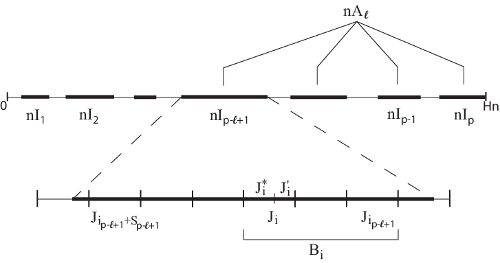
Refer to caption
Figure 1. Notation

We have,

|μ(M(Bi∪n\displaystyle|\mu(M(B_{i}\cup n Aℓ−1)≤un)−(1−rnμ(X>un))μ(M(Bi−1∪nAℓ−1)≤un)|\displaystyle A_{\ell-1})\leq u_{n})-(1-r_{n}\mu(X>u_{n}))\mu(M(B_{i-1}\cup nA_{\ell-1})\leq u_{n})|
=|μ⁡(M⁡(Bi∪n​Aℓ−1)≤un)−μ⁡(M⁡(Bi−1∪n​Aℓ−1)≤un)\displaystyle=\Big|\mu(M(B_{i}\cup nA_{\ell-1})\leq u_{n})-\mu(M(B_{i-1}\cup nA_{\ell-1})\leq u_{n})
+rnμ(X>un)μ(M(Bi−1∪nAℓ−1)≤un)|\displaystyle\qquad\qquad\quad+r_{n}\mu(X>u_{n})\mu(M(B_{i-1}\cup nA_{\ell-1})\leq u_{n})\Big|
≤|μ⁡(M⁡(Bi∪n​Aℓ−1)≤un)−μ⁡(M⁡(Bi−1∪n​Aℓ−1)≤un)\displaystyle\leq\Big|\mu(M(B_{i}\cup nA_{\ell-1})\leq u_{n})-\mu(M(B_{i-1}\cup nA_{\ell-1})\leq u_{n})
+(rn−tn)μ(X>un)μ(M(Bi−1∪nAℓ−1)≤un)|\displaystyle\qquad\qquad\quad+(r_{n}-t_{n})\mu(X>u_{n})\mu(M(B_{i-1}\cup nA_{\ell-1})\leq u_{n})\Big|
+tn​μ​(X>un)​μ​(M⁡(Bi−1∪n​Aℓ−1)≤un)\displaystyle\quad+t_{n}\mu(X>u_{n})\mu(M(B_{i-1}\cup nA_{\ell-1})\leq u_{n})
≤|μ⁡(M⁡(Bi∪n​Aℓ−1)≤un)−μ⁡(M⁡(Bi−1∪n​Aℓ−1)≤un)\displaystyle\leq\Big|\mu(M(B_{i}\cup nA_{\ell-1})\leq u_{n})-\mu(M(B_{i-1}\cup nA_{\ell-1})\leq u_{n})
+∑j=0rn−tn−1μ({Xj+H​n−i​rn>un}∩{M(Bi∪nAℓ−1)≤un)}|\displaystyle\qquad\qquad\quad+\sum_{j=0}^{r_{n}-t_{n}-1}\mu(\{X_{j+Hn-ir_{n}}>u_{n}\}\cap\{M(B_{i}\cup nA_{\ell-1})\leq u_{n})\}\Big|
+|(rn−tn)​μ​(X>un)​μ​(M⁡(Bi−1∪n​Aℓ−1)≤un)\displaystyle\quad+\Big|(r_{n}-t_{n})\mu(X>u_{n})\mu(M(B_{i-1}\cup nA_{\ell-1})\leq u_{n})
−∑j=0rn−tn−1μ({Xj+H​n−i​rn>un}∩{M(Bi∪nAℓ−1)≤un)}|\displaystyle\qquad\qquad\quad-\sum_{j=0}^{r_{n}-t_{n}-1}\mu(\{X_{j+Hn-ir_{n}}>u_{n}\}\cap\{M(B_{i}\cup nA_{\ell-1})\leq u_{n})\}\Big|
+tn​μ​(X>un).\displaystyle\quad+t_{n}\mu(X>u_{n}).

By Lemma 4.2, we obtain

|μ(M(Bi∪n\displaystyle\Big|\mu(M(B_{i}\cup n Aℓ−1)≤un)−(1−rnμ(X>un))μ(M(Bi−1∪nAℓ−1)≤un)|\displaystyle A_{\ell-1})\leq u_{n})-(1-r_{n}\mu(X>u_{n}))\mu\left(M(B_{i-1}\cup nA_{\ell-1})\leq u_{n}\right)\Big|
≤2(rn−tn)∑j=1rn−tn−1μ({X>un}∩{Xj>un})+tnμ(X>un)\displaystyle\leq 2(r_{n}-t_{n})\sum_{j=1}^{r_{n}-t_{n}-1}\mu(\{X>u_{n}\}\cap\{X_{j}>u_{n}\})+t_{n}\mu(X>u_{n})
+∑j=0rn−tn−1|μ(X>un)μ(M(Bi−1∪nAℓ−1)≤un)\displaystyle\quad+\sum_{j=0}^{r_{n}-t_{n}-1}\Big|\mu(X>u_{n})\mu(M(B_{i-1}\cup nA_{\ell-1})\leq u_{n})
−μ({X>un}∩{M((Bi−1∪nAℓ−1)−dj)≤un})|\displaystyle\qquad\qquad\quad-\mu(\{X>u_{n}\}\cap\{M((B_{i-1}\cup nA_{\ell-1})-d_{j})\leq u_{n}\})\Big|
+tn​μ​(X>un),\displaystyle\quad+t_{n}\mu(X>u_{n}),

where dj=(j+H​n−i​rn)d_{j}=(j+Hn-ir_{n}). Now using condition D3​(un)D_{3}(u_{n}), we obtain

|μ⁡(M⁡(Bi∪n​Aℓ−1)≤un)−(1−rn​μ​(X>un))​μ​(M⁡(Bi−1∪n​Aℓ−1)≤un)|≤2(rn−tn)∑j=1rn−tn−1μ({X>un}∩{Xj>un})+2tnμ(X>un)+(rn−tn)γ(n,tn).\Big|\mu(M(B_{i}\cup nA_{\ell-1})\leq u_{n})-(1-r_{n}\mu(X>u_{n}))\mu(M(B_{i-1}\cup nA_{\ell-1})\leq u_{n})\Big|\\ \leq 2(r_{n}-t_{n})\sum_{j=1}^{r_{n}-t_{n}-1}\mu(\{X>u_{n}\}\cap\{X_{j}>u_{n}\})+2t_{n}\mu(X>u_{n})+(r_{n}-t_{n})\gamma(n,t_{n}).

Set

Υk,n:=2(rn−tn)∑j=1rn−tn−1μ({X>un}∩{Xj>un})+2tnμ(X>un)+(rn−tn)γ(n,tn).\Upsilon_{k,n}:=2(r_{n}-t_{n})\sum_{j=1}^{r_{n}-t_{n}-1}\mu(\{X>u_{n}\}\cap\{X_{j}>u_{n}\})+2t_{n}\mu(X>u_{n})+(r_{n}-t_{n})\gamma(n,t_{n}).

Recalling (1.4), we may assume that nn and kk are sufficiently large so that nk​μ​(X>un)<2\frac{n}{k}\mu(X>u_{n})<2 and |1−rn​μ​(X>un)|<1|1-r_{n}\mu(X>u_{n})|<1 which implies

|μ⁡(M⁡(BSp−ℓ+1∪n​Aℓ−1)≤un)−(1−rn​μ​(X>un))​μ​(M⁡(BSp−ℓ+1−1∪n​Aℓ−1)≤un)|≤Υk,n,\displaystyle\left|\mu(M(B_{S_{p-\ell+1}}\cup nA_{\ell-1})\leq u_{n})-(1-r_{n}\mu(X>u_{n}))\mu(M(B_{S_{p-\ell+1}-1}\cup nA_{\ell-1})\leq u_{n})\right|\leq\Upsilon_{k,n},

and

|μ⁡(M⁡(BSp−ℓ+1∪n​Aℓ−1)≤un)−(1−rn​μ​(X>un))2​μ​(M⁡(BSp−ℓ+1−2∪n​Aℓ−1)≤un)|\displaystyle\left|\mu(M(B_{S_{p-\ell+1}}\cup nA_{\ell-1})\leq u_{n})-(1-r_{n}\mu(X>u_{n}))^{2}\mu(M(B_{S_{p-\ell+1}-2}\cup nA_{\ell-1})\leq u_{n})\right|
≤|μ⁡(M⁡(BSp−ℓ+1∪n​Aℓ−1)≤un)−(1−rn​μ​(X>un))​μ​(M⁡(BSp−ℓ+1−1∪n​Aℓ−1)≤un)|\displaystyle\leq\Big|\mu(M(B_{S_{p-\ell+1}}\cup nA_{\ell-1})\leq u_{n})-(1-r_{n}\mu(X>u_{n}))\mu(M(B_{S_{p-\ell+1}-1}\cup nA_{\ell-1})\leq u_{n})\Big|
+|1−rn​μ​(X>un)||μ⁡(M⁡(BSp−ℓ+1−1∪n​Aℓ−1)≤un)\displaystyle\quad+\left|1-r_{n}\mu(X>u_{n})\right|\Big|\mu(M(B_{S_{p-\ell+1}-1}\cup nA_{\ell-1})\leq u_{n})
−(1−rnμ(X>un))μ(M(BSp−ℓ+1−2∪nAℓ−1)|\displaystyle\hskip 199.16928pt-(1-r_{n}\mu(X>u_{n}))\mu(M(B_{S_{p-\ell+1}-2}\cup nA_{\ell-1})\Big|
≤2​Υk,n.\displaystyle\leq 2\Upsilon_{k,n}.

Inductively, we obtain

|μ⁡(M⁡(BSp−l+1∪n​Aℓ−1)≤un)−(1−rn​μ​(X>un))Sp−ℓ+1​μ​(M⁡(n​Aℓ−1)≤un)|≤Sp−ℓ+1​Υk,n.\displaystyle\left|\mu(M(B_{S_{p-l+1}}\cup nA_{\ell-1})\leq u_{n})-(1-r_{n}\mu(X>u_{n}))^{S_{p-\ell+1}}\mu(M(nA_{\ell-1})\leq u_{n})\right|\leq S_{p-\ell+1}\Upsilon_{k,n}.

Using Lemma 4.2,

|μ⁡(M⁡(n​Aℓ)≤un)−(1−rn​μ​(X>un))Sp−ℓ+1​μ​(M⁡(n​Aℓ−1)≤un)|\displaystyle\left|\mu(M(nA_{\ell})\leq u_{n})-(1-r_{n}\mu(X>u_{n}))^{S_{p-\ell+1}}\mu(M(nA_{\ell-1})\leq u_{n})\right|
≤|μ⁡(M⁡(n​Aℓ)≤un)−μ⁡(M⁡(BSp−l+1∪n​Aℓ−1)≤un)|\displaystyle\leq\left|\mu(M(nA_{\ell})\leq u_{n})-\mu(M(B_{S_{p-l+1}}\cup nA_{\ell-1})\leq u_{n})\right|
+|μ⁡(M⁡(BSp−l+1∪n​Aℓ−1)≤un)−(1−rn​μ​(X>un))Sp−ℓ+1​μ​(M⁡(n​Aℓ−1)≤un)|\displaystyle\hskip 56.9055pt+\left|\mu(M(B_{S_{p-l+1}}\cup nA_{\ell-1})\leq u_{n})-(1-r_{n}\mu(X>u_{n}))^{S_{p-\ell+1}}\mu(M(nA_{\ell-1})\leq u_{n})\right|
≤|μ(M(nIp−ℓ+1∪nAℓ−1)≤un)−μ(M(∪i=iℓSp−ℓ+1Ji∪nAℓ−1)≤un)|+Sp−l+1Υk,n\displaystyle\leq\left|\mu(M(nI_{p-\ell+1}\cup nA_{\ell-1})\leq u_{n})-\mu(M(\cup_{i=i_{\ell}}^{S_{p-\ell+1}}J_{i}\cup nA_{\ell-1})\leq u_{n})\right|+S_{p-l+1}\Upsilon_{k,n}
≤2​rn​μ​(X>un)+Sp−l+1​Υk,n.\displaystyle\leq 2r_{n}\mu(X>u_{n})+S_{p-l+1}\Upsilon_{k,n}.

In the next step we have

|μ⁡(M⁡(n​Aℓ)≤un)−(1−rn​μ​(X>un))Sp−ℓ+1+Sp−ℓ+2​μ​(M⁡(n​Aℓ−2)≤un)|\displaystyle\Big|\mu(M(nA_{\ell})\leq u_{n})-(1-r_{n}\mu(X>u_{n}))^{S_{p-\ell+1}+S_{p-\ell+2}}\mu(M(nA_{\ell-2})\leq u_{n})\Big|
≤|μ⁡(M⁡(n​Aℓ)≤un)−(1−rn​μ​(X>un))Sp−ℓ+1​μ​(M⁡(n​Aℓ−1)≤un)|\displaystyle\leq\Big|\mu(M(nA_{\ell})\leq u_{n})-(1-r_{n}\mu(X>u_{n}))^{S_{p-\ell+1}}\mu(M(nA_{\ell-1})\leq u_{n})\Big|
+|1−rn​μ​(X>un)|Sp−ℓ+1|μ⁡(M⁡(n​Aℓ−1)≤un)\displaystyle\hskip 28.45274pt+\left|1-r_{n}\mu(X>u_{n})\right|^{S_{p-\ell+1}}\Big|\mu(M(nA_{\ell-1})\leq u_{n})
−(1−rnμ(X>un))Sp−ℓ+2μ(M(nAℓ−2)≤un)|\displaystyle\hskip 199.16928pt-(1-r_{n}\mu(X>u_{n}))^{S_{p-\ell+2}}\mu(M(nA_{\ell-2})\leq u_{n})\Big|
≤4​rn​μ​(X>un)+(Sp−ℓ+1+Sp−ℓ+2)​Υk,n.\displaystyle\leq 4r_{n}\mu(X>u_{n})+(S_{p-\ell+1}+S_{p-\ell+2})\Upsilon_{k,n}.

Therefore, by induction, we obtain

|μ⁡(M⁡(n​Ap)≤un)−(1−rn​μ​(X>un))∑j=1pSj|≤2​p​rn​μ​(X>un)+∑j=1pSj​Υk,n.\displaystyle\left|\mu(M(nA_{p})\leq u_{n})-(1-r_{n}\mu(X>u_{n}))^{\sum_{j=1}^{p}S_{j}}\right|\leq 2pr_{n}\mu(X>u_{n})+{\sum_{j=1}^{p}S_{j}}\Upsilon_{k,n}.

Now, it is easy to see that Sj∼k​|Ij|S_{j}\sim k|I_{j}|, for each j∈{1,…,p}j\in\{1,\ldots,p\}. Consequently,

limk→+∞limn→+∞(1−rn​μ​(X>un))∑j=1pSj=limk→+∞limn→+∞(1−⌊nk⌋​μ​(X>un))∑j=1pSj\displaystyle\lim_{k\rightarrow+\infty}\lim_{n\rightarrow+\infty}\left(1-r_{n}\mu(X>u_{n})\right)^{{\sum_{j=1}^{p}}S_{j}}=\lim_{k\rightarrow+\infty}\lim_{n\rightarrow+\infty}\left(1-\left\lfloor\frac{n}{k}\right\rfloor\mu(X>u_{n})\right)^{{\sum_{j=1}^{p}}S_{j}}
=limk→+∞(1−τk)∑j=1pSj=limk→+∞[(1−τk)k​∑j=1p|Ij|]∑j=1pSjk​∑j=1p|Ij|=e−τ∑j=1p|Ij|\displaystyle=\lim_{k\rightarrow+\infty}\left(1-\frac{\tau}{k}\right)^{{\sum_{j=1}^{p}}S_{j}}=\lim_{k\rightarrow+\infty}\left[\left(1-\frac{\tau}{k}\right)^{k\sum_{j=1}^{p}|I_{j}|}\right]^{\frac{{\sum_{j=1}^{p}}S_{j}}{k\sum_{j=1}^{p}|I_{j}|}}=\text{e}^{-\tau\sum_{j=1}^{p}|I_{j}|}
=∏j=1pe−τ⁡(bj−aj).\displaystyle=\prod_{j=1}^{p}\text{e}^{-\tau(b_{j}-a_{j})}.

To conclude the proof it suffices to show that

limk→+∞limn→+∞(2​p​rn​μ​(X>un)+k​H​Υk,n)=0.\lim_{k\rightarrow+\infty}\lim_{n\rightarrow+\infty}(2pr_{n}\mu(X>u_{n})+kH\Upsilon_{k,n})=0.

We start by noting that, since n​μ​(X>un)→τ≥0n\mu(X>u_{n})\to\tau\geq 0,

limk→+∞limn→+∞2​p​rn​μ​(X>un)=limk→+∞2​p​τk=0.\lim_{k\rightarrow+\infty}\lim_{n\rightarrow+\infty}2pr_{n}\mu(X>u_{n})=\lim_{k\rightarrow+\infty}\frac{2p\tau}{k}=0.

Next we need to check that

limk→+∞limn→+∞k​Υk,n=0,\lim_{k\rightarrow+\infty}\lim_{n\rightarrow+\infty}k\Upsilon_{k,n}=0,

which means,

limk→+∞limn→+∞2k(rn−tn)∑j=1rn−tn−1μ({X>un}∩{Xj>un})+2ktnμ(X>un)+k⁡(rn−tn)​γ​(n,tn)=0.\lim_{k\rightarrow+\infty}\lim_{n\rightarrow+\infty}2k(r_{n}-t_{n})\sum_{j=1}^{r_{n}-t_{n}-1}\mu(\{X>u_{n}\}\cap\{X_{j}>u_{n}\})+2kt_{n}\mu(X>u_{n})\\ +k(r_{n}-t_{n})\gamma(n,t_{n})=0.

Assume that t=tnt=t_{n} where tn=o⁡(n)t_{n}=o(n) is given by Condition D3​(un)D_{3}(u_{n}). Now, observe that, by (1.4), for every k∈ℕk\in\mathbb{N}, we have limn→∞k​tn​μ​(X>un)=0\lim_{n\to\infty}kt_{n}\mu(X>u_{n})=0. Finally, use D3​(un)D_{3}(u_{n}) and D′​(un)D^{\prime}(u_{n}) to prove that the two remaining terms also go to 00. ∎

Proof of Theorem 5.

Since the Poisson Process has no fixed atoms, that is, points tt such that μ⁡(N⁡({t})>0)>0\mu\left(N(\{t\})>0\right)>0, the convergence is equivalent to convergence of finite dimensional distributions. But, because NN is a simple point process, without multiple events, we may use a criterion proposed by Kallenberg [Ka, Theorem 4.7] to show the stated convergence. Namely we need to verify that

  1. (1)

    𝔼⁡(Nn​(I))→n→∞𝔼⁡(N⁡(I))\mathbb{E}(N_{n}(I))\xrightarrow[n\to\infty]{}\mathbb{E}(N(I)), for all I∈𝒮I\in\mathcal{S};

  2. (2)

    μ⁡(Nn​(A)=0)→n→∞μ⁡(N⁡(A)=0)\mu(N_{n}(A)=0)\xrightarrow[n\to\infty]{}\mu(N(A)=0), for all A∈ℛA\in\mathcal{R},

where 𝔼⁡(⋅)\mathbb{E}(\cdot) denotes the expectation with respect to μ\mu.

First we show that condition (1) holds. Let a,b∈ℝ+a,b\in\mathbb{R}^{+} be such that I=[a,b)I=[a,b), then, recalling that vn=1/μ⁡(X0>un)v_{n}=1/\mu(X_{0}>u_{n}), we have

𝔼​(Nn​(I))\displaystyle\mathbb{E}(N_{n}(I)) =𝔼(∑j=⌊vn​a⌋+1⌊vn​b⌋𝟏{Xj>un})=∑j=⌊vn​a⌋+1⌊vn​b⌋E(𝟏{Xj>un})\displaystyle=\mathbb{E}\left(\sum_{j=\lfloor v_{n}a\rfloor+1}^{\lfloor v_{n}b\rfloor}{\bf 1}_{\{X_{j}>u_{n}\}}\right)=\sum_{j=\lfloor v_{n}a\rfloor+1}^{\lfloor v_{n}b\rfloor}E({\bf 1}_{\{X_{j}>u_{n}\}})
=(⌊vn​b⌋−(⌊vn​a⌋+1))​μ​(X0>un)\displaystyle=\left(\lfloor v_{n}b\rfloor-(\lfloor v_{n}a\rfloor+1)\right)\mu(X_{0}>u_{n})
∼(b−a)​vn​μ​(X0>un)→n→∞(b−a)=𝔼⁡(N⁡(I)).\displaystyle\sim(b-a)v_{n}\mu(X_{0}>u_{n})\xrightarrow[n\to\infty]{}(b-a)=\mathbb{E}(N(I)).

To prove condition (2), let s∈ℕs\in\mathbb{N} and A=∪i=1sIiA=\cup_{i=1}^{s}I_{i} where I1,…,Is∈𝒮I_{1},\ldots,I_{s}\in\mathcal{S} are disjoint. Also let aj,bj∈ℝ+a_{j},b_{j}\in\mathbb{R}^{+} be such that Ij=[aj,bj)I_{j}=[a_{j},b_{j}). By Proposition 1, we have

μ(Nn(A)=0)=μ(∩i=1s{M(vnIj)≤un})∼μ(∩i=1s{M((n/τ)Ij)≤un})→n→∞∏j=1se−(bj−aj).\mu(N_{n}(A)=0)=\mu\left(\cap_{i=1}^{s}\{M(v_{n}I_{j})\leq u_{n}\}\right)\sim\mu\left(\cap_{i=1}^{s}\{M((n/\tau)I_{j})\leq u_{n}\}\right)\xrightarrow[n\to\infty]{}\prod_{j=1}^{s}\text{e}^{-(b_{j}-a_{j})}.

The result follows at once since μ⁡(N⁡(A)=0)=∏i=1sμ⁡(N⁡(Ij)=0)=∏j=1se−(bj−aj)\mu(N(A)=0)=\prod_{i=1}^{s}\mu(N(I_{j})=0)=\prod_{j=1}^{s}\text{e}^{-(b_{j}-a_{j})}. ∎

Proof of Corollary 6.

In [FF1, FF2], conditions D2​(un)D_{2}(u_{n}) and D′​(un)D^{\prime}(u_{n}) were proved for stochastic processes X0,X1,…X_{0},X_{1},\ldots as in (1.1) and (1.9) with ζ\zeta being either the critical point or the critical value and observables of type g3g_{3} (g3​(x)=xg_{3}(x)=x for ζ=1\zeta=1 and g3=1−a​x2g_{3}=1-ax^{2} for ζ=0\zeta=0).

Observe that independently of the type of gg, the sequence unu_{n} is computed so that an exceedance of the level unu_{n} corresponds to a visit to the ball Bδn​(ζ)B_{\delta_{n}}(\zeta), where δn\delta_{n} is such that μ⁡(Bδn)∼τ/n\mu(B_{\delta_{n}})\sim\tau/n. This means that condition D′​(un)D^{\prime}(u_{n}) can be written in terms of returns to Bδn​(ζ)B_{\delta_{n}}(\zeta) which implies that it holds for every sequence X0,X1,…X_{0},X_{1},\ldots, independently of the shape of gg.

Condition D3​(un)D_{3}(u_{n}) follows from decay of correlations. In fact, from [KN, Y1] one has that for all ϕ,ψ:M→ℝ\phi,\psi:M\rightarrow\mathbb{R} with bounded variation, there is C,α>0C,\alpha>0 independent of ϕ,ψ\phi,\psi and nn such that

|∫ϕ⋅(ψ∘ft)​𝑑μ−∫ϕ​𝑑μ​∫ψ​𝑑μ|≤C​Var​(ϕ)​‖ψ‖∞​e−α​t,∀t∈ℕ0,\left|\int\phi\cdot(\psi\circ f^{t})d\mu-\int\phi d\mu\int\psi d\mu\right|\leq C\mbox{Var}(\phi)\|\psi\|_{\infty}\text{e}^{-\alpha t},\quad\forall t\in\mathbb{N}_{0}, (4.4)

where Var​(ϕ)\mbox{Var}(\phi) denotes the total variation of ϕ\phi. For each A∈ℛA\in\mathcal{R}, take ϕ=𝟏{X0>un}\phi={\bf 1}_{\{X_{0}>u_{n}\}} and ψ=𝟏{M(A)≤un}\psi={\bf 1}_{\{M(A)\leq u_{n}\}}, then (4.4) implies that Condition D3​(un)D_{3}(u_{n}) holds with γ⁡(n,t)=γ⁡(t):=2​C​e−α​t\gamma(n,t)=\gamma(t):=2C\text{e}^{-\alpha t} and for the sequence tn=nt_{n}=\sqrt{n}, for example. ∎

5. Poisson Statistics for first return times

The purpose of this section is to discuss what is known about the Poisson statistics of first return times to balls. The main focus is on showing that a map f∈N​F2f\in N\!F^{2} with an acip must have the RTPP asymptotically converging to a Poisson Process. However, for more generality we will introduce the ideas assuming that our phase space 𝒳\mathcal{X} is a Riemannian manifold. We note that a similar result to the main theorem [HLV] implies that the limit laws for the HTPP and RTPP are the same. So since the results we will cite below are usually given in terms of RTS, we will use this.

Similarly to the proof of Theorem 5, in order to show that the RTPP has a Poisson limit, it suffices to prove that for k∈ℕk\in\mathbb{N} and a rectangle Rk⊂ℝkR_{k}\subset\mathbb{R}^{k},

|μUn​((wUn,wUn2,…,wUnk)∈1μ⁡(Un)​Rk)−∫RkΠi=1k​eti​d​tk|→0​ as ​n→∞.\left|\mu_{U_{n}}\left((w_{U_{n}},w_{U_{n}}^{2},\ldots,w_{U_{n}}^{k})\in\frac{1}{\mu(U_{n})}R_{k}\right)-\int_{R_{k}}\Pi_{i=1}^{k}\text{e}^{t_{i}}~dt^{k}\right|\to 0\text{ as }n\to\infty.

The main result of [BSTV] is that the RTS for an inducing scheme is the same for the inducing scheme as for the original system. However, they remark in that paper that their methods extend to give the same Poisson statistics for the inducing scheme and the original system. In [BT], the theory in [BSTV] was extended to show that for multimodal maps of the interval the RTS of suitable inducing schemes converge to the RTS of the original system. The corresponding result for Poisson statistics follows similarly. For multimodal maps f:I→If:I\to I, with an acip μ\mu, those inducing schemes are Rychlik maps. Therefore to prove that the original (I,f,μ)(I,f,\mu) has the RTPP converging to a Poisson process, we must show that the induced, Rychlik, maps also have this property. As we sketch below, this can be proved using [HSV, Theorem 2.6].

For a system (X,F,μ)(X,F,\mu), we say that a partition 𝒬{\mathcal{Q}} is uniform mixing if there exists γ𝒬​(n)→0\gamma_{\mathcal{Q}}(n)\to 0 as n→∞n\to\infty, such that

γ𝒬​(n):=supk,lsupB∈F−(n+k)​σ​𝒬lA∈σ​𝒬k|μ⁡(A∩B)−μ⁡(A)​μ​(B)|.\gamma_{\mathcal{Q}}(n):=\sup_{k,l}\sup_{\stackrel{{\scriptstyle A\in\sigma{\mathcal{Q}}_{k}}}{{B\in F^{-(n+k)}\sigma{\mathcal{Q}}_{l}}}}\left|\mu(A\cap B)-\mu(A)\mu(B)\right|.

Here 𝒬k:=⋁j=0k−1F−j​𝒬{\mathcal{Q}}_{k}:=\bigvee_{j=0}^{k-1}F^{-j}{\mathcal{Q}} and σ​𝒬k\sigma{\mathcal{Q}}_{k} is the sigma algebra generated by 𝒬k{\mathcal{Q}}_{k}. For our purposes 𝒬{\mathcal{Q}} will be {U,Uc}\{U,U^{c}\} where UU is a ball around ζ\zeta.

By [HSV, Theorem 2.6], if we assume the system is uniform mixing for {U,Uc}\{U,U^{c}\}, then for a rectangle Rk⊂ℝkR_{k}\subset\mathbb{R}^{k},

|μU​((wU,wU2,…,wUk)∈1μ⁡(U)​Rk)−∫RkΠi=1k​eti​d​tk|≤E​r​r​(k,U).\left|\mu_{U}\left((w_{U},w_{U}^{2},\ldots,w_{U}^{k})\in\frac{1}{\mu(U)}R_{k}\right)-\int_{R_{k}}\Pi_{i=1}^{k}\text{e}^{t_{i}}~dt^{k}\right|\leq Err(k,U). (5.1)

Moreover, the term E​r​r​(k,U)Err(k,U) goes to 0 as UU shrinks to a point ζ\zeta. In fact, we have E​r​r​(k,U)=k⁡(3​d​(U)+R⁡(k,U))Err(k,U)=k\left(3d(U)+R(k,U)\right) where R⁡(k,U)→0R(k,U)\to 0 as μ⁡(U)→0\mu(U)\to 0 and the rate that R⁡(k,U)R(k,U) goes to zero depends on how γ𝒬\gamma_{\mathcal{Q}} shrinks with UU . As was shown in [BSTV], for Rychlik maps the quantity d⁡(U)d(U) tends 0 as U→{ζ}U\to\{\zeta\}. Therefore it only remains to show that the Rychlik maps defined in [BT] are uniform mixing for {U,Uc}\{U,U^{c}\}.

Since we assumed that (X,F,μ)(X,F,\mu) is Rychlik, [R, Theorem 5] implies that the natural partition 𝒫1\mathcal{P}_{1}, consisting of maximal intervals on which ff is a homeomorphism, is Bernoulli, with exponential speed. Since (X,F,μ)(X,F,\mu) is uniformly expanding, this implies that {U,Uc}\{U,U^{c}\} is also Bernoulli, with exponential speed. As noted in [HSV, Remark 2.5], this implies that {U,Uc}\{U,U^{c}\} is uniform mixing, as required.

The proof that the successive returns form a point process converging to a Poisson Process follows from (5.1) and the Kallenberg argument used in the proof of Theorem 5.

6. EVL and HTS in higher dimensions

In this section, we extend Collet’s theory of maps with exponential decay of correlations from one dimension to higher dimensions. We conclude with an example.

Let 𝒳\mathcal{X} be as usual a dd-dimensional compact Riemannian manifold and f:𝒳→𝒳f:\mathcal{X}\to\mathcal{X} a C2C^{2} endomorphism. We say that ff admits a Young tower if there exists a ball Δ⊂𝒳\Delta\subset\mathcal{X}, a countable partition 𝒫\mathcal{P} (mod 0) of Δ\Delta into topological balls Δi\Delta_{i} with smooth boundaries, and a return time function R:Δ→ℕR:\Delta\to\mathbb{N} piecewise constant on elements of 𝒫\mathcal{P} satisfying the following properties:

  1. (Y1)

    Markov: for each Δi∈𝒫\Delta_{i}\in\mathcal{P} and R=R⁡(Δi)R=R(\Delta_{i}), fR:Δi→Δf^{R}:\Delta_{i}\to\Delta is a C2C^{2} diffeomorphism (and in particular a bijection). Thus the induced map

    F:Δ→Δ​ given by ​F​(x)=fR⁡(x)​(x)F:\Delta\to\Delta\ \text{ given by }\ F(x)=f^{R(x)}(x)

    is defined almost everywhere and satisfies the classical Markov property. We consider also the separation time s⁡(x,y)s(x,y) given by the maximum integer such that Fi​(x)F^{i}(x) and Fi​(y)F^{i}(y) belong to the same element of the partition 𝒫\mathcal{P} for all i≤s⁡(x,y)i\leq s(x,y), which we assume to be defined and finite for almost every pair of points x,y∈Δx,y\in\Delta.

  2. (Y2)

    Uniform backward contraction: There exist C>0C>0 and 0<β<10<\beta<1 such that for x,y∈Δx,y\in\Delta and any 0≤n≤s⁡(x,y)0\leq n\leq s(x,y) we have

    dist​(fn​(x),fn​(y))≤C​βs⁡(x,y)−n.\mbox{dist}(f^{n}(x),f^{n}(y))\leq C\beta^{s(x,y)-n}.
  3. (Y3)

    Bounded distortion: For any x,y∈Δx,y\in\Delta and any 0≤k≤n<s⁡(x,y)0\leq k\leq n<s(x,y) we have

    log∏i=kndetD​f​(fi​(x))detD​f​(fi​(x))≤Cβs⁡(x,y)−n\log\prod_{i=k}^{n}\frac{\det Df(f^{i}(x))}{\det Df(f^{i}(x))}\leq C\beta^{s(x,y)-n}
  4. (Y4)

    Integrable return times:

    ∫R​𝑑Leb<∞\int R\;d{\rm Leb}<\infty

In this section we only consider maps admitting a Young tower with exponential return time tail which means that we will replace condition (Y4) by the following stronger one

  1. (Y4’)

    Exponential tail decay: There is C,α>0C,\alpha>0 such that

    Leb({R>n})=Ce−α​n.{\rm Leb}(\{R>n\})=C\text{e}^{-\alpha n}.

These systems have been studied, in a more general context, by L.S. Young in [Y2, Y3], where several examples can also be found. Among the properties proved by L.S. Young we mention the existence of an FF-invariant measure μ0\mu_{0} that is equivalent to Lebesgue measure on Δ\Delta (meaning that its density is bounded above and below by a constant). After saturating one gets an absolutely continuous (w.r.t. Lebesgue), ff-invariant probability given by

μ(A)=R¯−1∑ℓ=0∞μ0(f−ℓ(A)∩{R>ℓ}),\mu(A)=\bar{R}^{-1}\sum_{\ell=0}^{\infty}\mu_{0}\left(f^{-\ell}(A)\cap\{R>\ell\}\right), (6.1)

where R¯=∫ΔR​d​μ0\bar{R}=\int_{\Delta}Rd\mu_{0}. One of the main achievements in [Y2, Y3] is the fact that the decay of the tail of return times determines the speed of decay of correlations for Hölder continuous (or Lipschitz) observables. Namely, if ϕ:𝒳→ℝ\phi:\mathcal{X}\to\mathbb{R} is Hölder continuous of exponent 0<ι≤10<\iota\leq 1, with Hölder constant

Kι​(ϕ):=supx≠y|ϕ⁡(x)−ϕ⁡(y)|(dist​(x,y))ι,K_{\iota}(\phi):=\sup_{x\neq y}\frac{|\phi(x)-\phi(y)|}{\left(\mbox{dist}(x,y)\right)^{\iota}},

ψ:𝒳→ℝ\psi:\mathcal{X}\to\mathbb{R} is in L∞​(Leb)L^{\infty}({\rm Leb}) and the tower has exponential tail, then there are C>0C>0 and α′>0\alpha^{\prime}>0 such that

|∫ϕ⋅(ψ∘ft)​𝑑μ−∫ϕ​𝑑μ​∫ψ​𝑑μ|≤C​Kι​(ϕ)​‖ψ‖∞​e−α​t,∀t∈ℕ0.\left|\int\phi\cdot(\psi\circ f^{t})d\mu-\int\phi d\mu\int\psi d\mu\right|\leq CK_{\iota}(\phi)\|\psi\|_{\infty}\text{e}^{-\alpha t},\quad\forall t\in\mathbb{N}_{0}. (6.2)
Theorem 6.

Let 𝒳\mathcal{X} be a dd-dimensional compact Riemannian manifold and assume that f:𝒳→𝒳f:\mathcal{X}\to\mathcal{X} is a C2C^{2} endomorphism admitting a Young tower with exponential tail. Consider a stochastic process X0,X1,…X_{0},X_{1},\ldots defined by (1.1) and (1.9), for some choice of ζ∈𝒳\zeta\in\mathcal{X}. Then, for Leb{\rm Leb}-almost every ζ∈𝒳\zeta\in\mathcal{X} chosen, conditions D3​(un)D_{3}(u_{n}) (or D2​(un)D_{2}(u_{n})) and D′​(un)D^{\prime}(u_{n}) hold, where unu_{n} is a sequence of levels satisfying (1.4).

Together with the results in Section 1.3, Section 3 and Section 4 we get the following corollary.

Corollary 7.

Let 𝒳\mathcal{X} be a dd-dimensional compact Riemannian manifold and assume that f:𝒳→𝒳f:\mathcal{X}\to\mathcal{X} is a C2C^{2} endomorphism admitting a Young tower with exponential tail. Consider a stochastic process X0,X1,…X_{0},X_{1},\ldots defined by (1.1) and (1.9) for some ζ∈𝒳\zeta\in\mathcal{X}. Then, for Leb{\rm Leb}-almost every choice of ζ∈𝒳\zeta\in\mathcal{X}, the following assertions hold:

  1. (1)

    We have an EVL for MnM_{n}, defined in (1.2), which coincides with that one of M^n\hat{M}_{n} defined in (1.5). In particular, it must be of one of the three classical types. Moreover, for every i∈{1,2,3}i\in\{1,2,3\}, if gg is of type gig_{i} then we have an EVL for MnM_{n} of type E​ViE\!V_{i}.

  2. (2)

    We have exponential HTS to balls at ζ∈𝒳\zeta\in\mathcal{X}.

  3. (3)

    The EPP NnN_{n} defined in (3.3) is such that Nn→𝑑NN_{n}\xrightarrow{d}N, as n→∞n\rightarrow\infty, where NN denotes a Poisson Process with intensity 11.

  4. (4)

    The same applies to the HTPP Nn∗N_{n}^{*} defined in (3.2).

6.1. Proof of Theorem 6

To show this result, one needs only to realise that Collet’s proof of [Col2, Theorem 1] may be mimicked in our multi-dimensional setting with minor adjustments. Thus, instead of repeating all the arguments, we will prove that D3​(un)D_{3}(u_{n}) and D′​(un)D^{\prime}(u_{n}) hold just by redoing the parts that need to be adapted to this more general higher dimensional setting. However, in order to keep on track we will restate all the Lemmas (with the necessary adjustments) of Collet’s proof.

The first lemma is technical and very simple to prove.

Lemma 6.1.

For any v≥1v\geq 1

∑l,Rl>vRl​Leb​(Δl)≤{2∑s=v/2∞Leb({R>s}),∑s=v∞Leb({R>s})+vLeb({R>v}).\sum_{l,\,R_{l}>v}R_{l}\;{\rm Leb}(\Delta_{l})\leq\begin{cases}2\sum_{s=v/2}^{\infty}\;{\rm Leb}(\{R>s\})\;,&\\ \sum_{s=v}^{\infty}\;{\rm Leb}(\{R>s\})+v\,{\rm Leb}(\{R>v\})\;.&\end{cases}

See [Col2, Lemma 2.1].

Next result gives a relation between the measure μ\mu of small sets and their respective Lebesgue measure.

Lemma 6.2.

Under (Y4’), there are two positive constants CC and θ\theta such that for any Lebesgue measurable set AA, we have

μ⁡(A)≤C​Leb​(A)θ.\mu(A)\leq C{\rm Leb}(A)^{\theta}.

See [Col2, Lemma 2.2].

To prove condition D′​(un)D^{\prime}(u_{n}) we need to show that the μ\mu-measure of the set of points xx that are too rapidly recurrent is small. For every v∈ℕv\in\mathbb{N} and any ϵ>0\epsilon>0 we define the set ℰv​(ϵ){\mathcal{E}}_{v}(\epsilon) of points that come back very close to the initial position after vv iterates

ℰv​(ϵ)={x,|x−fv​(x)|<ϵ}.{\mathcal{E}}_{v}(\epsilon)=\{x\,,\,|x-f^{v}(x)|<\epsilon\}\;.

Since 𝒳\mathcal{X} is compact and ff is C2C^{2} we may define Υ:=sup{∥Df(x)∥∞x∈𝒳}\Upsilon:=\sup\{\|Df(x)\|_{\infty}\>\;x\in\mathcal{X}\}.

Proposition 6.3.

Under (Y4’), there exist positive constants CC, α′\alpha^{\prime} and η<1\eta<1 such that for any integer vv and any ϵ>0\epsilon>0 we have

μ⁡(ℰv​(ϵ))≤C⁡(v2​ϵη+e−α′​v).\mu({\mathcal{E}}_{v}(\epsilon))\leq C\left(v^{2}\epsilon^{\eta}+e^{-\alpha^{\prime}v}\right).
Proof.

We follow the proof of the corresponding result [Col2, Proposition 2.3] very closely. We will consider the intersection with ℰv​(ϵ){\mathcal{E}}_{v}(\epsilon) of the various cylinders where fvf^{v} is one-to-one. From (6.1), we have to consider the intersection of these sets with fj​(Δl)f^{j}(\Delta_{l}). We will start by choosing a number 1/2>ξ>01/2>\xi>0 such that β​Υξ<1\beta\Upsilon^{\xi}<1 and assume first that Rl<ξ​vR_{l}<\xi v. If we apply fRl−jf^{R_{l}-j} on fj​(Δl)f^{j}(\Delta_{l}), we land in Δ\Delta and we have to apply fv−Rl+jf^{v-R_{l}+j} to get the image under fvf^{v}. At this point it is convenient to introduce the following construction. Let (sj)(s_{j}) be a sequence of integers. We denote by Δs1,s2,…,sr\Delta_{s_{1},s_{2},\ldots,s_{r}} the set

Δs1,s2,…,sr=Δs1∩f−Rs1​Δs2∩f−(Rs1+Rs2)​Δs3∩⋯∩f−(Rs1+⋯+Rsr−1)​Δsr.\Delta_{s_{1},s_{2},\ldots,s_{r}}=\Delta_{s_{1}}\cap f^{-R_{s_{1}}}\Delta_{s_{2}}\cap f^{-(R_{s_{1}}+R_{s_{2}})}\Delta_{s_{3}}\cap\;\cdots\;\cap f^{-(R_{s_{1}}+\,\cdots\,+R_{s_{r-1}})}\Delta_{s_{r}}\;.

In other words, this is the subset AA of Δs1\Delta_{s_{1}} which is mapped by fRs1+⋯+Rsr−1f^{R_{s_{1}}+\cdots+R_{s_{r-1}}} bijectively onto Δsr\Delta_{s_{r}} with

fRs1+⋯+Rsp​(A)⊂Δsp+1f^{R_{s_{1}}+\cdots+R_{s_{p}}}(A)\subset\Delta_{s_{p+1}}

for p=1,…,r−1p=1,\ldots,\;r-1.

For fixed vv, ll and jj, we now consider all the sets Δs1,…,sr\Delta_{s_{1},\ldots,s_{r}} with Rs1+⋯+Rsr−1+Rl−j<vR_{s_{1}}+\cdots+R_{s_{r-1}}+R_{l}-j<v and Rs1+⋯+Rsr+Rl−j≥vR_{s_{1}}+\cdots+R_{s_{r}}+R_{l}-j\geq v. Together with {R>v−1−Rl+j}\{R>v-1-R_{l}+j\}, this gives a partition of Δ\Delta. We then construct a partition of fj​(Δl)f^{j}(\Delta_{l}) by pulling back this partition by fRl−jf^{R_{l}-j}. We now consider fvf^{v} on each atom of this partition. Let

A=Al,j,s1,…,sr=fj​(Δl)∩fj−Rl​(Δs1,…,sr).A=A_{l,j,s_{1},\ldots,s_{r}}=f^{j}(\Delta_{l})\cap f^{j-R_{l}}\left(\Delta_{s_{1},\ldots,s_{r}}\right).

We first assume that Rsr<ξ​vR_{s_{r}}<\xi v and AA has a ‘large’ image under fvf^{v}, namely

|fv​(A)|≥δ,|f^{v}(A)|\geq\delta\;,

where δ\delta is a positive number to be chosen adequately later on. Let J:=Rs1+⋯+Rsr+Rl−jJ:=R_{s_{1}}+\cdots+R_{s_{r}}+R_{l}-j and B:=ℰv​(ϵ)∩AB:={{\mathcal{E}}_{v}(\epsilon)}\cap A, which we may assume to be nonempty. We argue that |fv​(B)|=O⁡(ϵd)|f^{v}(B)|=O(\epsilon^{d}). To see this, let x,y∈Ax,y\in A be such that

dist(fv(x),fv(y))=diam(fv(B)):=sup{dist(z,w):z,w∈fv(B)}.\mbox{dist}(f^{v}(x),f^{v}(y))=\mbox{diam}(f^{v}(B)):=\sup\{\mbox{dist}(z,w):\;z,w\in f^{v}(B)\}.

By (Y2), it follows that

dist​(x,y)≤C​βJ​dist​(fJ​(x),fJ​(y)).\mbox{dist}(x,y)\leq C\beta^{J}\mbox{dist}(f^{J}(x),f^{J}(y)).

Moreover, by definition of Υ\Upsilon, we also have

dist​(fv​(x),fv​(y))≥Υ−J+v​dist​(fJ​(x),fJ​(x))≥Υ−Rsr​dist​(fJ​(x),fJ​(x)).\mbox{dist}(f^{v}(x),f^{v}(y))\geq\Upsilon^{-J+v}\mbox{dist}(f^{J}(x),f^{J}(x))\geq\Upsilon^{-R_{s_{r}}}\mbox{dist}(f^{J}(x),f^{J}(x)).

Consequently, since by assumption Rsr<ξ​vR_{s_{r}}<\xi v, we have

dist​(x,y)dist​(fv​(x),fv​(y))≤C​βJ​ΥRsr≤O⁡(βv​Υξ​v)≤O⁡((β​Υξ)v).\frac{\mbox{dist}(x,y)}{\mbox{dist}(f^{v}(x),f^{v}(y))}\leq C\beta^{J}\Upsilon^{R_{s_{r}}}\leq O(\beta^{v}\Upsilon^{\xi v})\leq O(\left(\beta\Upsilon^{\xi}\right)^{v}).

Since β​Υξ<1\beta\Upsilon^{\xi}<1, by the choice of ξ\xi, then we may pick v0∈ℕv_{0}\in\mathbb{N}, only depending on ff, such that for all v≥v0v\geq v_{0} we have

dist​(x,y)≤12​dist​(fv​(x),fv​(y)).\mbox{dist}(x,y)\leq\frac{1}{2}\,\mbox{dist}(f^{v}(x),f^{v}(y)). (6.3)

Observe that for v<v0v<v_{0}, Proposition 6.3 simply holds with CC sufficiently large.

Now, assuming that x,y∈B⊂ℰv​(ϵ)x,y\in B\subset{\mathcal{E}}_{v}(\epsilon) we have

dist​(fv​(x),fv​(y))\displaystyle\mbox{dist}(f^{v}(x),f^{v}(y)) ≤dist​(fv​(x),x)+dist​(x,y)+dist​(y,fv​(y))\displaystyle\leq\mbox{dist}(f^{v}(x),x)+\mbox{dist}(x,y)+\mbox{dist}(y,f^{v}(y))
≤ϵ+12​dist​(fv​(x),fv​(y))+ϵ.\displaystyle\leq\epsilon+\frac{1}{2}\,\mbox{dist}(f^{v}(x),f^{v}(y))+\epsilon.

This means that diam​(fv​(B))≤4​ϵ\mbox{diam}(f^{v}(B))\leq 4\epsilon. If x,y∉Bx,y\notin B then we could replace them by close enough x′,y′∈Bx^{\prime},y^{\prime}\in B so that diam​(fv​(B))≤5​ϵ\mbox{diam}(f^{v}(B))\leq 5\epsilon. Hence, we have proved that |fv​(B)|=O⁡(ϵd)\left|f^{v}(B)\right|=O(\epsilon^{d}).

Using distortion, we get

|B|/|A|=O⁡(ϵd/δ),|B|/|A|=O(\epsilon^{d}/\delta),

and

|Δl∩f−j​(B)|/|Δl∩f−j​(A)|=O⁡(ϵd/δ).|\Delta_{l}\cap f^{-j}(B)|/|\Delta_{l}\cap f^{-j}(A)|=O\left(\epsilon^{d}/\delta\right).

Since μ0\mu_{0} is equivalent to the Lebesgue measure on Δ\Delta, then

μ0​(Δl∩f−j​(B))=O⁡(ϵdδ)​μ0​(Δl∩f−j​(A)).\mu_{0}(\Delta_{l}\cap f^{-j}(B))=O\left({\frac{\epsilon^{d}}{\delta}}\right)\mu_{0}(\Delta_{l}\cap f^{-j}(A)).

Next we sum over all sets AA as above, contained in fj​(Δl)f^{j}(\Delta_{l}) and such that they have ‘large’ image under fvf^{v}. Since they are disjoint we get a contribution bounded above by O⁡(ϵd/δ)​μ0​(Δl)O(\epsilon^{d}/\delta)\mu_{0}(\Delta_{l}). Summing over jj we get a bound O⁡(ϵd/δ)​Rl​μ0​(Δl)O(\epsilon^{d}/\delta)R_{l}\mu_{0}(\Delta_{l}). Finally, summing over ll we get the estimate: O⁡(ϵd/δ)O(\epsilon^{d}/\delta). This ends the estimate in the good case when segments AA reach ‘large’ scale in vv steps.

We next have to gather the estimates for all the left-over bad cases. These bad cases are dealt with by realising that they correspond to large values of RR, whose tail we are assuming to decay exponentially fast. We skip the study of these cases and refer the reader to [Col2, Proposition 2.3] where they are treated without any particular unidimensional argument.

Finally, collecting all the estimates, there exists C>0C>0 so that

μ⁡(ℰv​(ϵ))=O⁡(ϵdδ+∑s>ξ​v/2μ0​(R>s)CLOSEOPEN+v​Leb​(R≥(1−ξ)​v)+v2​μ​(R≥ξ​v)+v2​μ​(R>C​log⁡δ−1)).\mu({{\mathcal{E}}_{v}(\epsilon)})=O\Big({\frac{\epsilon^{d}}{\delta}}+\sum_{s>\xi v/2}\mu_{0}(R>s)\\ +v{\rm Leb}(R\geq(1-\xi)v)+v^{2}\mu(R\geq\xi v)+v^{2}\mu\big(R>C\log\delta^{-1}\big)\Big).

Using Lemma 6.2 and (Y4’) we have

μ⁡(ℰv​(ϵ))=O⁡(ϵdδ+v2​e−α​θ​ξ​v+v2​δγ)\mu({{\mathcal{E}}_{v}(\epsilon)})=O\left({\frac{\epsilon^{d}}{\delta}}+v^{2}e^{-\alpha\theta\xi v}+v^{2}\delta^{\gamma}\right)

for some 1>γ>01>\gamma>0. The result follows by taking the minimum with respect to δ\delta. ∎

Let {Ev}v∈ℕ\{E_{v}\}_{v\in\mathbb{N}} be the sequence of sets defined by

Ev={y:∃j∈{1,…,(logv)5},|y−fj(y)|≤v−1}.E_{v}=\left\{y:\;\exists j\in\{1,\ldots,(\log v)^{5}\},\,|y-f^{j}(y)|\leq v^{-1}\right\}\;.
Corollary 6.4.

There exist positive constants C′C^{\prime} and β′<1\beta^{\prime}<1 such that for any integer vv

μ⁡(Ev)≤C′​v−β′.\mu(E_{v})\leq C^{\prime}\,v^{-\beta^{\prime}}\;.

See [Col2, Corollary 2.4].

We not only need to control the set of points which recur too fast, but also the set of points for which a neighbour recurs too fast. For positive numbers ψ\psi and ρ\rho to be fixed below, we define a sequence of measurable sets {Fv}v∈ℕ\{F_{v}\}_{v\in\mathbb{N}} by

Fv={x:μ⁡(Bv−ψ​(x)∩Evψ)≥κ​v−(d+ρ)​ψ}.F_{v}=\left\{x:\;\mu\big(B_{v^{-\psi}}(x)\cap E_{v^{\psi}})\geq\kappa\,v^{-(d+\rho)\psi}\right\}\;.
Lemma 6.5.

There exist positive numbers ρ\rho and ψ\psi such that Leb⁡(⋂i≥1⋃v≥iFv)=0.{\rm Leb}\left(\bigcap_{i\geq 1}\bigcup_{v\geq i}F_{v}\right)=0.

We refer to [Col2, Lemma 2.5] and references therein. The proof uses maximal functions and a result by Hardy and Littlewood which still holds in higher dimensions.

As we have seen in the proof of Corollary 6, it is very easy to show that D3​(un)D_{3}(u_{n}) holds when we have decay of correlations for observables of bounded variation. However, in this setting, decay of correlations is only available for Hölder continuous functions against L∞L^{\infty} ones, instead (see (6.2)). This means that we cannot use the test function ϕ=𝟏{X0>un}\phi={\bf 1}_{\{X_{0}>u_{n}\}}, as we did before. However, proceeding as in [Col2, Lemma 3.3], we use a suitable Hölder approximation and show that the same result follows:

Lemma 6.6.

Assume that there exists a rate function Θ:ℕ→ℝ\Theta:\mathbb{N}\to\mathbb{R}, such that for every Hölder continuous (or Lipschitz) observable ϕ\phi and all L∞L^{\infty} observable ψ\psi we have:

|∫ϕ⋅(ψ∘ft)​𝑑μ−∫ϕ​𝑑μ​∫ψ​𝑑μ|≤Kι​(ϕ)​‖ψ‖∞​Θ​(t),∀t∈ℕ0.\left|\int\phi\cdot(\psi\circ f^{t})d\mu-\int\phi d\mu\int\psi d\mu\right|\leq K_{\iota}(\phi)\|\psi\|_{\infty}\Theta(t),\quad\forall t\in\mathbb{N}_{0}.

Then, for every ζ∈𝒳\zeta\in\mathcal{X}, 0<s<10<s<1, η>0\eta>0 and all measurable set W we have

|μ⁡(Bs​(ζ)∩f−t​(W))−μ⁡(Bs​(ζ))​μ​(W)|≤s−(1+η)​Θ​(t)+O⁡(sθ⁡(d+η)),\left|\mu(B_{s}(\zeta)\cap f^{-t}(W))-\mu(B_{s}(\zeta))\mu(W)\right|\leq s^{-(1+\eta)}\Theta(t)+O(s^{\theta(d+\eta)}),

where θ\theta is the number given in Lemma 6.2.

Proof.

For a fixed η>0\eta>0 we build the Hölder approximation ϕ\phi of 𝟏Bs​(ζ){\bf 1}_{B_{s}(\zeta)}. Let B:=Bs​(ζ)B:=B_{s}(\zeta) and D:=Bs−s1+η​(ζ)¯D:=\overline{B_{s-s^{1+\eta}}(\zeta)}, where A¯\bar{A} denotes the closure of AA. Define ϕ:𝒳→ℝ\phi:\mathcal{X}\to\mathbb{R} as

ϕ⁡(x)={0if x∉Bdist​(x,𝒳∖B)dist​(x,𝒳∖B)+dist​(x,D)if x∈B∖D1if x∈D.\phi(x)=\begin{cases}0&\text{if $x\notin B$}\\ \frac{\mbox{dist}(x,\mathcal{X}\setminus B)}{\mbox{dist}(x,\mathcal{X}\setminus B)+\mbox{dist}(x,D)}&\text{if $x\in B\setminus D$}\\ 1&\text{if $x\in D$}\end{cases}.

Observe that ϕ\phi is Hölder continuous (Lipschitz) with Hölder constant s−(1+η)s^{-(1+\eta)}.

Now, we apply the decay of correlations to the Hölder continuous function ϕ\phi against 𝟏W∈L∞{\bf 1}_{W}\in L^{\infty} to get

|∫ϕ⋅(𝟏W∘ft)​𝑑μ−∫ϕ​𝑑μ​∫𝟏W​𝑑μ|≤s−(1+η)​Θ​(t).\left|\int\phi\cdot({\bf 1}_{W}\circ f^{t})d\mu-\int\phi d\mu\int{\bf 1}_{W}d\mu\right|\leq s^{-(1+\eta)}\Theta(t).

Noticing that the support of 𝟏B−ϕ{\bf 1}_{B}-\phi is contained in B∖DB\setminus D whose Lebesgue measure is O⁡(sd+η)O(s^{d+\eta}) and using Lemma 6.2 we get

|μ⁡(Bs​(ζ)∩f−t​(W))−μ⁡(Bs​(ζ))​μ​(W)|≤s−(1+η)​Θ​(t)+O⁡(sθ⁡(d+η)).\left|\mu(B_{s}(\zeta)\cap f^{-t}(W))-\mu(B_{s}(\zeta))\mu(W)\right|\leq s^{-(1+\eta)}\Theta(t)+O(s^{\theta(d+\eta)}).

∎

Proof of Theorem 6.

First let us show that D3​(un)D_{3}(u_{n}) holds. Since in this setting we have exponential decay of correlations for Hölder continuous functions (see (6.2)) and {X0>un}=Bg−1​(un)(ζ)\{X_{0}>u_{n}\}=B_{g^{-1}(u_{n})}(\zeta) then by Lemma 6.6 we may take

γ⁡(n,t)=O⁡((g−1​(un))−1−η​e−α​t+(g−1​(un))θ⁡(d+η)).\gamma(n,t)=O\Big((g^{-1}(u_{n}))^{-1-\eta}\text{e}^{-\alpha t}+(g^{-1}(u_{n}))^{\theta(d+\eta)}\Big).

Hence, recalling that g−1​(un)∼(τκ​ρ​(ζ)​n)1/dg^{-1}(u_{n})\sim\left(\frac{\tau}{\kappa\rho(\zeta)n}\right)^{1/d}, if we consider tn=nt_{n}=\sqrt{n}, for example, and choose η\eta from Lemma 6.6 so that θ⁡(d+η)/d>2\theta(d+\eta)/d>2 (where θ\theta is given by Lemma 6.2), then we easily get that n​γ​(n,tn)→n→∞0n\gamma(n,t_{n})\xrightarrow[n\to\infty]{}0 which gives D3​(un)D_{3}(u_{n}).

Now, it only remains to show that D′​(un)D^{\prime}(u_{n}) also holds. Recall the stochastic process X0,X1,…X_{0},X_{1},\ldots given by (1.1) for observables defined by (1.9), achieving a global maximum at ζ∈𝒳\zeta\in\mathcal{X}. At this point, we describe the full Lebesgue measure set of points ζ∈𝒳\zeta\in\mathcal{X} for which Theorem 6 holds. We take ζ\zeta for which Lebesgue’s differentiation theorem holds (with respect to the measure μ\mu) and ζ∈∪i≥1∩j≥i𝒳∖Fj\zeta\in\cup_{i\geq 1}\cap_{j\geq i}\mathcal{X}\setminus F_{j}, which by Lemma 6.5 is also a full Lebesgue measure set. For each such ζ\zeta, let v0​(ζ)∈ℕv_{0}(\zeta)\in\mathbb{N} be such that ζ∉Fj\zeta\notin F_{j} for all j≥v0​(ζ)j\geq v_{0}(\zeta).

We consider a turning instant t=t⁡(n)=⌊(log⁡n)2⌋t=t(n)=\lfloor(\log n)^{2}\rfloor, and split the sum in D′​(un)D^{\prime}(u_{n}) into the period before tt and after tt.

For the later we use exponential decay of correlations (6.2) and Lemma 6.6 to get, for some C>0C>0,

S2​(t,n,k)\displaystyle S_{2}(t,n,k) :=n∑j=t⌊n/k⌋μ({X0>un}∩{Xj>un})\displaystyle:=n\sum_{j=t}^{\lfloor n/k\rfloor}\mu(\{X_{0}>u_{n}\}\cap\{X_{j}>u_{n}\})
≤n⁡⌊nk⌋​μ​(X0>un)2+n⁡⌊nk⌋​(g−1​(un))θ⁡(d+η)+n⁡⌊nk⌋​(g−1​(un))−1−η​C​e−α​t.\displaystyle\leq n\left\lfloor\frac{n}{k}\right\rfloor\mu(X_{0}>u_{n})^{2}+n\left\lfloor\frac{n}{k}\right\rfloor(g^{-1}(u_{n}))^{\theta(d+\eta)}+n\left\lfloor\frac{n}{k}\right\rfloor(g^{-1}(u_{n}))^{-1-\eta}C\text{e}^{-\alpha t}.

Recalling that μ⁡(X0>un)∼τ​n−1\mu(X_{0}>u_{n})\sim\tau n^{-1} and g−1​(un)∼(τκ​ρ​(ζ)​n)1/d,g^{-1}(u_{n})\sim\left(\frac{\tau}{\kappa\rho(\zeta)n}\right)^{1/d}, we have

S2(t,n,k)=O(1k+n2kn−θ(d+η)/d+n2kn(1+η)/de−α′​log2⁡(n)).S_{2}(t,n,k)=O\left(\frac{1}{k}+\frac{n^{2}}{k}n^{-\theta(d+\eta)/d}+\frac{n^{2}}{k}n^{(1+\eta)/d}\text{e}^{-\alpha^{\prime}\log^{2}(n)}\right).

So, if we chose η\eta so that θ⁡(d+η)/d>2\theta(d+\eta)/d>2 then limk→∞lim supn→∞S2​(t,n,k)=0\lim_{k\to\infty}\limsup_{n\to\infty}S_{2}(t,n,k)=0.

We are left with the first period from 1 to tt and the respective sum

S1(t,n):=n∑j=1tμ({X0>un}∩{Xj>un}).S_{1}(t,n):=n\sum_{j=1}^{t}\mu(\{X_{0}>u_{n}\}\cap\{X_{j}>u_{n}\}).

We set v=v(n)=⌊(3g−1(un))−1/ψ⌋v=v(n)=\lfloor(3g^{-1}(u_{n}))^{-1/\psi}\rfloor, where ψ\psi is given in Lemma 6.5. Observe that

{X0>un}=Bg−1​(un)(ζ)⊂Bv−ψ(ζ)\{X_{0}>u_{n}\}=B_{g^{-1}(u_{n})}(\zeta)\subset B_{v^{-\psi}}(\zeta)

and, if y∈{X0>un}∩{Xj>un}y\in\{X_{0}>u_{n}\}\cap\{X_{j}>u_{n}\}, then

dist​(fj​(y),y)≤dist​(fj​(y),ζ)+dist​(ζ,y)≤2​g−1​(un)<v−ψ,\mbox{dist}(f^{j}(y),y)\leq\mbox{dist}(f^{j}(y),\zeta)+\mbox{dist}(\zeta,y)\leq 2g^{-1}(u_{n})<v^{-\psi},

which implies that

{X0>un}∩{Xj>un}⊂Bv−ψ(ζ)∩Evψ.\{X_{0}>u_{n}\}\cap\{X_{j}>u_{n}\}\subset B_{v^{-\psi}}(\zeta)\cap E_{v^{\psi}}. (6.4)

We take nn so large that v=v⁡(n)≥v0​(ζ)v=v(n)\geq v_{0}(\zeta). Hence ζ∉Fv\zeta\notin F_{v}. Using (6.4), the definition of FvF_{v} and the fact g−1​(un)∼(τκ​ρ​(ζ)​n)1/d,g^{-1}(u_{n})\sim\left(\frac{\tau}{\kappa\rho(\zeta)n}\right)^{1/d}, we have

μ({X0>un}∩{Xj>un})=O(v−ψ⁡(d+ρ))=O(n−(d+ρ)/d).\mu(\{X_{0}>u_{n}\}\cap\{X_{j}>u_{n}\})=O(v^{-\psi(d+\rho)})=O(n^{-(d+\rho)/d}).

Hence, lim supn→∞S1(t,n)≤lim supn→∞O(nlog2(n)n−(d+ρ)/d)=0\limsup_{n\to\infty}S_{1}(t,n)\leq\limsup_{n\to\infty}O\left(n\log^{2}(n)n^{-(d+\rho)/d}\right)=0. ∎

6.2. An Example

Here we present a C1C^{1} open class of local diffeomorphisms with no critical points that are non-uniformly expanding in the sense of [ABV, Al]. Namely, let f:M→Mf:M\to M be a C1C^{1} local diffeomorphism, we say that ff is non-uniformly expanding if there exists a constant λ>0\lambda>0 such that for Lebesgue almost all points x∈Mx\in M the following non-uniform expansivity condition is satisfied:

lim infn→∞1n​∑i=0n−1log⁡‖D​ffi​(x)−1‖−1≥λ>0.\liminf_{n\to\infty}\frac{1}{n}\sum_{i=0}^{n-1}\log\|Df_{f^{i}(x)}^{-1}\|^{-1}\geq\lambda>0. (6.5)

Condition (6.5) implies that the expansion time function

ℰ(x)=min{N:1n∑i=0n−1log∥Dffi​(x)−1∥−1≥λ/2∀n≥N}\mathcal{E}(x)=\min\left\{N:\frac{1}{n}\sum_{i=0}^{n-1}\log\|Df^{-1}_{f^{i}(x)}\|^{-1}\geq\lambda/2\ \ \forall n\geq N\right\}

is defined and finite almost everywhere in MM. We think of this as the waiting time before the exponential derivative growth kicks in. We are now able to define the Hyperbolic tail set, at time n∈ℕn\in\mathbb{N},

Γn={x∈I:ℰ⁡(x)>n},\Gamma_{n}=\left\{x\in I:\;\mathcal{E}(x)>n\right\}, (6.6)

which can be seen as the set of points that at time nn have not reached a satisfactory exponential growth of the derivative. Applying [ALP] and [G2] together shows that these maps admit a Young tower whose return time tail is related to the volume decay rate of the hyperbolic tail set.

The class we consider here is obtained by deformation of a uniformly expanding map by isotopy inside some small region. In general, these maps are not expanding: deformation can be made in such way that the new map has periodic saddles. We follow the construction in [ABV, Al].

Let MM be any compact Riemannian dd-dimensional manifold supporting some uniformly expanding map f0f_{0}: there exists σ0>1\sigma_{0}>1 such that ‖D​f0​(x)​v‖>σ0​‖v‖\|Df_{0}(x)v\|>\sigma_{0}\|v\| for every x∈Mx\in M and every v∈Tx​Mv\in T_{x}M. Let V⊂MV\subset M be small compact domain, so that f0|Vf_{0}|_{V} is one-to-one. Let f1f_{1} be a C1C^{1} map coinciding with f0f_{0} in M\VM\backslash V for which the following holds:

  1. (1)

    f1f_{1} is volume expanding everywhere: there is σ1>1\sigma_{1}>1 such that

    |detD​f1​(x)|>σ1, for every ​x∈M;|\det Df_{1}(x)|>\sigma_{1},\;\;\mbox{ for every }x\in M;
  2. (2)

    f1f_{1} is not too contracting on VV: there is small δ>0\delta>0 such that

    ‖D​f1​(x)−1‖<1+δ, for every ​x∈V.\|Df_{1}(x)^{-1}\|<1+\delta,\;\;\mbox{ for every }x\in V.

We consider the class of maps ff in a small C1C^{1}-neighbourhood ℱ\mathcal{F} of f1f_{1}.

In [Al, Section 6] it was shown that these maps satisfy condition (6.5) and there exist C,γ>0C,\gamma>0 such that Leb⁡(Γn)≤C​e−γ​n{\rm Leb}(\Gamma_{n})\leq C\text{e}^{-\gamma n} for all n∈ℕn\in\mathbb{N}. Now, using the results in [G2] this implies that every map f∈ℱf\in\mathcal{F} admits a Young tower for which conditions (Y1)–(Y4’) are satisfied. This means that we can apply Theorem 6 and obtain that all assertions of Corollary 7 hold for this class of maps ℱ\mathcal{F}.

References

  • [Ab] M. Abadi, Sharp error terms and necessary conditions for exponential hitting times in mixing processes, Ann. Probab. 32 (2004) 243–264.
  • [AG] M. Abadi, A. Galves, Inequalities for the occurrence times of rare events in mixing processes. The state of the art, Markov Process. Related Fields 7 (2001) 97–112.
  • [Al] J.F. Alves, Strong statistical stability of non-uniformly expanding maps, Nonlinearity 17 (2004) 1193–-1215.
  • [ABV] J.F. Alves, C. Bonatti, M. Viana, SRB measures for partially hyperbolic systems whose central direction is mostly expanding, Invent. Math. 140 (2000) 351–-398.
  • [ALP] J.F. Alves, S. Luzzatto, V. Pinheiro, Markov structures and decay of correlations for non-uniformly expanding dynamical systems, Ann. Inst. H. Poincaré Anal. Non Linéaire 22 (2005) 817-839.
  • [BC] M. Benedicks and L. Carleson, On iterations of 1−a​x21-ax^{2} on (−1,1)(-1,1), Ann. Math. 122 (1985), 1–25.
  • [BRSS] H. Bruin, J. Rivera-Letelier, W. Shen, S. van Strien, Large derivatives, backward contraction and invariant densities for interval maps, Invent. Math. 172 (2008) 509–593.
  • [BSTV] H. Bruin, B. Saussol, S. Troubetzkoy, S. Vaienti, Return time statistics via inducing, Ergodic Theory Dynam. Systems 23 (2003) 991–1013.
  • [BT] H. Bruin, M. Todd, Return time statistics for invariant measures for interval maps with positive Lyapunov exponent, arXiv:0708.0379.
  • [BV] H. Bruin, S. Vaienti, S. Return time statistics for unimodal maps, Fund. Math. 176 (2003) 77–94.
  • [C1] Z. Coelho, Asymptotic laws for symbolic dynamical systems, Topics in symbolic dynamics and applications (Temuco 1997) 123–165, LMS Lecture Notes Series 279 Cambridge Univ. Press, 2000.
  • [C2] Z. Coelho, The loss of tightness of time distributions for homeomorphisms of the circle, Trans. Amer. Math. Soc. 356 (2004) 4427–4445
  • [CF] Z. Coelho, E. de Faria, Limit laws of entrance times for homeomorphisms of the circle, Israel J. Math. 93 (1996) 93–112.
  • [Col1] P. Collet, Some ergodic properties of maps of the interval, Dynamical Systems (Temuco, 1991/1992), (Travaux en cours, 52). Herman, Paris, 1996, pp. 55–91
  • [Col2] P. Collet, Statistics of closest return for some non-uniformly hyperbolic systems, Ergodic Theory Dynam. Systems 21 (2001) 401–420.
  • [DGS] M. Denker, M. Gordin, A.A. Sharova, Poisson limit theorem for toral automorphisms, Illinois J. Math. 48 (2004) 1–20.
  • [Do] D. Dolgopyat, Limit theorems for partially hyperbolic systems, Trans. Amer. Math. Soc. 356 (2004) 1637–1689
  • [DM] E.J. Dudewicz, S.N. Mishra, Modern Mathematical Statistics, Wiley Series in Probability and Mathematical Statistics, John Wiley & Sons, 1988.
  • [Fe] W. Feller, An introduction to Probability Theory and its Applications, Volume I. Wiley Publications in Statistics, 1952.
  • [FF1] A.C.M. Freitas, J.M. Freitas, Extreme values for Benedicks Carleson maps, To appear in Ergodic Theory Dynam. Systems.
  • [FF2] A.C.M. Freitas, J.M. Freitas, On the link between dependence and independence in Extreme Value Theory for Dynamical Systems, Stat. Probab. Lett. 78 (2008) 1088–1093.
  • [G1] S. Gouëzel, Sharp polynomial estimates for the decay of correlations, Israel J. Math. 139 (2004) 29–65.
  • [G2] S. Gouëzel, Decay of correlations for nonuniformly expanding systems, Bull. Soc. Math. France 134 (2006) 1–31.
  • [HLV] N. Haydn, Y. Lacroix, S. Vaienti, Hitting and return times in ergodic dynamical systems, Ann. Probab. 33 (2005) 2043–2050.
  • [H] M. Hirata, Poisson law for Axiom A diffeomorphisms, Ergodic Theory Dynam. Systems 13 (1993) 533–556.
  • [HSV] M. Hirata, B. Saussol, S. Vaienti, Statistics of return times: a general framework and new applications, Comm. Math. Phys. 206 (1999) 33–55.
  • [HHL] T. Hsing, J. Hüsler, M.R. Leadbetter, On the exceedance point process for a stationary sequence, Probab. Theory Related Fields 78 (1988) 97–112.
  • [Ka] O. Kallenberg, Random measures, Academic Press Inc., New York, 1986.
  • [KN] G. Keller and T. Nowicki, Spectral theory, zeta functions and the distribution of periodic points for Collet-Eckmann maps, Comm. Math. Phys. 149 (1992) 31–69.
  • [LLR] G. Lindgren, M.R. Leadbetter, and H. Rootzén, Extremes and related properties of random sequences and processes, Springer Series in Statistics, Springer-Verlag, New York-Berlin, 1983, XII.
  • [Pi] B. Pitskel, Poisson limit law for Markov chains, Ergodic Theory Dynam. Systems 11 (1991) 501–513.
  • [R] M. Rychlik, Bounded variation and invariant measures, Studia Math. 76 (1983) 69–80.
  • [Y1] L. S. Young, Decay of correlations for certain quadratic maps, Comm. Math. Phys. 146 (1992) 123–138.
  • [Y2] L.S. Young, Statistical properties of dynamical systems with some hyperbolicity, Ann. of Math. (2) 147 (1998) 585–650.
  • [Y3] L.S. Young, Recurrence times and rates of mixing, Israel J. Math. 110 (1999) 153–188.