Fast calculation of the electrostatic potential in ionic crystals by direct summation method
Abstract
An efficient real space method is derived for the evaluation of the Madelung’s potential of ionic crystals. The proposed method is an extension of the Evjen’s method. It takes advantage of a general analysis for the potential convergence in real space. Indeed, we show that the series convergence is exponential as a function of the number of annulled multipolar moments in the unit cell. The method proposed in this work reaches such an exponential convergence rate. Its efficiency is comparable to the Ewald’s method, however unlike the latter, it uses only simple algebraic functions.
I introduction
Since 90 years a number of methods have been proposed to calculate the electrostatic potential in ionic crystals. These methods can be separated into two categories, the direct summation methods and the indirect summation ones. The former uses a real space summation of the electrostatic potential generated by the ions within a finite volume (). However, when enlarging the volume , such partial summations are conditionally convergent. The convergence depends on the specific shape of . In addition, when achieved, the convergence is quite slow. The indirect summation methods do not present these drawbacks since the long range part of the potential is calculated in the reciprocal space. Indeed, the summation is divided into two parts, a short range one, evaluated by a direct summation in real space and a long range one evaluated in the reciprocal space. Among these methods, the most widely used is the Ewald’s method [1], which is actually considered as the reference for Madelung potential calculations.
Despite its quality the Ewald’s method is not easily usable in different domains of physics. This is for instance the case in clusters ab-initio calculations used for the treatment of strongly correlated systems, the study of diluted defects in materials or adsorbates or for QM/MM type of calculations. For this types of calculations, real space direct summation methods are used. There is thus a need for efficient and accurate techniques for the determination of the Madelung potential in real space.
The convergence problems found in real space summation are linked to the shape of the summation volume, , and more specifically the charges at its surface. In order to insure the convergence of the summation, the surface charges are renormalized. Several methods have been proposed for this purpose.
The most common and simple one is the Evjen’s method [2]. This method uses a volume , built from a finite number of crystal unit cells, and renormalizes the surface charges by a factor 1/2, 1/4 or 1/8 according whether the charge belong to a face, edge or corner of . This method insures, in most cases, the convergence of the electrostatic potential when increases. However, in some cases such as the famous it does not converge to the proper value. [2]
Other authors [3, 4] proposed to renormalize not only the surface charges, but also the charges included in a thin skin volume. The adjustment of the renormalization factors are, in this case, numerically determined so that to reproduce the exact potential, previously computed using the Ewald’s method at a chosen set of positions. Such a method presents the advantage of reaching a very good precision. However several drawbacks can be pointed out : i) the previous calculation of the electrostatic potential using the Ewald’s method at a large number of space positions, ii) the necessity to invert a large linear system to determine the renormalization factors and iii) finally the fact that the latter are not chosen on physical criteria. Indeed, this last point induces the possibility that the renormalization factors can be either larger than one or negative. It results that even if the electrostatic potential is very accurate at the chosen reference positions, its spatial variations can be unphysical and thus, the precision can strongly vary when leaving the reference points.
Marathe et al [5] suggested a physical criterion, based on the analysis of the convergence of the real space summation, for the choice of the renormalization factors. Indeed, it is known that the direct space summation converges to the proper limit if the volume presents null dipole and quadrupole moments [6, 7]. The authors of reference 5 showed, on the simple example of a linear alternated chain, that it is possible to find a finite number of charge renormalization factors allowing the cancellation of these two multipolar moments. They also assert that the cancellation of additional multipolar moments increases the speed of convergence. Unfortunately they did not prove this affirmation and more importantly, they did not proposed a practical way to determine the renormalization factors in order to reach this goal.
In the present paper we propose a systematic method for the determination of the renormalization factors allowing the cancellation of a given number of multipolar moments as well as a careful analysis of the direct space summation convergence as a function of the number of canceled multipolar moments. The next section will present the convergence proof, section 3 will develop the method for determination of the renormalization factors and section 4 will present the optimization of the method and illustration on a typical example.
II Convergence analysis
II.1 Potential at a point
As already mentioned in the introduction, several papers already exist on this subject. However the results are only partial and there is not complete analysis of the convergence issue. We will thus present in this section a global analysis of the electrostatic potential convergence in a real space approach and an estimation of the error.
We want to evaluate the limit of the following series
| (1) |
where is a vector of the Bravais’s lattice, j refers to a charge located at the position of the unit cell . is a set of volumes such that
| (2) |
For the sake of simplicity we require that the set of also presents the following conditions
| (3) | |||||
| and | (4) | ||||
The well known problem of this series is that the limit depends on the particular choice of the unit cell and of the volumes . In fact different shapes of the charge set will result in different limits due to the surface effects. However, it has been demonstrated that this conditional convergence disappears if one considers a unit cell with zero dipolar and quadrupolar moments [7]. We will consider in the following that the cell fulfills this condition. In this case, one only obtains the so-called “bulk contribution” as in the Ewald’s and related methods.
The error on the electrostatic potential evaluation, , can be written as
| (5) |
For large values of , can be evaluated by a multipolar expansion. For practical reasons, we will use an expansion expressed in spherical coordinates. Indeed, for a given order, this expansion contains less terms than the usual multipolar expansion based on Cartesian coordinates. The use of the later multipolar expansion is still possible but is more complex (see ref.8). In spherical coordinates, the multipolar expansion of the error made on reads [9] :
| (6) |
where are the multipolar moments of unit cell at . They can be expressed as
| (7) |
are the spherical coordinates of the Bravais’s vector and the spherical coordinates of . The are Schmidt semi-normalized spherical harmonics :
| (8) |
where are Legendre functions.
In order to overvalue the error, one needs to overvalue the spherical harmonics. We thus consider the addition formula :
| (9) |
where is a Legendre Polynomial and is the angle between and . It comes for and
| (10) |
and thus
| (11) |
Using this result, one obtains the following overvalue for the moments :
| (12) |
where is the typical size of (i.e. the diameter of the circumsphere of ) and is the sum of the absolute values of its charges
| (13) |
One should notice at this point that has the same parity as . The contributions of and unit cells to thus cancel when is odd. Using equations 11 and 12, one gets the following overvaluation :
| (14) |
where is the order of the first even, non-zero moment.
Let us now overvalue the sum over the powers by a volume integral. For each cell located at , the norm of the position vectors belonging to the volume is smaller than . One can thus overvalue by
| (15) |
being the volume of the unit cell . If is the radius of the insphere of , it comes
| (16) | |||||
and
| (17) |
The later sum converges for large enough, i.e. for . The decreasing function can be overvalued by its value in . Further summation over leads to the following expression
| (18) |
with
| (19) |
The electrostatic potential at thus converges as where is the first, even, non-zero moment of the unit cell .
II.2 Difference of potential between two points
In several applications, as for instance in cluster ab initio calculation, the problem depends on the spatial variations of the potential and not on its absolute value. In such cases it is sufficient to cancel the dipolar moment of the unit cell in order to ensure the convergence of the calculation. The convergence rate can also be expected to be faster than for the calculation of the potential at a point as we will show in this section.
Let us overvalue the error made on the calculation of a difference of potential between two points located at and :
| (20) | |||||
where and are the spherical coordinates of and respectively. As in the preceding section will be the spherical coordinates of and those of .
In order to express the previous expression as a function of , we use following expansion of solid spherical harmonics (for simple derivation see ref. 10, see also ref. 11, 12) :
| (21) | |||||
where the sum over spans all integer values. Nevertheless, only a finite number of terms will contribute, since if . Setting and introducing spherical harmonics leads to :
| (22) | |||||
Considering in this equation instead of is equivalent to the transformation
that results in an overall factor. Inserting relation 22 into eq. 20 and inverting the summation over and leads to the expansion :
| (23) |
with :
| (24) | |||||
Considering the parity of , one can see from eq. 23 that the contributions from cells located at and cancel when is odd. Moreover, due to the last term of eq. 24, the coefficients are zero when is even. Only terms with even and odd have a non zero contribution, thus only moments with odd order will contribute to the error. The consequence is that the first non-zero contribution in equation 23 corresponds to where is the first, non-zero, odd moment of the unit cell.
Let us now find an overvalue of the terms. It is easy to show using a recurrence relation on the values of and , that if , and , the following relation holds :
| (25) |
Using the previous overvaluation of the moments (eq. 12) one obtains :
| (26) |
where the summation runs only up to since and are of different parity. It comes
| (27) |
As in previous section, the sum over can be overvalued by a volume integral (cf. eq 16). Overvaluation of the error thus reads :
| (28) |
The sum over converges if is larger than . It can be calculated using derivative of power series. After simplification, one obtains :
| (29) |
where
| (30) |
As one increase the size of the set of charges, the difference of electrostatic potential between two points converges like , where is now the first, odd, non-zero moment of the unit cell . This convergence is slightly faster than the convergence of the absolute value of potential. When the order of the first non zero moment is even, the convergence rates differ by a factor , otherwise they are similar.
II.3 Electric field at a point
The convergence problem of the electric field at a point is very similar to the problem of the difference of potential between two points. However since it could be of practical interest, for instance for molecular dynamists in the calculation of ionic forces, we will provide in this section the analysis of the electric field convergence.
The error on the evaluation of the electric field at a given point is related to the error of the potential difference between two nearby points as
| (31) |
where is the component of the electric field and is the unit vector in the direction.
can thus be overvalued using equation 29
| (32) |
As expected, one sees that the electric field converges with the same rate as the potential energy difference between two points, that is as , where is the first, odd, non-zero moment of the unit cell .
III Partial charges
As depicted in the previous section, convergence can be considerably increased if one cancels several multipolar moments of the unit cell. In general the Evjen method allows to only cancel the dipolar moment, and thus provides a convergence of the potential differences in . In order to really take advantage of the former property, one needs a method allowing the cancellation of several multipolar moments.
In this section we will establish a method to construct unit cells with a chosen number of zero multipolar moments. The method, based on the usage of partial charges, is general and can be applied to any Bravais’s crystal.
Let be the lattice vectors of the Bravais’s crystal, and the associated unit cell. In order to introduce partial charges, we consider a larger cell of dimensions , that we will refer as the “construction cell”. The construction cell thus contains original unit cells which positions in can be labeled by , and indices, ranging from to .
If we note the number of charges in the original cell , the cell now contains charges. These charges will be corrected by a factor (where refers to the charge ). When on rebuild the lattice using the construction cells , the cells overlap, and the final charge at position corresponds to the superposition of partial charges from several construction cells. It is straightforward to show that the condition to retrieve the nominal value of the charges reads :
| (33) |
At this stage, considering the latter equations, the cell contains free parameters that could be used to cancel multipolar moments. For the sake of simplicity and generality (i.e. for the method not to depend on the particularity of a given crystal), we will impose further conditions on the coefficients.
We first reduce the problem to a one dimensional problem by setting :
| (34) |
where the three coefficients , and are used to cancel multipolar moments of the problems obtained when the cell is respectively projected on the three axes of the crystal. For each one dimensional problem, the construction cell contains projected unit cells. The condition on the coefficients now reads :
| (35) |
It is easy to show that, if these coefficients cancel a fixed number of multipolar moments in each one dimensional problems, the coefficients will cancel the moments of same order in the original three dimensional problem.
We further impose to the coefficients to only depend on the fractional coordinates () of the charges , in the corresponding direction:
| (36) |
The functions are thus the same for the three directions and for all charges. As a consequence their expression is the same for all crystals. For a given value of , and considering the condition for the reconstruction of the crystal (eq. 35), we are left with degrees of freedom. We thus impose to the functions to cancel multipolar moments. This can be done by setting the moments created at the center of the construction cell by a unique charge :
| (37) | |||||
where , is the fractional coordinate of the charge and are constant values (independant of the crystal specifications). The equation obtained for corresponds to the condition for the reconstruction of the crystal (). The moments of the construction cell, can thus be obtained by summing the contributions of all charges. As the unit cell is neutral, these contributions cancel out.
The equations 36 and 37 thus define sets of partial charges that allow to construct cells with zero multipolar moments. The shape of these partial charges depends on the choice of the constants values. In order to find the most reasonable choice of partial charges, we search for constants that satisfy the following physical conditions :
- 1.
.
- 2.
The partial charges vary continuously, i.e. are continuous and .
- 3.
decreases monotonously when moving away from the center of the construction cell.
- 4.
The values of the are as small as possible.
The latter condition ensures that the partial charges are larger in the center of the construction cell and smaller on its edges, and hence that this cell is close to the original one.
We did not find a way to derive the solution of this problem in a general way, for any value of . We thus determined the solution for fixed values of up to . In all these cases the first function presents the same shape :
| (38) |
We reasonably assume that this expression is valid for any value of . As we will see, it is possible to show, a posteriori, that the functions fulfill the first three conditions.
We will now determine the function for any , using the above expression of and relation 37. In equation 37, the constants can be replaced by the value of the moments obtained for :
| (39) |
with . The matrix of this linear system is the transpose of a Vandermonde Matrix. Inversion of the system leads to :
| (40) |

The coefficients can now be obtained from the expression of . Let us consider the latter equation evaluated for , and for integer values of :
| (41) |
Replacing by its expression and inverting this linear system leads to the expression of coefficients :
| (42) |
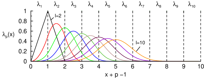
Finally, using eq. 40 and 42 one obtains the expression of the which are polynomial functions of order in (see fig. 2) :
| (43) |
These functions are segments of the uniform sum distribution , i.e. the distribution of the sum of uniform variates on the interval :
| (44) |
From this relation, it is obvious that the functions satisfy the first three conditions mentioned above.
We now consider a fragment of crystal made of construction cells . As these cells are composed of original cells , they partially overlap, and the size of the fragment corresponds to cells . cells in the center contains charges with the nominal values , and cells on each side of the fragment contains partial charges. The latter partial charges are proportional to the coefficients :
| (45) |
These coefficients are represented on fig. 2. The abscise values have been shifted by , so that the origin corresponds to the position of the effective edge of the fragment (i.e. the position of the edge obtained when using original cells without partial charges). One can see that the renormalization of the charges is relatively small. Indeed, even in the case , this renormalization is weaker then for charges at distances larger than .
As already mentioned, the and are polynomial functions of order . It is also interesting to notice that at the junction point between the (resp. ) and (resp. ) functions, the renormalization function and all its the derivatives are continuous, except for the last one ( derivative).
IV Optimized method


We first use the cells to illustrate the convergence of the standard, real-space calculation of the potential established in section II. In order to observe the general behavior of the different methods, we chose the quartz structure, that possesses a reasonable number of atoms per unit cell and not too many symmetries. A cell is constructed for a fixed number of . The cells are used to produce sets of charges of increasing size. The potential and the electric field are calculated at the position of the twelve atoms of the central unit cell .
Fig. 3 a) represents the maximum of the error made on these potential values as a function of the width of the set of charges, fig. 3 b) represents the maximum of the error made on the sixty six differences of potential, and finally fig. 3 c) represents the maximum of the error made on the electric field. As expected the errors decrease as power functions of the width of the set of charges. It fully agrees with eq. 18, 29 and 32. In particular, the fact that the cancellation of a moment of odd order do not increase the convergence rate of the potential at a point, clearly appears. Similarly, the cancellation of even order moment do not improve the convergence rate of the calculation of differences of potential and electric field.


One can see from the previous figures that this standard approach is not the more efficient. Indeed the increase of the number of zero multipolar moments clearly yield a faster convergence rate than the increase of the volume of the system for a fixed value of . Let us therefore fix the width of the volume containing the nominal charge, and let increase. The variation of the maximum error made on the potential, on the potential differences and on the electric field are respectively represented on fig. 4 a), b) and c). One sees that the present approach leads to an exponential convergence of the potential in all cases. The convergence is very fast, since an increase of the set of charges width by two unit cells results in a precision increase by a factor better than . Increasing the number of central cells without partial charges has a small influence on the convergence speed. For the method even becomes less efficient since increasing increases the size of the total set of charges. The best convergence is obtained for . It corresponds to the case where the cell in which the potential is calculated is surrounded by one shell of cells with the nominal charge values.
Finally we compare our method to the famous Ewald’s method which mixes calculation in real space and reciprocal space. This method introduces Gaussian distribution of charge , where the coefficient can be adjusted. Increasing coefficient increases the convergence rate of the real space sum, but slows down the sum in reciprocal space. A width of Gaussian proportional to the characteristic length of the unit cell, which corresponds to , is generally assumed to give a good compromise. We calculated the error made on the value of the potential using the Ewald’s method for different values of around . The results are represented on figure 5, as well as the error of our method obtained for .

Figure 5 reports the error on the potential as a function of the number of construction cells used in the calculation. Let us point out that, while this variable is pertinent for the global convergence rate analysis, for each charge, the Ewald’s method requires an error function evaluation resulting in a non negligible pre-factor, not present in our method and not taken into account in figure 5. One sees that the convergence rate of the present method is comparable with the Ewald’s method. If one is only interested in the potential evaluation at a single point, the Ewald’s method with an optimal parameter is somewhat faster than the present one. One the other hand, once the renormalization have been computed, the value of the potential at any other point of the of the central area can be calculated with a similar precision at little cost. More important, properties using potential integrals or complex potential functions can be more easily evaluated since our method used only algebraic functions.
V Conclusion
Number of authors have searched for a fast converging method for the evaluation of the electrostatic potential in real space. Similarly, many works where done yielding partial results on the convergence rate of such real series. The present work fills the gaps and proposes a general analysis of both the convergence of the potential at one point and of the convergence of differences of potential. Indeed, we gave a general and rigorous proof of the relation (claimed by other authors) between the power law convergence of the series and the number of zero multipolar moments of the crystal construction cell.
Based on these convergence analyses we derived a general real space method with an exponential convergence rate, comparable with the Ewald’s method. The exponential convergence is reached as a function of the number of canceled multipolar moments in the construction cell. The crystal is indeed constructed using overlapping construction cells with renormalized charges. We derived a general analytical expression of the renormalization factors, for any given number of zero multipolar moments.
Finally, we would like to point out that our method warrants continuous and smooth variations of the renormalization factors. This property is of particular interest for molecular dynamic usage since it insures continuous and smooth variations of the ionic forces as a particle crosses the cell boundaries. One can see the present functions as optimized cut-off functions.
References
- [1] P.P. Ewald, Ann. Phys. (Leipzig) 64, 253 (1921).
- [2] H. M. Evjen, Phys. Rev. 39, 675 (1932).
- [3] C. Sousa, J. Casanovas, J. Rubio and F. Illas, J. Comput. Chem 14, 680 (1993).
- [4] S. E. Derenzo, M. K. Klintenberg and M. J. Weber, J. Chem. phys. 112, 2074 (2000).
- [5] V. R. Marathe, S. Lauer and A. X. Trautwein, Phys. Rev. B 27, 5162 (1983).
- [6] J. P. Dahl, J. Phys. Chem. Solids 26, 33 (1965).
- [7] C. K. Coogan, Aust. J. Chem. 20, 2551 (1967).
- [8] A. Gellé, Ph.D. Thesis, Université Paul Sabatier, Toulouse, France, (2004).
- [9] M. A. Epton and B. Dembart, SIAM J. ScI. Comput. 16, 865 (1995).
- [10] J. P. Dahl and M. P. Barnett, Mol. Phys. 9, 175 (1965).
- [11] R. A. Sack, J. Math. Phys. 5, 252 (1964).
- [12] Y.-N. Chiu, J. Math. Phys. 5, 283 (1964).