Properties of Black Hole Radiation from Tunnelling
Abstract
We consider the space-time associated with the evaporation of a black hole by quantum mechanical tunnelling events. It is shown that the surface through which tunnelling occurs is distinct from the global event horizon, and that this has consequences for the radiation reaching future null infinity. A spherical collapse process is modelled, and the radiation expected to be observed at future null infinity is calculated. It is shown that external observers witness an evaporation process that begins as the tunnelling surface is exposed, and ends as the collapsing object passes behind its event horizon. The sensitivity of emitted radiation to the collapse process is illustrated.
1 Introduction
A common interpretation of Hawking radiation [1] is that of virtual particles tunnelling through the horizon. In this picture a virtual pair is nucleated just inside (or just outside) the horizon. A quantum mechanical event then transports the positive energy particle from inside the horizon to the outside (or the negative energy particle from outside to inside). The result is a real particle materialising outside the black hole, and the mass of the hole being reduced. This long considered heuristic explanation of Hawking radiation was recently given a solid basis by Parikh and Wilczek [2]. The calculation they performed took into account the changing geometry of the space-time as the tunnelling events occur, and provides a natural time coordinate with which to parameterise the mass loss of the hole, as well as giving the location of the origin of radiation. Interestingly, it was shown that the spectrum of emitted radiation is not a precise black-body, as had previously been shown in [3], although it was not made clear how this could be linked to the collapse process that formed the hole.
Here we consider a collapse process leading to the formation and subsequent evaporation of a black hole. We model this as a collapsing spherical shell of matter. Once formed, the hole is assumed to decrease in mass by the tunnelling process described above. The resulting geometry (as previously considered by Brown and Lindesay [4, 5, 6]) exhibits a global event horizon that is displaced from the origin of the radiation. The energy-momentum of the escaping radiation is then calculated. It is found, as expected, that an asymptotic observer watching the collapse witnesses an increase in the flux of radiation as he/she is exposed to the surface through which tunnelling occurs. This appears to the external observer as if radiation is being emitted before the collapsing object passes its own event horizon. The flux of radiation then continues to increase until the event horizon is reached. Similar results, by an alternative method, have been found in [7].
It is of interest to determine the sensitivity of the emitted radiation to the collapse process that forms the black hole. As is well known, all information about the collapse is removed in the limit that the event horizon is approached. Only the early radiation is sensitive to it [8]. In the case of a static black hole it is unclear exactly what is meant by ‘early’ (i.e. if this means a short time before the end of evaporation, or in the remote past). In the present case we have both a beginning and an end to the evaporation process: when the tunnelling surface is exposed and when the black hole evaporates completely. This allows an investigation of whether the radiation emitted between these times can contain any information about the structure that collapsed to form the hole. That the tunnelling surface is known to be separate from the global event horizon indicates that this may be the case, as the modes that are infinitely suppressed as the horizon is approached can then be non-zero.
In section 2 we consider the geometry of the system. The mass of the hole is made to decrease as a function of the time coordinate used in the tunnelling calculation [2] (the proper time of a freely falling observer). The resulting line-element is then transformed into double null coordinates, as in [5]. In section 3 we discuss the separation of the global event horizon from the surface . The tunnelling calculation suggests that the outgoing radiation is emitted from , and not the global horizon. This is in good agreement with the results of [16, 17, 18]. Section 4 contains a calculation of the renormalised vacuum expectation value of the energy-momentum tensor in the two dimensional analogue of this space-time, as prescribed by the point splitting method of Davies and Fulling [9]. The corresponding energy-momentum tensor in the Vaidya space-time has been considered in [10, 11]. In section 5 we use the results of the previous calculations to consider the radiation measured by an external observer watching a spherical collapse, and show the extent to which this radiation is effected by the process that formed the hole. A discussion is provided in section 6.
2 Geometry of the system
A natural choice for the parameterisation of tunnelling events through the horizon is the proper time of a radially in-falling observer. This is given by the Panlevé time [12], or river time, , used by Parikh and Wilczek in their calculation of the rate of these events [2]. For a black hole geometry with constant mass, this time coordinate is related to the more usual Schwarzschild time, , by
| (1) |
The Schwarzschild metric can then be written as
| (2) |
When considering events occurring at this coordinate system has a number of advantages over Schwarzschild coordinates. Firstly, surfaces of constant cross the surface , allowing events along to be assigned a time at which they occur. Secondly, as mentioned above, corresponds to the proper time of a freely falling observer along a radial geodesic parameterised by (over-dots denote differentiation with respect to throughout). Furthermore, surfaces of constant are simply Euclidean 3-spaces.
To account for the reduction in mass of the hole due to tunnelling we now parameterise as . (If one were to attempt such a parameterisation in terms of then a curvature singularity would appear at ). This time-dependent Panlevé geometry is the one considered by Brown and Lindesay in [4, 5, 6]. We consider it to be the continuum limit of the near horizon geometry that results from many small, discrete tunnelling events. For simplicity we consider radiated particles to be s-waves, so that by Birkhoff’s theorem their effects on the geometry of the hole can be neglected, other than by reducing the value of . This geometry is similar to the Vaidya metric, but here the mass, , is made a function of the Panlevé time, , used in the tunneling calculation, instead of the advanced time, . This geometry allows the mass loss due to tunneling to be taken into account straightforwardly, as well as allowing the metric to be cast in double null co-ordinates in a simple way.
Consider the retarded and advanced null coordinates [5]
| (3) | ||||
| (4) |
where and must satisfy the integrability conditions
| (5) | ||||
| (6) |
If constant then these equations have the simple solutions and , corresponding to the Schwarzschild solution in null coordinates. If then for a slowly evaporating black hole we can approximate by an expansion about some early moment, , so that . To this order of approximation equations (5) and (6) have the solutions
| (7) | ||||
| (8) |
where are the roots of , and are the roots of . In terms of the new coordinates, defined by (3) and (4), the line-element (2) then takes the form
| (9) |
where and are given by (7) and (8). This geometry will be used to describe the region outside a shell of matter that collapses to form a radiating black hole. Inside, the geometry will be taken to be Minkowski space covered by the retarded and advanced null coordinates, and , such that . The two sets of null coordinates in the two regions can then be related at the boundary between them by the transformations and . If this boundary is at a radial distance , then these functions are given by the differential relations
| (10) | ||||
| (11) |
3 Tunnelling and the horizon
An important feature of the geometry (2) is that the global event horizon (the boundary of the past of future null infinity) is not at . It is displaced by a small amount11 1 Although it has been suggested by some that it may be displaced by a large amount, so that an event horizon may not form at all [7, 15]. [4, 5, 6]. As the global event horizon is a null surface it is described by the outgoing null geodesics
| (12) |
so that only when , the limit where the black hole is not evaporating. For an evaporating hole we have , and so . Under the approximation the location of can then be seen to be given by the positive real solution of
| (13) |
This is exactly the point at which becomes singular, as can be seen from (7). The Penrose diagram for this geometry (see [5] for details) is shown in figure 1, where the global horizon at is represented by a dashed line and the surface is given by a dotted line. The thick solid line represents the trajectory of the shell, .

The question now arises, through which surface are the radiated particles tunnelling: or ? To answer this let us consider the rate of tunnelling , where S is the action along the classically forbidden trajectory. Using Hamilton’s equation, , Parikh and Wilczek [2] find the exponent of this rate to be
| (14) |
Here is the radial momentum of the particle that is tunnelling from to . The particles trajectory is then given by the null geodesics of (2) with replaced by , where is the energy of the particle. They then swap the order of integration and obtain
| (15) |
where the final expression is given provided . It is then noted that if they had instead kept the original order of integration they would have found
| (16) |
If , the value of is then . This shows that the tunnelling events occur through the surface , where the action obtains an imaginary part. This is distinct from the global event horizon at . For further details the reader is referred to the original text [2], and for criticisms and discussion to [13]. This result has also be generalised to other cases [14].
The idea that radiation should be emitted from a surface outside the horizon is not new: It has been considered by Visser [16], di Criscienzo et al [17], and Nielsen [18], as well by Susskind, Thorlacius and Uglum [19] in the form of a ‘stretched horizon’. The stretched horizon was envisaged as a place where information about the micro-physical structure of objects falling into a black hole could be stored, and subsequently encoded in outgoing radiation. In the present study, as in [16, 17, 18], this surface is the place where an outgoing particle trajectory is classically forbidden. Such a surface is a physically meaningful concept at finite times, unlike the surface which requires a knowledge of the global structure of space-time in order to be defined.
4 The energy-momentum of radiation
We will now compute the vacuum expectation value of the energy-momentum tensor of a massless conformal scalar field in the vicinity of the surface , outside of a collapsing shell of matter. This calculation will be in two dimensions and will follow the study of Davies [8], which was performed with constant. The regularisation method employed will be the point splitting method of Davies and Fulling [9]. In this method the product of field operators in the energy-momentum tensor are evaluated as functions of two points along a geodesic. The points are then brought together, and the divergent terms covariantly subtracted. The result is a non-divergent and covariant, renormalised vacuum expectation value for the energy-momentum tensor. Although the two dimensional case has proved a useful tool in understanding semi-classical radiation, one should keep in mind that it may not be exactly analogous to the corresponding case in four dimensions [20]. This method has been previously applied to dynamical black hole space-times in [10, 11].
Following [21] we introduce a new system of null coordinates, and , that cover the space-time both inside and outside the shell of radius . The metric is then given by
| (17) |
where
As this metric is conformally flat, the solutions of the scalar wave equation are the solutions of , which are simply and . The choice ensures these fields can be made to correspond with their usual form in Minkowski space at past null infinity. Furthermore, choosing means that outgoing waves can be matched to incoming waves at , allowing a simple correspondence as they pass through the centre of the shell.
The point splitting procedure of [9] now yields the renormalised energy-momentum tensor for a massless conformal field in the geometry (17) as
| (18) |
where , , and . The components of this tensor can be evaluated using the relations specified above between the three coordinate systems. Inside the shell the non-zero components are, in and coordinates,
| (19) | ||||
| (20) |
whilst outside the shell we have, in and coordinates,
| (21) | ||||
| (22) | ||||
| (23) |
where , , and are given by (7), (8), (10) and (11). The expressions (19)-(23) now give the required form of the energy-momentum tensor for a scalar field in the presence of a collapsing shell of matter, and will be used below to investigate the energy density of radiation measured by observers watching the collapse.
5 Measurements made by asymptotic observers
5.1
Let us briefly review the static limit, , so that , and the results of [8] are retrieved. In this case the third terms in (21) and (22), and the second term in (23), are zero everywhere. The first two terms in each of (21) and (22) are identical, and, along with the first term of (23), represent an energy density in the vicinity of the black hole due to the curvature of Schwarzschild space-time. This energy density vanishes in the limit , and does not contribute to the Hawking radiation measured by asymptotic observers.
The remaining two terms of (21) are functions of the retarded time coordinates only, and can therefore give a non-zero energy density at future null infinity. The last of these terms, , is a function of for finite . As , however, it approaches and so corresponds to the Hawking term. The penultimate term in (21), , matches the mode inside the shell, given by equations (19) and (20), which is initially in-going, then passes through the centre at before becoming an outgoing ray that passes back out through the shell and on to future null infinity. This term is sensitive to the form of , and its pre-factor of , due to the transformation from to , is non-zero for finite . As , however, so that the contribution of this term vanishes in that limit.
When the only relevant non-zero term as is therefore the Hawking one, which is a constant, independent of the process that formed the black hole (i.e. independent of ). For finite this is not the case, and the flux of radiation reaching future null infinity is sensitive to the collapse process. Whether this corresponds to any useful information reaching the asymptotic observer is unclear, as in this case surfaces of finite can be removed to the distant past by the stacking of surfaces of constant against the event horizon. We will now investigate the case in which . As discussed above the source of the radiation in this case is expected to be the surface , which is displaced from the global event horizon at .
5.2
It can be seen that when the first two terms of (21) and (22), and the first term of (23), are still independent of the collapse process. Their forms are modified from the case, as the two functions and are now given by (7) and (8), but they still approach zero as . When we now have three new terms: The third terms in (21) and (22), and the second term in (23). These terms also vanish as , and so do not contribute to any flux at future null infinity22 2 These terms may be badly behaved in the limit due to an unrealistic aspect of the model. This will be commented upon in the discussion section. For further discussion of diverging energy-momentum in dynamical black hole space-times see [10, 22]..
The only non-zero components of the energy-momentum tensor, as , are therefore
These are the same two terms that contribute to the asymptotic flux in the case, but now the and terms, as well as the coordinate transformations between , and , are modified by the non-constant . Substituting (7), (8), (10) and (11) into the expression above, together with the relevant transformations from and to , allows these two terms to be evaluated as functions of . Due to the complicated form of the resulting expressions we choose not to show them explicitly here, but rather to present them as plots. This will demonstrate how the present case differs from the case, which we will display in parallel for comparison.
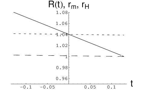
For illustrative purposes let us consider and , so that at . The trajectories of , and are then shown in figure 2 as the solid line, the dotted line and the dashed line, respectively. Before the shell is outside of both and . Between and the shell is between and , and after the shell is inside the global horizon. We will refer to this choice of parameters as “hole 1”.
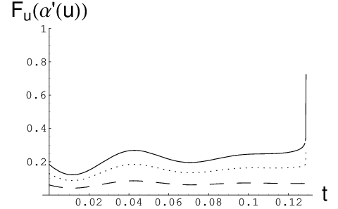
for hole 1 can be readily calculated and is shown in figure 3(a) as a function of along the trajectory . Similarly, is shown in figure 3(b). These plots have been normalised so that when , the moment the shell crosses the global event horizon. For comparison we also show in figures 3(a) and 3(b) the results that would have been obtained for a black hole evaporating at half the rate (“hole 2”, the dotted lines) and a black hole with constant mass (“hole 3”, the dashed lines). In both of these cases the trajectory of the in-falling shell is kept the same as for hole 1, and both have been chosen so that the of all three holes are equal at the moment .
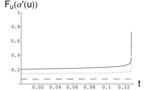
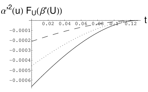
It can be seen from figure 3 that the value of for hole 3 is approximately constant over the time scale being considered, at the Hawking rate of . For holes 1 and 2 can be seen to be a slowly increasing function of , that becomes rapidly increasing as . The value of can be seen to approach zero for all three holes as , as expected. This is due to in this limit.
Let us now consider what the observer at infinity measures. To find this we must transform the plots above from to , the proper time of an asymptotic observer, by
| (24) |
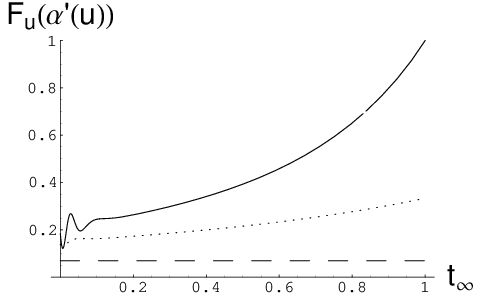
This expression relates the two time coordinates via the retarded time . The two terms and are now given as function of in figures 4(a) and 4(b). These plots are normalised by the value of for hole 1 at , and the new time coordinate for holes 1 and 2 have been chosen so that when the asymptotic observer sees . (This is not possible in the static case as the surface is degenerate with ). Units have been chosen so that when the asymptotic observer sees , in each case.
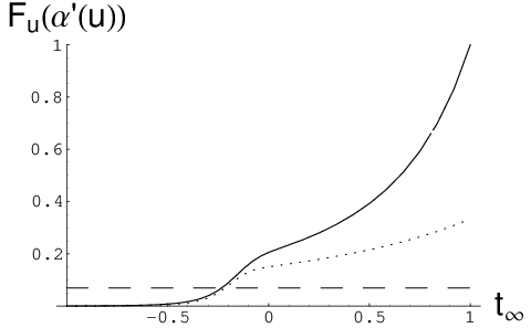
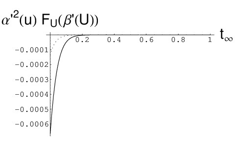
These plots are the same as those of figure 3, but they have been stretched near and squashed near , giving them a considerably different appearance. The stretching involved increases as the rate of evaporation decreases, diverging in the limit of a static hole. Hence the lines corresponding to hole 3 are now straight, and equal to zero in the case of figure 4(b).
The observer at infinity watching holes 1 and 2 sees an energy density in the mode that rises as the shell is seen to pass , and subsequently increases at a steady rate. This is due to the surfaces of constant stacking up against the global horizon, and stretching out the spikes seen in figure 3(a). That the radiation increases as the shell crosses is in support of the conjecture that the radiation is originating from this surface, as found directly in the tunnelling calculation.
Figure 4(b) shows that for holes 1 and 2 the contribution from , as witnessed by the asymptotic observer, becomes exponentially small soon after the shell crosses . Again, this is due to the stacking of surfaces of constant against the global horizon, and the resulting stretching of figure 3(b). In the vicinity of , however, while this component is small, it is still non-zero. This is of interest as is known to be sensitive to the collapse process that formed the hole [8].
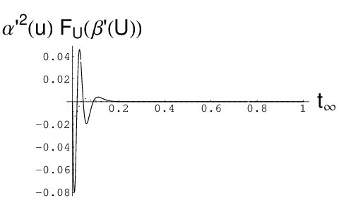
To consider the degree to which the outgoing radiation is sensitive to the collapse process, let us now perturb the in-falling trajectory of the shell by a small amount, so that . This is a small enough perturbation that the plot of the trajectory of the in-falling shell is indistinguishable from figure 2. However, the effects on and are not negligible, and are shown in figure 5. The same scalings and origin have been chosen as above. Perturbations to the infall trajectory could result from imperfections in spherical symmetry, internal stresses, or interactions of the shell with other objects. Here we simply wish to illustrate the sensitivity of the emitted raditiation to the collapse process, and so add an ad hoc oscillation to the shell’s trajectory. It can be seen such oscillations, although small, have a discernible effect on the outgoing radiation of the holes. Both functions and can be seen to oscillate around their unperturbed values, as shown in figure 3. These oscillations are particularly apparent in .
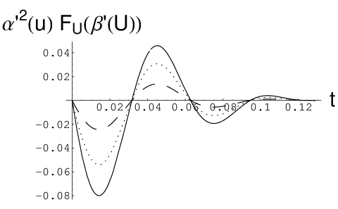
Now let us consider the radiation measured by an asymptotic observer watching the perturbed shell collapse. Any features present in the plots in figure 5 should also be present in the radiation he/she measures, although it will be effected by the stretching and squashing involved in the transformation from to . Using (24) we find that and are given as functions of as shown in figure 6. For holes 1 and 2, the oscillations that were present in figure 5 are again apparent, but now restricted to be observable only in the vicinity of (due to the stacking of surfaces of constant against the global horizon). The infinite stretching in the case of hole 3 is enough to remove the oscillations that were present in figure 5 to the infinite past.
6 Discussion
We have considered the case of a black hole that forms from the collapse of a spherical shell, and decays via tunnelling events. In this case the mass parameter of the hole is made a function of the Panlevé time, , and the surface separates from the global event horizon by a small amount. The tunnelling events occur at , and not at the global event horizon. This displacement has consequences for the emission of Hawking radiation, and for its observation by asymptotic observers watching the collapse.
The energy-momentum tensor of a massless conformal scalar field is obtained in the two dimensional analogue of this space-time, and the flux of radiation measured by an asymptotic observer is calculated. The asymptotic observer witnesses radiation that initially increases at about the time he/she sees the collapsing shell cross , and increases at a steady rate thereafter. This supports the idea that the Hawking radiation is emitted from the vicinity of the surface [16, 17, 18], and that after this surface is exposed to asymptotic observers he/she witnesses radiation from a hole that is slowly increasing in temperature.
Radiation originating from outside of the global event horizon contains modes that are sensitive to the collapse process [8]. This sensitivity is illustrated by perturbing the collapsing shell with a small oscillation. The effects of this on the modes that escape to future null infinity are clearly visible, and only vanish in the limit that the global horizon is approached. For the static model the infinite stacking of surfaces of constant retarded time against the global horizon removes these modes to the remote past, so that it is unclear whether they have any observational significance. This is not the case in the non-static models. Here the sensitivity of the emitted radiation to the collapse process is clearly visible, but restricted to be observable only at the beginning of the evaporation process. Nevertheless, an observer who measures all of the radiation emitted from the hole may, in principle, be able to extract some information about the collapse process that formed it.
There are a number of ways in which this study could be improved. In
particular, one could parameterise as a function of
in a more satisfactory way. Here we assumed a function of the form ,
in order to get explicit, exact solutions. While this is likely to be valid
for the early stages of evaporation (being the first term of a
series expansion), it is unlikely to be a good approximation
during the late stages. Ideally one would like to find solutions with
more general . A further problem is the behaviour
of the model as , when the black hole evaporates
completely [10, 22]. In this limit (depending on the form of ) the
scalar curvature invariants associated with the space-time (2) may diverge, indicating a
singularity33
3
This is the origin of the bad behaviour mentioned
in the footnote of section 5.2.. This shows that a
continuum limit for is not appropriate at the end point of
evaporation, and that a cutoff should be introduced beyond which a
more appropriate method is used.
Acknowledgements
I am grateful to Pedro Ferreira and Philip Candelas for helpful discussions, and to Jesus College for support.
References
- [1] S. W. Hawking, Comm. Math. Phys. 43, 199 (1975).
- [2] M. K. Parikh and F. Wilczek, Phys. Rev. Lett. 85, 5042 (2000).
- [3] P. Kraus and F. Wilczek, Nucl. Phys. B 433, 403 (1995). E. Keski-Vakkuri and P. Kraus, Nucl. Phys. B 491, 249 (1997).
- [4] J. Lindesay, Foundations of Physics 37, 1181 (2007).
- [5] B. A. Brown and J. Lindesay, arXiv:0710.2032 (2007).
- [6] B. A. Brown and J. Lindesay, arXiv:0802.1660 (2008).
- [7] T. Vachaspati, D. Stojkovic and L. M. Krauss, Phys. Rev. D 76, 024005 (2007). T. Vachaspati and D. Stojkovic, Phys. Lett. B 663, 107 (2008).
- [8] P. C. W. Davies, Proc. R. Soc. Lond. 351, 129 (1976).
- [9] P. C. W. Davies and S. A. Fulling, Proc. R. Soc. Lond. 348, 393 (1975).
- [10] W. A. Hiscock, Phys. Rev. D 23, 2813 (1981).
- [11] R. Balbinot, Phys. Rev. D 33, 1611 (1986).
- [12] P. Panlevé, C. R. Acad. Sci. (Paris) 173, 677 (1921).
- [13] B. D. Chowdhury, Pramana 70, 593 (2008). E. T. Akhmedov, V. Akhmedova and D. Singleton, Phys. Lett. B 642, 124 (2006). E. T. Akhmedov, V. Akhmedova, T. Pilling and D. Singleton, Int. J. Mod. Phys. A 22, 1705 (2007). V. Akhmedova, T. Pilling and A. de Gill and D. Singleton, arXiv:0804.2289, (2008). T. K. Nakamura, arXiv:0706.2916 (2007). P. Mitra, Phys. Lett. B 648, 240 (2007).
- [14] K. Srinivasan and T. Padmanabhan, Phys. Rev. D 60, 24007 (1999). S. Hemming and E. Keski-Vakkuri, Phys. Rev. D 64, 044006 (2001). S. Shankaranarayanan, T. Padmanabhan and K. Srinivasan, Class. Quant. Grav. 19, 2671 (2002). A. J. M. Medved, Phys. Rev. D 66, 124009 (2002). E. C. Vagenes, Phys. Lett. B 559, 65 (2003). T. Padmanabhan, Mod. Phys. Lett. A 19, 2637 (2004). A. J. M. Medved and E. C. Vagenas, Mod. Phys. Lett. A 20, 2449 (2005). M. Arzano, A. J. M. Medved and E. C. Vargenas, JHEP 0509, 037 (2005). Q. Q. Jiang, H. L. Li, S. Z. Yang and D. Y. Chen, Mod. Phys. Lett. A 22, 891 (2007).
- [15] S. A. Haywood, Phys. Rev. Lett. 96, 031103 (2006). A. B. Nielsen, arXiv:0711.0313 (2007). A. B. Nielsen, arXiv:0804.4435 (2008).
- [16] M. Visser, Int. J. Mod. Phys. D 12, 649 (2003).
- [17] R. Di Criscienzo, M. Nadalini, L. Vanzo, S. Zerbini and G. Zoccatelli, arXiv:0707.4425 (2007).
- [18] A. B. Nielsen, arXiv:0802.3442 (2008).
- [19] L. Susskind, L. Thorlacius and J. Uglum, Phys. Rev. D 48, 3743 (1993).
- [20] V. Frolov, P. Sutton and A. Zelnikov, Phys. Rev. D 61, 024021 (1999).
- [21] P. C. W. Davies, S. A. Fulling and W. G. Unruh, Phys. Rev. D 13, 2720 (1976).
- [22] T. P. Singh and C. Vaz, Phys. Lett. B 481, 74 (2000).