Effective temperature for hopping transport in a Gaussian DOS
Abstract
For hopping transport in disordered materials, the mobility of charge carriers is strongly dependent on temperature and the electric field. Our numerical study shows that both the energy distribution and the mobility of charge carriers in systems with a Gaussian density of states, such as organic disordered semiconductors, can be described by a single parameter – effective temperature, dependent on the magnitude of the electric field. Furthermore, this effective temperature does not depend on the concentration of charge carriers, while the mobility does depend on the charge carrier concentration. The concept of the effective temperature is shown to be valid for systems with and without space-energy correlations in the distribution of localized states.
pacs
72.20.Ht, 72.20.Ee, 72.80.Le, 72.80.NgI Introduction
For many years much attention of researchers has been devoted to the effect of high electric fields on the hopping mobility of charge carriers in organic disordered materials, such as conjugated and molecularly doped polymers and semiconducting organic glasses.[1, 4, 2, 3] Two peculiarities in the dependence of the carrier mobility on the electric field are usually discussed in the literature. One of them is the apparent decrease of the mobility with rising field at relatively low fields and high temperatures reported in several time-of-flight studies.[5, 6, 7, 1] The other one is the very strong non-linear increase of the carrier mobility with electric field at low temperatures and high fields.[1, 4, 2, 3] While the former peculiarity has been attributed [8, 3] to misinterpretation of experimental data, the latter one has been confirmed in numerous experimental studies and it is currently in the focus of intensive theoretical research. Before we turn to discussing this research, it is worth noting that very similar non-linear effects with respect to the applied electric field have been known since decades for transport phenomena in the inorganic noncrystalline materials, such as amorphous semiconductors. Indeed, strong nonlinearities in amorphous semiconductors were observed for the field dependence of the dark conductivity,[9, 10] of the photoconductivity,[11] and of the charge carrier drift mobility [9, 12, 13] at high electric fields. While the field-dependent hopping conductivity at low temperatures was always a challenge for a theoretical description, the theories for temperature dependence of the hopping conductivity at low electric fields were successfully developed for all transport regimes listed above (see for instance Ref. 3 and references therein). Furthermore, it has been shown that the effect of a strong electric field on transport coefficients in amorphous semiconductors can be effectively described by replacing the temperature parameter in the formulas for the low-field temperature-dependent mobility and conductivity by an effective temperature , dependent on the magnitude of the electric field . Shklovskii [14] was the first who recognized that, for hopping conduction, a strong electric field plays a role similar to that of temperature. In the presence of the field, the number of sites available for charge transport is essentially enhanced in the direction prescribed by the field. The distance between sites available for hopping transport shortens and hence electrons can move faster.[14] The concept of the effective temperature has been studied in detail for systems with an exponential energy distribution of localized states usually assumed for inorganic noncrystalline materials:
| (1) |
where is the concentration of localized states and is the energy scale of the distribution. By studying the steady-state energy distribution of electrons in numerical calculations and computer simulations [15, 16] and by computer simulations of the steady-state hopping conductivity and the transient energy relaxation of carriers [17] the following result has been found. The whole set of transport coefficients can be represented as a function of a single parameter :
| (2) |
with and values of in the range - depending on which transport coefficient is considered.[17] In this expression is the localization length of charge carriers in the localized states, is the elementary charge, and is the Boltzmann constant. Herewith the problem of nonlinearities of transport coefficients with respect to the applied electric field for inorganic noncrystalline materials with the density of states (DOS) described by Eq. (1) has been solved.
Let us now turn to the organic disordered materials. In such systems the density of states involved in the hopping transport of charge carriers is believed to be not purely exponential as in Eq. (1), but rather to be described by a Gaussian energy distribution: [1, 18, 19, 4, 2, 3]
| (3) |
Numerous computer simulations have been devoted to studying the field nonlinearities of transport coefficients in the hopping regime in such systems. Two models of disordered organic materials were considered: the so-called Gaussian disorder model (GDM) suggested by Bässler et al.[1] and the so-called correlated disorder model (CDM) considered by Garstein and Conwell, [20] by Dunlap et al.,[21] and by Novikov et al.[22, 23] In both models, the field dependence of carrier mobility has been studied by computer simulations. While analytical calculations have been carried out in order to justify the CDM, [21, 22, 23] a consistent analytical theory for the field dependence of the hopping mobility in a Gaussian DOS is still missing.
It is tempting to try to apply the concept of the effective temperature to organic disordered systems with the Gaussian DOS described by Eq. (3), since this concept has proven to be very successful for inorganic systems with the exponential DOS described by Eq. (1). The idea that a strong electric field leads to heating of the charge carriers in organic materials has already been considered in several theoretical studies. Recently Preezant and Tessler [24] performed such a study in the framework of an analytical approach that artificially decouples the energy-dependent factors in the hopping transport from the space-dependent factors. However, this approach has been shown [3, 25] to be unsuitable for describing hopping transport processes in disordered materials. Moreover, such an approach leads to an effective temperature that essentially differs from the one considered in previous studies for inorganic materials [14, 15, 16, 17, 3] where the effective temperature arises from the interplay between spatial- and energy dependent factors in hopping processes. Li, Meller and Kosina[26] recently approached this problem by inserting the dependence of transition rates on the electric field and that of the percolation threshold into the percolation theory of Vissenberg and Matters [27]. More recently, Limketkai et al.[28] exploited the concept of the effective temperature in order to account for the strong field nonlinearity of the conductivity and carrier mobility observed in organic semiconductors.[29] Limketkai et al. chose the expression for the effective temperature in the form of Eq. (2) with and . It has been proven however[17] that such expression for the effective temperature with cannot be considered as suitable. Indeed, suppose the conductivity is dependent on solely. Then
| (4) |
In the Ohmic transport regime at , the conductivity must be field independent, implying that
| (5) |
The function described by Eq. (2) with obviously does not fulfill this condition. However, any function of this kind with is consistent with Eq. (5) along with the necessary condition at and at .
Therefore the challenging problem arises to find out whether the concept of the effective temperature is applicable to systems with a Gaussian DOS and if yes, what is the expression for . We try to answer these questions in the present study. For this purpose we follow the idea of Marianer and Shklovskii [15] to look at the energy distribution of charge carriers using the numerical method of nonlinear balance equations suggested by Yu et al.[31, 30, 32, 33] and apply it to electron transitions in a Gaussian DOS. Preliminary data for the energy distribution of charge carriers in the GDM at low carrier concentrations confirmed the concept of the effective temperature.[34]
The paper is organized as follows. In Sec. II the numerical method used in our study is described. In Sec. III the results for the energy distribution function of charge carriers in the GDM are presented. It is shown that at finite temperatures and electric fields the energy distribution of charge carriers in a Gaussian DOS can be well described by the Fermi-Dirac distribution function characterized by given by Eq. (2) with and thus confirming the applicability of the concept of the effective temperature to organic disordered solids. Furthermore, we show that the expression for is stable against changes in the concentration of charge carriers. Numerical results obtained for the mobility of charge carriers also confirm the concept of the effective temperature for the GDM. In Sec. IV the corresponding results for the CDM are presented. They prove that the concept of the effective temperature is valid also for correlated systems. Concluding remarks are gathered in Sec. V.
II Numerical method
In order to check the validity of the concept of the effective temperature, we solved a system of non-linear balance equations with respect to the steady-state occupation probabilities of sites and checked, following the idea of Marianer and Shklovskii, [15] whether this distribution can be fitted by a Fermi–Dirac distribution
| (6) |
with some single parameter . We also calculated the carrier drift velocity along the field direction and the corresponding mobility at different temperatures and electric fields and checked whether the mobility can be described as a function of a single parameter combined from the temperature and the field strength .
The balance equation for the occupation probability of a site has the form [31, 30, 32, 33]
| (7) |
where the rate of jumping from site to site is given by the Miller–Abrahams formula,
| (8) |
Here is the difference between energies of states and , is the distance between these states, and is the attempt-to-escape frequency. While in the initial work of Marianer and Shklovskii [15] the limit of a low concentration of charge carriers was considered and the balance equations were linearized, we study a system with finite number of charge carriers . In order to solve the system of the nonlinear balance equations we use the iterative numerical procedure suggested by Yu et al. [31, 30, 32, 33] The balance equation (7) is rewritten in the form
| (9) |
where the right hand side does not contain . This expression is used iteratively to find a solution to Eq. (7). In each iteration step, all are updated. If has already been calculated in the current step, this value is used, otherwise the result from the previous step is used. This so called implicit iteration is necessary for obtaining convergence. [30] In the sums over , only the most important transitions are needed. We have considered jumps shorter than a cut-off length , chosen so large that it does not affect the transport parameters.
The procedure is repeated until the relative change of any one of the probabilities is smaller than . We note that the solution seems to converge faster if the sites are placed on a lattice than at random. When the localization length is small, more iterations are needed, but the cut-off length can be reduced.
If an electric field is applied in direction, the difference in energy between sites and is given by
| (10) |
When the probability distribution of the charge carriers over the sites is known, the drift velocity of the carriers along the field and their mobility are given by
| (11) |
We studied a system of sites distributed randomly within a cube with a side length . Each site has a random energy , from a Gaussian distribution with the width . The density of states is given by Eq. (3). Periodic boundary conditions were applied in all directions. The calculations were performed in dimensionless units, where the width of the DOS , the site concentration , the Boltzmann constant , elementary charge , and attempt-to-jump frequency are equal to unity.
We used a system containing sites inside a cube with side length . The localization length was varied between and , while the particle concentration was varied in the interval between and .
For each choice of , , concentration , and localization length , a number of realizations of the system were generated and the steady state occupation probabilities were determined. For each realization, the carrier mobility and effective temperature were calculated. The magnitudes of the effective temperaures obtained with different realizations of the system were equal to each other within the accuracy of one percent.
The effective temperature was determined from the occupation probabilities with a linear fit of as a function of ,
| (12) |
This approach works well when the variation in occupation probabilities for sites with similar energies is small. When the variation is larger, we found it better to produce a histogram of and then fit to this histogram as above. The histogram approach seems more correct, since it uses the average occupation probability at a given energy, in contrast to the direct fit that uses the average of . All results for effective temperature presented below were obtained with the histogram method. The parameters and in Eq. (2) were determined by simultaneous fitting of all data points to the surface given by this equation.
In the next Section we present the results of calculations for a system without any correlation between site energies and their spatial positions (GDM). In Section IV we present the results of calculations for the CDM – a system, in which the energies of neighboring sites are correlated. In order to introduce correlations, we generate an initial energy for each site with a Gaussian distribution. We then calculate the real energy for each site by averaging the initial energies of all sites inside the correlation radius , in accord with the recepie suggested by Garstein and Conwell. [20] This averaging procedure has two effects. It will introduce a correlation in energy between spatially close sites and it will decrease the width of the energy distribution. In order to keep the width of the energy distribution independent of the correlation length, the site-energies were rescaled to provide the initial energy width . We discuss these effects of space–energy correlations in more detail in Section IV.
At very high electric fields, when the energy landscape is strongly sloped along the field direction and the energy differences between the successive states become negative as given by Eq. (10), the carrier drift velocity saturates and becomes field-independent.[1] We study the range of electric fields, which are less than the field at which the velocity saturates.
III Effective temperature for systems without space-energy correlations


In Fig. 1 the numerical results are shown for the occupation probability for each site, as a function of site energy, for three different charge concentrations. The inset shows the same data on a logarithmic scale.
At low concentrations, the data can be fitted by a Boltzmann distribution with a parameter , while the data at high concentrations show a Fermi-Dirac shape, remarkably corresponding to the same parameter . Furthermore, Fig. 2 shows that the value of does not depend on the carrier concentration . These results are really remarkable because they mean that the concept of the effective temperature is valid for systems with a Gaussian density of states (so far it has been proven only for exponential DOS described by Eq. (1)) and that the parameter is universal with respect to the concentration of charge carriers in the system under study.
In Fig. 3 we bring together all the calculation results obtained for various field strengths in the range and for various temperatures in the range for concentration of carriers and , in the form of a three-dimensional plot of , obtained by the best fit of the calculated energy distributions by a Fermi-Dirac function. Also the surface determined by Eq. (2) with parameters is shown in this figure. One can see an excellent agreement between the calculated results and Eq. (2) with these parameters.


As described in the previous Section, we also studied the mobility of charge carriers with respect to the applicability of the concept of the effective temperature. In Fig. 4 the dependences of the carrier mobility as a function of determined from the fits of the energy distribution function are shown for different concentrations of charge carriers. These data were obtained for various field strengths in the range and for various temperatures in the range . The data were averaged over three realizations. For the chosen parameters, it appears not important whether the mobilities or the inverse mobilities were averaged. While the magnitude of the mobility appears sensitive to the concentration of carriers, in agreement with the results obtained previously by several research groups, [31, 30, 33, 32, 35, 25, 27, 36, 37, 38, 39] the magnitude of the effective temperature for the given pair () does not indicate any dependence on .
Therefore one can conclude that for the GDM, i.e., for a disordered system with a Gaussian distribution of energies and without any correlations between spatial positions of hopping sites and their energies, the concept of the effective temperature is valid. In the next Section we present results for the CDM, i.e. for the correlated system.
IV Effective temperature for systems with space-energy correlations
In this Section we study the effect of the space-energy correlations on the interplay between the temperature and the electric field with respect to the validity of the concept of the effective temperature.

In Fig. 5 the numerical results are shown for the occupation probability for each site as a function of site energy for three different charge concentrations at correlation length . The inset shows the same data on a logarithmic scale. In analogy to the uncorrelated system, at low concentrations the data can be fitted by a Boltzmann distribution with a parameter , while the data at high concentrations show a Fermi-Dirac shape corresponding to the same parameter as for low concentration.
Fig. 6 shows the effective temperature as a function of the correlation length . The effective temperature strongly depends on the correlation length, thus Eq. (2) is not directly applicable to a system with space-energy correlations.
Before discussing the carrier mobility in a correlated system one should note the following. When the space-energy correlations are introduced as described in Sec. II, the effective width of the energy distribution of localized states decreases. Furthermore this width becomes smaller with increasing . Therefore one can expect that with increasing the mobility would increase just because of diminishing the energetic disorder due to the effect of correlations. In order to compare the carrier mobilities in systems with different correlations and the same energy disorder, one should therefore rescale the width of the energy distribution in the correlated systems and bring it to the value initially ascribed to the uncorrelated system.[20] The effect of correlations on the carrier mobility has already been studied by computer simulations, though in the frame of the lattice model and not with respect to the validity of the effective temperature.[20] In order to compare our results with those of previous studies we also have simulated mobilities in correlated systems within a lattice model along with simulations in the random model.
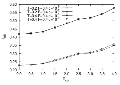
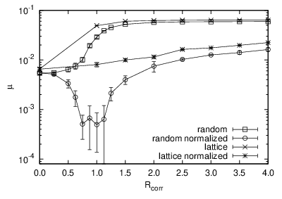

Fig. 7 shows the mobility as a function of the correlation length with randomly placed sites and with sites on a lattice for both cases: with and without rescaling (normalization) of the width of the energy distribution. As expected, without rescaling the mobility always increases with the increase of the correlation length . However in the rescaled system there is an apparent difference between the lattice model and the random model with respect to the dependence of the mobility on the correlation length. While in the lattice model the mobility monotonously increases with in accord with the results of prevous studies,[20] in the random model the dependence of on appears non-monotonous. At mobility decreases with . The reason for the low mobility at could be the following. The normalization (rescaling) procedure creates a small number of sites with very low energies. While the general shape of the DOS for the correlated system is Gaussian, and the variance of the DOS is normalized to be equal to the variance of the uncorrelated system, the DOS of the correlated system has longer tails, and the low-energy tail greatly reduces the carrier mobility. The sites in the tail are those sites that initially had a low energy, and have no neighbors within the distance . Thus they are unaffected by the averaging but are still rescaled with the normalization factor, which is typically close to 2 for . This idea is supported by data shown in Fig. 8. The dip in the mobility disappears when the charge carrier concentration is increased, and the deep states are filled.
V Conclusions
The concept of the effective temperature has been shown to be valid for a system with Gaussian DOS with and without space-energy correlations in the distribution of localized states. From the numerical results for uncorrelated systems one can conclude that the effective temperature is described by Eq. (2) with parameters . Remarkably the validity of the concept of the effective temperature with very close numerical parameters has recently been reported on the basis of experimental study on the inorganic disordered material a-Si:H.[40] This quantitative agreement between experimental data and the results of our calculations could mean that in the material studied in [40] the distribution of localized states can be described by the Gaussian disorder model with uncorrelated distribution of localized states. Note that the effective temperature in our numerical calculations has been proven to be independent of the charge carrier concentration.
Acknowledgements.
F. J. wants to thank Prof. P. Bobbert for valuable discussion regarding the iterative solution method. The calculations were performed at CSC, the Finnish IT center for science. Financial support from the Academy of Finland project 107684 and the TEKES NAMU project, from the Deutsche Forschungsgemeinschaft and that of the Fonds der Chemischen Industrie is gratefully acknowledged.References
- [1] H. Bässler, Phys. Stat. Sol. (b) 175, 15 (1993).
- [2] G. Hadziioannou and P. F. van Hutten, eds., Semiconducting Polymers (John Wiley & Sons, Inc., New York, 2000).
- [3] S. Baranovski, ed., Charge Transport in Disordered Solids with Applications in Electronics (John Wiley & Sons, Ltd, Chichester, 2006).
- [4] M. Pope and C. E. Swenberg, Electronic Processes in Organic Crystals and Polymers (Oxford University Press, Oxford, 1999).
- [5] A. Peled and L. B. Schein, Chem. Phys. Lett. 153, 422 (1988).
- [6] L. B. Schein, Phil. Mag. B. 65, 795 (1992).
- [7] M. Abkowitz, Phil. Mag. B 65, 817 (1992).
- [8] A. Hirao, H. Nishizawa, and M. Sugiuchi, Phys. Rev. Lett. 75, 1787 (1995).
- [9] C. E. Nebel, R. A. Street, N. M. Johnson, and C. C. Tsai, Phys. Rev. B 46, 6803 (1992).
- [10] A. Nagy, M. Hundhausen, L. Ley, G. Brunst, and E. Holzenkämpfer, J. Non-Cryst. Solids 164-166, 529 (1993).
- [11] R. Stachowitz, W. Fuhs, and K. Jahn, Phil Mag B 62, 5 (1990).
- [12] H. Antoniadis and E. A. Schiff, Phys. Rev. B 43, 13957 (1991).
- [13] K. Murayama, H. Oheda, S. Yamasaki, and A. Matsuda, Solid State Commun. 81, 887 (1992).
- [14] B. I. Shklovskii, Sov. Phys. Semicond. 6, 1964 (1973).
- [15] S. Marianer and B. I. Shklovskii, Phys. Rev. B 46, 13100 (1992).
- [16] S. D. Baranovskii, B. Cleve, R. Hess, and P. Thomas, J. Non-Cryst. Sol 164-166, 437 (1993).
- [17] B. Cleve, B. Hartenstein, S. D. Baranovskii, M. Scheidler, P. Thomas, and H. Bässler, Phys. Rev. B 51, 16705 (1995).
- [18] B. Hartenstein and H. Bässler, J. Non-Cryst. Solids 190, 112 (1995).
- [19] R. Schmechel, Phys. Rev. B 66, 235206 (2002).
- [20] Y. N. Garstein and E. M. Conwell, Chem. Phys. Lett. 245, 351 (1995).
- [21] D. H. Dunlap, P. E. Parris, and V. M. Kenkre, Phys. Rev. Lett. 77, 542 (1996).
- [22] S. V. Novikov, D. H. Dunlap, V. M. Kenkre, P. E. Parris, and A. V. Vannikov, Phys. Rev. Lett. 81, 4472 (1998a).
- [23] S. V. Novikov, D. H. Dunlap, and V. M. Kenkre, Proc. SPIE 3471, 181 (1998b).
- [24] Y. Preezant and N. Tessler, Phys. Rev. B 74, 235202 (2006).
- [25] R. Coehoorn, W. F. Pasveer, P. A. Bobbert, and M. A. J. Michels, Phys. Rev. B 72, 155206 (2005).
- [26] L. Li, G. Meller, and H. Kosina, Microelectronics Journ. 38, 47 (2007).
- [27] M. C. J. M. Vissenberg and M. Matters, Phys. Rev. B 57, 12964 (1998).
- [28] B. N. Limketkai, P. Jadhav, and M. A. Baldo, Phys. Rev. B 75, 113203 (2007).
- [29] W. Brütting, S. Berleb, and A. G. Mückl, Org. Electron. 2, 1 (2001).
- [30] Z. G. Yu, D. L. Smith, A. Saxena, R. L. Martin, and A. R. Bishop, Phys. Rev. B 63, 085202 (2001).
- [31] Z. G. Yu, D. L. Smith, A. Saxena, R. L. Martin, and A. R. Bishop, Phys. Rev. Lett. 84, 721 (2000).
- [32] W. F. Pasveer, J. Cottaar, P. A. Bobbert, and M. A. J. Michels, Synth. Met. 152, 157 (2005a).
- [33] J. Cottaar and P. A. Bobbert, Phys. Rev. B 74, 115204 (2006).
- [34] F. Jansson, S. D. Baranovskii, G. Sliaužys, R. Österbacka, and P. Thomas, Phys. Stat. Sol (c) 5, 722 (2008).
- [35] W. F. Pasveer, J. Cottaar, C. Tanase, R. Coehoorn, P. A. Bobbert, P. W. M. Blom, D. M. de Leeuw, and M. A. J. Michels, Physical Review Letters 94, 206601 (2005b).
- [36] H. C. F. Martens, I. N. Hulea, I. Romijn, H. B. Brom, W. F. Pasveer, and M. A. J. Michels, Phys. Rev. B 67, 121203(R) (2003).
- [37] Y. Roichman, Y. Preezant, and N. Tessler, Phys. Stat. Sol. (a) 201, 1246 (2004).
- [38] S. D. Baranovskii, I. P. Zvyagin, H. Cordes, S. Yamasaki, and P. Thomas, Phys. Stat. Sol. (b) 230, 281 (2002a).
- [39] S. D. Baranovskii, I. P. Zvyagin, H. Cordes, S. Yamasaki, and P. Thomas, J. Non-Cryst. Solids 299, 416 (2002b).
- [40] T. Aoki, N. Ohrui, C. Fujihashi, and K. Shimakawa, Phil. Mag. Lett. 88, 9 (2008).