The quest for the fundamental building blocks and laws of the world surrounding us has been a driving force to mankind since its early days. The idea that nature consists of small, invisible constituents was first expressed by the ancient Greek Democritus in the fifth century BC. It was not until the nineteenth century AD that this idea was picked up again and embedded in a scientific context. Over time experiments discovered ever smaller substructures, from atoms to electrons and hadrons, and thereon to quarks. From a theoretical point of view, the aim is to embed these experimental results in a model which is based on as few assumptions as possible and can explain all other physical effects.

The currently established model which performs this task is the Standard Model of elementary particle physics [1, 4]. It is one of the best-tested theories of contemporary physics. All known elementary particles are accommodated in this model. Solely the scalar Higgs boson [5] is included in the theory, but could not be found in experiments so far [10]. It is this particle which is assumed to be responsible for the masses of the fermions and weak gauge bosons.

In spite of its success, the Standard Model also has its insufficiencies, and new theories are searched for, which might provide an even better description of nature. One of the most popular ones is supersymmetry [11]. It extends the two, fundamental symmetries of the Standard Model, the Poincaré group and the non-Abelian gauge group $SU(3)_{C}\otimes SU(2)_{L}\otimes U(1)_{Y}$ of strong, weak and electromagnetic interactions, by an anticommuting operator which induces an equal number of bosonic and fermionic states.

The search for supersymmetry and the Higgs boson are main tasks of the Large Hadron Collider (LHC) at CERN. It will start operation in mid-2007 and provide a wealth of data. To verify or falsify theories and to relate this data to parameters of a model, it is necessary to calculate precise theoretical predictions, which match the accuracy which LHC will be able to obtain. As both the Standard Model and its supersymmetric extension are defined as perturbative theories with a series expansion in Planck’s constant $\hbar$ , the inclusion of effects beyond leading order is often necessary.

In this thesis production processes for Higgs bosons in the Standard Model and its supersymmetric extension, the Minimal Supersymmetric Standard Model (MSSM) [12], at hadron colliders are considered. The calculations are performed at the one-loop level and include the SUSY-QCD corrections, i.e. corrections with squarks and gluinos running in the loop, for the MSSM Higgs bosons.

The outline of this thesis is as following. First, a short introduction to the Standard Model (SM) is given in chapter 2. Special emphasis is put on the Higgs sector of the SM. Here also a possible extension including higher-order operators is discussed. Despite being a well-tested theory, the Standard Model also has its shortcomings, which are mentioned in the last section of this chapter.

Out of the possible extensions of the Standard Model which aim to solve these deficencies, supersymmetry is the most popular one, as it is appealing from both an experimental and a theoretical point of view. Its discussion in chapter 3 of this dissertation starts with the basic principles of the theory. After the necessary ingredients to build a phenomenologically viable model are investigated, the focus is put on the simplest supersymmetric extension of the Standard Model, the Minimal Supersymmetric Standard Model (MSSM) [12]. The Lagrangian of the MSSM after supersymmetry breaking is written down and the particle content of the model is explained.

Chapter 4 is concerned with the methods of regularization and renormalization. The first one is necessary to cancel the divergences which appear in the calculation of one-loop cross sections, and renders the amplitudes finite. Renormalization then restores the physical meaning of the calculated cross sections. After a general introduction to the concepts, the renormalization of the strong coupling constant $\alpha_{s}$ in the way it is used in this thesis, is presented. The chapter concludes with a discussion of the bottom-quark Yukawa coupling. Here the mass counter term introduces large one-loop corrections to the cross section [13, 14]. They are universal, so they can be included in an effective tree-level coupling. Additionally, they are a one-loop exact quantity, so a resummation to all orders in perturbation theory is possible.

The next chapter deals with the calculation of hadronic cross sections. The underlying theory, QCD and the parton model, is briefly introduced. Then explicit formulae for the calculation of integrated and differential hadronic cross sections are given. An important technique to improve the cross-section ratio of signal over background processes and to enable the reconstruction of particular event-types in the detector is the application of cuts to final-state particles. The implementation of these formulae in computer code is done in a program, called HadCalc, which is developed by the author of this thesis and which is lastly presented. It is based on the tools FeynArts [15, 18], FormCalc [19, 20, 21] and LoopTools [19, 22, 23]. The latter is extended to include now the five-point loop integrals, such that a complete one-loop calculation of $2\rightarrow 3$ processes is possible. HadCalc completes the tool set to provide a largely automated way of calculating hadronic cross sections.

In the subsequent chapters, this program is applied to the calculation of processes which contain supersymmetric Higgs bosons in the final state. The full one-loop SUSY-QCD corrections, i.e. corrections with squarks and gluinos running in the loop, are included in the numerical results.

The associated production of a charged Higgs boson $H^{\pm}$ and a $W$ boson via bottom quark–anti-quark annihilation is studied in chapter 6. The discovery of a charged Higgs boson would be a clear sign of physics beyond the Standard Model. The above-mentioned universal corrections to the bottom-quark Yukawa coupling are expected to yield a numerically large and dominant contribution for certain regions of the MSSM parameter space, but the size of the SUSY-QCD corrections in the other regions is not known and requires a full one-loop calculation, which is presented in this thesis.

In chapter 7 the production of the lighter CP-even neutral Higgs boson $h^{0}$ via vector-boson fusion is investigated. This process has a clear final state of two jets in the forward region of the detector and forms an important $h^{0}$ -production mode with small theoretical uncertainties. For the corresponding Standard Model process with a Standard Model Higgs boson $H$ in the final state, the Standard-QCD corrections are already known. They are the same as for $h^{0}$ -production in the MSSM up to the replacement of the Higgs coupling. In the MSSM case additional SUSY-QCD corrections appear. In this thesis the complete one-loop SUSY-QCD corrections are calculated and their effect on the total cross section is discussed. In the last section of this chapter a background to the vector-boson-fusion process, $h^{0}$ -production with two outgoing jets and one or two gluons in the initial state, is considered and its numerical impact studied.

The SUSY-QCD corrections to $h^{0}$ -production in association with heavy, i.e. bottom or top, quarks are presented in chapter 8. Besides being additional discovery channels for the Higgs boson, these processes can also be used to extract the respective quark Yukawa couplings from the data. This task can only be performed if the theoretical uncertainty of the cross section is small. The Standard-QCD corrections to these processes are available in the literature and greatly reduce the dependence on the renormalization and factorization scale. Additionally, there are SUSY-QCD corrections which can also yield large corrections and must be taken into account. Therefore, a full calculation of the one-loop SUSY-QCD corrections is necessary, which is presented in this dissertation.

Lastly, the possibility to measure the quartic Higgs coupling at hadron colliders is analyzed in chapter 9. For this purpose triple-Higgs production via gluon fusion is studied at the leading one-loop order. In this chapter not the MSSM is used as the underlying model, but an effective theory based on the Standard Model where the trilinear and quartic Higgs self-couplings are left as free parameters.

In appendix A the numerical values of the Standard Model parameters, which were kept fixed for all calculations in this thesis, and of the MSSM parameters for the reference point $\text{SPS1a}^{\prime}$ [24] are noted. Appendix B contains the definitions of mathematical quantities which are used throughout the dissertation, and appendix C the parametrization of the phase space for two- and three-particle final states.

In loop calculations integrals over the loop momentum appear which can be solved analytically. The definition of these integrals is given in appendix D. Special attention is paid to the five-point integrals which have not been implemented in the package LoopTools [19, 22, 23] before. The numerical method of Gaussian elimination, which is used to further improve the stability of the loop-integral calculation, is presented in appendix E.

Finally, the complete user manual of HadCalc is attached in appendix F. The program itself can be obtained from the author¹¹ 1 email: mrauch@mppmu.mpg.de.

Chapter 2 Standard Model

2.1 Structure of the Standard Model

The Standard Model (SM) of elementary particle physics [1, 4] is one of the best tested theories in physics. It consists of an outer symmetry of the Poincaré group of space-time transformations and a non-Abelian gauge group of the inner direct product $SU(3)_{C}\otimes SU(2)_{L}\otimes U(1)_{Y}$ . $SU(3)_{C}$ is the color gauge group and describes the strong interactions by the theory of QCD. The product $SU(2)_{L}\otimes U(1)_{Y}$ specifies the electroweak interactions which unify the electromagnetic and weak interactions. The Higgs mechanism, which will be described in chapter 2.2, breaks this symmetry spontaneously, thereby leaving a $U(1)_{Q}$ symmetry of electromagnetic interactions which is described by QED. The one remaining interaction, gravitational interaction, is beyond the scope of the SM. In fact, a consistent theory which formulates general relativity in terms of a quantum field theory is not known until today. At the center-of-mass energies used at present or at planned future colliders, which are maximally of the order of a few hundred TeV, the effects due to gravitational interactions are negligibly small. The Standard Model therefore provides an excellent approximation to describe collider physics.

The fermionic sector of the SM consists of spin- $\frac{1}{2}$ leptons ( $\nu_{e}$ , $\nu_{\mu}$ , $\nu_{\tau}$ , $e$ , $\mu$ , $\tau$ ) and quarks ( $u$ , $c$ , $t$ , $d$ , $s$ , $b$ ) which appear in three different generations. The particles of each generation have the same quantum numbers but a different coupling to the Higgs field which will be introduced below. Left-handed fermions transform as a doublet under $SU(2)_{L}$ where the upper component forms the neutrinos ( $\nu_{e}$ , $\nu_{\mu}$ , $\nu_{\tau}$ ) and up-type quarks ( $u$ , $c$ , $t$ ), respectively, and the lower component the electron-type leptons ( $e$ , $\mu$ , $\tau$ ) and the down-type quarks ( $d$ , $s$ , $b$ ). Right-handed fermions transform as a singlet under $SU(2)_{L}$ the only exception being that there are no right-handed neutrinos at all. For each group generator a spin-1 gauge boson exists which transforms under the adjoint representation of the respective group. Consequently there are eight gauge bosons for $SU(3)_{C}$ , the gluons, three gauge bosons for $SU(2)_{L}$ , the $W$ bosons, and one for $U(1)_{Y}$ , called $B$ .

Experiments show that not all gauge bosons are massless [25]. Adding an explicit mass term for these gauge bosons is not possible for renormalizable quantum field theories. Such terms are forbidden due to the postulate that the Lagrangian should be invariant under gauge transformations. Otherwise the resulting theory would be non-renormalizable. For this reason another way of giving masses to the gauge bosons is needed. This is achieved by the Higgs mechanism which will be described in the next chapter.

2.2 Higgs mechanism

2.2.1 Standard Model Higgs sector

As mentioned above, it is a difficult task to construct a gauge theory which is renormalizable and has massive gauge bosons. In the Standard Model this problem is solved by the Higgs mechanism [5]. The idea is to add additional terms to the Lagrangian, such that the Lagrangian is invariant under the $SU(2)_{L}\otimes U(1)_{Y}$ gauge transformations with a ground state which does not share this invariance. To realize this idea one introduces a new complex scalar field, the Higgs field $\Phi$ , which behaves like a doublet under $SU(2)_{L}$ gauge transformations and has hypercharge $Y=+1$ . Its ground state acquires a vacuum expectation value $v$ , such that a $U(1)_{Q}$ symmetry of electromagnetic interactions is preserved. The electromagnetic charge is defined as $Q=I_{3}+\frac{Y}{2}$ , where $I_{3}$ is the quantum number of the third component of the weak isospin operator. Therefore only the lower component of the doublet can have a vacuum expectation value, as assigning a vacuum expectation value to the upper component would also break the $U(1)_{Q}$ . The Higgs field can be parametrized as

\Phi(x)=\begin{pmatrix}\phi^{+}(x)\\ \phi^{0}(x)\end{pmatrix}=\begin{pmatrix}G^{+}(x)\\ v+\frac{1}{\sqrt{2}}\left(H(x)+iG^{0}(x)\right)\end{pmatrix}\quad,

(2.1)

where $G^{+}$ is a complex and $H$ and $G^{0}$ are two real scalar fields. The Higgs potential, i.e. the non-kinematic part of the SM Lagrangian which contains only Higgs fields, can be written as

\displaystyle V(\Phi)=

\displaystyle-\frac{m_{H}^{2}}{2}\left(\Phi^{\dagger}\Phi\right)+\frac{m_{H}^{2}}{2v^{2}}\left(\Phi^{\dagger}\Phi\right)^{2}.

(2.2)

The breaking of a continuous global symmetry leads to massless scalar particles, the Goldstone bosons [26]. One Goldstone boson occurs for each broken generator of the symmetry group. In case of a broken continuous local symmetry, like a gauge symmetry, these Goldstone bosons are unphysical. They can be eliminated by an appropriate choice of gauge, the unitary gauge. Their degrees of freedom are “eaten up” by the gauge bosons which become massive. Once “eaten up”, the Goldstone bosons form the longitudinal modes of the gauge bosons. For electroweak symmetry breaking there are three broken generators leading to three “would-be” Goldstone bosons $G^{\pm}$ and $G^{0}$ . Only the field $H$ in eq. (2.1) is physical. It is the field of the Higgs boson which has not been discovered yet. Its mass $m_{H}$ is a free parameter of the theory. It is bounded from below by experimental searches $m_{H}\geq 114.4\textrm{ GeV}$ [29] and from above by electroweak precision data where a best fit yields $m_{H}=114^{+69}_{-45}\textrm{ GeV}$ [30].

After electroweak symmetry breaking the gauge boson triplet $W_{\mu}^{i},i=1\dots 3,$ of $SU(2)_{L}$ and the gauge boson $B_{\mu}$ ( $U(1)_{Y}$ ) no longer form the mass eigenstates of the theory. The mass eigenstates are obtained by rotations

\displaystyle W_{\mu}^{\pm}=

\displaystyle\frac{1}{\sqrt{2}}\left(W_{\mu}^{1}\mp iW_{\mu}^{2}\right),

\displaystyle Z_{\mu}=

\displaystyle c_{W}W_{\mu}^{3}-s_{W}B_{\mu},

\displaystyle A_{\mu}=

\displaystyle s_{W}W_{\mu}^{3}+c_{W}B_{\mu}.

(2.3)

$s_{W}$ and $c_{W}$ denote the sine and cosine of the electroweak mixing angle, the Weinberg angle. The photon field $A_{\mu}$ stays massless and can be interpreted as the gauge boson of the remaining $U(1)_{Q}$ symmetry of electromagnetic interactions. The electromagnetically neutral $Z$ and the charged $W$ bosons receive a mass, which is proportional to the vacuum expectation value of the Higgs field:

\displaystyle m_{Z}=

\displaystyle\frac{e}{2s_{W}c_{W}}v,

\displaystyle m_{W}=

\displaystyle\frac{e}{2s_{W}}v

(2.4)

where $e$ is the electromagnetic unit charge. As $W$ and $Z$ have already been found in experimental searches these equations determine the Weinberg angle and the scale of electroweak symmetry breaking $v=247$ GeV.

The Goldstone bosons $G^{\pm}$ and $G^{0}$ of eq. (2.1) are absorbed by the $W$ and $Z$ bosons, respectively. In this thesis the ’t Hooft-Feynman gauge is used which has technical advantages for loop calculations since the gauge boson propagators in this gauge take a simpler form. In the ’t Hooft-Feynman gauge the Goldstone bosons appear explicitly as internal propagators with a mass equal to that of the associated gauge boson. For external propagators their contribution is accounted for in the longitudinal component of the polarization vector of the respective gauge boson.

In analogy to the inclusion of massive gauge bosons into a renormalizable quantum field theory there is no possibility to introduce fermion mass terms directly. To generate fermion masses one introduces Yukawa interactions which couple the fermions to the Higgs field

\displaystyle\mathcal{L}_{\text{Yukawa}}=

\displaystyle-\lambda_{e}^{IJ}\overline{L}_{I}\Phi e_{R,J}-\lambda_{u}^{IJ}\overline{Q}_{I}\Phi^{c}u_{R,J}-\lambda_{d}^{IJ}\overline{Q}_{I}\Phi d_{R,J}+h.c.

(2.5)

with

\Phi^{c}=i\sigma_{2}\Phi^{*}=\begin{pmatrix}{\phi^{0}}^{*}\\ -{\phi^{+}}^{*}\end{pmatrix}

(2.6)

which is also an $SU(2)_{L}$ doublet but has hypercharge $Y=-1$ . The vacuum expectation value $v$ in the decomposition of $\Phi$ (eq. (2.1)) leads to terms which are bilinear in the fermion fields, i.e. to mass terms for the fermions. The $\lambda_{f}^{IJ}$ are $3\times 3$ Yukawa coupling matrices. They parameterize the masses of the quarks and further mixing effects in the quark sector.

2.2.2 Higher-dimensional operators

The realization of the Higgs sector in the SM is minimal in the sense that it contains just enough additional parameters and fields to give a consistent theory of the particles known nowadays. In extensions of the SM additional terms are possible, which lead to the following general parameterization of the Higgs potential with one doublet $\Phi$ [31, 34]:

V\left(\Phi\right)=\sum_{n\geq 0}\frac{\tilde{\lambda}_{n}}{\Lambda^{2n}}\left(\Phi^{\dagger}\Phi-\frac{v^{2}}{2}\right)^{2+n}=\tilde{\lambda}_{0}\left(\Phi^{\dagger}\Phi-\frac{v^{2}}{2}\right)^{2}+\mathcal{O}\left(\frac{1}{\Lambda^{2}}\right).

(2.7)

The expansion for $n=0$ on the right-hand side is identical to the SM Higgs potential eq. (2.2) with $\tilde{\lambda}_{0}=\frac{m_{H}^{2}}{2v^{2}}$ up to the constant term which is not a physical observable and leaves the equations of motion unchanged. The additional terms for $n>0$ contain operators of mass dimension 6 and higher. Such terms are non-renormalizable but can be considered as effective terms of an extended theory. They are suppressed by the scale $\Lambda$ which is the scale where new physics sets in. The only requirement eq. (2.7) has to fulfill is that its highest non-vanishing coefficient $\tilde{\lambda}_{i}$ is positive so that the potential is bounded from below.

2.3 Problems of the Standard Model

Despite its large success there are both experimental and theoretical hints that the SM is only the low-energy limit of a more general theory.

An experimental clue is the measured value of the anomalous magnetic moment of the muon [35]. This observable is known to an extremely high precision from both experiment and theory, where the uncertainty stems from unknown higher-loop contributions and experimental errors on the input parameters. The deviation from the SM prediction is about 0.7-3.26 standard deviations [36].

Another evidence comes from the dark matter problem in the universe [37]. Looking at the rotation of galaxies as a function of the distance from the center shows that for large distances the circular velocity is constant, whereas the observed radiating matter would result in a decrease of the velocity with the distance. This implies that there is some fraction of matter which is contributing to the overall mass density of the galaxy, but not emitting electromagnetic radiation, hence the name dark matter. Precision measurements of the cosmic microwave background [38] yield an average density of the universe that is very close to the so-called critical density, where the curvature of the universe vanishes. Combining these data with our current understanding how the universe emerged and evolves requires that the total matter content of the universe which contributes to this density is about 27%. The rest is some form of energy, so-called dark energy. Of these 27% of matter content, only about 4% of the total matter content consist of the usual baryonic matter, i.e. of matter built up of protons and neutrons. The remaining 23% must be made of non-baryonic, only weakly-interacting matter. The only particles in the SM which fulfill this requirement are the neutrinos. Current upper limits on their masses [25] imply however that they cannot account for the whole required dark matter density.

One of the theoretical clues is the unification of coupling constants in Grand Unified Theories (GUT), where all three SM gauge groups merge in a single gauge group. Possible GUT gauge groups are $SU(5)$ [40], which is experimentally not viable due to a too large proton decay rate [43] or $SO(10)$ [44]. Via the renormalization group equations the coupling constants of the three SM gauge groups can be written as running coupling constants which depend on the energy. GUT theories predict that at a high energy scale, typically of the order $M_{GUT}\approx 10^{15}\textrm{ GeV}$ , all three gauge couplings unify. Such a unification does not occur in the SM, even if one takes into account that new particles at the GUT scale might slightly modify the running.

Another hint is the so-called hierarchy problem. If one considers one-loop corrections to the mass of the Higgs boson quadratic divergences appear [45]. These divergences can be erased by renormalization. One finds that the corrections are of the order of the largest mass in the loop. If the SM is indeed the ultimate theory up to arbitrary high energies, this heaviest particle is the top quark and the corrections are well under control. But if the SM is replaced by a new theory at higher energies, like a Grand Unified Theory which unifies the electroweak with the strong interactions or a quantum theory which includes gravity, new particles with masses of the order of this new theory will appear, typically with masses of the Planck scale $M_{Planck}\approx 10^{19}\textrm{ GeV}$ . In such new models extreme fine-tuning is necessary to get a Higgs mass of the order of the electroweak scale, as is predicted by electroweak precision data [30]. In particular there is no symmetry, neither conserved nor broken, which would explain such a fine-tuning in a natural way.

The last problem concerns the neutrino sector. Neutrinos are assumed to be massless in the SM. It is known from the observation of neutrino oscillations [46] that neutrinos possess a tiny mass. There is no conceptual problem to introduce such a mass in the SM. As neutrinos are not of importance for the work presented in this dissertation the exact formulation of the neutrino sector can be ignored.

To solve the problems mentioned above various models have been proposed. The model widely believed to be the most promising candidate is supersymmetry. This extension of the Standard Model was studied in this thesis and will be introduced in the following.

Chapter 3 Supersymmetry

3.1 Basic principles

It was shown by Coleman and Mandula [47] that combining space-time and internal symmetries is only possible in a trivial way. In the proof of this theorem only general assumptions on the analyticity of scattering amplitudes and the assumption that the S-matrix is invariant under Lorentz transformations are made.

Later it was realized [48] that besides of Lie-algebras, which are defined via commutation relations, one can also use so-called superalgebras, which also contain anticommutators. Then a new type of operators $Q$ is allowed which has the following properties [12, 49, 50]:

	$\displaystyle\left\{{Q_{\alpha}}^{A},\bar{Q}_{\dot{\beta}B}\right\}=2\sigma^{\mu}_{\alpha\dot{\beta}}P_{\mu}{\delta^{A}}_{B}$
	$\displaystyle\left\{{Q_{\alpha}}^{A},{Q_{\beta}}^{B}\right\}=\left\{\bar{Q}_{\dot{\alpha}A},\bar{Q}_{\dot{\beta}B}\right\}=0$
	$\displaystyle\left[P_{\mu},{Q_{\alpha}}^{A}\right]=\left[P_{\mu},\bar{Q}_{\dot{\alpha}A}\right]=0$		(3.1)

The supersymmetry generators $Q$ and $\bar{Q}$ carry Weyl spinor indices $\alpha$ , $\dot{\alpha}$ , $\beta$ and $\dot{\beta}$ which run from $1$ to $2$ , where the undotted indices transform under the $(0,\frac{1}{2})$ representation of the Poincaré group and the dotted ones under the $(\frac{1}{2},0)$ conjugated representation. The indices $A$ and $B$ refer to an internal space and run from $1$ to a number $N\geq 1$ . For $N>1$ chiral fermions are not allowed [51]. These are necessary to construct the observed parity violation via $SU(2)_{L}$ , where left- and right-handed fermions carry different quantum numbers. Therefore only ( $N=1$ )-supersymmetries are relevant for phenomenologically interesting energy ranges and in the following only such supersymmetries will be considered. $P_{\mu}$ denotes the generator of Lorentz translations, the energy-momentum operator, and $\sigma^{\mu}_{\alpha\dot{\beta}}=(1,\sigma^{i}_{\alpha\dot{\beta}})$ is the four-dimensional generalisation of the Pauli matrices. The first line of eq. (3.1) shows the entanglement of space-time symmetry and the internal symmetry. The last line indicates the invariance of supersymmetry under Lorentz transformations.

As the operators anticommute with themselves, they have half-integer spin according to the spin-statistics theorem. A detailed calculation shows that their spin is always $\frac{1}{2}$ . Therefore we have

\displaystyle Q\left|\text{boson}\right>

\displaystyle=\left|\text{fermion}\right>

\displaystyle Q\left|\text{fermion}\right>

\displaystyle=\left|\text{boson}\right>.

(3.2)

The one-particle states belong to irreducible representations of the supersymmetry algebra, the so-called supermultiplets. Each supermultiplet includes both bosonic and fermionic states which are called superpartners to each other. They can be transformed into each other by applying $Q$ and $\bar{Q}$ .

Each supermultiplet contains the same number of bosonic and fermionic degrees of freedom. For example the simplest supermultiplet incorporates a Weyl fermion with two helicity states, hence two degrees of freedom. Its bosonic partners are two real scalars each with one degree of freedom, which can also be combined into one complex scalar field. This is called the scalar or chiral supermultiplet.

The next possibility is a spin-1 vector boson. To guarantee the renormalisability of the theory this has to be a gauge boson which is massless and contains two degrees of freedom. It follows that the partner is a massless Weyl fermion. A spin- $\frac{3}{2}$ fermion would render the theory non-renormalisable, so it must be a spin- $\frac{1}{2}$ fermion. This is called a gauge or vector supermultiplet.

From eq. (3.1) follows

\left[P_{\mu}P^{\mu},{Q_{\alpha}}\right]=\left[P_{\mu}P^{\mu},\bar{Q}_{\dot{\alpha}}\right]=0\quad.

(3.3)

$P_{\mu}P^{\mu}$ is just $M^{2}$ , the squared mass of a state in the supermultiplet. Applying the supersymmetry operator therefore does not change the mass of the state and all states in a supermultiplet have the same mass if supersymmetry is unbroken. This will be important later on when the Lagrangian is constructed.

3.2 Superfields

Starting from the supermultiplets one can construct superfields. To simplify the notation Grassmann variables are introduced. These are anticommuting numbers whose properties are defined in chapter B.3. The superalgebra can now be written in terms of commutators

	$\displaystyle\left[{\theta^{\alpha}Q_{\alpha}},\bar{Q}_{\dot{\beta}}\bar{\theta}^{\dot{\beta}}\right]=2\theta^{\alpha}\sigma^{\mu}_{\alpha\dot{\beta}}\bar{\theta}^{\dot{\beta}}P^{\mu}$		(3.4)
	$\displaystyle\left[\theta^{\alpha}{Q_{\alpha}},\theta^{\beta}{Q_{\beta}}\right]=\left[\bar{Q}_{\dot{\alpha}}{\bar{\theta}}^{\dot{\alpha}},\bar{Q}_{\dot{\beta}}{\bar{\theta}}^{\dot{\beta}}\right]=0\quad.$		(3.5)

In general a finite supersymmetric transformation is given by the group element

G\left(x_{\mu},\theta^{\alpha},{\bar{\theta}}_{\dot{\alpha}}\right)=e^{i\left\{x_{\mu}P^{\mu}+\theta^{\alpha}Q_{\alpha}+{\bar{\theta}}_{\dot{\alpha}}\bar{Q}^{\dot{\alpha}}\right\}}\quad,

(3.6)

in complete analogy to a general non-Abelian gauge transformation $e^{i\phi_{a}T^{a}}$ with the group generators $T^{a}$ . $P^{\mu}$ , $Q_{\alpha}$ and $\bar{Q}^{\dot{\alpha}}$ are the generators of the supersymmetry group. The coordinates can be combined into a tuple which represents a superspace coordinate $z=\left(x_{\mu},\theta^{\alpha},{\bar{\theta}}_{\dot{\alpha}}\right)$ . The set of all possible coordinates spans the superspace.

The fields on which these generators operate must then also be a function of $\theta$ and $\bar{\theta}$ besides $x_{\mu}$ . These are the so-called superfields $\Phi(x_{\mu},\theta,{\bar{\theta}})$ . In superspace one can obtain an explicit representation of $Q_{\alpha}$ and $\bar{Q}^{\dot{\alpha}}$ as differential operators. For that purpose one considers a supersymmetry transformation of $\Phi$

G(y_{\mu},\xi,\bar{\xi})\Phi(x,\theta,\bar{\theta}).

(3.7)

Taking the parameters as infinitesimal and performing a Taylor expansion one obtains the following explicit representation of the supersymmetric generators

$\displaystyle Q_{\alpha}$	$\displaystyle=\frac{\partial}{\partial\theta^{\alpha}}-i\sigma^{\mu}_{\alpha\dot{\beta}}\bar{\theta}^{\dot{\beta}}\frac{\partial}{\partial x^{\mu}}$	(3.8)
$\displaystyle\bar{Q}_{\dot{\alpha}}$	$\displaystyle=-\frac{\partial}{\partial\bar{\theta}^{\dot{\alpha}}}+i\theta^{\beta}\sigma^{\mu}_{\beta\dot{\alpha}}\frac{\partial}{\partial x^{\mu}}$	(3.9)
$\displaystyle P_{\mu}$	$\displaystyle=i\frac{\partial}{\partial x^{\mu}}.$	(3.10)

For the further treatment it is sufficient to consider only infinitesimal supersymmetric transformations which have the following form

\delta_{G}(\xi,{\bar{\xi}})\Phi(x_{\mu},\theta,{\bar{\theta}})=\left[\xi\frac{\partial}{\partial\theta}+\bar{\xi}\frac{\partial}{\partial\bar{\theta}}-i\left(\xi\sigma_{\mu}\bar{\theta}-\theta\sigma_{\mu}\bar{\xi}\right)\frac{\partial}{\partial x_{\mu}}\right]\Phi(x_{\mu},\theta,{\bar{\theta}}),

(3.11)

where $\xi$ and $\bar{\xi}$ are also Grassmann variables. Contracted indices which are summed over have been suppressed in this equation.

Analogously to the covariant derivative in gauge theories one also introduces covariant derivatives $D_{\alpha}$ and $\bar{D}_{\dot{\alpha}}$ with respect to the supersymmetry generators. These derivatives have to be invariant under $Q$ and $\bar{Q}$ , which is equivalent to the postulate

\{D_{\alpha},Q_{\alpha}\}=\{\bar{D}_{\dot{\alpha}},Q_{\alpha}\}=\{D_{\alpha},\bar{Q}_{\dot{\alpha}}\}=\{\bar{D}_{\dot{\alpha}},\bar{Q}_{\dot{\alpha}}\}=0.

(3.12)

Thus the covariant derivatives are

	$\displaystyle D_{\alpha}$	$\displaystyle=\frac{\partial}{\partial\theta^{\alpha}}+i\sigma^{\mu}_{\alpha\dot{\beta}}\bar{\theta}^{\dot{\beta}}\frac{\partial}{\partial x^{\mu}}$		(3.13)
	$\displaystyle\bar{D}_{\dot{\alpha}}$	$\displaystyle=-\frac{\partial}{\partial\bar{\theta}^{\dot{\alpha}}}-i\theta^{\beta}\sigma^{\mu}_{\beta\dot{\alpha}}\frac{\partial}{\partial x^{\mu}}.$		(3.14)

From eqs. (3.8, 3.9, 3.13, 3.14) one can also deduce that the Grassmann variables $\theta$ and $\xi$ have spin $-\frac{1}{2}$ , while $D$ and $Q$ have spin $+\frac{1}{2}$ .

Superfields can be expanded into component fields. The general expansion of superfields in terms of Grassmann variables is

\begin{split}\Phi(x,\theta,\bar{\theta})=&f(x)+\theta\phi(x)+\bar{\theta}\bar{\chi}(x)\\ &+\theta\theta m(x)+\bar{\theta}\bar{\theta}n(x)+\theta\sigma^{\mu}\bar{\theta}v_{\mu}(x)\\ &+\theta\theta\bar{\theta}\bar{\lambda}(x)+\bar{\theta}\bar{\theta}\theta\psi(x)+\theta\theta\bar{\theta}\bar{\theta}d(x).\end{split}

(3.15)

Due to the anticommuting properties of Grassmann variables this expansion is complete, i.e. it truncates with the last shown term.

Up to now all expressions have been written out for general superfields. To construct a supersymmetric Lagrangian only two special types of superfields are needed. They are irreducible representations of the supersymmetry algebra. One obtains them by imposing covariant restrictions on a general superfield. In this way they still span a representation space of the algebra but have less components.

3.2.1 Chiral Superfields

One possibility are chiral superfields. They are defined by applying the covariant derivative $\bar{D}_{\dot{\alpha}}$ on the scalar superfield $\Phi$ as defined in eq. (3.15)

\bar{D}_{\dot{\alpha}}\Phi(z)=0.

(3.16)

The solution of this differential equation leads to a chiral superfield which can be expressed in general component fields as

\begin{split}\Phi=&A(x)+i\theta\sigma^{\mu}\bar{\theta}\partial_{\mu}A(x)+\frac{1}{4}\theta\theta\bar{\theta}\bar{\theta}\partial_{\mu}\partial^{\mu}A(x)\\ &+\sqrt{2}\theta\psi(x)-\frac{i}{\sqrt{2}}\theta\theta\partial_{\mu}\psi(x)\sigma^{\mu}\bar{\theta}+\theta\theta F(x).\end{split}

(3.17)

$A$ is a complex scalar field, $\phi$ a complex Weyl spinor and $F$ an auxiliary complex scalar field which has mass dimension two. It transforms under supersymmetry transformations into a total space-time derivative and therefore does not represent a physical, propagating degree of freedom. The product of chiral superfields is again a chiral superfield. For two chiral superfields $\Phi_{1}$ and $\Phi_{2}$ this follows directly from the product rule for derivatives

\bar{D}_{\dot{\alpha}}\left(\Phi_{1}\Phi_{2}\right)=\left(\bar{D}_{\dot{\alpha}}\Phi_{1}\right)\Phi_{2}+\Phi_{1}\left(\bar{D}_{\dot{\alpha}}\Phi_{2}\right)=0.

(3.18)

Analogously one can define an antichiral superfield $\Psi$ by the equation

D_{\alpha}\Psi(z)=0.

(3.19)

In particular the hermitian conjugate $\Phi^{\dagger}$ of a chiral superfield $\Phi$ is an antichiral superfield.

3.2.2 Vector Superfields

The second special type of superfields are vector superfields. They are derived from a general scalar superfield $V$ by demanding it to be real:

V^{\dagger}(z)=V(z).

(3.20)

The name vector superfield stems from the fact that in the expansion a real vector field appears as a component field and that these fields are used as generalized gauge fields when supersymmetric gauge theories are constructed.

The complete expansion in terms of component fields is

\begin{split}V(x,\theta,\bar{\theta})=&C(x)+i\theta\chi(x)-i\bar{\theta}\bar{\chi}(x)+\frac{i}{2}\theta\theta\left[M(x)+iN(x)\right]-\frac{i}{2}\bar{\theta}\bar{\theta}\left[M(x)-iN(x)\right]\\ &-\theta\sigma^{\mu}\bar{\theta}v_{\mu}(x)+i\theta\theta\bar{\theta}\left[\bar{\lambda}(x)+\frac{i}{2}\bar{\sigma}^{\mu}\partial_{\mu}\chi(x)\right]-i\bar{\theta}\bar{\theta}\theta\left[\lambda(x)+\frac{i}{2}\sigma^{\mu}\partial_{\mu}\bar{\chi}(x)\right]\\ &+\frac{1}{2}\theta\theta\bar{\theta}\bar{\theta}\left[D(x)+\frac{1}{2}\partial_{\mu}\partial^{\mu}C(x)\right].\end{split}

(3.21)

$C$ , $D$ , $M$ and $N$ are scalar fields and $v_{\mu}$ is the vector field which gives the name to this type of superfields. They all have to be real to fulfill eq. (3.20). $\lambda$ and $\chi$ are Weyl spinors.

For the vector superfield we can now define a supersymmetric gauge transformation which is in the general non-Abelian case described by

e^{gV}\rightarrow e^{-ig\Phi^{\dagger}}e^{gV}e^{ig\Phi}\quad,

(3.22)

where $\Phi$ denotes again a chiral superfield. This simplifies in the Abelian case to

V\rightarrow V+i\left(\Phi-\Phi^{\dagger}\right).

(3.23)

Using this gauge transformation we can simplify eq. (3.21) and choose

\chi(x)=C(x)=M(x)=N(x)\equiv 0

(3.24)

thereby eliminating unphysical degrees of freedom. This choice of gauge is called Wess-Zumino gauge [11]. As we have used only three of the four bosonic degrees of freedom in $\Phi$ the “ordinary” gauge freedom of an Abelian gauge group is still present and the Wess-Zumino gauge is compatible with the usual gauges.

The vector superfield is now simplified to

V=-\theta\sigma^{\mu}\bar{\theta}v_{\mu}(x)+i\theta\theta\bar{\theta}\bar{\lambda}(x)-i\bar{\theta}\bar{\theta}\theta\lambda(x)+\frac{1}{2}\theta\theta\bar{\theta}\bar{\theta}D(x)

(3.25)

with the scalar auxiliary field $D$ with mass dimension two. As in the case of chiral superfields this auxiliary field turns into a total derivative under supersymmetry transformations and does not contribute to the propagating degrees of freedom.

Now we have all building blocks to construct a supersymmetric extension of the Standard Model.

3.3 A Supersymmetric Lagrangian

A supersymmetric Lagrangian requires the action to remain unchanged under supersymmetry transformations

\delta_{G}\int\mathrm{d}^{4}x\mathcal{L}(x)=0\quad.

(3.26)

This requirement is fulfilled if the Lagrangian $\mathcal{L}$ turns into a total space-time derivative under supersymmetry transformations. A comparison with the transformation properties of chiral and vector superfields shows that the $F$ and $D$ terms of eq. (3.17) and (3.21) show exactly this behavior. Schematically the Lagrangian can be written simply as

\mathcal{L}=\int\mathrm{d}^{2}\theta\mathcal{L}_{F}+\int\mathrm{d}^{2}\theta\mathrm{d}^{2}\bar{\theta}\mathcal{L}_{D}\quad.

(3.27)

As was noted already in the previous chapter the product of two chiral superfields is again a chiral superfield. Explicit multiplication of the component fields yields a term proportional to $\psi_{i}\psi_{j}$ which has the form of a fermion mass term. The product of three chiral superfields which is by induction also a chiral superfield contains terms of the type $\psi_{i}\psi_{j}A_{k}$ which describe Yukawa-like couplings between two fermions and a scalar. Products of four or more chiral superfields would lead to terms with a mass dimension greater than four and yield a Lagrangian which is no longer renormalizable. Thus the terms which can contribute to a supersymmetric Lagrangian can be written in a compact way with the superpotential

W(\Phi_{i})=\lambda_{i}\Phi_{i}+\frac{1}{2}m_{ij}\Phi_{i}\Phi_{j}+\frac{1}{3!}g_{ijk}\Phi_{i}\Phi_{j}\Phi_{k}\quad.

(3.28)

The product $\Phi\Phi^{\dagger}$ of a chiral superfield with its hermitian conjugate is self-conjugate. Therefore it is a vector superfield according to the definition eq. (3.20) and a possible candidate for a contribution to $\mathcal{L}_{D}$ :

\int\mathrm{d}^{2}\theta\mathrm{d}^{2}\bar{\theta}\Phi\Phi^{\dagger}=FF^{*}-A\partial_{\mu}\partial^{\mu}A^{\dagger}-i\bar{\psi}\sigma_{\mu}\partial^{\mu}\psi\quad.

(3.29)

The expression contains terms for the kinetic energy of both the scalar and the fermionic component. The auxiliary fields $F$ do not have any kinematic terms so they can be integrated out.

Gauge interactions are introduced by a supersymmetric generalization of the “minimal coupling” $\Phi^{\dagger}\Phi\rightarrow\Phi^{\dagger}e^{2gV}\Phi$ with a vector superfield $V$ with $V=T^{a}V^{a}$ , where $T^{a}$ are the generators of the gauge group. Written in component fields one can replace the ordinary derivatives by covariant derivatives $D_{\mu}=\partial_{\mu}+igv_{\mu}^{a}T_{a}$ .

The terms for the kinetic energy of the gauge fields can also be expressed in terms of a superpotential

W_{\alpha}=-\frac{1}{4}\left({\bar{D}}{\bar{D}}\right)e^{-2gV}D_{\alpha}e^{2gV}\quad.

(3.30)

The product $W_{a}W^{a}$ is gauge invariant and also a chiral superfield, so its $\theta\theta$ -term can appear in the supersymmetric Lagrangian. Again only the gauge bosons and their superpartners, the gauginos, obtain kinetic terms, but not the auxiliary fields, so we can eliminate them.

Therefore the most general form of a supersymmetric Lagrangian has the following form:

\mathcal{L}_{\text{SUSY}}=\int\mathrm{d}^{2}\theta\left[\left(\frac{1}{16g^{2}}W^{a}_{\alpha}W^{a\alpha}+W\left(\Phi\right)\right)+\text{h.c.}\right]+\int\mathrm{d}^{2}\theta\mathrm{d}^{2}\bar{\theta}\left(\Phi^{\dagger}e^{2gV}\Phi\right)\quad.

(3.31)

As the two auxiliary fields $F$ and $D$ do not have any terms for the kinetic energy, their equations of motion have a simple form

\displaystyle\frac{\partial{\cal L}}{\partial F_{i}}

\displaystyle=0

\displaystyle\frac{\partial{\cal L}}{\partial D_{a}}

\displaystyle=0.

(3.32)

Solving these equations for the $F$ and $D$ fields

\displaystyle F_{i}

\displaystyle=-\left[\frac{\partial W(A_{i})}{\partial A_{j}}\right]^{*}

\displaystyle D_{a}

\displaystyle=-gA_{i}^{*}T^{ij}_{a}A_{j}

(3.33)

and inserting these expressions into eq. (3.31) the Lagrangian can be completely expressed in terms of physical fields.

3.4 Supersymmetry breaking

As shown in eq. (3.3) all members of a supermultiplet must have the same mass. This means if the Standard Model was supersymmetrized by just replacing the fields with their respective superfields there would exist for example a supersymmetric partner to the electron with a mass of 511 keV/ $c^{2}$ . This partner particle is a boson with spin 0, but otherwise with the same quantum numbers as the electron, i.e. particularly with a charge of one negative elementary charge. Such a particle would have been discovered experimentally a long time ago.

This problem can be circumvented by requiring that supersymmetry is broken. In this way one can give a mass to the supersymmetric partners which is beyond the current experimental limits. In analogy to spontaneous symmetry breaking in the electroweak sector the Lagrangian itself should be invariant under supersymmetry transformations, but have a vacuum expectation value which is not invariant under such transformations. For supersymmetry this problem is somewhat complicated because additional constraints appear which have to be fulfilled simultaneously. Such a constraint follows immediately from the definition of the supersymmetry algebra eq. (3.1) which implies

H\equiv P^{0}=\frac{1}{4}\left({\bar{Q}}_{1}Q_{1}+Q_{1}{\bar{Q}}_{1}+{\bar{Q}}_{2}Q_{2}+Q_{2}{\bar{Q}}_{2}\right)\geq 0.

(3.34)

Applying the Hamiltonian $H$ onto a state $\left|\Psi\right>$ leads to the result that supersymmetry is broken if neither the $D$ nor the $F$ term can be made zero simultaneously.

The Fayet-Iliopoulos mechanism [52] achieves supersymmetry breaking by adding a $D$ term to the Lagrangian which is linear in the auxiliary field, while O’Raifeartaigh models [53] do this via chiral supermultiplets and a superpotential such that not all auxiliary fields $F$ can be made zero at the same time. Both mechanisms are phenomenologically not viable because they can lead to color breaking or the breaking of electromagnetism, or need an unacceptable fine-tuning [54].

Hence one expects that supersymmetry is not broken directly by renormalizable tree-level couplings, but indirectly or radiatively. For these purposes one introduces a hidden sector of particles in which supersymmetry is broken and which has only small or no direct couplings at all to the normal visible sector. The two sectors however share some common interaction which mediates the breaking from the hidden to the visible sector and leads to additional supersymmetry breaking terms. Two possible scenarios for this mediation are widely discussed in the literature [55]. The first one is gravity-mediated supersymmetry breaking. At the Planck scale gravity is anticipated to become comparable in size to the gauge interactions. The mediating interaction is associated with the new gravitational interactions which enter at this scale. Because of the flavor blindness of gravity these gravitational interactions are expected to be flavor-blind as well. A second possibility is that the mediating interactions are the ordinary QCD and electroweak gauge interactions. They connect the visible and the hidden sector via loop diagrams involving messenger particles. This scenario is called gauge-mediated supersymmetry breaking.

For a phenomenological analysis it is often not relevant what the exact way of supersymmetry breaking is but only which additional terms in the Lagrangian are generated. Thereby the cancellation of quadratic divergences should remain valid, such that the solution of the naturalness problem of the Standard Model is not lost. Terms which do not spoil the cancellation are called soft supersymmetry breaking terms. It was shown [56] that only the following terms are soft supersymmetry breaking up to all orders in perturbation theory:

$\displaystyle\bullet\quad$	scalar mass terms	$\displaystyle m^{2}_{ij}A_{i}^{*}A_{j}$
$\displaystyle\bullet\quad$	trilinear scalar interactions	$\displaystyle t_{ijk}A_{i}A_{j}A_{k}+h.c.$
$\displaystyle\bullet\quad$	mass terms for gauge particles	$\displaystyle\frac{1}{2}m_{l}{\bar{\lambda}}_{l}\lambda_{l}$
$\displaystyle\bullet\quad$	bilinear terms	$\displaystyle b_{ij}A_{i}A_{j}+h.c.$
$\displaystyle\bullet\quad$	linear terms	$\displaystyle l_{i}A_{i}\quad.$

Now all building blocks are in place and we can turn to building a supersymmetric version of the Standard Model.

3.5 Minimal Supersymmetric Standard Model

The simplest possibility of a supersymmetric extension of the Standard Model is called Minimal Supersymmetric Standard Model (MSSM). The underlying algebra is an (N=1)-supersymmetry with soft supersymmetry breaking. As in the Standard Model the MSSM shall have a local gauge symmetry with respect to the gauge group $SU(3)_{C}\otimes SU(2)_{L}\otimes U(1)_{Y}$ , which describe the strong, weak and electromagnetic interactions. Its particle content is obtained by replacing all fields with their corresponding superfields.

Each matter field is assigned a chiral superfield. Its fermionic part describes the usual fermions of the Standard Model and its bosonic part contains the “scalar fermions”, the sfermions, as superpartners. For each gauge group a vector superfield is introduced whose vector bosons form the usual gauge bosons of the Standard Model, and the fermionic superpartners are two-component Weyl spinors, in general called gauginos. The nomenclature of the new particles usually follows the convention that the bosonic superpartners carry the name of the fermion with a prefix “s”, which is short for “scalar”, and the fermionic superpartners carry the name of the gauge boson with the suffix “-ino”.

In the Higgs sector of the MSSM it is not sufficient to replace the scalar field by a vector superfield. One would need both the field $H$ and its hermitian conjugate $H^{*}$ to give mass to both up- and down-type quarks. This is forbidden by the requirement that the superpotential must be analytic and so one needs a second Higgs doublet with negative hypercharge. Additionally the fermion which emerges from the single Higgs superfield would carry a non-vanishing hypercharge $Y$ . This hypercharge contributes to the chiral anomaly [57] which is not compensated by other particles. The quantized version of such a theory would be inconsistent. In the MSSM the two fermions, one from each Higgs doublet, have opposite hypercharge and their contribution to the anomaly exactly cancels.

Table (3.1) gives an overview of the particle content of the MSSM in the interaction basis.

	fields			group representation
	superfield	fermion field	boson field	$SU(3)_{C}$	$SU(2)_{L}$	$U(1)_{Y}$
matter sector
Quarks	$\hat{Q}_{I}$	$\begin{pmatrix}u_{L,I}\\ d_{L,I}\end{pmatrix}$	$\begin{pmatrix}\tilde{u}_{L,I}\\ \tilde{d}_{L,I}\end{pmatrix}$	$\mathbf{3}$	$\mathbf{2}$	$\phantom{-}\frac{1}{3}$
	$\hat{U}_{I}$	$u_{R,I}^{c}$	$\tilde{u}_{R,I}^{*}$	$\mathbf{\bar{3}}$	$\mathbf{1}$	$-\frac{4}{3}$
	$\hat{D}_{I}$	$d_{R,I}^{c}$	$\tilde{d}_{R,I}^{*}$	$\mathbf{\bar{3}}$	$\mathbf{1}$	$\phantom{-}\frac{2}{3}$
Leptons	$\hat{L}_{I}$	$\begin{pmatrix}\nu_{L,I}\\ e_{L,I}\end{pmatrix}$	$\begin{pmatrix}\tilde{\nu}_{L,I}\\ \tilde{e}_{L,I}\end{pmatrix}$	$\mathbf{1}$	$\mathbf{2}$	$-1$
	$\hat{E}_{I}$	$e_{R,I}^{c}$	$\tilde{e}_{R,I}^{*}$	$\mathbf{1}$	$\mathbf{1}$	$\phantom{-}2$
gauge sector
$SU(3)_{C}$	$\hat{G}^{a}$	$\tilde{\lambda}_{G}^{a}$	$G^{a}_{\mu}$	$\mathbf{8}$ (adj.)	$\mathbf{1}$	$\phantom{-}0$
$SU(2)_{L}$	$\hat{W}^{i}$	$\tilde{\lambda}_{W}^{i}$	$W^{i}_{\mu}$	$\mathbf{1}$	$\mathbf{3}$ (adj.)	$\phantom{-}0$
$\phantom{S}U(1)_{Y}$	$\hat{B}$	$\tilde{\lambda}_{B}$	$B_{\mu}$	$\mathbf{1}$	$\mathbf{1}$	$\phantom{-}0$
Higgs sector
	$\hat{H_{1}}$	$\begin{pmatrix}\tilde{H}_{1}^{1}\\ \tilde{H}_{1}^{2}\end{pmatrix}$	$\begin{pmatrix}H_{1}^{1}\\ H_{1}^{2}\end{pmatrix}$	$\mathbf{1}$	$\mathbf{2}$	$-1$
	$\hat{H_{2}}$	$\begin{pmatrix}\tilde{H}_{2}^{1}\\ \tilde{H}_{2}^{2}\end{pmatrix}$	$\begin{pmatrix}H_{2}^{1}\\ H_{2}^{2}\end{pmatrix}$	$\mathbf{1}$	$\mathbf{2}$	$\phantom{-}1$

Table 3.1: Superfields and particle content of the MSSM in the interaction basis. Superfields are denoted with a hat and the superpartners all carry a tilde. The generation index

I

of the quarks and leptons runs from 1 to 3. For the gauge fields the color index

a

runs from 1 to 8 and the weak isospin index

i

from 1 to 3. The bold numbers in the group representation of the non-Abelian groups

SU(3)_{C}

and

SU(2)_{L}

denote the dimension of the representation, where

\mathbf{1}

is the trivial representation and the gauge bosons are in the adjoint representation of the group. The number for the Abelian group

U(1)_{Y}

denotes the hypercharge of the particle.

For the gauge superfields we have the following field strengths in the MSSM

$\displaystyle{W_{C}}^{a}_{\alpha}$	$\displaystyle=-\frac{1}{4}\left({\bar{D}}{\bar{D}}\right)e^{-2g_{s}\hat{G}}D_{\alpha}e^{2g_{s}\hat{G}}$	(3.35)
$\displaystyle{W_{L}}^{i}_{\alpha}$	$\displaystyle=-\frac{1}{4}\left({\bar{D}}{\bar{D}}\right)e^{-2g_{w}\hat{W}}D_{\alpha}e^{2g_{w}\hat{W}}$	(3.36)
$\displaystyle{W_{Y}}_{\alpha}$	$\displaystyle=-\frac{1}{4}\left({\bar{D}}{\bar{D}}\right)e^{-2g_{y}\hat{B}}D_{\alpha}e^{2g_{y}\hat{B}}=-\frac{g_{y}}{4}{\bar{D}}{\bar{D}}D_{\alpha}\hat{B}\quad.$	(3.37)

Additionally the superpotential must be fixed. In the MSSM it is defined as

W_{\text{MSSM}}=\epsilon^{ij}\left(\lambda_{e}^{IJ}\hat{H}_{1}^{i}\hat{L}^{jI}\hat{E}^{J}-\lambda_{u}^{IJ}\hat{H}_{2}^{i}\hat{Q}^{jI}\hat{U}^{J}+\lambda_{d}^{IJ}\hat{H}_{1}^{i}\hat{Q}^{jI}\hat{D}^{J}-\mu\hat{H}_{1}^{i}\hat{H}_{2}^{j}\right)\quad,

(3.38)

where $\lambda_{e}$ , $\lambda_{u}$ and $\lambda_{d}$ are $3\text{x}3$ Yukawa coupling matrices and $I$ and $J$ denote the generation index.

Inserting eqs. (3.35)-(3.38) into eq. (3.31) and adding the $F$ terms to the Lagrangian yields the supersymmetric part of the MSSM Lagrangian

\begin{split}\mathcal{L}_{\text{SUSY}}=&\int\mathrm{d}^{2}\theta\left[\left(\frac{1}{16g_{s}^{2}}{W_{C}}^{a}_{\alpha}{W_{C}}^{a\alpha}+\frac{1}{16g_{w}^{2}}{W_{L}}^{i}_{\alpha}{W_{L}}^{i\alpha}\right.\right.\\ &\left.\left.+\frac{1}{16g_{y}^{2}}{W_{Y}}_{\alpha}{W_{Y}}^{\alpha}+W_{\text{MSSM}}\right)+\text{h.c.}\right]\\ &+\int\mathrm{d}^{2}\theta\mathrm{d}^{2}\bar{\theta}\left[\hat{L}^{\dagger}e^{2g_{w}\hat{W}+2g_{y}\hat{B}}\hat{L}+\hat{E}^{\dagger}e^{2g_{y}\hat{B}}\hat{E}\right.\\ &+\hat{Q}^{\dagger}e^{2g_{s}\hat{G}+2g_{w}\hat{W}+2g_{y}\hat{B}}\hat{Q}+\hat{U}^{\dagger}e^{-2g_{s}\hat{G}^{T}+2g_{y}\hat{B}}\hat{U}+\hat{D}^{\dagger}e^{-2g_{s}\hat{G}^{T}+2g_{y}\hat{B}}\hat{D}\\ &\left.+\hat{H}_{1}^{\dagger}e^{2g_{w}\hat{W}+2g_{y}\hat{B}}\hat{H}_{1}+\hat{H}_{2}^{\dagger}e^{2g_{w}\hat{W}+2g_{y}\hat{B}}\hat{H}_{2}\right]\quad.\end{split}

(3.39)

Supersymmetry in the MSSM is broken explicitly by soft supersymmetry breaking terms, i.e. only the terms mentioned at the end of chapter 3.4 are allowed. This leads to the following contributions to the MSSM Lagrangian:

• Majorana mass terms for all gauginos
$\displaystyle\mathcal{L}_{\text{soft,majoranamass}}=$	$\displaystyle\frac{1}{2}\left(M_{3}\overline{\tilde{\lambda}_{G}^{a}}\tilde{\lambda}_{G}^{a}+M_{2}\overline{\tilde{\lambda}_{W}^{i}}\tilde{\lambda}_{W}^{i}+M_{1}\overline{\tilde{\lambda}_{B}}\tilde{\lambda}_{B}\right)+h.c.$	(3.41)
• mass terms for all scalar superpartners of the Standard Model fermions and for the scalar Higgs fields
$\displaystyle\mathcal{L}_{\text{soft,scalarmass}}=$	$\displaystyle-M^{2}_{\tilde{L}}\left(\tilde{\nu}^{}_{L,I}\tilde{\nu}_{L,I}+\tilde{e}^{}_{L,I}\tilde{e}_{L,I}\right)-M^{2}_{\tilde{E}}\tilde{e}^{*}_{R,I}\tilde{e}_{R,I}$
	$\displaystyle-M^{2}_{\tilde{Q}}\left(\tilde{u}^{}_{L,I}\tilde{u}_{L,I}+\tilde{d}^{}_{L,I}\tilde{d}_{L,I}\right)-M^{2}_{\tilde{U}}\tilde{u}^{}_{R,I}\tilde{u}_{R,I}-M^{2}_{\tilde{D}}\tilde{d}^{}_{R,I}\tilde{d}_{R,I}$
	$\displaystyle-m_{1}^{2}\left\|H_{1}\right\|^{2}-m_{2}^{2}\left\|H_{2}\right\|^{2}$	(3.42)
• bilinear term which couples the two scalar Higgs fields
$\displaystyle\mathcal{L}_{\text{soft,bilinear}}=$	$\displaystyle m_{12}^{2}\left(\epsilon_{ij}H_{1}^{i}H_{2}^{j}+h.c.\right)$	(3.43)
• trilinear interaction terms for the scalar superpartners of the Standard Model fermions
$\displaystyle\mathcal{L}_{\text{soft,trilinear}}=$	$\displaystyle-\epsilon_{ij}\left(\lambda_{e}^{IJ}A_{e}H_{1}^{i}\tilde{L}^{jI}\tilde{E^{J}}-\lambda_{u}^{IJ}A_{u}H_{2}^{i}\tilde{Q}^{jI}\tilde{U^{J}}+\lambda_{d}^{IJ}A_{d}H_{1}^{i}\tilde{Q}^{jI}\tilde{D^{J}}\right)$
	$\displaystyle+h.c.\quad.$	(3.44)

In the general case the Yukawa couplings $\lambda_{e}$ , $\lambda_{u}$ and $\lambda_{d}$ as well as the trilinear couplings $A_{e}$ , $A_{u}$ and $A_{d}$ are complex $3\times 3$ matrices. The scalar mass parameters $M_{\tilde{L}}$ , $M_{\tilde{E}}$ , $M_{\tilde{Q}}$ , $M_{\tilde{U}}$ , $M_{\tilde{D}}$ , are hermitian $3\times 3$ matrices. The scalar Higgs mass parameters $m_{1}$ and $m_{2}$ are real numbers, and the gaugino mass parameters $M_{1}$ , $M_{2}$ and $M_{3}$ as well as the bilinear Higgs coupling $m_{12}$ are complex numbers.

There is an additional possibility for soft-breaking trilinear couplings [59] which has the form

\mathcal{L}_{\text{soft,tri2}}=\left({A_{e}^{\prime}}^{IJ}H_{2}^{i*}\tilde{L}^{iI}\tilde{E^{J}}-{A_{u}^{\prime}}^{IJ}H_{1}^{i*}\tilde{Q}^{iI}\tilde{U^{J}}+{A_{d}^{\prime}}^{IJ}H_{2}^{i*}\tilde{Q}^{iI}\tilde{D^{J}}\right)+h.c.\quad.

(3.45)

This expression involves charge-conjugated Higgs fields which, in contrast to the superpotential, are possible for soft supersymmetry-breaking terms. However, it turns out that in most scenarios of supersymmetry breaking such terms are not generated. Therefore they are normally not considered and will also be neglected in this thesis.

The complete soft supersymmetry breaking Lagrangian is given by

\mathcal{L}_{\text{soft}}=\mathcal{L}_{\text{soft,majoranamass}}+\mathcal{L}_{\text{soft,scalarmass}}+\mathcal{L}_{\text{soft,bilinear}}+\mathcal{L}_{\text{soft,trilinear}}

(3.46)

As next step gauge fixing terms must be added to the Lagrangian. This is required so that all Green functions are still calculable. In this dissertation the $R_{\xi}$ - or ’t Hooft gauge is used

\begin{split}\mathcal{L}_{\text{gauge-fixing}}=&-\frac{1}{2\xi}\left(\partial^{\mu}G_{\mu}^{a}\right)^{2}-\frac{1}{2\xi}\left(\partial^{\mu}W^{1}_{\mu}+\frac{i}{\sqrt{2}}m_{W}\xi\left(G^{+}-G^{-}\right)\right)^{2}\\ &-\frac{1}{2\xi}\left(\partial^{\mu}W^{2}_{\mu}-\frac{1}{\sqrt{2}}m_{W}\xi\left(G^{+}+G^{-}\right)\right)^{2}\\ &-\frac{1}{2\xi}\left(\partial^{\mu}W^{3}_{\mu}+c_{W}m_{Z}\xi G^{0}\right)^{2}-\frac{1}{2\xi}\left(\partial^{\mu}B_{\mu}-s_{W}m_{Z}\xi G^{0}\right)^{2}.\end{split}

(3.47)

$G^{\pm}$ and $G^{0}$ are the Goldstone bosons which were already described for the Standard Model case in chapter 2.2 and appear in the MSSM in the same way.

Setting $\xi=1$ yields the ’t Hooft-Feynman gauge which is advantageous for one-loop calculations, because the propagators take a very simple shape, while the Goldstone bosons appear explicitly in the calculation. This kind of gauge is used throughout this thesis.

Finally unphysical modes which were introduced by the gauge-fixing terms are compensated by Faddeev-Popov ghost terms $\mathcal{L}_{\text{ghost}}$ [61].

Adding up all contributions gives the complete Lagrangian of the MSSM

\mathcal{L}_{\text{MSSM}}=\mathcal{L}_{\text{SUSY}}+\mathcal{L}_{\text{soft}}+\mathcal{L}_{\text{gauge-fixing}}+\mathcal{L}_{\text{ghost}}.

(3.48)

Additional terms could be added to the superpotential in eq. (3.38) which are also gauge-invariant and analytic in the superfields, but violate lepton or baryon number conservation which has not been observed experimentally so far. Such terms include the coupling of three lepton or quark superfields or the coupling of lepton to quark superfields. The strictest limits on lepton and baryon number violation are obtained by searching for a possible decay of the proton which violates each baryon and lepton number by one unit. Experiments have established a lower limit on the proton lifetime of $10^{29}$ years [25] while general violating terms predict a decay time in the order of minutes or hours. Thus a mechanism must exist which forbids or at least heavily suppresses these terms. The simplest possibility is to postulate a conservation of baryon and lepton number. Such a postulate would be a regression with respect to the Standard Model. There the conservation is fulfilled automatically and a consequence of the fact that there are no renormalizable lepton and baryon number violating terms. Furthermore, postulating lepton and baryon number conservation as a fundamental principle of nature is generally not viable. It is known that there are non-perturbative effects in the electroweak sector which do violate lepton and baryon number conservation, although their effect is negligible for the energy ranges of current experiments.

Instead a symmetry should be introduced which has the conservation of these quantum numbers as a natural consequence. So in the MSSM as a perturbative theory baryon and lepton number conservation is again guarantueed while the existence of non-perturbative effects is not contradicted by demanding a fundamental symmetry. Such a symmetry is given by $R$ -parity [62]. A new quantum number $R$ is introduced and from that a so-called $R$ -parity $P_{R}=(-1)^{R}$ is derived. It is induced by the generators of supersymmetry, stays intact after spontaneous supersymmetry breaking and is multiplicatively conserved. $R=0$ for all Standard Model particles and the additional Higgs scalars and $R=1$ for all supersymmetric partners. The link to lepton and baryon number conservation is obvious if one writes the $R$ -parity quantum number in terms of baryon number $B$ , lepton number $L$ and spin $s$

P_{R}=(-1)^{2s+3(B-L)}\quad.

(3.49)

$B$ is $+\frac{1}{3}$ for the left-handed chiral quark superfield $Q_{I}$ , $-\frac{1}{3}$ for the right-handed quark superfields $\hat{U}_{I}$ and $\hat{D}_{I}$ , and $0$ for all other particles. Analogously $L$ is $+1$ for the left-handed lepton superfield $\hat{L}_{I}$ , $-1$ for the right-handed lepton superfield $\hat{E}_{I}$ , and $0$ for all other particles. Then all Standard Model particles and the Higgs scalars have $P_{R}=+1$ and the supersymmetric partners have an odd $R$ -parity of $P_{R}=-1$ .

An interesting consequence of this is that each interaction vertex connects an even number of supersymmetric particles. Therefore they can only be produced in pairs and the lightest supersymmetric particle (LSP) must be stable.

3.6 Particle content of the MSSM

3.6.1 Higgs and Gauge bosons

As in the Standard Model the $SU(2)_{L}\otimes U(1)_{Y}$ symmetry is broken by the vacuum expectation values of the Higgs fields in such a way that a $U(1)_{Q}$ symmetry of electromagnetic interactions remains. Its associated conserved quantum number is the usual electromagnetic charge. As shown before the Higgs sector of the MSSM must consist of two scalar isospin doublets

\displaystyle H_{1}=

\displaystyle\begin{pmatrix}v_{1}+\frac{1}{\sqrt{2}}\left(\phi_{1}^{0}-i\chi_{1}^{0}\right)\\ -\phi_{1}^{-}\end{pmatrix}

\displaystyle H_{2}=

\displaystyle\begin{pmatrix}\phi_{2}^{+}\\ v_{2}+\frac{1}{\sqrt{2}}\left(\phi_{2}^{0}+i\chi_{2}^{0}\right)\end{pmatrix}

(3.50)

with opposite hypercharge. $\phi_{1}^{0}$ , $\phi_{2}^{0}$ , $\chi_{1}^{0}$ and $\chi_{2}^{0}$ are real scalar fields, and $\phi_{1}^{-}$ and $\phi_{2}^{+}$ are complex scalar fields. In eq. (3.50) an expansion around the vacuum expectation values has been performed, which satisfy the equation

\displaystyle\left<H_{1}\right>=

\displaystyle\begin{pmatrix}v_{1}\\ 0\end{pmatrix}

\displaystyle\left<H_{2}\right>=

\displaystyle\begin{pmatrix}0\\ v_{2}\end{pmatrix}\quad.

(3.51)

Collecting all terms in the Lagrangian which contain only the Higgs fields we have contributions to the Higgs potential from the $F$ terms in the superpotential, from the $D$ terms and finally from the soft supersymmetry breaking terms

\begin{split}V_{\text{Higgs}}=&\left|\mu\right|^{2}\left(\left|H_{1}\right|^{2}+\left|H_{2}\right|^{2}\right)\\ &+\frac{1}{8}\left(g_{w}^{2}+g_{y}^{2}\right)\left(\left|H_{1}\right|^{2}-\left|H_{2}\right|^{2}\right)^{2}+\frac{1}{2}g_{w}^{2}\left|H_{1}^{\dagger}H_{2}\right|^{2}\\ &+m_{1}^{2}\left|H_{1}\right|^{2}+m_{2}^{2}\left|H_{2}\right|^{2}-m_{3}^{2}\left(\epsilon_{ij}H_{1}^{i}H_{2}^{j}+h.c.\right)\quad.\end{split}

(3.52)

This equation shows the close entanglement between supersymmetry breaking and electroweak symmetry breaking. Only including the soft breaking terms it is possible that the minimum of the Higgs potential is not at the origin and the fields acquire a vacuum expectation value.

The mass matrices of the Higgs fields are obtained by differentiating twice with respect to the fields $\phi$ and $\chi$ . This leads to four uncoupled real $2\times 2$ matrices. To obtain the mass eigenstates these matrices have to be diagonalized by unitary matrices. In the case of a real $2\times 2$ matrix this is simply a rotation matrix. We obtain

$\displaystyle\begin{pmatrix}G^{\pm}\\ H^{\pm}\end{pmatrix}$	$\displaystyle=\begin{pmatrix}c_{\beta}&s_{\beta}\\ -s_{\beta}&c_{\beta}\end{pmatrix}\begin{pmatrix}\phi_{1}^{\pm}\\ \phi_{2}^{\pm}\end{pmatrix}$	(3.53)
$\displaystyle\begin{pmatrix}G^{0}\\ A^{0}\end{pmatrix}$	$\displaystyle=\begin{pmatrix}c_{\beta}&s_{\beta}\\ -s_{\beta}&c_{\beta}\end{pmatrix}\begin{pmatrix}\chi_{1}^{0}\\ \chi_{2}^{0}\end{pmatrix}$	(3.54)
$\displaystyle\begin{pmatrix}H^{0}\\ h^{0}\end{pmatrix}$	$\displaystyle=\begin{pmatrix}c_{\alpha}&s_{\alpha}\\ -s_{\alpha}&c_{\alpha}\end{pmatrix}\begin{pmatrix}\phi_{1}^{0}\\ \phi_{2}^{0}\end{pmatrix}\quad.$	(3.55)

$c_{\beta}$ , $s_{\beta}$ , $c_{\alpha}$ and $s_{\alpha}$ is a short-hand notation for $\cos\beta$ , $\sin\beta$ , $\cos\alpha$ and $\sin\alpha$ , respectively. Similar abbreviations will also be used for the other angles in this thesis, as well as $t_{\beta}$ denoting $\tan\beta$ . The mixing angle $\beta$ is defined as the ratio of the two vacuum expectation values

\displaystyle t_{\beta}

\displaystyle=\frac{v_{2}}{v_{1}}

\displaystyle\text{with}\qquad 0<\beta<\frac{\pi}{2}\quad.

(3.56)

$t_{\beta}$ is a free parameter of the MSSM. The mixing angle $\alpha$ is determined by the relation

\displaystyle t_{2\alpha}

\displaystyle=t_{2\beta}\frac{m_{A}^{2}+m_{Z}^{2}}{m_{A}^{2}-m_{Z}^{2}}

\displaystyle\text{with}\qquad-\frac{\pi}{2}<\alpha<0\quad.

(3.57)

The restriction on the given interval determines $\alpha$ uniquely and is chosen such that always $m_{h^{0}}<m_{H^{0}}$ . By electroweak symmetry breaking three group generators are broken and therefore as in the Standard Model three unphysical would-be Goldstone bosons $G^{\pm}$ and $G^{0}$ emerge. The five remaining Higgs bosons are physical ones. There are two electrically neutral CP-even Higgs bosons $h^{0}$ and $H^{0}$ , one CP-odd $A^{0}$ and two electrically charged ones $H^{\pm}$ . The mass of the CP-odd Higgs boson $m_{A}$ is usually chosen to be the second free parameter of the MSSM Higgs sector. The masses of the other Higgs bosons at tree-level are then

	$\displaystyle m_{h^{0},H^{0}}=$	$\displaystyle\frac{1}{2}\left(m_{A}^{2}+m_{Z}^{2}\mp\sqrt{\left(m_{A}^{2}+m_{Z}^{2}\right)^{2}-4m_{A}^{2}m_{Z}^{2}c_{2\beta}^{2}}\right)$		(3.58)
	$\displaystyle m_{H^{\pm}}=$	$\displaystyle m_{A}^{2}+m_{W}^{2}\quad.$		(3.59)

These relations receive large corrections at higher orders which must be taken into account when one wants to obtain realistic predictions. The one-loop corrections are known completely [63, 66, 67, 69]. On the two-loop level the calculation of the supposedly dominant corrections in the Feynman diagrammatic approach [71] of $\mathcal{O}\left(\alpha_{t}\alpha_{s}\right)$ [72, 73, 75, 76, 78], $\mathcal{O}\left(\alpha_{t}^{2}\right)$ [72, 79, 80], $\mathcal{O}\left(\alpha_{b}\alpha_{s}\right)$ [81, 82] and $\mathcal{O}\left(\alpha_{t}\alpha_{b}+\alpha_{b}^{2}\right)$ [83], a calculation in the effective potential approach [84] and the evaluation of momentum-dependent effects [89] have been performed. As these expressions are rather lengthy they are not written out here. For the numerical evaluation the expressions given in [90] have been used.

As in the Standard Model, electroweak symmetry breaking turns the $W^{i}$ and $B$ gauge bosons into the mass eigenstates $W^{\pm}$ , $Z$ and the photon $\gamma$ . $W$ and $Z$ bosons acquire a mass, where the single vacuum expectation value of eq. (2.1) is replaced by $v=\sqrt{v_{1}^{2}+v_{2}^{2}}$ .

The gauge bosons of $SU(3)_{C}$ are the eight massless gluons. Their mass eigenstates are identical to the interaction eigenstates $g^{a}_{\mu}=G^{a}_{\mu}$ .

3.6.2 Higgsinos and Gauginos

All particles which have the same quantum numbers can mix with each other. As the $SU(2)_{L}\otimes U(1)_{Y}$ symmetry is broken, only the $SU(3)_{C}$ and $U(1)_{Q}$ quantum numbers have to match.

In the sector of non-colored, charged particles there are the Winos $\tilde{W}^{\pm}$ and the charged Higgsinos $\tilde{H}_{1}^{+}$ and $\tilde{H}_{2}^{+}$ with

\displaystyle\tilde{W}^{\pm}=

\displaystyle\begin{pmatrix}-i\tilde{\lambda}_{W}^{\pm}\\ i\overline{\tilde{\lambda}_{W}^{\mp}}\end{pmatrix}

\displaystyle\tilde{H}_{1}^{+}=

\displaystyle\begin{pmatrix}\tilde{H}_{2}^{1}\\ \overline{\tilde{H}_{1}^{2}}\end{pmatrix}

\displaystyle\tilde{H}_{2}^{+}=

\displaystyle\begin{pmatrix}\tilde{H}_{1}^{2}\\ \overline{\tilde{H}_{2}^{1}}\end{pmatrix}

(3.60)

As for the $W$ bosons the relation

\tilde{\lambda}_{W}^{\pm}=\frac{1}{\sqrt{2}}\left(\tilde{\lambda}_{W}^{1}\mp i\tilde{\lambda}_{W}^{2}\right)

(3.61)

holds.

These four two-component Weyl spinors combine into two four-component Dirac fermions called charginos. Their mass matrix is diagonalized by

U^{*}\begin{pmatrix}M_{2}&\sqrt{2}m_{W}s_{\beta}\\ \sqrt{2}m_{W}c_{\beta}&\mu\end{pmatrix}V^{\dagger}=\begin{pmatrix}m_{\tilde{\chi}_{1}^{+}}&0\\ 0&m_{\tilde{\chi}_{2}^{+}}\end{pmatrix}\quad.

(3.62)

$U$ and $V$ are two unitary matrices which are chosen such that $m_{\tilde{\chi}_{1,2}^{+}}$ are both positive and $m_{\tilde{\chi}_{1}^{+}}\leq m_{\tilde{\chi}_{2}^{+}}$ . The chargino mass eigenstates are given by

\tilde{\chi}_{i}^{+}=\begin{pmatrix}\chi_{i}^{+}\\ \overline{\chi_{i}^{-}}\end{pmatrix}=\begin{pmatrix}V\begin{pmatrix}-i\lambda_{W}^{+}\\ H_{2}^{1}\end{pmatrix}\\ U\begin{pmatrix}-i\lambda_{W}^{-}\\ H_{1}^{2}\end{pmatrix}\\ \end{pmatrix}\quad.

(3.63)

The uncolored neutral higgsinos and gauginos also mix among each other. We have the two neutral Higgsinos $\tilde{H}_{1}^{1}$ and $\tilde{H}_{2}^{2}$ , the Zino $\tilde{Z}$ and the Photino $\tilde{A}$

\displaystyle\tilde{H}_{1}^{0}=

\displaystyle\begin{pmatrix}\tilde{H}_{1}^{1}\\ \overline{\tilde{H}_{1}^{1}}\end{pmatrix}

\displaystyle\tilde{H}_{2}^{+}=

\displaystyle\begin{pmatrix}\tilde{H}_{2}^{2}\\ \overline{\tilde{H}_{2}^{2}}\end{pmatrix}

\displaystyle\tilde{Z}=

\displaystyle\begin{pmatrix}-i\tilde{\lambda}_{Z}\\ i\overline{\tilde{\lambda}_{Z}}\end{pmatrix}

\displaystyle\tilde{A}=

\displaystyle\begin{pmatrix}-i\tilde{\lambda}_{A}\\ i\overline{\tilde{\lambda}_{A}}\end{pmatrix}\quad.

(3.64)

The latter two are obtained, as in the case of $Z$ and $\gamma$ , by rotating $\tilde{\lambda}_{W}^{3}$ and $\tilde{\lambda}_{B}$ by the Weinberg angle

\displaystyle\tilde{\lambda}_{Z}=

\displaystyle c_{W}\tilde{\lambda}_{W}^{3}-s_{W}\tilde{\lambda}_{B}

\displaystyle\tilde{\lambda}_{A}=

\displaystyle s_{W}\tilde{\lambda}_{W}^{3}+c_{W}\tilde{\lambda}_{B}\quad.

(3.65)

The four Weyl spinors form four Majorana fermions, called neutralinos, whose mass matrix is also diagonalized by a unitary matrix $N$

N^{*}\begin{pmatrix}M_{1}&0&-m_{Z}s_{W}c_{\beta}&m_{Z}s_{W}s_{\beta}\\ 0&M_{2}&m_{Z}c_{W}c_{\beta}&-m_{Z}c_{W}s_{\beta}\\ -m_{Z}s_{W}c_{\beta}&m_{Z}c_{W}c_{\beta}&0&-\mu\\ m_{Z}s_{W}s_{\beta}&-m_{Z}c_{W}s_{\beta}&-\mu&0\\ \end{pmatrix}N^{\dagger}\\ =\begin{pmatrix}m_{\tilde{\chi}_{1}^{0}}&0&0&0\\ 0&m_{\tilde{\chi}_{2}^{0}}&0&0\\ 0&0&m_{\tilde{\chi}_{3}^{0}}&0\\ 0&0&0&m_{\tilde{\chi}_{4}^{0}}\\ \end{pmatrix}\quad.

(3.66)

Again the remaining freedom in the choice of $N$ is used to order the neutralino masses such that $m_{\tilde{\chi}_{1}^{0}}\leq m_{\tilde{\chi}_{2}^{0}}\leq m_{\tilde{\chi}_{3}^{0}}\leq m_{\tilde{\chi}_{4}^{0}}$ . The neutralino mass eigenstates are given by

\begin{pmatrix}\tilde{\chi}_{1}^{0}\\ \tilde{\chi}_{2}^{0}\\ \tilde{\chi}_{3}^{0}\\ \tilde{\chi}_{4}^{0}\end{pmatrix}=N\begin{pmatrix}-i\tilde{\lambda}_{B}\\ -i\tilde{\lambda}_{W}^{3}\\ \tilde{H}_{1}^{1}\\ \tilde{H}_{2}^{2}\end{pmatrix}\quad.

(3.67)

The gauginos of $SU(3)_{C}$ , the gluinos, do not mix with other particles as they are the only fermions which are subject to the strong interaction exclusively. There are eight gluinos with mass $m_{\tilde{g}}=\left|M_{3}\right|$ . Gluinos are Majorana particles and have the following form

\tilde{g}^{a}=\begin{pmatrix}-i\tilde{\lambda}_{G}^{a}\\ i\overline{\tilde{\lambda}_{G}^{a}}\end{pmatrix}\quad.

(3.68)

3.6.3 Leptons and Quarks

Leptons and quarks have similar properties as in the Standard Model. The Weyl spinors of left- and right-handed fermions can be combined into one Dirac spinor

\displaystyle e_{I}=

\displaystyle\begin{pmatrix}e_{L,I}\\ \overline{e_{R,I}^{c}}\end{pmatrix}

\displaystyle u_{I}=

\displaystyle\begin{pmatrix}u_{L,I}\\ \overline{u_{R,I}^{c}}\end{pmatrix}

\displaystyle d_{I}=

\displaystyle\begin{pmatrix}d_{L,I}\\ \overline{d_{R,I}^{c}}\end{pmatrix}\quad,

(3.69)

where $I$ is again the generation index. The down-type quarks $d_{I}$ are not exact mass eigenstates. A rotation

d_{I}^{\prime}=V_{CKM}^{IJ}d_{J}

(3.70)

by a unitary matrix, the Cabibbo-Kobayashi-Maskawa(CKM)-matrix $V_{CKM}$ [91], is required to turn the flavor eigenstates $d_{J}$ into mass eigenstates $d_{I}^{\prime}$ . As the CKM-matrix is close to a unity matrix and flavor-mixing effects do not play any role in the processes which are calculated in this thesis effects induced by the CKM-matrix will be neglected and the CKM-matrix is set to exactly the unity matrix.

Leptons and quarks receive their masses via the Yukawa terms in the superpotential which are bilinear in the lepton and quark fields:

\displaystyle m_{e}=

\displaystyle\lambda_{e}v_{1}

\displaystyle m_{u}=

\displaystyle\lambda_{u}v_{2}

\displaystyle m_{d}=

\displaystyle\lambda_{d}v_{1}\quad.

(3.71)

These equations are often rewritten such that the Yukawa couplings are expressed in terms of the fermion masses and the mass of the $W$ boson

\displaystyle\lambda_{e}=

\displaystyle\frac{m_{e}e}{\sqrt{2}m_{W}c_{\beta}}

\displaystyle\lambda_{u}=

\displaystyle\frac{m_{u}e}{\sqrt{2}m_{W}s_{\beta}}

\displaystyle\lambda_{d}=

\displaystyle\frac{m_{d}e}{\sqrt{2}m_{W}c_{\beta}}\quad,

(3.72)

$e$ denoting the elementary charge.

3.6.4 Sleptons and Squarks

In the sfermion sector mixing between different interaction eigenstates can occur in the same way as for the gauginos. In general the $3\times 3$ trilinear coupling matrices and mass matrices in the soft supersymmetry breaking part of the MSSM Lagrangian can be fully occupied, thus leading to mixing between the sfermions of different generations. Such mixing results in contributions to flavor changing neutral currents (FCNCs) besides the contribution of the CKM-matrix which is already present in the Standard Model. Experimental limits [25] show that such additional contributions have to be small [93]. Additionally, most popular models of supersymmetry breaking mediate this breaking from the hidden sector by flavor-blind interactions. Therefore the soft breaking mass matrices and trilinear couplings are chosen purely diagonal. Then the mass matrices of the electron-like sleptons and the squarks decompose into $2\times 2$ matrices where only the left- and right-handed fields of each generation mix. These can be written as

M_{\tilde{f}}=\begin{pmatrix}M_{\tilde{f}}^{LL}+m_{f}^{2}&m_{f}\left(M_{\tilde{f}}^{LR}\right)^{*}\\ m_{f}M_{\tilde{f}}^{LR}&M_{\tilde{f}}^{RR}+m_{f}^{2}\end{pmatrix}

(3.73)

with

$\displaystyle M_{\tilde{f}}^{LL}=$	$\displaystyle m_{Z}^{2}\left(I_{3}^{f}-Q_{f}s_{W}^{2}\right)c_{2\beta}+\begin{cases}M_{\tilde{L}}^{2}&\text{for left-handed sleptons}\\ M_{\tilde{Q}}^{2}&\text{for left-handed squarks}\end{cases}$	(3.74)
$\displaystyle M_{\tilde{f}}^{RR}=$	$\displaystyle m_{Z}^{2}\left(Q_{f}s_{W}^{2}\right)c_{2\beta}+\begin{cases}M_{\tilde{R}}^{2}&\text{for right-handed electron-like sleptons}\\ M_{\tilde{U}}^{2}&\text{for right-handed up-like squarks}\\ M_{\tilde{D}}^{2}&\text{for right-handed down-like squarks}\end{cases}$	(3.75)
$\displaystyle M_{\tilde{f}}^{LR}=$	$\displaystyle A_{f}-\mu^{*}\begin{cases}\frac{1}{t_{\beta}}&\text{for up-like squarks}\\ t_{\beta}&\text{for electron-like sleptons and down-like squarks}\end{cases}\quad.$	(3.76)

$Q_{f}$ is the electromagnetic charge of the sfermion. $I_{3}^{f}$ denotes the quantum number of the third component of the weak isospin operator $T_{3}$ which is $+\frac{1}{2}$ for up-like squarks and $-\frac{1}{2}$ for down-like squarks and electron-like sleptons. These mass matrices can again be diagonalized by a unitary matrix

U_{\tilde{f}}M_{\tilde{f}}U_{\tilde{f}}^{\dagger}=\begin{pmatrix}m_{\tilde{f}_{1}}^{2}&0\\ 0&m_{\tilde{f}_{2}}^{2}\end{pmatrix}\quad.

(3.77)

The fields then transform as

\begin{pmatrix}\tilde{f}_{1}\\ \tilde{f}_{2}\end{pmatrix}=U_{\tilde{f}}\begin{pmatrix}\tilde{f}_{L}\\ \tilde{f}_{R}\end{pmatrix}\quad.

(3.78)

In the sneutrino sector only left-handed fields exist. For this reason the mass matrix consists only of the $M_{\tilde{f}}^{LL}$ element given in eq. (3.74). $M_{\tilde{f}}^{LL}$ is therefore a free parameter of the theory which directly gives the squared mass of the sneutrinos according to

m_{\tilde{\nu}_{I}}^{2}=\frac{1}{2}m_{Z}^{2}c_{2\beta}+M_{\tilde{L}}^{2}\quad.

(3.79)

The interaction eigenstates $\tilde{\nu}_{I}$ are identical to the mass eigenstates.

Chapter 4 Regularization and Renormalization

In general the Lagrangian of a model contains free parameters which are not fixed by the theory, but must be determined in experiments. On tree-level these parameters can be identified directly with physical observables like masses or coupling constants. If one goes to higher-order perturbation theory these relations are modified by loop contributions. Additionally the integration over the loop momenta is generally divergent which further complicates the situation. To achieve a mathematically consistent treatment it is necessary to regularize the theory before predictions can be made. This introduces a cutoff in the relations between the parameters and the physical observables. As a consequence, the parameters appearing in the basic Lagrangian, the so-called “bare” parameters, have no longer a physical meaning. This physical meaning is then restored via renormalization. The renormalized parameters obtained in this way are again finite. Their value is fixed by renormalization conditions.

The details of this procedure are described in the following sections.

4.1 Regularization

The ultra-violet divergences appearing in the integration over loop momenta must be treated via a regularization scheme. Therefore a regularization parameter is introduced into the theory which leads to finite expressions, but leaves the expressions dependent on the renormalization parameter.

There exist different regularization schemes, three of which are shortly described in the following:

Pauli-Villars Regularization

This regularization scheme [94] is very simple. Originally the integration region over the four-dimensional loop momentum ranges from plus to minus infinity. In this scheme it is restricted such that the absolute value of the loop momentum is below a certain finite value. This cutoff parameter must be much larger than any other mass scale appearing in the theory. Performing a regularization in this way usually destroys gauge symmetry, so it is not used for practical calculations and not further taken into account in this dissertation.

Dimensional Regularization

Loop integrals are divergent if the dimension of the integration is exactly four. Dimensional regularization [95] exploits this fact. If one shifts the dimension of the loop momentum by an infinitesimal value and performs the integration in $D=4-2\epsilon$ dimensions, the integral becomes finite. The divergences now appear as poles in the infinitesimal parameter $\epsilon$ . Additionally, the dimensions of all fields are also set to $D$ dimensions and the gauge couplings are multiplied by $\mu^{2\epsilon}$ . The parameter $\mu$ has the dimension of a mass and specifies the regularization scale. It is introduced to keep the coupling constants dimensionless. This scheme is normally used in Standard Model calculations as it preserves gauge symmetry. It does, however, not preserve supersymmetry. As the fields are $D$ -dimensional, additional degrees of freedom are introduced so that the number of fermionic degrees of freedom no longer equals the number of bosonic degrees of freedom and therefore supersymmetry is broken.

Dimensional Reduction

This scheme [98, 99] is similar to dimensional regularization in the respect that the loop integration is performed in $D$ dimensions and the divergences are recovered as poles in $\epsilon$ . In this scheme the fields are kept four-dimensional in order to avoid explicit supersymmetry breaking. The mathematical consistency of dimensional reduction has long been questioned [100], but recently a consistent formulation [101] could be established. It could be shown that supersymmetry is conserved for matter fields at least up to the two-loop order.

4.2 Renormalization

The dependence on the unphysical scale $\mu$ can be removed via renormalization. It consists of a set of rules which consistently replaces the bare parameters in the Lagrangian by new finite ones.

There exist different degrees of renormalizability. One possibility are super-renormalizable theories. They are characterized by the fact that the coupling has positive mass dimension. In these theories only a finite number of basic Feynman diagrams diverge. These divergences can, however, appear as subdiagrams at every order in perturbation theory. An example for such a theory is scalar $\phi^{3}$ -theory. Here apart from vacuum polarization graphs only the one- and two-loop tadpoles and the one-loop self-energy diagram are divergent.

In renormalizable theories only a finite number of amplitudes diverge, but these divergences occur at all orders of perturbation theory. In such theories there are also dimensionless couplings but none with a mass dimension smaller than zero. To cancel the divergences a finite set of rules is necessary. Non-Abelian gauge theories like the Standard Model and the MSSM belong to this category. Their renormalizability was first proven in ref. [102].

Finally a theory can be non-renormalizable. In this case all amplitudes are divergent if the order of perturbation theory is sufficiently high. The set of rules to absorb the divergences is infinite and new ones appear at each order of perturbation theory. This means that the theory loses its predictive power. It might at first sight look like such models would be useless, but this is not the case. Non-renormalizable models are often used for effective theories. Here operators of a mass dimension greater than four appear in the Lagrangian. As the final expression in the Lagrangian must be of mass dimension four, this is compensated by an appropriate power of a cut-off mass appearing in the denominator. This cut-off mass defines the energy scale up to which the effective theory is valid and above which it must be replaced by the full renormalizable theory. In the overlap region where both theories give a useful result, a matching between the two is performed, thereby fixing the renormalization conditions and allowing meaningful predictions.

4.2.1 Counter terms

One of the most popular renormalization approaches nowadays is multiplicative renormalization with counter terms. In this scheme the bare parameters $g_{0}$ , i.e. couplings and masses appearing in the Lagrangian, are replaced by renormalized ones $g$ , which are related to the bare ones via the renormalization constant $Z_{g}$

g_{0}=Z_{g}g=\left(1+\delta Z_{g}^{(1)}+\delta Z_{g}^{(2)}+\dots\right)g\quad,

(4.1)

where on the right-hand side the renormalization constant has been expanded in orders of perturbation theory and the order is denoted by the superscript. The renormalized $g$ have a finite value. The $\delta Z_{g}^{(i)}$ absorb the divergences which appear in the loop integrals and are parametrized in the regularization parameter. Therefore they remove the dependence on the unphysical regularization parameter. Additionally, finite parts can be absorbed in the renormalization constants, as the decomposition in eq. (4.1) is not unique. Which finite parts are absorbed in the renormalization constants depends on the chosen renormalization scheme, which will be discussed below. If one also adds the wave function renormalization of external particles, the renormalization of the parameters is sufficient to obtain finite S-matrix elements. To achieve the finiteness of off-shell Green functions, the fields must be renormalized as well. Therefore the bare fields $\Phi_{0}$ are replaced by the renormalized ones $\Phi$ and the field renormalization constant $Z_{\Phi}$

\Phi_{0}=\sqrt{Z_{\Phi}}\Phi=\left(1+\frac{1}{2}\delta Z_{\Phi}^{(1)}-\frac{1}{8}\delta{Z_{\Phi}^{(1)}}^{2}+\frac{1}{2}\delta Z_{\Phi}^{(2)}+\dots\right)\Phi\quad.

(4.2)

Again on the right-hand side the field renormalization constant is written out as an expansion in orders of perturbation theory. Thereby, the term containing the squared of the one-loop renormalization constant ( $-\frac{1}{8}\delta{Z_{\Phi}^{(1)}}^{2}$ ) is part of the two-loop contribution. Similarly, for higher orders the orders of all renormalization constants which appear in a term must be added up to give the loop order to which the term contributes.

Using both parameter and field renormalization all Green functions are finite. We can now insert the renormalized parameters and fields into the bare Lagrangian

\mathcal{L}\left(g_{0},\Phi_{0}\right)=\mathcal{L}\left(Z_{g}g,\sqrt{Z_{\Phi}}\Phi\right)=\mathcal{L}\left(g,\Phi\right)+\mathcal{L}_{CT}\left(g,\Phi,Z_{g},Z_{\Phi}\right)

(4.3)

and write it as a sum of the renormalized Lagrangian $\mathcal{L}\left(g,\Phi\right)$ and the counter-term part which can be expanded in terms of the loop order

\begin{split}\mathcal{L}_{CT}\left(g,\Phi,Z_{g},Z_{\Phi}\right)=&\mathcal{L}_{CT}^{(1)}\left(g,\Phi,\delta Z_{g}^{(1)},\delta Z_{\Phi}^{(1)}\right)+\\ &\mathcal{L}_{CT}^{(2)}\left(g,\Phi,\delta Z_{g}^{(1)},\delta Z_{\Phi}^{(1)},\delta Z_{g}^{(2)},\delta Z_{\Phi}^{(2)}\right)+\dots\quad.\end{split}

(4.4)

In this thesis only one-loop corrections to processes are considered. So only the one-loop counter terms $\delta Z^{(1)}$ enter the calculations, hence for simplicity the superscript $(1)$ on the $\delta Z$ will be dropped from now on.

4.2.2 Renormalization Schemes

The finite part of the renormalization constants is not fixed by the divergences, but can be chosen in a suitable way. The definition of these finite parts together with an independent set of parameters comprises a renormalization scheme and therefore defines the relation between the observables and the parameters of the theory. If one adds up all orders of perturbation theory the result is independent of the chosen renormalization scheme. The value of the input parameters, however, still depends on the renormalization scheme and must be chosen appropriately. For actual calculations only a finite number of orders can be taken into account. The resulting dependence on the renormalization scheme is then a measure for the theoretical uncertainty which is induced by the missing higher-order terms.

The simplest renormalization scheme is the minimal-subtraction scheme or short MS-scheme [104]. It is based on dimensional regularization as regularization scheme. In this scheme the counter terms absorb just the divergent $\tfrac{1}{\epsilon}$ -terms but no finite contributions. This scheme is actually a whole set of schemes, as the scale $\mu$ , which was introduced in the regularization step, is still present. This scale is now taken as the renormalization scale $\mu_{R}$ and for specifying a concrete renormalization scheme $\mu_{R}$ must be fixed as well.

A commonly used variant of the MS-scheme is the modified minimal subtraction scheme or short $\overline{\textrm{MS}}$ scheme [105, 107, 108]. It is based on the observation that the $\tfrac{1}{\epsilon}$ -terms are always associated with other constant terms that emerge from the continuation of the loop momentum in $D$ dimensions and are denoted by $\Delta^{n}$ , where $n$ is the loop order. At one-loop order it has the following explicit form

\Delta=\frac{1}{\epsilon}-\gamma_{E}+\ln 4\pi\quad,

(4.5)

where $\gamma_{E}$ denotes the Euler-Mascheroni constant. The absorption of the numerical constants $\gamma_{E}$ and $\ln 4\pi$ corresponds to a redefinition of the renormalization scale

{\mu_{R}^{2}}^{\overline{\textrm{MS}}}:=\mu_{R}^{2}e^{\ln 4\pi-\gamma_{E}}.

(4.6)

If dimensional reduction is used as the regularization scheme, the renormalization scheme is called $\overline{\textrm{DR}}$ . Apart from that the procedure is identical to the $\overline{\textrm{MS}}$ scheme. The $\Delta^{n}$ terms are subtracted by the renormalization constants but no other finite parts. As before, this corresponds to a redefinition of the renormalization scale ${\mu_{R}^{2}}^{\overline{\textrm{DR}}}$ . On the one-loop level the counter terms are identical, while at higher orders they differ because the two regularization schemes induce different finite parts.

Another, distinct possibility is the on-shell scheme (OS scheme) [110, 112]. The expression on-shell means that the renormalization conditions are set for particles which are on their mass shell. The mass of a particle which is on-shell is given by the real part of the pole of the propagator and can be interpreted as its physical mass. In the OS scheme the real parts of all loop contributions to the propagator pole and consequently to this mass are absorbed in the mass counter terms. Hence the counter terms in the OS scheme also have a non-vanishing finite part and the dependence on the regularization scale $\mu$ is completely eliminated in this scheme. Coupling constants are renormalized in the OS scheme by demanding that the coupling constants stay unchanged if all particles coupling to the vertex are on-shell. This means that all corrections to the vertex are compensated by the counter term of the coupling constant. For the on-shell renormalization of fields one demands that the propagators are correctly normalized, i.e. the residue of the renormalized on-shell propagator is equal to one.

The renormalization of $t_{\beta}$ , the ratio of the two Higgs vacuum expectation values, is performed via $\overline{\textrm{DR}}$ also when otherwise the OS scheme is used [113]. As $t_{\beta}$ does not receive any SUSY-QCD corrections at one-loop order, its renormalization is not necessary for the calculations of this thesis. Also the strong coupling constant $\alpha_{s}$ is always renormalized in the $\overline{\textrm{MS}}$ or $\overline{\textrm{DR}}$ scheme. The details of the renormalization of $\alpha_{s}$ are presented in the next section.

A complete expression of all Standard Model one-loop counter terms in the OS scheme was given in ref. [112]. Its extension to the MSSM was performed in ref. [114]. In this thesis the same conventions as in these two references are used.

4.2.3 Renormalization of the strong coupling constant

As every other parameter, the coupling constant $g_{s}$ of the strong interaction receives divergent loop corrections. These divergences must be removed by renormalization. As shown in the previous section, $g_{s}\equiv\sqrt{4\pi\alpha_{s}}$ is renormalized multiplicatively such that

g_{s}^{0}=Z_{g_{s}}g_{s}\overset{\textrm{one-loop}}{=}\left(1+\delta Z_{g_{s}}\right)g_{s}\quad.

(4.7)

The explicit form of $\delta Z_{g_{s}}$ depends on the renormalization scheme. Choosing the OS scheme for this task, however, is not possible. If the renormalization condition for $g_{s}$ is formulated completely analogous to the renormalization of the electromagnetic coupling constant, one must demand that the corrections to the gluon–quark–anti-quark vertex vanish in the limit of zero-momentum transfer. To formulate this condition the value of $g_{s}$ would be needed in a region which is below the QCD scale $\Lambda_{QCD}$ . Coming from values above, $g_{s}$ formally reaches infinity at this scale and perturbative methods are no longer defined. As the OS scheme is based on the validity of perturbation theory this would lead to a self-contradiction.

Instead another renormalization scheme must be used, which avoids the dependence on $g_{s}$ at zero-momentum transfer. The $\overline{\textrm{MS}}$ and $\overline{\textrm{DR}}$ schemes share this property. In these schemes the counter term $\delta Z_{g_{s}}$ is fixed by the condition that the gluon–quark–anti-quark vertex is finite. Due to a Slavnov-Taylor identity, which guarantees the universality of $g_{s}$ , this automatically results in finite three- and four-gluon vertices. The counter term has the following explicit form

\delta Z_{g_{s}}=-\frac{\alpha_{s}}{4\pi}\left(11-\frac{2}{3}n_{f}-2-\frac{1}{3}n_{f}\right)\Delta\quad,

(4.8)

where the contributions to the sum originate from gluons, quarks, gluinos and squarks. $n_{f}=6$ denotes the number of quark flavors. The last two terms originate from the supersymmetric particles and are not present in the Standard Model.

The behavior of $g_{s}$ with respect to higher-order corrections can be improved by the use of renormalization group equations (RGE). The one-loop RGE sum up all leading-log contributions which have the form $g_{s}^{2n}\left(\mu_{R}\right)\left(\ln\mu_{R}\right)^{n}$ . Their application leads to the following expression for the strong coupling constant¹¹ 1 Here the formula for $\alpha_{s}$ is quoted as this constant is normally used in calculations and also the experimental value of the coupling constant is given in terms of $\alpha_{s}$ . The corresponding expression for $g_{s}$ can simply be derived from the relation $\alpha_{s}\equiv\frac{g_{s}^{2}}{4\pi}$ . [24]:

\alpha_{s}^{\overline{\textrm{DR}}}\left(\mu_{R}\right)=\frac{\alpha_{s}^{\overline{\textrm{DR}}}\left(m_{Z}\right)}{1-\frac{3}{2\pi}\alpha_{s}^{\overline{\textrm{DR}}}\left(m_{Z}\right)\ln\frac{m_{Z}}{\mu_{R}}}\quad.

(4.9)

The experimental value [25] for $\alpha_{s}$ is given in the $\overline{\textrm{MS}}$ scheme at the scale $m_{Z}$ and using the Standard Model RGE for extracting $\alpha_{s}^{\overline{\textrm{MS}}}$ from the data. This must be converted to $\alpha_{s}^{\overline{\textrm{DR}}}$ via

	$\displaystyle\alpha_{s}^{\overline{\textrm{DR}}}\left(m_{Z}\right)=\frac{\alpha_{s}^{\overline{\textrm{MS}}}\left(m_{Z}\right)}{1-\Delta\alpha_{s}}$	(4.10)
with
	$\displaystyle\Delta\alpha_{s}=\frac{\alpha_{s}^{\overline{\textrm{MS}}}\left(m_{Z}\right)}{2\pi}\left(\frac{1}{2}-\frac{2}{3}\ln\frac{m_{t}}{m_{Z}}-2\ln\frac{m_{\tilde{g}}}{m_{Z}}-\frac{1}{6}\sum_{\mathrm{squarks}}\left(\ln\frac{m_{\tilde{q}_{1}}}{m_{Z}}+\ln\frac{m_{\tilde{q}_{2}}}{m_{Z}}\right)\right)\quad.$	(4.11)

The $\ln\frac{m}{m_{Z}}$ terms in the last equation decouple the particles heavier than $m_{Z}$ from the running of $\alpha_{s}$ .

Also the finite part of the one-loop contribution to the gluon–quark–anti-quark vertex depends on the renormalization scale $\mu_{R}$ . It should best be chosen in a way that the error, which is induced by missing higher-order corrections, is as small as possible [115, 117]. Since $R$ -parity is conserved in the MSSM, the one-loop diagrams decompose into two distinct sets, where the loop either consists solely of SUSY particles or does not contain any supersymmetric particles at all. The latter ones form the corrections which also appear in the Standard Model. Except for the top quark, which is decoupled, they take part in the running of $\alpha_{s}$ . For these contributions the same renormalization scale $\mu_{R}$ should be used as in eq. (4.9) which is typically of the order of the energy scale of the considered process.

For the additional SUSY contributions another, special value $\tilde{\mu}_{R}$ is chosen [115, 117]. This is possible because the two sets of diagrams are distinct and all supersymmetric particles are decoupled from the running of $\alpha_{s}$ . The scale is chosen such that the contribution of these diagrams vanishes at zero-momentum transfer. Under this condition $g_{s}$ is taken at the scale $\mu_{R}$ , so the procedure is well-defined. It is fulfilled if

2\ln\frac{m_{\tilde{g}}^{2}}{\tilde{\mu}_{R}^{2}}+\frac{1}{6}\sum_{\mathrm{squarks}}\left(\ln\frac{m_{\tilde{q}_{1}}^{2}}{\tilde{\mu}_{R}^{2}}+\ln\frac{m_{\tilde{q}_{2}}^{2}}{\tilde{\mu}_{R}^{2}}\right)=0\quad.

(4.12)

Solving for $\tilde{\mu}_{R}$ yields

\tilde{\mu}_{R}=\sqrt{\smash[b]{m_{\tilde{g}}}}\prod_{\mathrm{squarks}}\left(m_{\tilde{q}_{1}}m_{\tilde{q}_{2}}\right)^{\frac{1}{24}}\quad.

(4.13)

This procedure reduces the numerical value of the one-loop corrections and therefore makes the calculation more stable against the theoretical uncertainty from missing higher-order terms.

4.3 Bottom-quark Yukawa Coupling

The mass of the bottom quark and its Yukawa coupling to the Higgs particles are intimately related. They originate from the same term in the unbroken Lagrangian. After the Higgs fields have acquired a vacuum expectation value, the vacuum-expectation-value component yields the mass term of the bottom quark in the Lagrangian and the other components describe the Yukawa coupling of the bottom quark to the various Higgs particles. This relation can be modified by loop corrections, and it turns out that these are very large in the case of bottom quarks [13, 14]. A resummation of the leading corrections to all orders in perturbation theory can be performed, which greatly reduces the theoretical uncertainty originating from unknown higher-order corrections.

At tree-level the bottom quark only couples to the first Higgs doublet $H_{1}$ as can be seen from the superpotential eq. (3.38). A coupling to the second one $H_{2}$ is forbidden. Such a coupling can, however, be generated dynamically at the one-loop level. Taking into account only SUSY-QCD corrections, i.e. corrections with squarks and gluinos, this is done by the single diagram Fig. 4.1.

Refer to caption — Figure 4.1: One-loop SUSY-QCD diagram mediating an effective coupling between the bottom quark and $H_{2}^{2}$ . The cross in the gluino line here represents a mass insertion, i.e. the $m_{\tilde{g}}$ term is chosen when computing the trace over the fermion line. The subscripts $a$ and $b$ of the sbottom particles take the values $1$ and $2$ .

Although this contribution is loop-suppressed, it can induce a potentially large shift in the tree-level relations, because it is enhanced by $t_{\beta}$ . By electroweak symmetry breaking the Higgs field $H_{2}^{2}$ acquires a vacuum expectation value $v_{2}$ and firstly we will consider only this part. On tree-level the bottom-quark mass and its Yukawa coupling $\lambda_{b}$ are related via

m_{b}=\lambda_{b}v_{1}.

(4.14)

Adding the vacuum-expectation-value contribution from Fig. 4.1 changes this equation to

m_{b}=\lambda_{b}v_{1}+\Delta\lambda_{b}v_{2}=v_{1}(\lambda_{b}+\Delta\lambda_{b}t_{\beta})=\lambda_{b}v_{1}(1+\Delta m_{b})\quad.

(4.15)

As the numerical value of $m_{b}$ is fixed by experiments, this results in a change of the effective Yukawa coupling of the bottom quark

\lambda_{b}=\frac{m_{b}}{v_{1}}\frac{1}{1+\Delta m_{b}}\quad.

(4.16)

Computing the diagram in Fig. 4.1 in the limit of vanishing external momentum yields the following explicit form for $\Delta m_{b}$ :

\Delta m_{b}=\frac{2\alpha_{s}}{3\pi}m_{\tilde{g}}\mu t_{\beta}I\left(m_{{\tilde{b}}_{1}},m_{{\tilde{b}}_{2}},m_{\tilde{g}}\right)

(4.17)

with

	$\displaystyle I\left(m_{{\tilde{b}}_{1}},m_{{\tilde{b}}_{2}},m_{\tilde{g}}\right)=$	$\displaystyle-\left(m_{{\tilde{b}}_{1}}^{2}m_{{\tilde{b}}_{2}}^{2}\ln\frac{m_{{\tilde{b}}_{1}}^{2}}{m_{{\tilde{b}}_{2}}^{2}}+m_{{\tilde{b}}_{2}}^{2}m_{\tilde{g}}^{2}\ln\frac{m_{{\tilde{b}}_{2}}^{2}}{m_{\tilde{g}}^{2}}+m_{\tilde{g}}^{2}m_{{\tilde{b}}_{1}}^{2}\ln\frac{m_{\tilde{g}}^{2}}{m_{{\tilde{b}}_{1}}^{2}}\right)$
		$\displaystyle\times\frac{1}{\left(m_{{\tilde{b}}_{1}}^{2}-m_{{\tilde{b}}_{2}}^{2}\right)\left(m_{{\tilde{b}}_{2}}^{2}-m_{\tilde{g}}^{2}\right)\left(m_{\tilde{g}}^{2}-m_{{\tilde{b}}_{1}}^{2}\right)}$		(4.18)

and $\mu$ denoting the MSSM parameter which couples the two Higgs doublets. In the limit where the squark and gluino masses have approximately the same value, denoted by a common SUSY mass $m_{\text{SUSY}}$ , the last equation simplifies to

I\left(m_{\text{SUSY}},m_{\text{SUSY}},m_{\text{SUSY}}\right)=\frac{1}{2m_{\text{SUSY}}^{2}}\quad.

(4.19)

If additionally $\mu$ is of comparable size, this results in

\Delta m_{b}=\sign(\mu)\frac{\alpha_{s}(\mu_{R}=m_{\text{SUSY}})}{3\pi}t_{\beta}\quad.

(4.20)

So for large values of $t_{\beta}$ this effect can be of $\mathcal{O}\left(1\right)$ and does not vanish for heavy SUSY spectra.

For computations up to one-loop order eq. (4.16) can be expanded so that it contains only corrections up to $\mathcal{O}\left(\alpha_{s}\right)$ . The equation is then modified and reads

\lambda_{b}=\frac{m_{b}}{v_{1}}\left(1-\Delta m_{b}\right)\quad.

(4.21)

So for large absolute values of $\Delta m_{b}$ , which are phenomenologically very interesting, huge one-loop corrections appear. If $\Delta m_{b}$ exceeds one, the standard way of computing one-loop cross sections by adding the interference term between tree-level and one-loop diagrams even yields negative total cross sections which are obviously wrong. One might even question if perturbation theory is still valid in this regime, but definitely higher-order calculations would be needed to reduce the theoretical uncertainty.

This problem is solved by the observation that these corrections do not appear at higher orders. In ref. [13] it was proven that there are no contributions to $\Delta m_{b}$ of

\mathcal{O}\left(\left(\alpha_{s}\frac{\mu}{m_{\text{SUSY}}}t_{\beta}\right)^{n}\right)

(4.22)

for $n>1$ . Higher-order corrections either lack the enhancement factor $t_{\beta}$ or are suppressed by a mass ratio $\frac{m_{b}}{m_{\text{SUSY}}}$ . Therefore $\Delta m_{b}$ is a one-loop exact quantity and including it as in eq. (4.16) contains the corrections to all orders in $\alpha_{s}$ which have the form given in eq. (4.22).

Using the resummed form eq. (4.16) is only useful when computing total cross sections. For a comparison with one-loop cross sections it is necessary to use eq. (4.21) so that the same order in $\alpha_{s}$ is taken into account in both calculations. This will be explained in more detail in chapter 6, where this procedure is applied to a physical process.

The $\Delta m_{b}$ corrections are universal. They occur in every coupling of the bottom quark to the different Higgs particles, both neutral and charged ones. They are also independent of the kinematic configuration.

When the bottom quark couples to the physical Higgs fields an additional term occurs. It also originates from diagram Fig. 4.1, but now not the coupling to the vacuum expectation value but to the remaining neutral Higgs field $\phi_{2}^{0}$ is considered. In addition to the tree-level coupling to the first Higgs doublet

\Gamma_{b\bar{b}\phi_{1}^{0}}=\lambda_{b}=\frac{m_{b}}{v_{1}}

(4.23)

this induces another term

\Gamma_{b\bar{b}\phi_{2}^{0}}=\lambda_{b}\Delta\lambda_{b}=\frac{m_{b}}{v_{1}}\frac{\Delta m_{b}}{t_{\beta}}\quad.

(4.24)

After electroweak symmetry breaking the fields $\phi_{1}^{0}$ and $\phi_{2}^{0}$ must be rotated by the angle $\alpha$ to form the two CP-even mass eigenstates $h^{0}$ and $H^{0}$ . Combining everything this leads to the following effective couplings of the bottom quark [13, 118]

	$\displaystyle\Gamma_{b\bar{b}h^{0}}=$	$\displaystyle\Gamma^{0}_{b\bar{b}h^{0}}\frac{1}{1+\Delta m_{b}}\left(1-\frac{\Delta m_{b}}{t_{\beta}t_{\alpha}}\right)$		(4.25)
	$\displaystyle\Gamma_{b\bar{b}H^{0}}=$	$\displaystyle\Gamma^{0}_{b\bar{b}H^{0}}\frac{1}{1+\Delta m_{b}}\left(1+\frac{\Delta m_{b}t_{\alpha}}{t_{\beta}}\right)\quad,$		(4.26)

where $\Gamma^{0}$ denotes the respective tree-level coupling. Expanding these equations up to the one-loop order yields

	$\displaystyle\Gamma^{1}_{b\bar{b}h^{0}}=$	$\displaystyle\Gamma^{0}_{b\bar{b}h^{0}}\left(1-\Delta m_{b}\left(1+\frac{1}{t_{\beta}t_{\alpha}}\right)\right)$		(4.27)
	$\displaystyle\Gamma^{1}_{b\bar{b}H^{0}}=$	$\displaystyle\Gamma^{0}_{b\bar{b}H^{0}}\left(1-\Delta m_{b}\left(1-\frac{t_{\alpha}}{t_{\beta}}\right)\right)\quad.$		(4.28)

In the coupling of the top quark to the Higgs fields a similar effect occurs. On tree-level the top quark couples only to $H_{2}$ and a coupling to the second doublet $H_{1}$ is generated perturbatively. This results in a modified Yukawa coupling which is given by

\lambda_{t}=\frac{m_{t}}{v_{2}}\frac{1}{1+\Delta m_{t}}\quad,

(4.29)

in complete analogy to eq. (4.16). The correction term $\Delta m_{t}$ has the form [120]

\Delta m_{t}=\frac{2\alpha_{s}}{3\pi}m_{\tilde{g}}\mu\frac{1}{t_{\beta}}I\left(m_{{\tilde{t}}_{1}},m_{{\tilde{t}}_{2}},m_{\tilde{g}}\right)\quad.

(4.30)

In contrast to $\Delta m_{b}$ this equation has a suppression factor of $\frac{1}{t_{\beta}}$ . Therefore its numerical impact is much smaller than the $t_{\beta}$ -enhanced bottom-quark correction and it is largest for small values of $t_{\beta}$ . The contribution of this correction is nevertheless significant and therefore it is justified to include its effect in the same way as for the bottom-quark correction.

Also the coupling of the top quark to the physical Higgs particles gets an additional contribution from the coupling to the $H_{1}$ doublet. In this case the modified couplings are

	$\displaystyle\Gamma_{t\bar{t}h^{0}}=$	$\displaystyle\Gamma^{0}_{t\bar{t}h^{0}}\frac{1}{1+\Delta m_{t}}\left(1-\Delta m_{t}t_{\beta}t_{\alpha}\right)$		(4.31)
	$\displaystyle\Gamma_{t\bar{t}H^{0}}=$	$\displaystyle\Gamma^{0}_{t\bar{t}H^{0}}\frac{1}{1+\Delta m_{t}}\left(1+\frac{\Delta m_{t}t_{\beta}}{t_{\alpha}}\right)\quad,$		(4.32)

where $\Gamma^{0}$ denotes the respective tree-level coupling. An expansion up to the one-loop order yields

	$\displaystyle\Gamma^{1}_{t\bar{t}h^{0}}=$	$\displaystyle\Gamma^{0}_{t\bar{t}h^{0}}\left(1-\Delta m_{t}\left(1+t_{\beta}t_{\alpha}\right)\right)$		(4.33)
	$\displaystyle\Gamma^{1}_{t\bar{t}H^{0}}=$	$\displaystyle\Gamma^{0}_{t\bar{t}H^{0}}\left(1-\Delta m_{t}\left(1-\frac{t_{\beta}}{t_{\alpha}}\right)\right)\quad.$		(4.34)

Chapter 5 Hadronic Cross Sections

The cross sections which are obtained by applying the Feynman rules contain, amongst other particles, quarks and gluons. The leading interaction between these particles is the strong interaction, which is described by quantum-chromo dynamics (QCD). This theory possesses two characteristic properties: asymptotic freedom [121] and confinement. Asymptotic freedom describes the behavior of the theory at small distances. In this region the interaction is weak and the coupling constant gets smaller with decreasing distance or, equivalently, with rising energy. At large distances confinement appears, because the interaction becomes strong and binds the particles tightly together. If the space between them becomes even larger, it is energetically favorable to form new quark–anti-quark pairs. One consequence of this behavior is that quarks and gluons cannot be observed as free particles, but only as constituents of hadrons, i.e. mesons, which are quark–anti-quark pairs, and baryons, which are states of three quarks or three anti-quarks. An example for these hadrons are protons, which are the colliding particles at the LHC. To make theoretical predictions it is necessary to relate the interactions at the parton level to the interactions at the hadron level [123]. The basis for doing this is the parton model [125], which will be described in the next section.

5.1 Parton Model

The parton model describes the inner structure of hadrons in hard collisions. It starts from the assumption that every observable hadron consists of constituents, the so-called partons, which can be identified as quarks and gluons. Experimental evidence for this assumption comes from the observation of scaling [127] in deep inelastic electron-proton-scattering. If the hadron carries some momentum $P^{\mu}$ , the partons which take part in the partonic subprocess have momentum $xP^{\mu}$ with $x\in[0,1]$ . As normally the mass of the hadrons is small compared to their kinetic energy one can assume $P^{2}=0$ .

The interaction of an electron and a hadron or of two hadrons among each other can be split into two parts. Because of Lorentz contraction and time dilation the interaction time of the two incoming particles in the laboratory frame is very short. Therefore effectively a static hadron is seen. For the hard scattering process interactions between partons of the same hadron need not be considered. Also the process of hadronization after the interaction happens on time scales which are much larger than the interaction itself.

From this the theorem of factorization [130] follows immediately. It states that all diagrammatic contributions to the structure functions can be separated into a product of two functions $C$ and $f$ , which depend on two mass scales $\mu_{R}$ and $\mu_{F}$ . $\mu_{R}$ is the renormalization scale which was already defined in chapter 4, $\mu_{F}$ is the so-called factorization scale and separates the long-distance from the short-distance effects. Slightly simplifying one can say that every parton propagator which is off-shell by $\mu_{F}$ or more contributes to $C$ , while those which are below this value contribute to $f$ .

5.2 Integrated Hadronic Cross Sections

The hard scattering process $C$ therefore can be calculated in perturbation theory by Feynman rules, using partons as incoming particles. It is independent of long-distance effects and especially from the type of the colliding hadron.

The parton distribution function (PDF) $f_{i/h}(x,\mu_{F})$ contains the long-distance effects. It is independent of the underlying scattering process, but depends on $\mu_{F}$ and the type of hadron $h$ . It is normalized such that it can also be interpreted as a probability density, namely the probability of finding the parton $i$ in the hadron $h$ with a momentum $xP^{\mu}$ . Its behavior as a function of the parameters is determined by the Altarelli-Parisi integro-differential equations [131]. Its numerical value, however, cannot be calculated a priori from the theory. At a single reference point it must be determined by experiments.

Therewith one obtains the expression [123]

\displaystyle\sigma_{pp\rightarrow fin+X}=

\displaystyle\sum_{\{m,n\}}\int_{\tau_{0}}^{1}\mathrm{d}\tau\frac{\mathrm{d}\mathcal{L}}{\mathrm{d}\tau}\hat{\sigma}_{mn\rightarrow fin}\left(\tau S,\alpha_{s}(\mu_{R})\right)

(5.1)

for an integrated hadronic cross section with the parton luminosity

	$\displaystyle\frac{\mathrm{d}\mathcal{L}}{\mathrm{d}\tau}=$	$\displaystyle\int_{\tau}^{1}\frac{\mathrm{d}x}{x}\frac{1}{1+\delta_{mn}}\cdot$
		$\displaystyle\qquad\cdot\left(f_{m/p}\left(x,\mu_{F}\right)f_{n/p}\left(\frac{\tau}{x},\mu_{F}\right)+f_{n/p}\left(x,\mu_{F}\right)f_{m/p}\left(\frac{\tau}{x},\mu_{F}\right)\right).$		(5.2)

Here $\sqrt{S}$ denotes the hadronic center-of-mass energy, i.e. the one of the two colliding protons, and $\hat{\sigma}_{mn\rightarrow fin}$ the partonic cross sections of the subprocesses, where the two incoming partons $m$ and $n$ produce some final state, labeled $fin$ . The sum includes all possible parton combinations $m$ and $n$ where the order of appearance is not taken into account. The integration variable $\tau$ relates the partonic and hadronic center-of-mass energies with each other. More specifically, $\sqrt{\tau}$ can be interpreted as the part of the hadronic center-of-mass energy which takes part in the partonic subprocess, as the partonic center-of-mass energy is given by $\sqrt{\hat{s}}=\sqrt{\tau S}$ . The lower limit of the integral $\tau_{0}$ is determined by the kinematic configuration. $\sqrt{\tau_{0}S}$ is the minimal energy which is necessary to produce the final state $fin$ and therefore denotes the production threshold.

The formula given above is valid for processes with two or more particles in the final state. For hadronic cross sections it is also possible to calculate integrated cross sections for $2\rightarrow 1$ processes. One first obtains for the partonic cross section of the process $mn\rightarrow f$

\displaystyle\mathrm{d}\hat{\sigma}_{mn\rightarrow f}=\frac{\pi}{4p_{f}^{0}\sqrt{\hat{s}}|\vec{p}_{m}|}|\mathcal{M}_{fi}\left(mn\rightarrow f\right)|^{2}\delta\left(p_{m}^{0}+p_{n}^{0}-p_{f}^{0}\right)\quad.

(5.3)

Again $m$ and $n$ specify the incoming partons, $f$ denotes the outgoing particle, $m_{f}$ its mass, and $p_{i}^{0}$ the energy of the respective particle $i$ . $\vec{p}_{m}$ indicates the three-momentum of particle $m$ in the partonic center-of-mass system and $\mathcal{M}_{fi}$ is the matrix element.

When convoluting with the parton distribution functions the single remaining $\delta$ -function in the partonic cross sections solves the $\tau$ integral in eq. (5.1) analytically. Thus one obtains for the integrated hadronic cross section

\displaystyle\sigma_{pp\rightarrow f}=\sum_{\{m,n\}}\left.\frac{\mathrm{d}\mathcal{L}}{\mathrm{d}\tau}\right|_{\tau=\frac{m_{f}^{2}}{S}}\frac{\pi}{2m_{f}S|\vec{p}_{m}|}|\mathcal{M}_{fi}\left(mn\rightarrow f\right)|^{2}\quad.

(5.4)

5.3 Differential Hadronic Cross Sections

Additionally one can define hadronic cross sections that are differential in one or more parameters. For these parameters it is useful to take variables that are either invariant under Lorentz transformations or at least have very simple transformation properties. In this thesis three differential hadronic cross sections are presented which are also implemented in the HadCalc program that is described below in section 5.5. They are cross sections differential with respect to the invariant mass of the final-state particles, the rapidity of one final-state particle and, thirdly, the transverse momentum.

5.3.1 Invariant Mass

The first differential hadronic cross section is the one with respect to the invariant mass of the final-state particles. The invariant mass of a process is equivalent to the partonic center-of-mass energy $\sqrt{\hat{s}}\equiv\sqrt{\tau S}$ of the process or, in other words, the sum of the final-state momenta of the outgoing particles. The differential cross section takes the form

\frac{\mathrm{d}\sigma_{pp\rightarrow fin}}{\mathrm{d}\sqrt{\hat{s}}}=4\pi\frac{\sqrt{\hat{s}}}{S}\sum_{\{m,n\}}\left.\frac{\mathrm{d}\mathcal{L}}{\mathrm{d}\tau}\right|_{\tau=\frac{\hat{s}}{S}}\hat{\sigma}_{mn\rightarrow fin}\quad,

(5.5)

where $fin$ again labeles a general final state.

5.3.2 Rapidity

The rapidity $y$ of a particle is defined as

y=\artanh\frac{p_{z}}{p^{0}}\equiv\frac{1}{2}\ln\frac{p^{0}+p_{z}}{p^{0}-p_{z}}

(5.6)

where $p_{z}=\vec{p}\cdot c_{\theta}$ denotes the fraction of the particle’s three-momentum $\vec{p}$ that goes in the direction of the beam axis, labeled $z$ . The mass of the particle will later be referred to as $m$ . Using the rapidity instead of directly taking the angle $\theta$ between the particle and the beam axis possesses some advantages because the rapidity of a particle has a few useful properties. Under a boost in the $z$ -direction to a frame with a velocity $\beta$ , the rapidity transforms as $y\rightarrow y-\artanh\beta$ . Thus the shape of the rapidity distribution $\frac{\mathrm{d}\sigma}{\mathrm{d}y}$ stays unchanged. More generally, the sum of two rapidities when the momenta point into the same direction is given by the rapidity of the sum of the momenta, added via the formula for the relativistic addition of velocities: $y\left(p_{1}\right)+y\left(p_{2}\right)=y\left(\frac{p_{1}+p_{2}}{1+p_{1}p_{2}}\right)$ . In experimental analyses often a slightly different measure, the pseudo-rapidity $\eta$ , is used. It is derived from the standard rapidity by taking the limit of a vanishing mass of the particle and is defined as

\eta=\frac{1}{2}\ln\frac{1+c_{\theta}}{1-c_{\theta}}\quad.

(5.7)

In the HadCalc program both normal rapidity and pseudo-rapidity are implemented. As conversion between both variables can be performed by the simple transformation

y=\artanh\left(\sqrt{1-\frac{m^{2}}{{\vec{p}\,}^{2}+m^{2}}}\tanh\eta\right)\quad,

(5.8)

in the following only the shorter expressions for the standard rapidity are given. The ones for pseudo-rapidity can then be deduced from them.

Using the above-mentioned definition of the rapidity the differential hadronic cross section with respect to the rapidity for $2\rightarrow 2$ processes then reads

\frac{\mathrm{d}\sigma}{\mathrm{d}y}=\int_{\tau_{0}}^{1}\mathrm{d}\tau\frac{\mathrm{d}{\cal L}}{\mathrm{d}\tau}\frac{\mathrm{d}\hat{\sigma}}{\mathrm{d}c_{\hat{\theta}}}\frac{\partial c_{\hat{\theta}}}{\partial y}\quad.

(5.9)

The momenta and masses given in the formulae always refer to the particle for which the rapidity distribution is calculated. The angle $c_{\hat{\theta}}$ between the particle and the beam axis in the partonic center-of-mass system is fixed by the relation

c_{\hat{\theta}}=\sqrt{1+\frac{m^{2}}{{\vec{\hat{p}}\,}^{2}}}\tanh\left(y+\frac{1}{2}\ln\frac{x^{2}}{\tau}\right)

(5.10)

where the second term in the argument of $\tanh$ originates from the boost from the hadronic center-of-mass system, which is the laboratory frame, to the partonic one, in which the partonic subprocess is calculated. This leads to

\frac{\partial c_{\hat{\theta}}}{\partial y}=\sqrt{1+\frac{m^{2}}{{\vec{\hat{p}}\,}^{2}}}\frac{1}{\cosh^{2}\left(y+\frac{1}{2}\ln\frac{x^{2}}{\tau}\right)}\quad.

(5.11)

For processes with three or more particles in the final state the formula is very similar. Additional phase-space integrals appear for the further particles but otherwise eq. (5.9) stays unchanged. In the following equation the differential cross section for a $2\rightarrow 3$ process is given

\frac{\mathrm{d}\sigma}{\mathrm{d}y}=\int_{\tau_{0}}^{1}\mathrm{d}\tau\frac{\mathrm{d}{\cal L}}{\mathrm{d}\tau}\int\mathrm{d}k_{3}^{0}\int\mathrm{d}k_{5}^{0}\int\mathrm{d}\hat{\eta}\frac{\mathrm{d}\hat{\sigma}}{\mathrm{d}k_{3}^{0}\mathrm{d}c_{\hat{\theta}}\mathrm{d}k_{5}^{0}\mathrm{d}\hat{\eta}}\frac{\partial c_{\hat{\theta}}}{\partial y}\quad.

(5.12)

The parametrization of the three-particle phase space is described in appendix C.2.

5.3.3 Transverse Momentum

The last implemented differential hadronic cross section is the one with respect to the transverse momentum $p_{T}=\sqrt{p_{x}^{2}+p_{y}^{2}}$ of one of the final state particles. For $2\rightarrow 2$ processes it is defined as

\frac{\mathrm{d}\sigma}{\mathrm{d}p_{T}}=\int_{\tilde{\tau}_{0}}^{1}\mathrm{d}\tau\frac{\mathrm{d}{\cal L}}{\mathrm{d}\tau}\frac{\mathrm{d}\hat{\sigma}}{\mathrm{d}c_{\hat{\theta}}}\frac{\partial c_{\hat{\theta}}}{\partial p_{T}}

(5.13)

with

\frac{\partial c_{\hat{\theta}}}{\partial p_{T}}=\frac{1}{\sqrt{\frac{{\vec{\hat{p}}\,}^{4}}{p_{T}^{2}}-{\vec{\hat{p}}\,}^{2}}}

(5.14)

which follows from

{c_{\hat{\theta}}}_{\pm}=\pm\sqrt{1-\frac{p_{T}^{2}}{{\vec{\hat{p}}\,}^{2}}}\quad.

(5.15)

Here two possible solutions arise because of the sign ambiguity when taking the square root. In principle both solutions have to be taken into account and added up unless they are excluded by other constraints as shown below. The lower limit of the $\tau$ -integral $\tilde{\tau}_{0}$ must be adjusted such that $s_{\hat{\theta}}$ is always inside its co-domain $[0;1]$

\tilde{\tau}_{0}=\frac{\left(\sqrt{m_{f_{1}}^{2}+p_{T}^{2}}+\sqrt{m_{f_{2}}^{2}+p_{T}^{2}}\right)^{2}}{S}\quad,

(5.16)

$f_{1}$ and $f_{2}$ denoting the two final state particles.

For $2\rightarrow 3$ processes the extension to include the third final-state particle is straightforward. The lower limit for $\tau$ in these processes is

\tilde{\tau_{0}}=\frac{\left(\sqrt{m_{f_{1}}^{2}+p_{T}^{2}}+\sqrt{\left(m_{f_{2}}+m_{f_{3}}\right)^{2}+p_{T}^{2}}\right)^{2}}{S}\quad,

(5.17)

when the cross section is differential in the particle $f_{1}$ . Therefore the expression for the differential cross section reads

\frac{\mathrm{d}\sigma}{\mathrm{d}p_{T}}=\int_{\tilde{\tau_{0}}}^{1}\mathrm{d}\tau\frac{\mathrm{d}{\cal L}}{\mathrm{d}\tau}\int\mathrm{d}k_{3}^{0}\int\mathrm{d}k_{5}^{0}\int\mathrm{d}\hat{\eta}\frac{\mathrm{d}\hat{\sigma}}{\mathrm{d}k_{3}^{0}\mathrm{d}c_{\hat{\theta}}\mathrm{d}k_{5}^{0}\mathrm{d}\hat{\eta}}\frac{\partial c_{\hat{\theta}}}{\partial p_{T}}\quad.

(5.18)

5.4 Cuts

In order to improve the ratio of the signal-process cross section to that of the background processes it can be useful to place appropriate cuts on the final-state particles. Also experimental techniques used in the reconstruction of events like jet-clustering algorithms can mandate the use of cuts in theoretical predictions, so that the behavior of these techniques is emulated there.

In the HadCalc program cuts on three different properties of the final-state particles are implemented [132]. The first two are cuts on the rapidity and the transverse momentum of a particle. The definition of these two variables was already presented in the previous section. The third one is a mutual property of two particles, the jet separation $\Delta R_{ij}$ , which is defined as

\Delta R_{ij}=\sqrt{\Delta y_{ij}^{2}+\Delta\phi_{ij}^{2}}\quad.

(5.19)

$\Delta y_{ij}$ denotes the rapidity difference between the two particles $i$ and $j$ and $\Delta\phi_{ij}$ the difference in the azimuthal angles of the two particles in the transverse plane. Its main use are exclusive hadronic cross sections where final-state jets shall be observed explicitly. It mimics the behavior of jet-clustering algorithms. There two jets, which are separated by a jet separation below a certain limit, are seen in the reconstruction as a single jet which has kinematic properties that are averaged over the two final-state partons.

For the first two cut parameters, rapidity and transverse momentum, it is possible to translate these cuts into a limit on the integration parameters of the phase space. The most general case is assumed here that cuts on both the rapidity $y_{\text{cut}}$ and the transverse momentum ${p_{T}}_{\text{cut}}$ of a particle shall be applied. Using eq. (5.15) the transverse-momentum cut can be translated into a cut on $c_{\hat{\theta}}$ and one obtains

c_{{\hat{\theta}}_{p_{T}}}^{\text{min}}\equiv-\sqrt{1-\frac{{p_{T}}_{\text{cut}}^{2}}{{\vec{\hat{p}}\,}^{2}}}<c_{\hat{\theta}}<\sqrt{1-\frac{{p_{T}}_{\text{cut}}^{2}}{{\vec{\hat{p}}\,}^{2}}}\equiv c_{{\hat{\theta}}_{p_{T}}}^{\text{max}}\quad.

(5.20)

Likewise, the cut on the rapidity can also be turned into a cut on $c_{\hat{\theta}}$ via eq. (5.10), yielding

	$\displaystyle c_{\hat{\theta}}$	$\displaystyle>\sqrt{1+\frac{m^{2}}{{\vec{\hat{p}}\,}^{2}}}\tanh\left(-y_{\text{cut}}+\frac{1}{2}\ln\frac{x^{2}}{\tau}\right)\equiv c_{{\hat{\theta}}_{y}}^{\text{min}}$
	$\displaystyle c_{\hat{\theta}}$	$\displaystyle<\sqrt{1+\frac{m^{2}}{{\vec{\hat{p}}\,}^{2}}}\tanh\left(y_{\text{cut}}+\frac{1}{2}\ln\frac{x^{2}}{\tau}\right)\equiv c_{{\hat{\theta}}_{y}}^{\text{max}}\quad.$		(5.21)

To shorten the notation the abbreviation

r=\sqrt{\frac{1-\frac{{p_{T}}_{\text{cut}}^{2}}{{\vec{\hat{p}}\,}^{2}}}{1+\frac{m^{2}}{{\vec{\hat{p}}\,}^{2}}}}

(5.22)

is used in the following. Again the momenta and mass used in the equations all refer to the particle whose phase space should be constrained.

Applying both cuts requires that the conditions on $c_{\hat{\theta}}$ are all fulfilled simultaneously. This also restricts the integral on $x$ which appears in the parton luminosity given in eq. (5.2). In total the $x$ -interval divides into five different regions, which will be labeled by roman numbers. First the two cases where both cuts cannot be fulfilled simultaneously, are considered, because the lower limit of one cut lies above the upper limit of the other one:

	Region I:	$\displaystyle c_{{\hat{\theta}}_{y}}^{\text{max}}\leq c_{{\hat{\theta}}_{p_{T}}}^{\text{min}}$	$\displaystyle\Rightarrow\qquad x$	$\displaystyle\leq\sqrt{\tau}e^{-y_{\text{cut}}}\sqrt{\frac{1-r}{1+r}}\equiv x_{\text{I}}$		(5.23)
	Region V:	$\displaystyle c_{{\hat{\theta}}_{y}}^{\text{min}}\geq c_{{\hat{\theta}}_{p_{T}}}^{\text{max}}$	$\displaystyle\Rightarrow\qquad x$	$\displaystyle\geq\sqrt{\tau}e^{y_{\text{cut}}}\sqrt{\frac{1+r}{1-r}}\equiv x_{\text{V}}\quad.$		(5.24)

These two regions are excluded and the cross section vanishes there.

For specifying the other regions first two special cases are considered, where the lower limits on $c_{\hat{\theta}}$ and the upper limits, respectively, coincide. For these cases the according value of $x$ is determined

	$\displaystyle c_{{\hat{\theta}}_{y}}^{\text{min}}$	$\displaystyle=c_{{\hat{\theta}}_{p_{T}}}^{\text{min}}$	$\displaystyle\Rightarrow\qquad x$	$\displaystyle=\sqrt{\tau}e^{y_{\text{cut}}}\sqrt{\frac{1-r}{1+r}}\equiv x_{\text{min}}$		(5.25)
	$\displaystyle c_{{\hat{\theta}}_{y}}^{\text{max}}$	$\displaystyle=c_{{\hat{\theta}}_{p_{T}}}^{\text{max}}$	$\displaystyle\Rightarrow\qquad x$	$\displaystyle=\sqrt{\tau}e^{-y_{\text{cut}}}\sqrt{\frac{1+r}{1-r}}\equiv x_{\text{max}}\quad.$		(5.26)

Using these two definitions the other intermediate regions can be specified. The ranges for $c_{\hat{\theta}}$ which are deduced from these following regions specify the allowed area where the cuts are fulfilled and therefore the cross section does not vanish. The next two regions handle the cases where the limits on $c_{\hat{\theta}}$ from rapidity and transverse momentum overlap and one limit is given by the rapidity cut and the other one by the transverse-momentum cut:

	Region II:	$\displaystyle c_{{\hat{\theta}}_{y}}^{\text{min}}\leq c_{{\hat{\theta}}_{p_{T}}}^{\text{min}}<c_{\hat{\theta}}<c_{{\hat{\theta}}_{y}}^{\text{max}}\leq c_{{\hat{\theta}}_{p_{T}}}^{\text{max}}$	$\displaystyle\Rightarrow\quad$	$\displaystyle x_{\text{I}}<x<\min(x_{\text{min}},x_{\text{max}})$		(5.27)
	Region IV:	$\displaystyle c_{{\hat{\theta}}_{p_{T}}}^{\text{min}}\leq c_{{\hat{\theta}}_{y}}^{\text{min}}<c_{\hat{\theta}}<c_{{\hat{\theta}}_{p_{T}}}^{\text{max}}\leq c_{{\hat{\theta}}_{y}}^{\text{max}}$	$\displaystyle\Rightarrow\quad$	$\displaystyle\max(x_{\text{min}},x_{\text{max}})<x<x_{\text{V}}\quad.$		(5.28)

Finally the definition of the last region is the case whether one cut gives a range on $c_{\hat{\theta}}$ that completely lies inside the other one. Depending on which cut this is, the limits on $x$ are different:

	Region III a):	$\displaystyle c_{{\hat{\theta}}_{p_{T}}}^{\text{min}}\leq c_{{\hat{\theta}}_{y}}^{\text{min}}<c_{\hat{\theta}}<c_{{\hat{\theta}}_{y}}^{\text{max}}\leq c_{{\hat{\theta}}_{p_{T}}}^{\text{max}}$	$\displaystyle\Rightarrow\quad$	$\displaystyle x_{\text{min}}<x<x_{\text{max}}\quad$		(5.29)
	Region III b):	$\displaystyle c_{{\hat{\theta}}_{y}}^{\text{min}}\leq c_{{\hat{\theta}}_{p_{T}}}^{\text{min}}<c_{\hat{\theta}}<c_{{\hat{\theta}}_{p_{T}}}^{\text{max}}\leq c_{{\hat{\theta}}_{y}}^{\text{max}}$	$\displaystyle\Rightarrow\quad$	$\displaystyle x_{\text{max}}<x<x_{\text{min}}\quad.$		(5.30)

In addition to those regions the original constraint for $x$ for a hadronic cross section without cuts applies:

\tau<x<1\quad.

(5.31)

Combining the result of all regions one can see that no holes in the integration over $x$ or $c_{\hat{\theta}}$ appear and the final borders of the integration routine can be simplified to

\max(\tau,x_{\text{I}})<x<\min(x_{\text{V}},1)

(5.32)

and

\max(c_{{\hat{\theta}}_{p_{T}}}^{\text{min}},c_{{\hat{\theta}}_{y}}^{\text{min}})<c_{\hat{\theta}}<\min(c_{{\hat{\theta}}_{p_{T}}}^{\text{max}},c_{{\hat{\theta}}_{y}}^{\text{max}})\quad.

(5.33)

For a cross section which is differential with respect to the rapidity of a final state particle the cut on the transverse momentum yields a restriction on $c_{\hat{\theta}}$ in the same way as in eq. (5.33)

c_{{\hat{\theta}}_{p_{T}}}^{\text{min}}<c_{\hat{\theta}}<c_{{\hat{\theta}}_{p_{T}}}^{\text{max}}\quad.

(5.34)

The constraint on $x$ must then be adjusted such that $c_{\hat{\theta}}$ is always inside this allowed interval, yielding

\max(\tau,\sqrt{\tau}e^{-y}\sqrt{\frac{1-r}{1+r}})<x<\min(\sqrt{\tau}e^{-y}\sqrt{\frac{1+r}{1-r}},1)\quad,

(5.35)

which corresponds to eq. (5.32) where the rapidity cut $y_{\text{cut}}$ is replaced by its value $y$ given as an argument to the cross section.

Similarly, for cross sections that are differential in the transverse momentum of a final-state particle a cut on the rapidity puts a further constraint on the allowed interval for ${c_{\hat{\theta}}}_{\pm}$ :

c_{{\hat{\theta}}_{y}}^{\text{min}}<{c_{\hat{\theta}}}_{\pm}<c_{{\hat{\theta}}_{y}}^{\text{max}}

(5.36)

with

	$\displaystyle c_{{\hat{\theta}}_{y}}^{\text{min}}$	$\displaystyle\equiv\sqrt{1+\frac{m_{3}^{2}}{{\vec{\hat{p}}\,}^{2}}}\tanh\left(-y_{\text{cut}}+\frac{1}{2}\ln\frac{x^{2}}{\tau}\right)$		(5.37)
	$\displaystyle c_{{\hat{\theta}}_{y}}^{\text{max}}$	$\displaystyle\equiv\sqrt{1+\frac{m_{3}^{2}}{{\vec{\hat{p}}\,}^{2}}}\tanh\left(y_{\text{cut}}+\frac{1}{2}\ln\frac{x^{2}}{\tau}\right)\quad.$		(5.38)

Again this leads to a corresponding change in the limits of the $x$ -integration which are given by

\max(\tau,\sqrt{\tau}e^{-y_{\text{cut}}}\sqrt{\frac{1-\tilde{r}}{1+\tilde{r}}})<x<\min(\sqrt{\tau}e^{y_{\text{cut}}}\sqrt{\frac{1+\tilde{r}}{1-\tilde{r}}},1)

(5.39)

with

\tilde{r}=\sqrt{\frac{1-\frac{{p_{T}}^{2}}{{\vec{\hat{p}}\,}^{2}}}{1+\frac{m_{3}^{2}}{{\vec{\hat{p}}\,}^{2}}}}\quad.

(5.40)

This again corresponds to eqs. (5.32) and (5.22) where instead of the cut on the transverse momentum ${p_{T}}_{\text{cut}}$ its fixed value $p_{T}$ , which is an argument to the differential cross section, is taken.

5.5 HadCalc

For the numerical evaluation of the cross sections presented in the following chapters a program called HadCalc was developed to facilitate this task. It is based on the established program packages FeynArts [15] and FormCalc [19, 20] which are used to generate the partonic cross sections. The main task of HadCalc then consists of the convolution with the PDFs that are taken from the PDFlib [133] or LHAPDF [134] library packages that include PDF fits from various groups.

With this program it is possible to calculate both totally integrated and differential hadronic cross sections of processes with up to three particles in the final state. The latter ones can be differential with respect to the partonic center-of-mass energy, or the rapidity or the transverse momentum of one of the outgoing particles. Several cuts can be applied to the phase space. HadCalc operates either in batch mode, where the parameters are read from a file and the cross sections are written back to disk, allowing for easy post-processing with e.g. a tool that generates plots. It can also be used in interactive mode where in- and output are done via keyboard and screen and which allows the user for example to tune the parameters most easily.

A complete manual of HadCalc can be found in appendix F. The program code is available on request from the author¹¹ 1 email: mrauch@mppmu.mpg.de.

Chapter 6 Associated Production of $W^{\pm}$ $H^{\mp}$

The discovery of a charged Higgs boson would be a clear signal of an extended Higgs sector and therefore of physics beyond the Standard Model. For relatively light charged Higgs bosons with a mass $m_{H}\lesssim m_{t}-m_{b}$ the main production process is $t\bar{t}$ -production via a subsequent decay sequence $t\rightarrow bH^{+}\rightarrow b\tau^{+}\nu_{\tau}$ [135]. Both decay steps are enhanced by large Yukawa couplings. The experimental signature is an excess of $\tau\nu_{\tau}$ pairs in the detector. In the case of charged Higgs-boson masses above the top-quark mass the dominant production process is $gb\rightarrow tH^{-}$ [136, 139, 140]. Afterwards the Higgs boson mainly decays into $b\bar{t}$ pairs with a branching ratio of at least 90%. The top-bottom-quark pairs lead to a detector signature which has a large QCD background at the LHC. The detection of a heavy charged Higgs boson is therefore much more difficult. Later studies [143, 144, 145] showed that the cross section is large enough so that the main decay channel can be ignored. It is sufficient to consider only the suppressed $H^{-}\rightarrow\tau\nu_{\tau}$ decay channel which has a clear detector signal while still yielding enough events.

In this chapter we investigate another production mechanism, the production in association with a $W$ boson. The leptonic decay modes of the $W$ boson avoid large QCD backgrounds and can therefore provide an easier way of detecting a charged Higgs boson.

6.1 The $H^{+}W^{-}$ final state

The production of a charged Higgs boson in association with a $W$ boson was first studied in ref. [146]. This process proceeds either via bottom quark–anti-quark annihilation (Fig. 6.1) or via gluon fusion and an intermediate quark or squark loop (Fig. 6.2). The leptonic decays of the $W$ boson could be used as a trigger for this process, thereby making charged Higgs boson detection easier. The calculation was updated in ref. [147] and triggered a detailed analysis [149] of the discovery potential at the LHC using this process. This paper concluded that an efficient separation of the signal process from the background processes such as top-quark pair production is difficult for semileptonic $W$ boson decays including both low and high values of $t_{\beta}$ . The cross sections were evaluated at leading order for both production processes.

The later studies of refs. [143, 144, 145] showed that a discovery is more likely in the main production channel $gb\rightarrow tH^{-}$ where only the rare decay into a $\tau\nu_{\tau}$ pair is taken into account. Nevertheless the associated production of a charged Higgs with a $W$ boson is an interesting process, especially when the existence of a charged Higgs boson has already been established before. If at that point no supersymmetric particles were detected, the question whether the $H^{\pm}$ originates from a Standard Model-like theory with an extended Higgs sector, like the Two-Higgs-Doublet Model (THDM), or from the MSSM remains open. In the latter case the cross section receives an additional contribution from virtual superpartners running in the loop. This can be used to tell the two models apart.

As already mentioned earlier there are two important production processes for this final state in proton-proton collisions. The dominant one is the tree-level production (see Fig. 6.1) via bottom quark–anti-quark annihilation.

The s-channel diagrams shown in Fig. 6.1(a) are mediated by a virtual Higgs boson where all three neutral Higgs bosons of the MSSM ( $h^{0}$ , $H^{0}$ and $A^{0}$ ) can appear in the intermediate state. The appearance of the massive particles in the s-channel leads to a propagator suppression of this diagram type. In the t-channel diagrams the exchange of a top quark occurs and yields the leading contribution to the bottom quark–anti-quark annihilation process. As this class of diagrams contributes the most to the total $H^{+}W^{-}$ production rate one-loop corrections to this process are also important as they can modify the cross section significantly. Standard-QCD corrections of $\mathcal{O}\left(\alpha_{s}\right)$ to this process were calculated in ref. [150]. Both the $\overline{\textrm{DR}}$ and the OS renormalization scheme were considered and good agreement between the two schemes could be found. The corrections are typically of $\mathcal{O}\left(15\%\right)$ and can reach up to $30\%$ in the small $t_{\beta}$ regime. The supersymmetric electroweak corrections, i.e. corrections where squarks together with charginos and neutralinos appear in the loop, of $\mathcal{O}\left(\alpha m_{t(b)}^{2}/m_{W}^{2}\right)$ and $\mathcal{O}\left(\alpha m_{t(b)}^{4}/m_{W}^{4}\right)$ were calculated in ref. [151].

The second parton process contributing to the $H^{+}W^{-}$ final state proceeds via gluon fusion and an intermediate loop as shown in Fig. 6.2.

Since there is no tree-level process and the leading order contains a quark or squark loop it is suppressed by a factor $\alpha_{s}^{2}$ with respect to the bottom-quark annihilation process. The higher density of gluons in the proton partly compensates this effect, making both processes comparable in size. The contribution of quark loops was already included in the calculation of ref. [147]. The contribution of supersymmetric particles was calculated later on [152] and it was shown that they can reach up to 40%. Together with the QCD corrections this can raise the cross section for small $t_{\beta}$ so that it becomes comparable in size to the bottom-quark annihilation process which is not loop-suppressed.

In this thesis the missing supersymmetric QCD corrections, i.e. corrections with squarks and gluinos running in the loop, to the leading bottom-quark annihilation process are considered. They are the last contribution of $\mathcal{O}\left(\alpha^{2}\alpha_{s}\right)$ to the associated production of a charged Higgs boson with a W boson in the MSSM which has not been calculated so far.

6.2 SUSY-QCD corrections to $b\bar{b}\rightarrow H^{+}W^{-}$

In this chapter the supersymmetric QCD corrections to the main production process $b\bar{b}\rightarrow H^{+}W^{-}$ are calculated. As already shown in chapter 4.3 it is known that the coupling of the bottom quark to the Higgs bosons receives large one-loop corrections. These can be parametrized by introducing a correction term $\Delta m_{b}$ to the bottom-quark Yukawa coupling. Yet other terms also give significant contributions, as we will see later. So it is necessary to not only use the tree-level result with an effective bottom-quark Yukawa coupling but to perform a full one-loop calculation.

The possible types of diagrams which appear in the calculation of SUSY-QCD corrections are depicted in Fig. 6.3.

A SUSY-QCD self-energy contribution to the bottom-quark propagator of $\mathcal{O}\left(\alpha_{s}\right)$ enters in the t-channel exchange diagram as shown in Fig. 6.3(a). Vertex corrections (Fig. 6.3(c)) appear in the s-channel diagrams in the vertex where the incoming bottom quark and anti-quark couple to the intermediate Higgs boson. The t-channel diagram receives vertex corrections at both the $btW$ - and $btH$ -vertices. Finally all four external particles can be connected via a box-shaped loop diagram (Fig. 6.3(e)). Additionally for the self-energy and vertex corrections appropriate counter-term diagrams appear (Fig. 6.3(b), (d)).

The cross sections were calculated in both the OS and $\overline{\textrm{DR}}$ renormalization schemes. Additionally a $\Delta m_{b}$ -corrected tree-level cross section was calculated. As shown in chapter 4.3 the bottom-quark mass and the bottom-quark couplings to the Higgs fields receive large contributions from the one-loop SUSY-QCD corrections which are parametrized in the variable $\Delta m_{b}$ . To be able to compare the improved tree-level cross section with the full one-loop cross section it is necessary to use the same order in perturbation theory for both calculations. This means that one must use the non-resummed replacement eq. (4.21)

m_{b}\rightarrow m_{b}\left(1-\Delta m_{b}\right)

and the non-resummed correction to the bottom-quark Yukawa coupling as in eq. (4.27). A matrix element with this replacement must be treated as a one-loop matrix element. Let us recall that the standard way of computing a one-loop cross section is to add the interference terms $(T^{*}L+TL^{*})$ to the tree-level cross section $\left|T\right|^{2}$ and to discard the loop-squared term $\left|L\right|^{2}$ which is a two-loop quantity so that for the squared matrix element

\left|\mathcal{M}_{fi}\right|^{2}=\left|T\right|^{2}+2\mathrm{Re}\left(T^{*}L\right)

(6.1)

is obtained. In this equation $T$ denotes the tree-level amplitude and $L$ the amplitude of the one-loop diagrams. In complete analogy the squared matrix element of the $\Delta m_{b}$ -corrected cross section is defined as

\left|{\mathcal{M}_{fi}}_{\Delta m_{b}}\right|^{2}=\left|T\right|^{2}+2\mathrm{Re}\left(T^{*}L_{\Delta m_{b}}\right)

(6.2)

with

L_{\Delta m_{b}}=T_{\Delta m_{b}}-T\quad.

(6.3)

$T_{\Delta m_{b}}$ denotes the tree-level cross section with the $\Delta m_{b}$ replacements of eq. (4.21) and eq. (4.27). Therefore $L_{\Delta m_{b}}$ contains the additional contribution which originates from the correction terms. The corresponding cross section to $\left|{\mathcal{M}_{fi}}_{\Delta m_{b}}\right|^{2}$ is denoted by $\sigma_{\Delta}$ in the following.

In order to present the numerical results several relative corrections $\Delta$ using various contributions are defined. Firstly there is the relative correction in the OS scheme,

\Delta_{OS}=\frac{\sigma_{1}^{OS}-\sigma_{0}^{OS}}{\sigma_{0}^{OS}}\quad.

(6.4)

The relative correction in the $\overline{\textrm{DR}}$ scheme is defined analogously as

\Delta_{DR}=\frac{\sigma_{1}^{\overline{\textrm{DR}}}-\sigma_{0}^{\overline{\textrm{DR}}}}{\sigma_{0}^{\overline{\textrm{DR}}}}\quad.

(6.5)

The third relation consists of the difference between the one-loop result and the $\Delta m_{b}$ -corrected tree-level result which is calculated according to eq. (6.2). Hence it signifies the true one-loop corrections. It is defined as

\Delta_{\Delta m_{b}}=\frac{\sigma_{1}^{OS}-\sigma_{\Delta}^{OS}}{\sigma_{\Delta}^{OS}}\quad.

(6.6)

The subscript of the cross section $\sigma$ always denotes the order of the respective loop contribution, i.e. $0$ for the tree-level result, $1$ for the one-loop result including the SUSY-QCD corrections, and $\Delta$ for the $\Delta m_{b}$ -corrected tree-level result. The superscript indicates the renormalization scheme in which the quantity is calculated.

6.3 Numerical Results

In this section the numerical results for the production process $b\bar{b}\rightarrow H^{+}W^{-}$ are presented. All quoted cross sections are given for the LHC with a proton-proton center-of-mass energy of $14\textrm{ TeV}$ . First of all we investigate the effect of varying the MSSM parameters on the SUSY-QCD corrections. To do so a parameter point is chosen for which the corrections of the $\Delta m_{b}$ term are expected to have a large impact. To that effect the parameter point

$\displaystyle m_{H^{+}}$	$\displaystyle=200\textrm{ GeV}$
$\displaystyle t_{\beta}$	$\displaystyle=30$
$\displaystyle A_{t}$	$\displaystyle=A_{b}=0$
$\displaystyle M_{\tilde{Q}}$	$\displaystyle=M_{\tilde{U}}=M_{\tilde{D}}=-\mu=m_{\tilde{g}}\in[0,10]\textrm{ TeV}$	(6.7)

is used as input. $t_{\beta}$ of this point is fairly large to enhance the $\Delta m_{b}$ contribution. The soft SUSY-breaking mass terms in the squark sector, jointly denoted as $M_{\text{SUSY}}=M_{\tilde{Q}}=M_{\tilde{U}}=M_{\tilde{D}}$ , $-\mu$ and the gluino mass $m_{\tilde{g}}$ all take the same value which is varied over a large mass range. Eq. 4.17 then predicts that the SUSY-QCD corrections in the OS scheme should be large and independent of the varied mass scale as we are in the limit where all these masses are equal and the mass dependence drops out. This is indeed the case as one can see in Fig. 6.4.

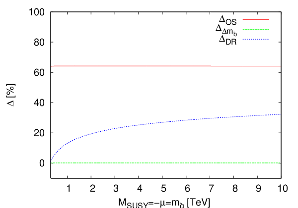
A naive calculation in the OS scheme yields a correction of above $60\%$ . After subtracting the $\Delta m_{b}$ contribution only the real one-loop corrections are left. Their size is of around $0.2\%$ . In the $\overline{\textrm{DR}}$ scheme the corrections are equally small for small mass values and show a logarithmic rise with growing mass. This is an artefact of the mismatch between the renormalization scale and the masses of the squarks and gluinos appearing in the loop diagrams. The former one was fixed to the sum of the final-state particle masses $\mu_{R}=m_{H^{-}}+m_{W}$ . Terms of the order $\ln\frac{M_{SUSY}}{\mu_{R}}$ appear in the expression which originate from the dimensional regularization of the divergent loop integrals. Thus this logarithmic rise bears no physical meaning and will vanish if higher orders of perturbation theory are taken into account.

In the next plot (Fig. 6.5) the squark and gluino masses are now fixed and only $\mu$ is left as a free parameter.

The parameter set for this plot is

$\displaystyle m_{H^{+}}$	$\displaystyle=200\textrm{ GeV}$
$\displaystyle t_{\beta}$	$\displaystyle=30$
$\displaystyle A_{t}$	$\displaystyle=A_{b}=0$
$\displaystyle M_{\tilde{Q}}$	$\displaystyle=M_{\tilde{U}}=M_{\tilde{D}}=500\textrm{ GeV}$
$\displaystyle m_{\tilde{g}}$	$\displaystyle=580\textrm{ GeV}\quad.$	(6.8)

As expected the cross section in the OS scheme grows linearly with $\mu$ . For $\mu$ values less than about $-750\textrm{ GeV}$ the corrections even exceed $100\%$ . Again, when the $\Delta m_{b}$ corrections are subtracted and only the true one-loop SUSY-QCD corrections remain the order of the corrections is below $1\%$ and shows only a very low variation with $\mu$ . In the $\overline{\textrm{DR}}$ scheme the corrections are also much smaller than in the OS scheme and almost constant as a function of $\mu$ , as is expected from the remaining corrections appearing in this scheme.

As next step the dependence of the hadronic cross section differences as a function of $t_{\beta}$ is investigated in Fig. 6.6. Here a data point with a smaller soft-supersymmetry breaking mass is chosen to emphasize the effect which will be discussed below, namely

$\displaystyle m_{H^{+}}$	$\displaystyle=200\textrm{ GeV}$
$\displaystyle\mu$	$\displaystyle=-200\textrm{ GeV}$
$\displaystyle A_{t}$	$\displaystyle=A_{b}=0$
$\displaystyle M_{\tilde{Q}}$	$\displaystyle=M_{\tilde{U}}=M_{\tilde{D}}=200\textrm{ GeV}$
$\displaystyle m_{\tilde{g}}$	$\displaystyle=580\textrm{ GeV}\quad.$	(6.9)

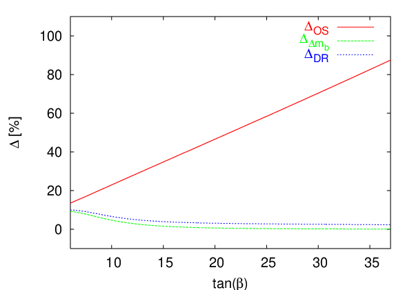
For large values of $t_{\beta}$ the respective corrections feature the behavior which was already observed in the previous plots. The $\Delta m_{b}$ corrections are large, while the true one-loop corrections almost vanish. The corrections in the OS scheme rise linearly with $t_{\beta}$ as is expected from eq. (4.17). For $t_{\beta}\lesssim 15$ however the behavior changes. There the difference between the full one-loop computation and the $\Delta m_{b}$ -corrected tree-level cross section can increase up to $10\%$ . This contribution for small $t_{\beta}$ originates mainly from the diagram given in Fig. 6.7.

The Yukawa coupling of the charged Higgs to the stop and sbottom is proportional to the top-quark mass if a right-handed stop couples to a left-handed sbottom. Another factor $m_{t}$ appears in the trace over the fermion line where for the internal top quark line the mass term in the Dirac algebra is chosen. These two factors cancel the top-quark propagator which is dominated by the mass term and the top-quark mass dependence drops out. To get this left-right mixing term in the Yukawa coupling also the mass term for the gluino appears during the calculation of the fermion trace, giving a factor $m_{\tilde{g}}$ in the nominator. Accordingly this vertex correction to the $tbH^{+}$ vertex is proportional to

\frac{\alpha_{s}}{3\pi}\mu m_{\tilde{g}}I\left(m_{{\tilde{b}}},m_{{\tilde{t}}},m_{\tilde{g}}\right)

(6.10)

where $I$ was given in eq. (4.18) and is related to the three-point integral in the limit of vanishing external momenta. The expression is independent of $t_{\beta}$ . So for small values of $t_{\beta}$ , where the bottom-quark Yukawa coupling is not enhanced, this gives an important contribution. When $t_{\beta}$ takes larger values, the bottom-quark terms dominate. These terms have a factor of $t_{\beta}$ appearing in the amplitude so the cross section increases quadratically with $t_{\beta}^{2}$ . Hence the relative contribution of Fig. 6.7 is reduced. This plot underlines the importance of performing a full one-loop calculation because only in such a full calculation the non-universal corrections are included and a tree-level calculation with effective couplings would give wrong results in the low- $t_{\beta}$ regime.

The variation of the cross section as a function of $\mu$ in the low- $t_{\beta}$ regime is investigated in Fig. 6.8. For this plot $t_{\beta}=6$ was chosen and the other parameters were left unchanged from the last plot. Again the rather small value of $200\textrm{ GeV}$ is chosen for the soft-supersymmetry breaking masses in the squark sector, so that the function $I$ , which is proportional to $\frac{1}{m_{SUSY}^{2}}$ , has a small denominator.

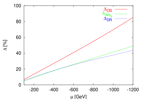
One can clearly see two distinct properties. The one-loop corrections which cannot be absorbed into a redefinition of the bottom-quark Yukawa coupling now give a significant contribution. The $\Delta m_{b}$ corrections still yield an important contribution as can be seen from comparing the $\Delta_{OS}$ and $\Delta_{\Delta m_{b}}$ curves. Yet after subtracting the universal corrections to the bottom-quark Yukawa coupling the remaining non-universal corrections are large. For large values of $\mu$ they can reach more than $50\%$ . They are equally present in the $\overline{\textrm{DR}}$ scheme where a numerical contribution close to the $\Delta m_{b}$ -corrected result is obtained. Furthermore the correction to the cross section increases approximately linearly with the absolute value of $\mu$ as is expected from eq. (6.10).

Furthermore, in Fig. 6.9 a plot where the complete SUSY mass spectrum, i.e. soft-supersymmetry breaking mass terms for the squarks, $\mu$ and the gluino mass, is fixed to the same value and run up to $10\textrm{ TeV}$ is presented for the low- $t_{\beta}$ regime.

The behavior as a function of the mass scale is the same as before in the case of large $t_{\beta}$ . After having subtracted the $\Delta m_{b}$ corrections from the complete one-loop contributions there is still a correction of the order of $10\%$ left which mainly originates from the diagram given in Fig. 6.7. For small mass values the relative correction slightly drops because in this region other diagrams also give a numerically significant contribution.

The scale dependence of the SUSY-QCD corrections is given in Fig. 6.10.

The factorization and renormalization scale of the process are fixed to the same value and varied between 0.1 and 10 times their basic value $\mu_{R}=\mu_{F}=m_{W}+m_{H}$ which is used for the other plots. Even for this large scale variations there is only a mild dependence for the corrections in the OS scheme and the $\Delta m_{b}$ corrections. This is due to the fact that the only scale-dependent parameter is the strong coupling constant $\alpha_{s}$ and the PDFs. On-shell conditions render all other paramaters independent of the scale. In the $\overline{\textrm{DR}}$ scheme also the quark masses are scale dependent resulting in a much larger variation as a function of the scale. Including the Standard-QCD corrections which are already known for this process [150] would reduce this variation, but implementing these additional contributions was beyond the scope of this dissertation.

The last plot in Fig. 6.11 shows the total hadronic cross section as a function of $t_{\beta}$ in both OS and $\overline{\textrm{DR}}$ renormalization schemes. Various cross sections with different contributions taken into account are presented here. The same parameter set as in eq. (6.9) is used for this plot.

${\sigma_{0}}^{\text{OS}}$		Tree-level cross section
${\sigma_{\Delta}}^{\text{OS}}$		$\Delta m_{b}$ -corrected tree-level result
${\sigma_{1}}^{\text{OS}}$		One-loop OS cross section
${\sigma_{\text{full}}}^{\text{OS}}$		One-loop OS cross section including
		resummed higher-order $\Delta m_{b}$ corrections
${\sigma_{1}}^{\text{DR}}$		One-loop $\overline{\textrm{DR}}$ cross section

Table 6.1: Key to the total hadronic cross sections of the process

b\bar{b}\rightarrow H^{+}W^{-}

plotted in Fig. 6.11.

In all cases the total cross section rises quadratically with $t_{\beta}$ in the region where $t_{\beta}$ is larger than about 15. This is the parameter space where the Yukawa coupling to the charged Higgs boson is dominated by the term proportional to the bottom-quark mass, which scales with $t_{\beta}$ , and gives the leading contribution to the cross section. On the left-hand side of the plot, where $t_{\beta}$ is small, in contrast the top-quark mass part is responsible for the overall behavior of the cross section and leads to a decrease with $t_{\beta}$ . In the intermediate region both terms contribute equally much, leading to a minimum of the cross section for $t_{\beta}\approx 8$ .

In total five different cross-section types including miscellaneous contributions are depicted. An overview is given in table 6.1. ${\sigma_{0}}^{\text{OS}}$ , the straight red line, denotes the tree-level contribution in the OS renormalization scheme. The short-dashed blue line, ${\sigma_{0}}^{\text{OS}}$ , is the one-loop cross section in the OS scheme without having used any further effective couplings. ${\sigma_{0}}^{\text{OS}}$ , the long-dashed green line contains the $\Delta m_{b}$ -corrected tree-level result. As seen before in the plots of the relative corrections, this line agrees with the complete one-loop result in the case of large $t_{\beta}$ as in this region only the universal $\Delta m_{b}$ corrections are relevant. In the small- $t_{\beta}$ regime these terms can only account for a part of the total corrections. There are also non-universal terms, mainly coming from the sub-diagram given in Fig. 6.10, which cannot be absorbed into an effective coupling. These ones do not, as observed before, contain any factors of $t_{\beta}$ and hence their effects diminish for higher $t_{\beta}$ values as the total cross section scales with $t_{\beta}^{2}$ . For ${\sigma_{\text{full}}}^{\text{OS}}$ , the dotted pink line, the $\Delta m_{b}$ corrections are included in the resummed version of eq. (4.16). Additionally the non-universal one-loop corrections are added. To avoid double-counting the non-resummed $\Delta m_{b}$ contribution must then be subtracted again, resulting in the following formula

\sigma_{\text{full}}^{OS}=\sigma_{\Delta\text{resum}}^{OS}+\left(\sigma_{1}^{OS}-\sigma_{\Delta}^{OS}\right)\quad.

(6.11)

In this line also phase-space effects from the reduced bottom-quark mass are taken into account, leading to an additional shift with respect to the tree-level cross section. Nevertheless the curve again shows the expected behavior which can be deduced from the results given above with rising corrections for increasing $t_{\beta}$ . For large values of $t_{\beta}$ they largely exceed the one-loop result because of the $\Delta m_{b}$ resummation where contributions are added that in a naive calculation would appear in higher-order diagrams of perturbation theory. This curve presents the current best estimate for the total cross section in the OS scheme where higher-order contributions are included as much as possible. Lastly the one-loop expression in the $\overline{\textrm{DR}}$ scheme is plotted as dash-dotted light-blue line and labeled ${\sigma_{1}}^{\text{DR}}$ . It has a shape very similar to the previous curve because the $\Delta m_{b}$ corrections appear in the self-energy contributions to the bottom-quark mass. In this renormalization scheme they enter completely at one-loop order via the bottom-quark propagators and no further contributions at higher orders appear. Hence this corresponds to the resummed result in the OS scheme. The remaining difference between the two curves is a measure for the theoretical uncertainty of the calculation because of missing non-leading higher-order contributions from perturbation theory.

Finally the numerical results for the parameter point $\text{SPS1a}^{\prime}$ [24] are given in table 6.2. This parameter point is described in appendix A.2, it was chosen as a reference point for MSSM calculations.

Tree-level cross section	$\sigma_{0}$ $=$	$2.684$ fb
$\Delta m_{b}$ -corrected tree-level cross section	$\sigma_{\Delta m_{b}}$ $=$	$2.266$ fb
One-loop OS cross section	$\sigma_{1}$ $=$	2.176 fb
Relative one-loop OS correction	$\Delta_{OS}$ $=$	$-15.6$ %
Relative true one-loop OS correction	$\Delta_{\Delta m_{b}}$ $=$	$-4.0$ %

Table 6.2: Hadronic cross sections for the reference point

\text{SPS1a}^{\prime}

, which is described in appendix A.2.

Because of the positive sign of $\mu$ the one-loop cross section is now reduced with respect to the tree-level result. The $t_{\beta}$ value of $10$ is in a region where the $\Delta m_{b}$ corrections are already the dominant ones, but the non-universal corrections still yield a numerically significant contribution.

Chapter 7 Higgs-Boson Production via Vector Boson Fusion

Proving the existence of a neutral Higgs boson is one of the main tasks of the LHC. Its main production processes for both SM and MSSM Higgs bosons include Higgs-boson production via vector-boson fusion (Fig. 7.1) [153, 155, 156].

Its rate is surpassed only by the gluon-fusion process $gg\rightarrow h^{0}$ [157] shown in Fig. 7.2.

This process has large NLO-QCD corrections with K-factors larger than $2$ [158]. Even after including the NNLO-QCD corrections [161] theoretical uncertainties of $\mathcal{O}\left(10-20\%\right)$ remain. They make the extraction of coupling constants from the gluon-fusion process difficult and lead to large errors.

The Standard-QCD corrections to the vector-boson-fusion process were already calculated before [166, 167]. At tree-level the process only consists of a t-channel exchange of a colorless gauge boson, which is why the contribution where an additional gluon connects the two quark lines has no interference term with the tree-level diagram. Only the quark–anti-quark–vector-boson vertex receives corrections of $\mathcal{O}\left(\alpha_{s}\right)$ and hence the overall QCD corrections are relatively small and typically between $5$ and $10\%$ . Therefore, the extraction of Higgs coupling constants leads to much smaller errors than in the gluon-fusion case, and the vector-boson-fusion production process is, despite its lower cross section, an ideal instrument to study the Higgs boson.

This process possesses a clear experimental signature of two jets in the forward region and thus can be easily separated from background processes by applying appropriate cuts [168]. In this chapter the production of the lightest MSSM Higgs boson $h^{0}$ via vector-boson fusion is investigated and the SUSY-QCD corrections to this process are calculated.

7.1 The Partonic Process

The partonic processes which contribute to the production of a Higgs boson via vector-boson fusion can be summarized in a single general Feynman diagram which is depicted in Fig. 7.1. It can be seen as scattering of two quarks which is mediated via a vector boson in the t-channel with a Higgs boson being radiated off the intermediate vector boson. This is why the process has a clear experimental signature of two jets in the forward region of the detector which allows one to easily distinguish the signal from background processes by using appropriate cuts.

In a strict sense, the general diagram given in Fig. 7.1 is not the only one which contributes to this final state. When a quark–anti-quark pair of the same flavor appears in the initial state they can form a $Zh^{0}$ pair via an intermediate virtual $Z$ boson and the $Z$ subsequently decays again into a quark–anti-quark pair. Hence these diagrams have exactly the same particle content in both the external and internal lines. There are also similar processes where an intermediate $W$ boson can appear in the same way. However, the vector-boson-fusion process has a very distinct signature of two jets in the forward region. Using only this particular phase-space region the interference between the two diagram types is strongly suppressed by the large momentum transfer appearing in the intermediate gauge bosons. Additionally a color suppression factor appears in the interference term [167]. Hence the effects from these additional diagrams can be safely neglected if appropriate cuts [168] to the phase space are applied.

An analysis of the statistical accuracies of the cross section which are achievable at the LHC was done in refs. [169, 171]. It could be shown that a measurement with an accuracy of $5$ to $10\%$ can be performed, also taking uncertainties in the decay branching ratios of the Higgs boson into account. So the size of the NLO-QCD corrections already matches the accuracy which is achievable in experiment. Theoretical uncertainties are not expected to limit the precision with which the cross sections can be measured.

In the MSSM besides the Standard-QCD corrections also SUSY-QCD corrections appear which are of the same order $\mathcal{O}\left(\alpha_{s}\right)$ or, in case of the pentagon diagrams, even enhanced and of $\mathcal{O}\left(\frac{\alpha_{s}^{2}}{\alpha}\right)$ in the coupling constant. A full one-loop calculation of these corrections has not been done before and is presented in this thesis.

7.2 SUSY-QCD Corrections

In this chapter the SUSY-QCD corrections to $h^{0}$ -production via vector-boson fusion are studied. If their size is larger than the experimental uncertainties one might be able to use this to tell the SM and the MSSM apart. In the limit of large $m_{A}$ the couplings of the $h^{0}$ become SM-like. So if at the LHC only one Higgs boson with Standard-Model couplings and a mass below $140\textrm{ GeV}$ is found, the question arises whether a SM or a MSSM Higgs boson was seen in the detector. The SUSY-QCD corrections, which exist only in the case of a MSSM Higgs boson, could modify the Higgs boson coupling by an amount large enough and therefore make the distinction between the two models possible. Also if supersymmetry could be established by other means beforehand, these corrections give an indirect contribution to the coupling between the Higgs boson and two gauge bosons. To be able to extract the value from the experiment as precisely as possible it is necessary to include these higher-order corrections.

The possible types of diagrams which appear in the SUSY-QCD corrections are depicted in Fig. 7.3.

The quark–quark–gauge boson vertices receive corrections which are depicted in Fig. 7.3(a). Their divergencies are cancelled by appropriate counter terms which are shown in Fig. 7.3(b). The contribution of these diagrams was already investigated before [172] for the special case where all squarks have equal mass. Additionally one of the gauge bosons can be replaced by a box-shaped sparticle loop as shown in Fig. 7.3(c). Finally, all external particles can be coupled via a pentagon-type loop as in Fig. 7.3(d). Because of the Majorana nature of the gluinos also the diagram displayed on the right-hand side of the figure, where two quark lines are connected, exists.

All cross sections are calculated in the OS renormalization scheme. For the tree-level diagrams the leading-order parton distribution functions of ref. [173] were used. The one-loop cross sections were convoluted with the NLO-PDFs of the same group given in ref. [174]. In both cases the implementation from the program package LHAPDF [134] was used to obtain the numerical results which are presented in the next section.

7.3 Numerical Results

In this section numerical results for the SUSY-QCD corrections to $h^{0}$ -production via vector-boson fusion are presented. The hadronic cross sections for each individual process for the MSSM reference point $\text{SPS1a}^{\prime}$ , which is described in detail in appendix A.2, are listed in the following table. The one-loop corrections are separated according to the loop type, where $\sigma_{\text{vertex}}$ includes the contributions from the diagrams shown in Fig. 7.3(a) and (b), $\sigma_{\text{box}}$ from the ones of Fig. 7.3(c) and $\sigma_{\text{five-pt.}}$ from the pentagon diagrams depicted in Fig. 7.3(d).

Partonic subprocess	$\sigma_{\text{tree}}$ [pb]	$\frac{\sigma_{\text{vertex}}}{\sigma_{\text{tree}}}$	$\frac{\sigma_{\text{box}}}{\sigma_{\text{tree}}}$	$\frac{\sigma_{\text{five-pt.}}}{\sigma_{\text{tree}}}$
$dd\rightarrow ddh^{0}$	$1.76\cdot 10^{-2}$	$-1.72\cdot 10^{-4}$	$8.34\cdot 10^{-4}$	$1.24\cdot 10^{-5}$
$du\rightarrow duh^{0}$	$3.46\cdot 10^{-1}$	$-1.60\cdot 10^{-4}$	$6.68\cdot 10^{-5}$	$1.46\cdot 10^{-6}$
$ds\rightarrow dsh^{0}$	$1.21\cdot 10^{-2}$	$-1.58\cdot 10^{-4}$	$7.89\cdot 10^{-4}$	$-1.67\cdot 10^{-5}$
$dc\rightarrow dch^{0}$	$6.39\cdot 10^{-3}$	$-1.58\cdot 10^{-4}$	$2.69\cdot 10^{-5}$	$1.83\cdot 10^{-6}$
$dc\rightarrow ush^{0}$	$3.34\cdot 10^{-2}$	$-1.43\cdot 10^{-4}$	$9.07\cdot 10^{-5}$	$0$
$d\bar{d}\rightarrow d\bar{d}h^{0}$	$1.58\cdot 10^{-2}$	$-1.55\cdot 10^{-4}$	$7.77\cdot 10^{-4}$	$2.48\cdot 10^{-6}$
$d\bar{d}\rightarrow u\bar{u}h^{0}$	$6.33\cdot 10^{-2}$	$-1.40\cdot 10^{-4}$	$1.02\cdot 10^{-5}$	$1.52\cdot 10^{-6}$
$d\bar{u}\rightarrow d\bar{u}h^{0}$	$1.09\cdot 10^{-2}$	$-1.53\cdot 10^{-4}$	$2.16\cdot 10^{-5}$	$1.66\cdot 10^{-6}$
$d\bar{s}\rightarrow d\bar{s}h^{0}$	$1.18\cdot 10^{-2}$	$-1.56\cdot 10^{-4}$	$7.83\cdot 10^{-4}$	$-8.90\cdot 10^{-6}$
$d\bar{s}\rightarrow u\bar{c}h^{0}$	$4.75\cdot 10^{-2}$	$-1.41\cdot 10^{-4}$	$1.52\cdot 10^{-5}$	$0$
$d\bar{c}\rightarrow d\bar{c}h^{0}$	$6.26\cdot 10^{-3}$	$-1.56\cdot 10^{-4}$	$2.86\cdot 10^{-5}$	$1.96\cdot 10^{-6}$
$uu\rightarrow uuh^{0}$	$3.68\cdot 10^{-2}$	$-1.86\cdot 10^{-4}$	$-6.65\cdot 10^{-4}$	$-1.26\cdot 10^{-5}$
$us\rightarrow dch^{0}$	$1.10\cdot 10^{-1}$	$-1.49\cdot 10^{-4}$	$8.16\cdot 10^{-5}$	$0$
$us\rightarrow ush^{0}$	$2.12\cdot 10^{-2}$	$-1.65\cdot 10^{-4}$	$1.53\cdot 10^{-4}$	$1.84\cdot 10^{-6}$
$uc\rightarrow uch^{0}$	$1.14\cdot 10^{-2}$	$-1.64\cdot 10^{-4}$	$-6.23\cdot 10^{-4}$	$2.20\cdot 10^{-5}$
$u\bar{d}\rightarrow u\bar{d}h^{0}$	$2.75\cdot 10^{-2}$	$-1.63\cdot 10^{-4}$	$1.56\cdot 10^{-4}$	$1.59\cdot 10^{-6}$
$u\bar{u}\rightarrow d\bar{d}h^{0}$	$1.27\cdot 10^{-1}$	$-1.44\cdot 10^{-4}$	$1.60\cdot 10^{-4}$	$2.00\cdot 10^{-6}$
$u\bar{u}\rightarrow u\bar{u}h^{0}$	$1.92\cdot 10^{-2}$	$-1.61\cdot 10^{-4}$	$-6.05\cdot 10^{-4}$	$-3.15\cdot 10^{-5}$
$u\bar{s}\rightarrow u\bar{s}h^{0}$	$2.08\cdot 10^{-2}$	$-1.64\cdot 10^{-4}$	$1.52\cdot 10^{-4}$	$1.82\cdot 10^{-6}$
$u\bar{c}\rightarrow d\bar{s}h^{0}$	$7.45\cdot 10^{-2}$	$-1.46\cdot 10^{-4}$	$1.56\cdot 10^{-4}$	$0$
$u\bar{c}\rightarrow u\bar{c}h^{0}$	$1.12\cdot 10^{-2}$	$-1.63\cdot 10^{-4}$	$-6.17\cdot 10^{-4}$	$1.77\cdot 10^{-5}$
$ss\rightarrow ssh^{0}$	$8.40\cdot 10^{-4}$	$-1.48\cdot 10^{-4}$	$7.62\cdot 10^{-4}$	$7.40\cdot 10^{-6}$
$sc\rightarrow sch^{0}$	$4.37\cdot 10^{-3}$	$-1.31\cdot 10^{-4}$	$6.04\cdot 10^{-5}$	$1.81\cdot 10^{-6}$
$s\bar{d}\rightarrow s\bar{d}h^{0}$	$2.22\cdot 10^{-3}$	$-1.41\cdot 10^{-4}$	$7.34\cdot 10^{-4}$	$-7.60\cdot 10^{-6}$
$s\bar{d}\rightarrow c\bar{u}h^{0}$	$9.10\cdot 10^{-3}$	$-1.27\cdot 10^{-4}$	$1.93\cdot 10^{-5}$	$0$
$s\bar{u}\rightarrow s\bar{u}h^{0}$	$1.50\cdot 10^{-3}$	$-1.40\cdot 10^{-4}$	$-5.07\cdot 10^{-6}$	$1.72\cdot 10^{-6}$
$s\bar{s}\rightarrow s\bar{s}h^{0}$	$1.62\cdot 10^{-3}$	$-1.42\cdot 10^{-4}$	$7.42\cdot 10^{-4}$	$1.58\cdot 10^{-6}$
$s\bar{s}\rightarrow c\bar{c}h^{0}$	$6.69\cdot 10^{-3}$	$-1.28\cdot 10^{-4}$	$2.33\cdot 10^{-5}$	$3.29\cdot 10^{-8}$
$s\bar{c}\rightarrow s\bar{c}h^{0}$	$8.27\cdot 10^{-4}$	$-1.43\cdot 10^{-4}$	$1.79\cdot 10^{-6}$	$1.96\cdot 10^{-6}$
$cc\rightarrow cch^{0}$	$1.70\cdot 10^{-4}$	$-1.49\cdot 10^{-4}$	$-5.99\cdot 10^{-4}$	$-6.09\cdot 10^{-6}$
$c\bar{d}\rightarrow c\bar{d}h^{0}$	$9.00\cdot 10^{-4}$	$-1.41\cdot 10^{-4}$	$1.88\cdot 10^{-4}$	$1.75\cdot 10^{-6}$
$c\bar{u}\rightarrow s\bar{d}h^{0}$	$4.17\cdot 10^{-3}$	$-1.27\cdot 10^{-4}$	$1.35\cdot 10^{-4}$	$0$
$c\bar{u}\rightarrow c\bar{u}h^{0}$	$6.09\cdot 10^{-4}$	$-1.40\cdot 10^{-4}$	$-5.66\cdot 10^{-4}$	$1.54\cdot 10^{-5}$
$c\bar{s}\rightarrow c\bar{s}h^{0}$	$6.56\cdot 10^{-4}$	$-1.43\cdot 10^{-4}$	$1.85\cdot 10^{-4}$	$1.91\cdot 10^{-6}$
$c\bar{c}\rightarrow s\bar{s}h^{0}$	$2.27\cdot 10^{-3}$	$-1.31\cdot 10^{-4}$	$1.33\cdot 10^{-4}$	$4.08\cdot 10^{-6}$
$c\bar{c}\rightarrow c\bar{c}h^{0}$	$3.31\cdot 10^{-4}$	$-1.44\cdot 10^{-4}$	$-5.84\cdot 10^{-4}$	$-3.33\cdot 10^{-5}$
$\bar{d}\bar{d}\rightarrow\bar{d}\bar{d}h^{0}$	$1.81\cdot 10^{-3}$	$-1.43\cdot 10^{-4}$	$7.32\cdot 10^{-4}$	$7.41\cdot 10^{-6}$
$\bar{d}\bar{u}\rightarrow\bar{d}\bar{u}h^{0}$	$1.36\cdot 10^{-2}$	$-1.28\cdot 10^{-4}$	$5.79\cdot 10^{-5}$	$1.69\cdot 10^{-6}$
$\bar{d}\bar{s}\rightarrow\bar{d}\bar{s}h^{0}$	$2.64\cdot 10^{-3}$	$-1.40\cdot 10^{-4}$	$7.29\cdot 10^{-4}$	$-1.72\cdot 10^{-5}$
$\bar{d}\bar{c}\rightarrow\bar{d}\bar{c}h^{0}$	$1.35\cdot 10^{-3}$	$-1.41\cdot 10^{-4}$	$4.16\cdot 10^{-7}$	$1.73\cdot 10^{-6}$
$\bar{d}\bar{c}\rightarrow\bar{u}\bar{s}h^{0}$	$7.16\cdot 10^{-3}$	$-1.28\cdot 10^{-4}$	$8.44\cdot 10^{-5}$	$0$
$\bar{u}\bar{u}\rightarrow\bar{u}\bar{u}h^{0}$	$7.23\cdot 10^{-4}$	$-1.44\cdot 10^{-4}$	$-5.70\cdot 10^{-4}$	$-6.54\cdot 10^{-6}$
$\bar{u}\bar{s}\rightarrow\bar{d}\bar{c}h^{0}$	$8.30\cdot 10^{-3}$	$-1.31\cdot 10^{-4}$	$7.43\cdot 10^{-5}$	$0$
$\bar{u}\bar{s}\rightarrow\bar{u}\bar{s}h^{0}$	$1.56\cdot 10^{-3}$	$-1.44\cdot 10^{-4}$	$1.76\cdot 10^{-4}$	$1.90\cdot 10^{-6}$
$\bar{u}\bar{c}\rightarrow\bar{u}\bar{c}h^{0}$	$7.90\cdot 10^{-4}$	$-1.45\cdot 10^{-4}$	$-5.81\cdot 10^{-4}$	$2.19\cdot 10^{-5}$
$\bar{s}\bar{s}\rightarrow\bar{s}\bar{s}h^{0}$	$8.40\cdot 10^{-4}$	$-1.49\cdot 10^{-4}$	$7.63\cdot 10^{-4}$	$7.40\cdot 10^{-6}$
$\bar{s}\bar{c}\rightarrow\bar{s}\bar{c}h^{0}$	$4.37\cdot 10^{-3}$	$-1.31\cdot 10^{-4}$	$6.02\cdot 10^{-5}$	$1.81\cdot 10^{-6}$
$\bar{c}\bar{c}\rightarrow\bar{c}\bar{c}h^{0}$	$1.70\cdot 10^{-4}$	$-1.49\cdot 10^{-4}$	$-5.98\cdot 10^{-4}$	$-6.10\cdot 10^{-6}$
$\sum\left(h^{0}\text{ via VBF}\right)$	$1.11\hskip 32.0pt$	$-1.53\cdot 10^{-4}$	$7.69\cdot 10^{-5}$	$3.44\cdot 10^{-7}$

The quoted cross sections are hadronic ones, where the convolution with the PDFs has already been performed. They are given separately for each partonic subprocess to facilitate an easier analysis of the characteristic effects appearing in this process. Additionally the total hadronic cross section is stated, which is the sum of all subprocesses. For some partonic subprocesses no five-point loop diagrams exist at all. In this case the entry in the last column of the table is exactly zero. To exploit the unique characteristics of the final state of this process cuts were used to obtain the cross sections. A lower limit was placed on the transverse momentum $p_{T}$ and the pseudo-rapidity $\eta$ of the outgoing quarks and anti-quarks, so that the final-state jets are clearly separated from the beam pipe, but still in the forward region of the detector. Also a cut on the jet separation $\Delta R$ between each combination of outgoing particles was set to emulate the behavior of the jet-clustering algorithms used in experimental analyses and to be able to resolve the particles in the detector separately. Thus the applied cuts were

\displaystyle p_{T}(q,\bar{q})

\displaystyle\geq 40\textrm{ GeV}

\displaystyle\eta(q,\bar{q})

\displaystyle\geq 2

\displaystyle\Delta R_{qq,q\bar{q},\bar{q}\bar{q},qh^{0},\bar{q}h^{0}}

\displaystyle\geq 0.4\quad.

(7.1)

The formal definition of these quantities was given in chapter 5.4.

There is an interesting observation already at tree-level. The partonic subprocesses which enter via a $Z$ -boson exchange are suppressed with respect to the ones with a $W$ boson as intermediate vector boson. Firstly, the coupling of the $W$ boson to the quarks is enhanced by a factor of $\frac{1}{c_{W}}$ , the inverse of the cosine of the electroweak mixing angle, with respect to the leading term of the $qqZ$ -coupling. Secondly, the $Z$ boson is heavier than the $W$ boson, and the ratio of the two masses is also equal to $\frac{1}{c_{W}}$ . As the gauge-boson propagators are dominated by their mass terms this leads to an additional enhancement of $\frac{1}{c_{W}^{2}}$ for each $W$ boson propagator. So in total the amplitude of a $W$ boson-exchange diagram is enhanced by about $\frac{1}{c_{W}^{6}}$ over one with a $Z$ boson exchange. Accordingly, this amounts to a factor $\frac{1}{c_{W}^{12}}=\frac{1}{{(0.877)}^{12}}\simeq 4.8$ for the tree-level cross section, which corresponds to the observed partonic cross-section ratios. Because of this effect and the large valence-quark densities of the up- and down-quarks in the proton, the partonic subprocess $ud\rightarrow udh^{0}$ gives the leading contribution to the hadronic process.

The vertex corrections all have the same size relative to the respective tree-level cross section and correspond to the results obtained in ref. [172]. Since the coupling of the $W$ boson to the quarks is purely left-handed, they are largest if the off-diagonal elements in the squark mixing matrix are small and therefore left- and right-handed squarks have almost equal masses. Also for the intermediate gluino propagator only the momentum term survives when calculating the trace over the fermion line. It is proportional to the momentum transfer in the t-channel and thus small. For diagrams with $Z$ -boson exchange the situation is more complicated, because the $qqZ$ -coupling contains both left- and right-handed parts. Nevertheless, any subdiagrams involving a mixing of left- and right-handed squarks are proportional to the off-diagonal terms in the squark mixing matrix, which contain the Yukawa coupling of the corresponding quark and are hence small. Hence, the same effects as in the $W$ boson case appear and lead to a similar relative size of the vertex corrections.

In the case of box diagrams the relative size of the corrections shows a much wider range. For some partonic subprocesses they exceed the vertex corrections significantly, which underlines the importance of performing a full one-loop calculation to take all effects into account. Yet for other subprocesses they are much smaller. This is due to the fact that for $W$ -boson exchange large cancellation is manifest. It occurs between the diagrams on the left-hand side of each row of Fig. 7.3(c), where the $h^{0}$ couples to the squark with the flavor of the outgoing quark, and the ones on the right-hand side which have an $h^{0}$ -coupling to the squark with the incoming-quark flavor. Because of the $W$ boson one of the squarks is always up-type and the other one down-type. Their couplings to the $h^{0}$ have a minus sign relative to each other. Any effects from CKM-mixing are neglected, therefore only squarks of the same generation can appear in a single diagram. This is also why only the superpartners of the four light quarks contribute at all. They all have very similar masses, so the absolute value of the $\tilde{q}\tilde{q}W$ -coupling is roughly the same everywhere. Hence the diagrams on the left- and right-hand side of Fig. 7.3(c) almost exactly cancel for $W$ -boson exchange, leading to a strong suppression of this contribution. For $Z$ -boson exchange no such effect occurs and the relative box-diagram contribution is larger by an order of magnitude. Since, as mentioned above, already the tree-level amplitude is smaller for this diagram type, the absolute value of the correction is small as well and these corrections cannot give a significant contribution to the total cross section. Again the correction is maximized in the case where the off-diagonal elements in the squarx mixing matrix are small. Also the change of the coupling constant between tree-level, which is proportional to $s_{\alpha+\beta}$ , to the one-loop one of $s_{\beta-\alpha}$ cannot give an important effect, because the ratio of the two is always above $0.9$ and approaches $1$ in the decoupling scenario, where the additional Higgs bosons of the MSSM are heavy and the $h^{0}$ -coupling becomes SM-like.

For the five-point diagrams a cancellation similar to the box diagrams occurs when the corresponding tree-level process is mediated by a $W$ -boson exchange. Additionally at least twice a left-right mixing term in the squark sector appears in the amplitude. For this reason a term proportional to the Yukawa coupling of the four light quarks enters the expression and leads to a suppression of the one-loop correction. The choice of parameters which yield the biggest one-loop corrections are in this case large terms in the off-diagonal entries of the squark mixing matrices and therefore a larger mass splitting in the squark sector. Additionally for both types the larger masses of the gluinos and squarks, where experimental limits require that they are heavier than the $W$ or $Z$ boson, lead to a further reduction of the cross section. Yet, there is also an enhancement factor. Except for the Higgs coupling, all other four couplings of the pentagon diagrams are proportional to the strong coupling constant, while for the triangular and box-type diagrams two of the couplings are strong and two of them are electroweak. Hence this type of diagram contains an enhancement factor of $\frac{\alpha_{s}}{\alpha}\simeq 14$ . This is however not sufficient to give a significant contribution to the cross section.

7.4 $h^{0}$ -Production with External Gluons

Additionally the production of an $h^{0}$ with one or two gluons in the initial state was considered. The corresponding Feynman diagrams are shown in Fig. 7.4.

Since there is no tree-level coupling of the gluons to the Higgs bosons, these processes occur at the one-loop level in leading order. This leads to an additional factor of $\alpha_{s}$ in the cross section so the total amplitude is of $\mathcal{O}\left(\alpha_{s}^{4}\alpha\right)$ , while the vector-boson-fusion diagram has a factor $\alpha^{3}$ . Given that $\alpha_{s}^{2}$ is of the same numerical size as $\alpha$ these contributions might prove important. Additionally, the gluon densities in the proton are much higher than those of the quarks at typical LHC energies and this further enhances this type of diagram.

The numerical results for these processes with external gluons for the reference point $\text{SPS1a}^{\prime}$ are given in table 7.2.

Partonic subprocess	$\sigma_{\text{one-loop}}$ [pb]
$gd\rightarrow gdh^{0}$	$2.2\cdot 10^{-5}$
$gu\rightarrow guh^{0}$	$1.7\cdot 10^{-5}$
$gs\rightarrow gsh^{0}$	$2.3\cdot 10^{-6}$
$gc\rightarrow gch^{0}$	$9.3\cdot 10^{-7}$
$g\bar{d}\rightarrow g\bar{d}h^{0}$	$3.2\cdot 10^{-6}$
$g\bar{u}\rightarrow g\bar{u}h^{0}$	$2.5\cdot 10^{-6}$
$g\bar{s}\rightarrow g\bar{s}h^{0}$	$2.1\cdot 10^{-6}$
$g\bar{c}\rightarrow g\bar{c}h^{0}$	$8.2\cdot 10^{-7}$
$gg\rightarrow d\bar{d}h^{0}$	$1.8\cdot 10^{-7}$
$gg\rightarrow u\bar{u}h^{0}$	$2.3\cdot 10^{-7}$
$gg\rightarrow s\bar{s}h^{0}$	$2.6\cdot 10^{-7}$
$gg\rightarrow c\bar{c}h^{0}$	$2.5\cdot 10^{-7}$

Table 7.2: One-loop hadronic cross sections for the subprocesses with one or two gluons in the initial state for the MSSM reference point

\text{SPS1a}^{\prime}

In this case the convolution with the PDFs is also already included in the numbers for the cross section. The same cuts as for the vector-boson-fusion process, given in eq. (7.1), were used. Also the same cuts were applied to the final-state gluons as to the quarks and anti-quarks.

Formally this process type constitutes a background to the previously considered process of $h^{0}$ -production via vector-boson fusion. Therefore one wants to pursue the question, how large the total contribution of these diagrams is and if there are cuts which reduce their size with respect to the signal process.

The processes with one gluon in the initial and final state have a momentum distribution similar to the vector-boson-fusion one. The gluon densities in the proton are very large for small $x$ , but rapidly diminish for larger $x$ . In contrast the sea-quark densities fall off much slower and the valence-quark densities have their maximum at about $\frac{1}{6}$ . So the most favorable configuration is the one where the energy to produce the final state mostly originates from the quark. Thus the hadronic center-of-mass frame is strongly boosted with respect to the partonic one, which leads to jets in the forward region of the detector. This would mimic the signature of a vector-boson-fusion process and produce events which cannot be eliminated by cuts. In contrast for processes with two gluons in the initial state the momentum configuration which maximizes the hadronic cross section is the one where both gluons have similar values of $x$ . This leads to more central jets which are suppressed by the applied cuts.

As one can see from the cross sections in table 7.2, the total contribution of these diagrams is of $\mathcal{O}\left(10^{-4}\right)$ and therefore well below the experimental uncertainties, which are in the range of $5$ to $10\%$ . As the total contribution of these background processes is below the statistical uncertainties which can be reached in a measurement of the vector-boson-fusion cross section, these background processes do not affect the experimental determination of the $h^{0}$ -production rate via vector-boson fusion.

Chapter 8 Higgs-Boson Production in Association with Heavy Quarks

The coupling of Higgs bosons to fermions is of the Yukawa type and therefore proportional to the mass of the fermion. The four light quarks, $u$ , $d$ , $s$ and $c$ , all have a mass below or of about $1\textrm{ GeV}$ . This mass should be compared to the Higgs vacuum expectation value $v$ , the scale of electroweak symmetry breaking, to obtain the strength of their respective Yukawa couplings, which are therefore small. In contrast the top-quark mass is of the same order as the electroweak symmetry-breaking scale, making the top-Higgs coupling numerically sizable. The bottom-quark mass of a few GeV also leads to a rather weak coupling to the Higgs boson in the Standard Model. In the MSSM, the coupling to the $h^{0}$ is enhanced by a factor $t_{\beta}$ , so for large values of $t_{\beta}$ its size can become comparable to the top-quark Yukawa coupling. These large Yukawa couplings make Higgs-boson production in association with heavy quarks [175, 178] a phenomenologically interesting process.

In this chapter the production of the lightest CP-even neutral MSSM-Higgs boson $h^{0}$ in association with a bottom or top quark–anti-quark pair is studied. The top quarks decay rapidly into mainly $bW$ and the outgoing bottom quarks can be identified in the detector via $b$ -quark tagging. Therefore both processes form distinct final states which neither interfere with each other nor with the Higgs-boson production via vector-boson fusion presented in chapter 7. First the peculiarities of each of the two processes are discussed separately. Then the one-loop SUSY-QCD corrections for both processes are described. Since the same basic Feynman diagrams appear in both cases, this task is done jointly. The Standard-QCD corrections have already been calculated in refs. [179, 181] for $b\bar{b}h^{0}$ -production and refs. [184, 185, 187] for $t\bar{t}h^{0}$ -production. Finally in the last two sections the numerical results for both processes are shown.

8.1 The $b\bar{b}h^{0}$ Final State

The production of a Higgs boson in association with bottom quarks in the Standard Model was intensively studied in the literature [171, 188, 189].

At tree-level it originates from the annihilation of a quark–anti-quark pair or from a gluon fusion process, where the final-state $b\bar{b}$ -pair is produced via an intermediate gluon, and the Higgs boson radiates off from one of the bottom quarks (Fig. 8.1(a)). Besides these s-channel diagrams the partonic gluon-fusion process also proceeds via a t-channel diagram shown in Fig. 8.1(b), where the Higgs boson can be emitted from both the internal and external bottom-quark lines. The analysis was soon extended [118, 135, 192] to include the lightest MSSM-Higgs boson $h^{0}$ . The diagram types are exactly the same as in the Standard Model case. Only the bottom-quark–Higgs coupling is changed to its supersymmetric counterpart, resulting in

\sigma_{\text{MSSM}}\left(pp\rightarrow b\bar{b}h^{0}\right)=\left(-\frac{s_{\alpha}}{c_{\beta}}\right)^{2}\sigma_{\text{SM}}\left(pp\rightarrow b\bar{b}H\right)\quad,

(8.1)

where $-\frac{s_{\alpha}}{c_{\beta}}$ is the ratio of the bottom-quark coupling to the MSSM $h^{0}$ boson and to the one of the SM Higgs boson $H$ .

The Standard-QCD corrections [179, 181] to this process are also known and reduce the dependence of the cross section on the factorization and renormalization scales.

However, there are subtleties when making a theoretical prediction for total integrated $h^{0}$ -production via this process, i.e. when the final-state bottom quarks are not explicitly detected. In a four-flavor-number scheme, where only gluons and the four light quarks, but no bottom quarks appear in the initial state, large logarithms of $\mathcal{O}\left(\ln{\frac{Q^{2}}{m_{b}^{2}}}\right)$ in the total cross section emerge, where $Q$ is of the order of the Higgs-boson mass. They arise from the kinematical configuration where a gluon splits into a $b\bar{b}$ -pair and the bottom quarks are collinear to the gluon. These logarithms can be resummed using bottom-quark parton densities, thereby using a five-flavor-number scheme. The bottom-quark densities in the proton originate purely from such splitting gluons. So for every bottom quark which appears in a partonic process another bottom (anti-)quark exists in the hadronic final state. This scheme uses the approximation that the outgoing bottom quarks have small transverse momentum and they are assigned zero transverse momentum at leading order. In the five-flavor-number scheme the leading-order partonic process is then $b\bar{b}\rightarrow h^{0}$ . $gg\rightarrow b\bar{b}h^{0}$ only appears at NNLO together with the two-loop corrections to this process [195].

In our case though these large logarithms are avoided by requiring bottom-quark jets with high transverse momenta and a tagging of the final-state bottom quarks in the detector. The additional cuts reduce the cross section by one or two orders of magnitude, but also greatly reduce the background and make this approach more interesting. The existence of bottom-quark jets with large transverse momenta also guarantees that the Higgs boson was emitted from a bottom quark and is therefore proportional to the bottom-quark Yukawa coupling, allowing its precise measurement.

The SUSY-QCD corrections to this process were partly calculated in ref. [196]. There an effective $b\bar{b}h^{0}$ -coupling was used which includes the one-loop squark and gluino contributions, but no box-type or pentagon diagrams were added in their analysis. In this dissertation a full one-loop calculation of the SUSY-QCD corrections is performed.

8.2 The $t\bar{t}h^{0}$ Final State

The production of a Higgs boson in association with a top quark–anti-quark pair [178, 197, 199] proceeds in the same way as the one with a bottom quark–anti-quark pair discussed in the previous section and the same diagrams as in Fig. 8.1 appear. Since the mass of the top quark is of the same order as the electroweak symmetry-breaking scale, its Yukawa coupling gives a sizable contribution and the process is an important channel for Higgs-boson production in the mass region below $125\textrm{ GeV}$ [200]. Furthermore, this process can be used to measure the top-quark Yukawa coupling precisely [202]. The extension of the SM tree-level calculations to the MSSM, where the Higgs boson is an $h^{0}$ , is again straightforward and amounts to a replacement of the Yukawa coupling such that

\sigma_{\text{MSSM}}\left(pp\rightarrow t\bar{t}h^{0}\right)=\left(\frac{c_{\alpha}}{s_{\beta}}\right)^{2}\sigma_{\text{SM}}\left(pp\rightarrow t\bar{t}H\right)\quad,

(8.2)

where $\frac{c_{\alpha}}{s_{\beta}}$ is the ratio of the top-quark coupling to the MSSM $h^{0}$ boson and to the Higgs boson $H$ of the SM. Thus the total cross section in the MSSM is reduced with respect to the SM one by approximately a factor of $\frac{1}{t_{\beta}^{2}}$ .

The Standard-QCD corrections for this process are available in the literature [184, 185, 187]. Their numerical size is of $\mathcal{O}\left(20\%-40\%\right)$ and leads to a stable prediction of total and differential cross sections with respect to variation of the renormalization and factorization scales.

The large mass of the top quark also reduces the size of the collinear logarithms to $\mathcal{O}\left(\ln\frac{Q^{2}}{m_{t}^{2}}\right)$ . Now the argument of the logarithm is close to $1$ . So the higher-order corrections are small and no resummation of these terms needs to be performed. Hence one can safely use the four-flavor-number scheme for this process and need not apply any additional cuts to the final-state top quarks in this case.

A calculation of the SUSY-QCD corrections was performed quite recently in ref. [204]. As the figures of this article include both the Standard-QCD and the SUSY-QCD one-loop contributions a direct comparison of the numerical results is difficult. As far as the principal behavior with respect to a variation of the MSSM parameters is concerned, agreement could be found.

8.3 SUSY-QCD Corrections

In this section the SUSY-QCD corrections to $h^{0}$ -production in association with a heavy quark–anti-quark pair are described. In the Feynman diagrams the heavy quark is denoted by a $Q$ , which represents a $b$ for the bottom-quark and a $t$ for the top-quark final state. Correspondingly, in part of the diagrams the supersymmetric partners to the heavy quark appears, which is marked by $\tilde{Q}$ , specifying $\tilde{b}$ and $\tilde{t}$ , respectively. A small $\tilde{q}$ on the other hand signifies that all squarks can be inserted in the propagator. The $\tilde{q}^{\prime}$ in the $q\bar{q}$ diagrams denotes the superpartner to the initial-state quark.

In Fig. 8.2(a)-(f) the basic types of Feynman diagrams which appear as one-loop SUSY-QCD corrections to $h^{0}$ -production via gluon fusion are depicted. Self-energy corrections (Fig. 8.2(a)) enter either via a squark or gluino loop which is inserted into the intermediate gluon propagator, or a combined squark-gluino two-point loop inserted into the heavy-quark line. In Fig. 8.2(b) the possible vertex corrections are displayed. Squark loops induce an effective gluon-Higgs coupling appearing in the two diagrams on the left-hand side of the first two rows. The diagrams on the right-hand side of the first two rows contain a correction to the coupling between $h^{0}$ and the heavy quark. The third and fourth row feature corrections to the gluon-quark interaction and the last row an additional contribution to the triple-gluon vertex. Diagrams where four particles are connected via a sparticle loop are presented in Fig. 8.2(c). Finally, all five external particles can be joined by a squark-gluino loop as shown in Fig. 8.2(d). The emerging divergences are cancelled by counter-term diagrams shown in Fig. 8.2(e) for the self-energy contributions and (f) for the vertex corrections. All gluon-fusion s-channel diagrams, where the two initial-state gluons couple to a further, intermediate gluon, also exist in the quark–anti-quark–annihilation subprocesses. The only change is the replacement of the two incoming gluons by a quark–anti-quark pair. The additional diagrams which appear for this type of subprocess are depicted in Fig. 8.2(g). They are corrections to the quark–anti-quark–gluon coupling together with the associated counter-term diagram as shown in the first row. Secondly, the coupling of the incoming light quark to the Higgs boson, which is neglected at tree-level, appears at one-loop order as indicated by the diagram in the second row. Finally in the last row the additional box and pentagon diagrams are shown.

In the remaining sections of this chapter the numerical results of $h^{0}$ -production in association with a heavy quark–anti-quark pair are presented. In analogy to chapter 6 several cross-section differences are defined to illustrate the results. All calculations in this chapter were performed in the OS renormalization scheme, so the label indicating the renormalization scheme will in the following be dropped for all items. The relative one-loop correction is defined as

\Delta_{1}=\frac{\sigma_{1}-\sigma_{0}}{\sigma_{0}}\quad,

(8.3)

where $\sigma_{0}$ denotes the tree-level and $\sigma_{1}$ the one-loop cross section. For the calculation of hadronic cross sections the PDF set of ref. [174] was used. Additionally, a $\Delta m_{b,t}$ -corrected tree-level cross section $\sigma_{\Delta}$ was calculated in a similar way as already described in chapter 6, i.e. using the non-resummed version of eq. (4.21) and treating the $\Delta m_{b,t}$ term as a one-loop contribution. Additionally, the contribution to the vertex from the term proportional to the second mixing angle in the MSSM-Higgs sector, $\alpha$ , was included in $\sigma_{\Delta}$ according to eqs. (4.27) and (4.33). The relative correction using only these contributions is defined as

\Delta_{\tilde{0}}=\frac{\sigma_{\Delta}-\sigma_{0}}{\sigma_{0}}\quad.

(8.4)

Finally, the difference between the $\Delta m_{b,t}$ -corrected tree-level cross section and the full one-loop result, which denotes the true one-loop corrections, is given by

\Delta_{\Delta m_{b,t}}=\frac{\sigma_{1}-\sigma_{\Delta}}{\sigma_{0}}\quad.

(8.5)

The renormalization of the strong coupling constant $\alpha_{s}$ was performed as described in chapter 4.2.3.

8.4 Numerical Results for $b\bar{b}h^{0}$

In this section the numerical results for the process $pp\rightarrow b\bar{b}h^{0}$ are presented. First the total hadronic cross section for the MSSM reference point $\text{SPS1a}^{\prime}$ is given in table 8.1.

Partonic subprocess	$\sigma_{0}$ [fb]	$\sigma_{1}$ [fb]	$\Delta_{1}$ [%]	$\Delta_{\tilde{0}}$ [%]
$d\bar{d}\rightarrow b\bar{b}h^{0}$	$0.107$	$0.104$	$-2.48$	$-1.95$
$u\bar{u}\rightarrow b\bar{b}h^{0}$	$0.168$	$0.164$	$-2.56$	$-1.95$
$s\bar{s}\rightarrow b\bar{b}h^{0}$	$0.028$	$0.028$	$-2.26$	$-1.95$
$c\bar{c}\rightarrow b\bar{b}h^{0}$	$0.013$	$0.012$	$-2.20$	$-1.95$
$gg\rightarrow b\bar{b}h^{0}$	$35.647$	$33.734$	$-5.37$	$-1.95$
$\sum\left(pp\rightarrow b\bar{b}h^{0}\right)$	$35.963$	$34.042$	$-5.34$	$-1.95$

Table 8.1: Hadronic cross sections for

b\bar{b}h^{0}

-production at the parameter point

\text{SPS1a}^{\prime}

(see appendix A.2).

It is also given separately for each partonic subprocess. As described before, the outgoing bottom-quark jets are required to have a high transverse momentum, so that large logarithms are avoided and the background processes, where the Higgs boson does not radiate off a bottom quark, are reduced. To this end a cut on the bottom quarks,

p_{T}(b,\bar{b})\geq 20\textrm{ GeV}\quad,

(8.6)

was applied to obtain these results. The same cut will also be used for all other cross sections of this section.

As one can see in the table, the dominant contribution originates from the gluon-fusion process and the quark–anti-quark–annihilation processes are suppressed by two orders of magnitude. Hence their contribution is negligible and in the following analysis only the gluon-fusion subprocess is considered. This large difference in the cross sections is due to the fact that the quark–anti-quark–annihilation process can only proceed via the s-channel diagram shown on the left-hand side of Fig. 8.1(a). It contains a propagator suppression from the intermediate gluon which must carry at least the energy to procuce the final-state Higgs boson and the two bottom quarks. In contrast the gluon-fusion subprocess also contains a t-channel diagram (Fig. 8.1(b)) which does not suffer from such a suppression. In fact, if one takes only the s-channel diagram on the right-hand side of Fig. 8.1(a) into account, the cross section of the gluon-fusion contribution is of comparable size $(\sigma_{1}=1.103\text{ fb})$ to the one of quark–anti-quark annihilation.

In the following plots the effect of varying MSSM parameters on the SUSY-QCD contributions is investigated. To that end a parameter point with a fairly light SUSY spectrum was chosen, namely

$\displaystyle m_{A}$	$\displaystyle=200\textrm{ GeV}$
$\displaystyle\mu$	$\displaystyle=300\textrm{ GeV}$
$\displaystyle A_{t}$	$\displaystyle=A_{b}=0$
$\displaystyle M_{\text{SUSY}}$	$\displaystyle\equiv M_{\tilde{Q}}=M_{\tilde{U}}=M_{\tilde{D}}=250\textrm{ GeV}$
$\displaystyle m_{\tilde{g}}$	$\displaystyle=400\textrm{ GeV}\quad.$	(8.7)

The MSSM parameters were then varied around this point. The renormalization scale, which appears in $\alpha_{s}$ (see eq. (4.9)), was set to $\mu_{R}=2m_{b}+m_{h^{0}}$ . As the contribution of the quark–anti-quark annihilation diagrams is negligible compared to the gluon-fusion subprocess, only the latter one is considered in the following. Also for simplicity the quoted cross section differences are partonic ones with a center-of-mass energy of $\sqrt{\hat{s}}=500\textrm{ GeV}$ .

For the first plots $t_{\beta}$ is set to the large value $30$ . In the plot given in Fig. 8.3 a common mass scale $M_{\text{SUSY}}$ , where all soft-supersymmetry breaking masses in the squark sector take the same value, is chosen.

According to chapter 4.3, where the bottom-quark Yukawa coupling was studied, one would expect the universal corrections, which are parametrized in $\Delta m_{b}$ , to give the dominant contribution. This is indeed the case for almost all $M_{\text{SUSY}}$ -values. Also the decrease of the corrections with growing SUSY mass scale, which is predicted by eq. (4.17) to fall off as $\frac{1}{M_{\text{SUSY}}^{2}}$ , can be seen in the plot. Only for rather small values of $M_{\text{SUSY}}$ a deviation from this behavior occurs. Other terms contribute significantly in this region and lead to smaller cross-section differences than one would expect from the $\Delta m_{b}$ terms alone.

The numbers for the second plot (Fig. 8.4) are also calculated in the regime of large $t_{\beta}$ , but now $\mu$ is varied.

For small values of $\mu$ , the $\Delta m_{b}$ -corrected tree-level result and the full one-loop cross section coincide and show the expected linear rise with $\mu$ . When $\mu$ becomes large, and thus the off-diagonal elements in the sbottom mixing matrix lead to a larger split between the lighter and heavier sbottom, this behavior changes and leads to a decelerated increase with $\mu$ . Also other terms begin to contribute to the cross section in a significant way and induce a deviation of the full one-loop result from the $\Delta m_{b}$ corrections by up to $20\%$ .

The effect of varying $t_{\beta}$ is studied in Fig. 8.5.

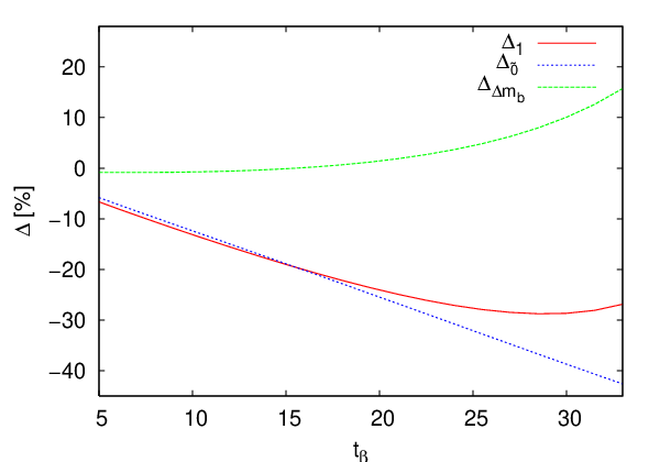
The $\Delta m_{b}$ -corrected tree-level result grows linearly with $t_{\beta}$ as predicted from eq. (4.17). In the small $t_{\beta}$ -regime it approximates the full one-loop result rather well with a deviation of only about one percent. For larger values of $t_{\beta}$ the complete one-loop corrections begin to deviate and additional contributions lead to a slower rise. Finally, the absolute value of the full corrections slightly decreases again. This is the same effect which was already observed on the left-hand side of Fig. 8.3. As the common value of the soft supersymmetry-breaking masses $M_{\text{SUSY}}$ was chosen to be $250\textrm{ GeV}$ we are exactly in this regime. A higher value for $M_{\text{SUSY}}$ leads to a one-loop cross-section difference which coincides with the $\Delta m_{b}$ -corrected tree-level one over the whole range of $t_{\beta}$ . To verify this a value of $M_{\text{SUSY}}=400\textrm{ GeV}$ was chosen to obtain Fig. 8.6. Additionally, the gluino mass was set to $m_{\tilde{g}}=640\textrm{ GeV}$ such that the ratio of the two masses is the same as in the parameter set eq. (8.7).

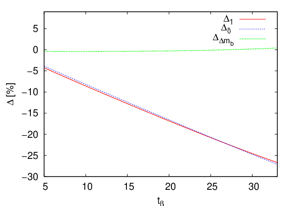
In this case the discrepancy $\Delta_{\Delta m_{b}}$ between $\Delta_{1}$ and $\Delta_{\tilde{0}}$ stays below one percent for all $t_{\beta}$ -values.

In the final two plots the behavior of the cross-section differences in the small $t_{\beta}$ -regime, namely for $t_{\beta}=6$ , is studied. Firstly, in Fig. 8.7 the common mass scale $M_{\text{SUSY}}$ of the soft supersymmetry-breaking masses appearing in the squark sector is varied.

The $\Delta m_{b}$ -corrected tree-level result is a good approximation of the full one-loop result over the whole mass range. The difference is about one percent for small $M_{\text{SUSY}}$ and rapidly vanishes for larger values.

The last plot (Fig. 8.8) depicts the dependence of the cross-section differences on $\mu$ for $t_{\beta}=6$ .

It shows a similar behavior as the same plot for large $t_{\beta}$ (Fig. 8.4). For small values of $\mu$ the $\Delta m_{b}$ -corrected tree-level result and the full one-loop calculation coincide, while for larger ones significant deviations occur. In the small $t_{\beta}$ -regime the absolute value of the $\Delta_{\tilde{0}}$ corrections even grows slightly larger than the linear behavior of eq. (4.17), which is due to additional effects originating from the growing mass splitting between the two sbottoms. The one-loop corrections in contrast decrease again, once the absolute value has reached a maximum at about $1500\textrm{ GeV}$ , and even change sign and become positive. So in this parameter region true one-loop corrections contribute significantly.

8.5 Numerical Results for $t\bar{t}h^{0}$

The numerical results for the second process of Higgs production in association with heavy quarks, $pp\rightarrow t\bar{t}h^{0}$ , are presented in this section. In table 8.2 the hadronic cross section for the MSSM reference point $\text{SPS1a}^{\prime}$ is denoted. It is given separately for each partonic subprocess which contributes to the $t\bar{t}h^{0}$ -final state.

Partonic subprocess	$\sigma_{0}$ [fb]	$\sigma_{1}$ [fb]	$\Delta_{1}$ [%]
$d\bar{d}\rightarrow t\bar{t}h^{0}$	$42.7$	$37.6$	$-11.77$
$u\bar{u}\rightarrow t\bar{t}h^{0}$	$71.9$	$63.4$	$-11.81$
$s\bar{s}\rightarrow t\bar{t}h^{0}$	$7.5$	$6.6$	$-11.58$
$c\bar{c}\rightarrow t\bar{t}h^{0}$	$2.8$	$2.5$	$-11.53$
$gg\rightarrow t\bar{t}h^{0}$	$273.7$	$264.7$	$-3.30$
$\sum\left(pp\rightarrow t\bar{t}h^{0}\right)$	$399.0$	$374.8$	$-5.96$

Table 8.2: Hadronic cross sections for

t\bar{t}h^{0}

-production at the parameter point

\text{SPS1a}^{\prime}

, which is defined in appendix A.2.

In this case the quark–anti-quark annihilation diagrams give a contribution which is of comparable size to the gluon-fusion ones. On the partonic level the same analysis as in the previous section for $h^{0}$ -production in association with a bottom quark–anti-quark pair holds. The quark–anti-quark–annihilation processes are suppressed because there only a propagator-suppressed s-channel diagram exists, while the gluon-fusion subprocess also proceeds via a t-channel diagram which does not suffer from such a suppression. After the convolution with the parton distribution functions the situation however changes. The gluon densities in the proton show a much steeper fall with growing parton-momentum fraction $x$ than the sea-quark ones. As the top quarks are much heavier than the bottom quarks, also the energy and thus the $x$ of the incoming partons must be larger to be above the threshold for $t\bar{t}h^{0}$ -production. For this final state it approximately compensates the effect from the propagator suppression. The gluon-fusion process is still the dominant production mode, but all processes need to be taken into account for a complete analysis.

In the following plots the effect of varying MSSM parameters on the SUSY-QCD contributions is investigated. To that end the same parameter point as in the previous section with a fairly light SUSY spectrum was chosen, namely

$\displaystyle m_{A}$	$\displaystyle=200\textrm{ GeV}$
$\displaystyle t_{\beta}$	$\displaystyle=6$
$\displaystyle\mu$	$\displaystyle=300\textrm{ GeV}$
$\displaystyle A_{t}$	$\displaystyle=A_{b}=0$
$\displaystyle M_{\tilde{Q}}$	$\displaystyle=M_{\tilde{U}}=M_{\tilde{D}}=250\textrm{ GeV}$
$\displaystyle m_{\tilde{g}}$	$\displaystyle=400\textrm{ GeV}\quad.$	(8.8)

The MSSM parameters were then varied around this point. $t_{\beta}=6$ was kept fixed for all plots of this section. The renormalization scale, which enters $\alpha_{s}$ via eq. (4.9), and the factorization scale were set to $\mu_{R}=\mu_{F}=2m_{t}+m_{h^{0}}$ . The hadronic cross-section calculations were performed for the LHC with a proton-proton center-of-mass energy of $14\textrm{ TeV}$ .

First a common mass scale $M_{\text{SUSY}}$ , where the soft supersymmetry-breaking squark mass terms all take the same value, is introduced and varied between $200$ and $2000\textrm{ GeV}$ , as shown in Fig. 8.9.

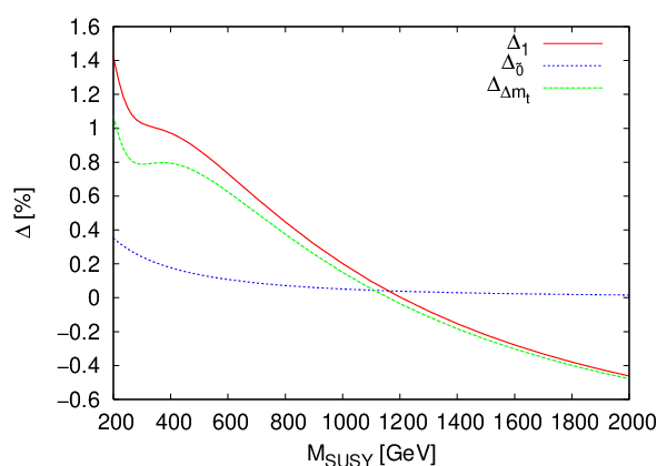
The difference between the tree-level cross section and the $\Delta m_{t}$ -corrected one falls off as $\frac{1}{M_{\text{SUSY}}^{2}}$ , as expected from the form of the $\Delta m_{t}$ term given in eq. (4.30). The total one-loop contributions show a similar decrease, but with a larger coefficient which leads to a much steeper descent. This originates from the fact that the $\Delta m_{t}$ term only includes vertex corrections to the $t\bar{t}h^{0}$ vertex. Yet there are many other one-loop diagrams which also contribute and lead to the modified behavior. In contrast to $\Delta m_{b}$ , which is enhanced by a factor $t_{\beta}$ , the $\Delta m_{t}$ corrections are suppressed by $\frac{1}{t_{\beta}}$ and their numerical effect is expected to be smaller. For small SUSY masses threshold effects of the squark masses induce a deviation from the scaling with $\frac{1}{M_{\text{SUSY}}^{2}}$ .

In the second plot (Fig. 8.10) the dependence of the relative corrections on $\mu$ , the mass parameter mixing the two Higgs doublets, is presented.

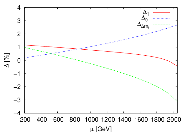
Also in this case the $\Delta m_{t}$ -corrected tree-level cross section is not a good approximation. Whereas the term rises with growing $\mu$ , the full one-loop correction decreases in this case. The slope is constant over a large range of $\mu$ . Only for bigger values, when the off-diagonal entries in the squark mixing matrices become very large and yield an additional contribution, also the gradient increases.

Finally, in Fig. 8.11 $t_{\beta}$ is varied.

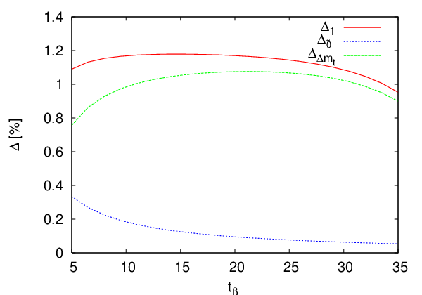
The corrections to the $\Delta m_{t}$ -corrected tree-level result fall off with growing $t_{\beta}$ . This is again the expected behavior of eq. (4.30). The full one-loop corrections are significantly larger in size. They show a mild dependence on this parameter, with a maximum at around $t_{\beta}=15$ .

Chapter 9 Quartic Higgs Coupling at Hadron Colliders

In this chapter another possibility is investigated to test the means of electroweak symmetry breaking. This is achieved by measuring the quartic Higgs coupling and hence fully determining the Higgs potential [34].

After the discovery of a light Higgs boson the next step will be to study its properties, including its couplings to other particles. At the planned International Linear Collider (ILC) measuring these couplings with high precision will be possible for all Standard Model bosons and fermions [205]. Furthermore, if supersymmetric particles are found, the coupling of the Higgs to charginos and neutralinos can be measured precisely [206]. To fully understand electroweak symmetry breaking it is important to measure the Higgs self-couplings and to thereby determine the parameters of the Higgs potential.

9.1 Higgs potential

The Higgs potential of the Standard Model was already given in eq. (2.2). In this model the trilinear ( $\lambda_{3}$ ) and quartic ( $\lambda_{4}$ ) Higgs self-coupling are related to the Higgs mass via

\displaystyle\lambda_{3}=

\displaystyle\frac{-3im_{H}^{2}}{v}

\displaystyle\lambda_{4}=

\displaystyle\frac{-3im_{H}^{2}}{v^{2}}=\frac{\lambda_{3}}{v},

(9.1)

where $v$ is the vacuum expectation value of the Higgs field.

In models with more than one Higgs field, like the MSSM with its two fundamental Higgs doublets, the relations between the trilinear and quartic Higgs coupling can change significantly. For the lighter CP-even MSSM Higgs boson $h^{0}$ the ratio of the self-couplings is

\frac{\lambda_{3h^{0}}}{\lambda_{4h^{0}}}=v\frac{s_{\beta+\alpha}}{c_{2\alpha}},

(9.2)

where $v=\sqrt{v_{1}^{2}+v_{2}^{2}}$ and $v_{1}$ and $v_{2}$ are the vacuum expectation values of the two Higgs fields. If the parameter $m_{A}$ is sufficiently large there is a mass splitting between $h^{0}$ and the remaining Higgs sector. Additionally, the angles $\alpha$ and $\beta$ are related via $s_{\alpha}\simeq-c_{\beta}$ in this limit. Therefore $\frac{s_{\beta+\alpha}}{c_{2\alpha}}$ approaches $1$ and the $h^{0}$ -coupling becomes Standard Model-like.

In this chapter we will not refer to the MSSM as our underlying theory. Instead we use an effective theory whose particle content is the same as the one of the Standard Model. Its Higgs sector also contains one doublet but the trilinear and quartic couplings are left as free parameters of the theory. In this way we are not restricted on a specific model but can accommodate for many different ones. Such deviations from the Standard Model couplings can for example be generated when higher-dimensional powers of the Higgs doublet are added to the potential as shown in chapter 2.2.2. Taking the first two higher-order terms into account the Higgs self-couplings become

	$\displaystyle\lambda_{3}=$	$\displaystyle\lambda_{3}\left(1+\frac{{\tilde{\lambda}}_{1}v^{2}}{{\tilde{\lambda}}_{0}\Lambda^{2}}\right)$
	$\displaystyle\lambda_{4}=$	$\displaystyle\lambda_{4}\left(1+\frac{6{\tilde{\lambda}}_{1}v^{2}}{{\tilde{\lambda}}_{0}\Lambda^{2}}+\frac{4{\tilde{\lambda}}_{2}v^{4}}{{\tilde{\lambda}}_{0}\Lambda^{4}}\right)\quad.$		(9.3)

The additional terms are suppressed by $\Lambda$ which is the scale where new physics sets in. Both self-couplings receive different contributions from the additional terms. In general, the self-couplings may even become negative. The stability of the Higgs potential is guaranteed if the highest non-vanishing term in the potential has a positive sign. All other terms can have arbitrary values as long as the ground state has a non-vanishing vacuum expectation value to break the electroweak symmetry.

9.2 Trilinear Higgs coupling

As we will see below it is essential for the measurement of the quartic Higgs coupling to know the value of the trilinear Higgs coupling as precisely as possible. For a Higgs boson with a mass larger than $150\textrm{ GeV}$ this coupling can be extracted at the LHC [207, 209, 213]. At least two Higgs bosons must be produced to measure the three-Higgs coupling. At hadron colliders this is performed via a gluon fusion process. In this process two distinct types of diagrams appear, as shown in Fig. 9.1.

Either (a) an intermediate Higgs boson is produced via a three-point top-quark loop diagram which couples to the two final-state Higgs bosons and contains the required trilinear coupling, or (b) the particles couple via a four-point box-type top-quark loop. For the detection of the Higgs bosons the decay channel into two $W^{+}W^{-}$ boson pairs is analyzed [213]. Two or three of the four $W$ bosons are required to decay leptonically into a lepton and a neutrino to have a clear detector signal and the other two or one, respectively, decay hadronically into two jets.

Additional information can be obtained from the kinematic distributions of the Higgs bosons. Not only the total cross section carries information on the trilinear Higgs coupling but also the differential hadronic distribution with respect to the invariant mass of the final state. This can only be calculated correctly if the top-quark loop is fully taken into account. Using the infinite top-quark mass limit and an effective gluon-gluon-Higgs coupling will yield completely incorrect results, as was shown in ref. [213].

Using this information it was evaluated [213] with which precision the trilinear Higgs coupling for Higgs bosons heavier than $150\textrm{ GeV}$ can be measured. In the beginning of LHC a non-zero value can be established with a confidence level of $95\%$ after having accumulated a luminosity of $300~\text{fb}^{-1}$ . After a luminosity upgrade the self-coupling can be measured with a precision of up to $20\%$ at the $95\%$ confidence level using an integrated luminosity of $3~\text{ab}^{-1}$ . At a future high-energy Very Large Hadron Collider (VLHC) with a hadronic center-of-mass energy of $200\textrm{ GeV}$ , the measurement of $\lambda_{3}$ can be performed with an uncertainty of about $10\%$ at a confidence level of $95\%$ after having accumulated a luminosity of $1~\text{ab}^{-1}$ .

In contrast a linear collider can measure the three-Higgs coupling for small Higgs masses of around $120\textrm{ GeV}$ , but possibly not for higher ones [217, 218]. The mass region below $140\textrm{ GeV}$ is more difficult for hadron colliders, because the dominant decay mode for the Higgs boson is a bottom quark–anti-quark pair which has large QCD backgrounds. Anyway, it is still accessible using rare decays [225]. The creation of the two Higgs bosons at an $e^{+}e^{-}$ linear collider happens as double-Higgs strahlung in association with a $Z$ boson or as $WW$ double-Higgs fusion in association with a $\bar{\nu}\nu$ -pair as shown in Fig. 9.2 and Fig. 9.3, respectively.

For a Higgs mass of $120\textrm{ GeV}$ the planned International Linear Collider (ILC) with a center-of-mass energy of $500\textrm{ GeV}$ will be able to measure the trilinear Higgs coupling with an accuracy of $20\%$ within one standard deviation after having accumulated a luminosity of $1~\text{ab}^{-1}$ . A proposed Compact Linear Collider (CLIC) with a center-of-mass energy of $3\textrm{ TeV}$ finally could measure a $180\textrm{ GeV}$ Higgs boson with a precision of $8\%$ within one standard deviation using $5~\text{ab}^{-1}$ of integrated luminosity.

In general the proposed future generation of hadron (VLHC) and linear (CLIC) colliders will be able to measure the trilinear Higgs coupling with an accuracy of $\mathcal{O}\left(10\%\right)$ . A combination of both collider types thereby covers the whole mass range where a Standard Model Higgs boson is expected to be found, as derived from electroweak precision analyses [30].

9.3 Quartic Higgs coupling

As the production of two Higgs bosons is needed for measuring the trilinear Higgs coupling, three final-state Higgs bosons are necessary for a measurement of the quartic Higgs coupling.

Three-Higgs production at linear colliders has already been studied in ref. [226]. It was found that even at CLIC the cross section is too low, with only about five three-Higgs events per year being produced there at a center-of-mass energy of $10\textrm{ TeV}$ . Hence it will be impossible to determine the quartic Higgs coupling at the next generations of linear colliders.

At hadron colliders the three Higgs bosons are dominantly produced via gluon fusion and an intermediate top-quark loop, like in the two-Higgs case. Four distinct topologies appear as shown in Fig. 9.4: (a) continuum production of three Higgs bosons via a five-point top-quark loop, (b) production of two Higgs bosons via a box-type loop and subsequent decay of one of the Higgs bosons via the trilinear self-coupling into two Higgs bosons, and finally the production of one intermediate Higgs boson via a three-point loop. This can either (c) decay via a chain of two three-Higgs couplings or (d) through one quartic Higgs coupling. Only the last diagram type contains the coupling we want to measure.

Looking at the diagrams it is clear that a precise knowledge of the trilinear self-coupling is necessary to obtain results on the quartic self-coupling. The process is also very sensitive to the top-quark Yukawa coupling which must be known very well. In the numerical analysis we have also included the diagrams where the top-quark loops are replaced by bottom-quark loops. The contribution of these diagrams is however less than one percent.

The total cross section as function of the Higgs mass is shown in Fig. 9.5 for the (a) LHC and a (b) $200\textrm{ TeV}$ VLHC.

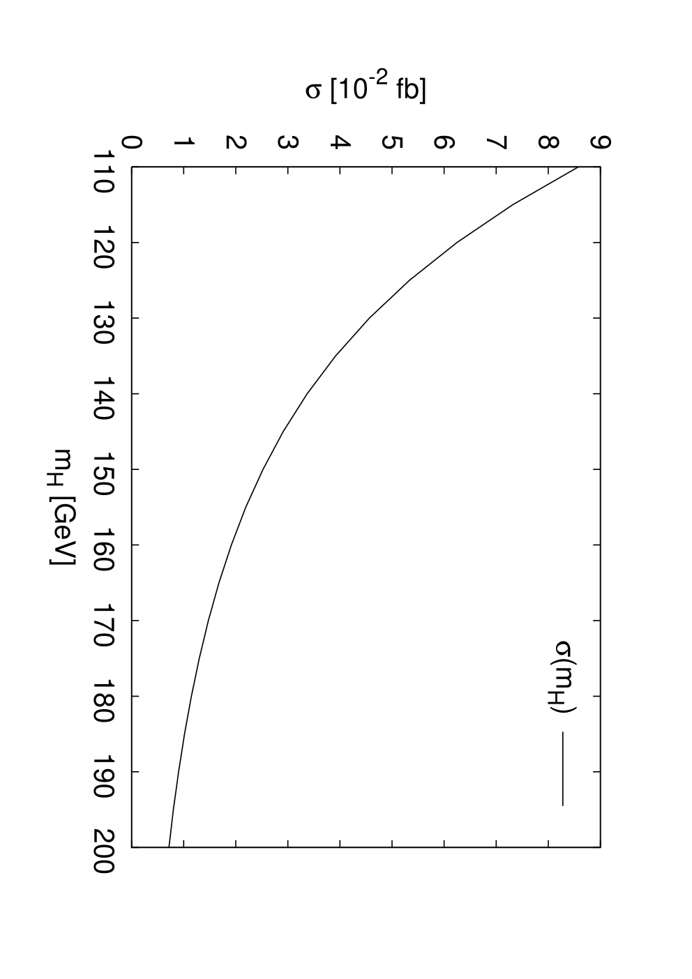
In the following the Higgs boson mass is set to $120\textrm{ GeV}$ for all cross sections and plots.

In Fig. 9.6 the dependence of the total cross section on the trilinear and quartic Higgs coupling is shown.

The values of the trilinear and quartic self-couplings are varied between minus and plus two times the Standard Model value. One can clearly see the strong dependence on $\lambda_{3}$ . The variation on $\lambda_{4}$ is much smaller, as one can see in more detail in Fig. 9.7.

For positive values of $\lambda_{3}$ and $\lambda_{4}$ the variation of the cross section stays below $20\%$ at both the LHC and the VLHC. Including negative values of $\lambda_{4}$ induces changes in the cross section of up to a factor 2. For negative values of $\lambda_{3}$ the absolute variation as a function of $\lambda_{4}$ stays at the same order of magnitude. While the total cross section depends strongly on $\lambda_{3}$ , the relative variation with $\lambda_{4}$ is heavily suppressed.

As the quartic Higgs coupling contributes only to the single diagram Fig. 9.4(d) this behavior is expected. It is also reflected in the partial contributions from the different diagram types. Taking into account all diagrams leads to a Standard Model cross section of $6.25\cdot 10^{-2}~\text{fb}$ at the LHC. Using Standard Model couplings the five-(Fig. 9.4(a)), four-(Fig. 9.4(b)) and three-point(Fig. 9.4(c,d)) loop diagrams alone yield a cross section of $(17.07,8.20,0.46)\cdot 10^{-2}~\text{fb}$ , respectively. The small size of the triangle-type diagram results from a suppression factor by the intermediate Higgs propagator. If one only takes this diagram type into account and sets either $\lambda_{4}$ or $\lambda_{3}$ to zero, a cross section of $0.17~\cdot 10^{-2}~\text{fb}$ from the trilinear self-coupling and of $0.08\cdot 10^{-2}~\text{fb}$ from the quartic self-coupling is obtained. For the VLHC the partial cross sections have similar ratios. So the diagram which contains the quartic self-coupling is almost two orders of magnitude smaller than the total cross section.

As one would expect from the evaluation of the trilinear Higgs coupling in two-Higgs production [213] the interference between the pentagon and the box diagrams is indeed destructive for positive values of $\lambda_{3}$ . This results in the large increase of the cross section when $\lambda_{3}$ gets smaller and therefore the contribution from the box diagram diminishes as one can see in Fig. 9.6. For negative values of $\lambda_{3}$ the single three-Higgs vertex in the box diagrams changes sign and therefore makes this interference constructive, leading to the sharp rise of the cross section. The trilinear and pentagon diagrams interfere constructively, but because the triangle and box contributions have a more similar kinematic configuration, the destructive interference between those two results in a slight decrease of the cross section with growing $\lambda_{4}$ . Only for $\lambda_{3}=0$ , where the box diagrams do not contribute any longer, the behavior of the cross section reverses and rises with increasing $\lambda_{4}$ . The relative signs of the different topologies can be understood analytically by using the low-energy theorem for the leading form factors [227]. An expansion is performed in the ratio $\tfrac{m_{H}}{m_{t}}$ with a partonic center of mass energy $\hat{s}\sim m_{h}^{2}$ . The top-quark mass and the top-quark Yukawa coupling are both denoted by $m_{t}$ . These form factors are basically the squared matrix element without any couplings or additional propagators which are not part of the loop integral. They are obtained starting from the top loop in the gluon self-energy. An additional Higgs boson can be attached to the loop by using the following recursion relation:

F_{(n+1)H}=m_{t}^{2}\frac{\partial}{\partial m_{t}}\frac{F_{nH}}{m_{t}}\quad.

(9.4)

This relation yields

F_{\text{pentagon}}=-F_{\text{box}}=F_{\text{triangle}}=\frac{2}{3}+\mathcal{O}\left(\frac{m_{H}^{2}}{m_{t}^{2}}\right)\quad.

(9.5)

Therefore the structure of constructive and destructive interferences in the diagram types is explained by the relative minus sign in front of the box-type term.

In the case of two-Higgs production the information on the value of $\lambda_{3}$ was not only encoded in the total cross section. Also the differential hadronic cross section with respect to the invariant mass carries information on $\lambda_{3}$ . The same is true for three-Higgs production. In Fig. 9.8 the normalized cross section as a function of the partonic center-of-mass energy is shown.

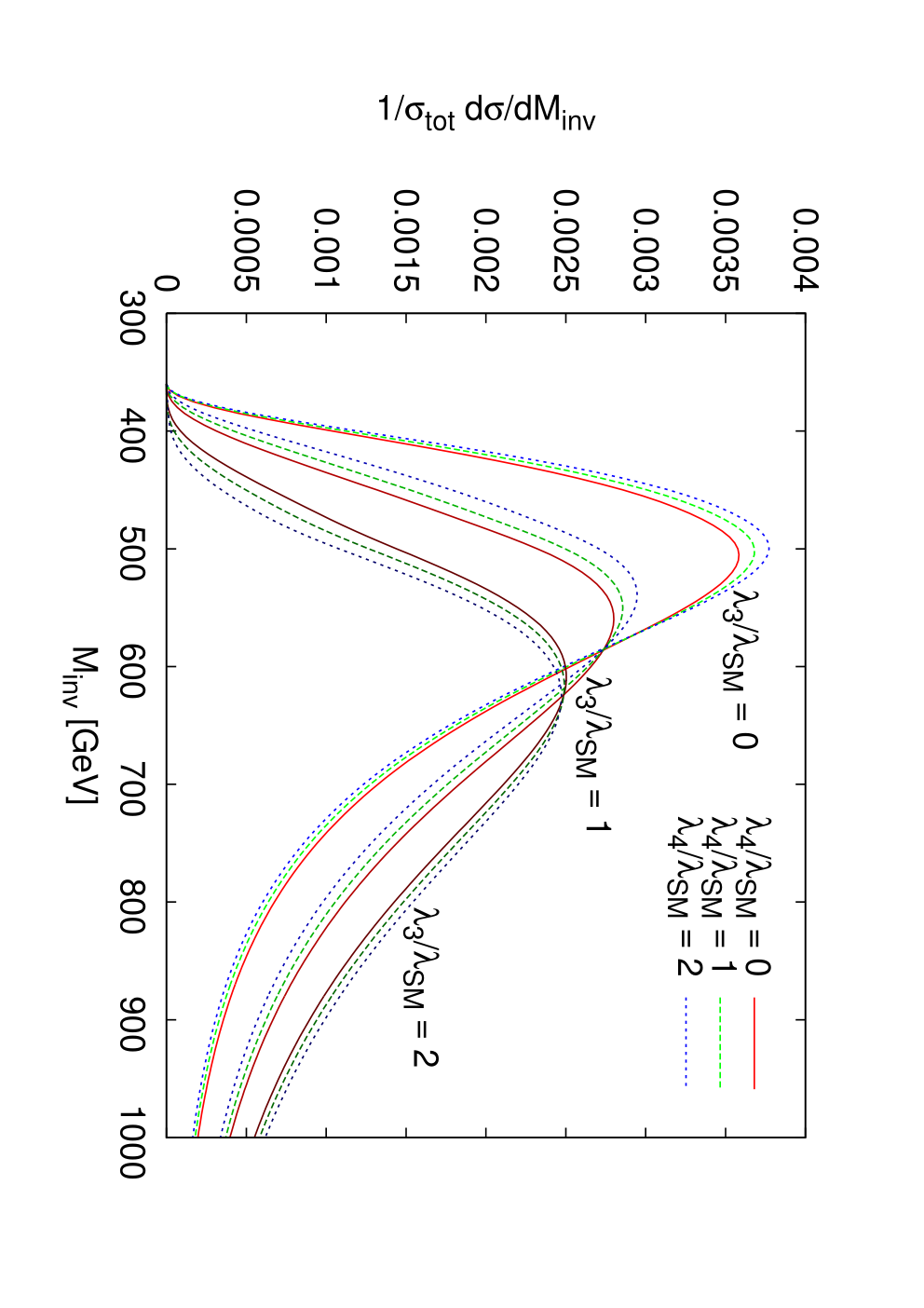
The trilinear and quartic self-coupling both take the values $0$ , $1$ and $2$ times their respective Standard Model value. When varying $\lambda_{3}$ the position of the peak changes significantly and an extraction of this coupling is possible, as was already found in the analysis of two-Higgs production [213]. When changing $\lambda_{4}$ , and keeping $\lambda_{3}$ constant, the size of the shift is about an order of magnitude smaller. Additionally for $\lambda_{3}=0$ the order of the $\lambda_{4}/\lambda_{\text{SM}}=0,1,2$ peaks is inverted which is due to the different sign in the interference as explained above.

The total hadronic cross section for triple-Higgs production via gluon fusion using Standard Model Higgs self-couplings is $6.25\cdot 10^{-2}~\text{fb}$ at the LHC for a Higgs boson with a mass of $120\textrm{ GeV}$ . This rate is too low to be measurable even for the high-luminosity mode of the LHC. At the VLHC with a center-of-mass energy of $200\textrm{ GeV}$ the cross section is $9.45~\text{fb}$ so three-Higgs production might be observable at this future collider. The rather strong dependence of the total cross section on $\lambda_{3}$ , especially for values smaller than the Standard Model value, allows to extract the value of this coupling, thereby possibly confirming the two-Higgs production result. The variation in $\lambda_{4}$ is much smaller, typically below $20\%$ . Hence the extraction of this coupling is much harder. If one takes into account the theoretical uncertainties from missing higher-order corrections and the experimental error on the measurements of $\lambda_{3}$ and the top-quark mass, the chances to be able to extract the quartic Higgs coupling are tiny.

Also in the differential cross section there is a clear effect on the peak position when varying $\lambda_{3}$ . This shift will be the mode to extract the trilinear coupling in double-Higgs production. The size of the shift for a variation of $\lambda_{4}$ is much smaller. If the errors on the measurements of $\lambda_{3}$ and the top-quark mass are again taken into account, the extraction of the quartic Higgs self-coupling looks challenging.

Chapter 10 Conclusions

In this thesis production processes for Higgs bosons at hadron colliders were considered. In order to facilitate the computation of hadronic cross sections from a large number of complicated parton processes, a computer code was developed. The calculation of hadronic cross sections, in particular for the production of supersymmetric Higgs bosons at the LHC in various processes was examined in the first part of this thesis. One-loop SUSY-QCD corrections, i.e. corrections with squarks and gluinos running in the loop, were calculated and the numerical results discussed. In the second part triple-Higgs production in an effective theory was examined and the question whether the quartic Higgs self-coupling can be measured at hadron colliders, pursued.

The calculation of cross sections for processes which contain hundreds of single Feynman diagrams is not possible without the help of automated tools. For partonic cross sections there are already programs, like the packages FeynArts, FormCalc and LoopTools. The latter one was extended, so that the five-point loop integrals are now included which makes a calculation of $2\rightarrow 3$ processes with these tools possible. Additionally, the numerical stability of the loop integrals was improved. To obtain hadronic cross sections, which are the observables which will be measured at the LHC, the partonic cross sections must be convoluted with the parton distribution functions. Therefore a computer program, called HadCalc, was written which performs this task. Using this program it is possible to calculate both integrated and differential partonic and hadronic cross sections of processes which were generated by FormCalc beforehand. The cross sections can be differential with respect to the invariant mass of the final state, or rapidity or transverse momentum of one of the outgoing particles. Additionally, the possibility to apply cuts on the rapidity, the transverse momentum, and the jet separation of the final-state particles was implemented.

This program was then used to calculate SUSY-QCD corrections to various Higgs-boson-production processes at the LHC. The first considered process was the production of a charged Higgs boson in association with a $W$ boson via bottom quark–anti-quark annihilation. It is known that the bottom-quark Yukawa coupling receives large one-loop corrections for large $t_{\beta}$ . They are universal and can be parametrized via the variable $\Delta m_{b}$ and summed up to all orders in perturbation theory. The numerical analysis showed that in the large- $t_{\beta}$ regime this term indeed represents the dominant contribution and the one-loop cross section is well approximated by the $\Delta m_{b}$ -corrected tree-level result. For small $t_{\beta}$ , also other terms play an important role. The leading subdiagram of this region was identified and its analytical behavior studied. These contributions can reach a significant size, yielding corrections of up to $50\%$ for certain parameter combinations. It is a true one-loop result and cannot be taken into account by an effective tree-level coupling.

Furthermore, the production of an $h^{0}$ via vector-boson fusion was calculated. This process has a clear experimental signature of two jets in the forward region of the detector. In the theoretical analysis this phase-space region was selected by applying corresponding cuts. The numerical size of the SUSY-QCD corrections to this process is of $\mathcal{O}\left(10^{-4}\right)$ , and therefore significantly below the experimental uncertainty which LHC will be able to reach. This smallness of the corrections could be explained by cancellations between different one-loop Feynman diagrams and the appearance of suppression factors. Hence, they do not induce a sufficiently large modification of the cross section, which would allow to distinguish between the SM and the MSSM in the Higgs sector in this way. Additionally, $h^{0}$ -production with two final-state jets, where one or two of the incoming partons are gluons, was considered. This constitutes a background to the above-mentioned vector-boson-fusion process. Thus for the calculation the same cuts were applied. The total contribution of these processes is smaller than the total vector-boson-fusion cross section by more than four orders of magnitude, so they can be safely neglected in an analysis of $h^{0}$ -production via vector-boson fusion.

Moreover, the associated production of an $h^{0}$ with a heavy, i.e. bottom or top, quark–anti-quark pair was studied. These processes also form discovery channels for the Higgs boson. Additionally, they can be used to measure the respective Yukawa couplings. In the case of bottom quarks the final-state jets are required to have large transverse momenta to avoid the appearance of large logarithms and corresponding cuts on the phase space were applied. For the top quarks no such cuts are necessary and therefore the calculation of the cross section was conducted over the full phase space. Both times the SUSY-QCD corrections provide a significant contribution to the total cross section, which must be taken into account. For final-state bottom-quarks the $\Delta m_{b}$ -corrected tree-level cross sections give a good estimate of the full one-loop result in large regions of the MSSM parameter space. Only when the off-diagonal elements of the sbottom mixing matrix become large, does this approximation break down. Here other terms also give significant contributions, which lead to a sizable change in the numerical result. As the sign of the two terms differs, the overall size of the one-loop corrections is reduced. Nevertheless, they provide a significant contribution to the total cross section, which can reach up to $40\%$ for certain combinations of MSSM parameters. In the top-quark case the full one-loop calculation is never well approximated by the $\Delta m_{t}$ -corrected tree-level cross section. As the $\Delta m_{t}$ term contains a suppression of $\frac{1}{t_{\beta}}$ instead of the $t_{\beta}$ -enhancement of $\Delta m_{b}$ , this behavior is expected. The total size of the corrections to $t\bar{t}h^{0}$ -production is of the order of several percent.

In the last part of this dissertation the production of three Higgs bosons at hadron colliders was considered. This process can be used to extract the quartic Higgs self-coupling, thereby determining the Higgs potential. In this calculation not the MSSM was used as the underlying model, but an effective theory deduced from the Standard Model, where the three- and four-Higgs self-couplings were left as free parameters. The numerical analysis showed that the cross section is too small to be measured at the LHC. A future Very Large Hadron Collider with a projected center-of-mass energy of $200\textrm{ TeV}$ would produce enough three-Higgs events. However, because of the interference structures of the different diagrams which contribute to this final state, the extraction of the quartic Higgs coupling from the invariant-mass distribution will be seriously challenging. This is especially true if the theoretical uncertainties and the statistical errors on the measurement of the trilinear self-coupling and the top-quark mass are taken into account.

Appendix A Choice of Parameters

A.1 Standard Model Parameters

The parameters of the Standard Model have been measured by various experiments. Their current best average is [25]:

•

Masses:

Quarks:
	$\displaystyle m_{u}$	$\displaystyle=53.8\textrm{ MeV}$	$\displaystyle m_{c}$	$\displaystyle=1.5\textrm{ GeV}$	$\displaystyle m_{t}$	$\displaystyle=178\textrm{ GeV}$
	$\displaystyle m_{d}$	$\displaystyle=53.8\textrm{ MeV}$	$\displaystyle m_{s}$	$\displaystyle=150\textrm{ MeV}$	$\displaystyle m_{b}$	$\displaystyle=4.7\textrm{ GeV}$
Leptons:
	$\displaystyle m_{e}$	$\displaystyle=510.999\textrm{ keV}$	$\displaystyle m_{\mu}$	$\displaystyle=105.658\textrm{ MeV}$	$\displaystyle m_{\tau}$	$\displaystyle=1.777\textrm{ GeV}$
	$\displaystyle m_{\nu_{e}}$	$\displaystyle=0$	$\displaystyle m_{\nu_{\mu}}$	$\displaystyle=0$	$\displaystyle m_{\nu_{\tau}}$	$\displaystyle=0$
Gauge bosons:
	$\displaystyle m_{W}$	$\displaystyle=80.45\textrm{ GeV}$	$\displaystyle m_{Z}$	$\displaystyle=91.1875\textrm{ GeV}$	$\displaystyle m_{\gamma}$	$\displaystyle=m_{g}=0$

•

Coupling constants

\displaystyle\alpha^{-1}\left(Q^{2}=0\right)

\displaystyle=137.0359895

\displaystyle\alpha_{s}^{\overline{\textrm{MS}}}(Q^{2}=m_{Z}^{2})=0.1172\quad.

The masses of the first-generation quarks $m_{u}$ and $m_{d}$ are effective parameters. They were chosen in a way that the vacuum polarization of the photon, which was determined from experimental data via a dispersion relation and is known more exactly, is correctly reproduced [230].

The calculations in this thesis were performed with the parameters quoted above. Only the masses of the light quarks $m_{u}$ , $m_{d}$ , $m_{c}$ and $m_{s}$ were set to zero exactly as their contribution is negligible. Also the lepton masses are mentioned here only for completeness, as they do not enter any diagram.

A.2 SPA scenario of the MSSM

Even after adding experimental bounds and eliminating regions of the parameter space which are disfavored by theoretical arguments the possible choices of the miscellaneous MSSM parameters are still plenty. In order to unify the conventions used in the calculations and to allow for a comparison of the results of different working groups, an effort was made to apply the same conventions and use certain points in the MSSM parameter space as benchmark scenarios. For this the SPA (Supersymmetry Parameter Analysis) conventions [24] were established.

One of the favored reference points of the MSSM parameter space in the SPA conventions is called $\text{SPS1a}^{\prime}$ . It is defined in the minimal supergravity (mSUGRA) scenario. This scenario assumes that all parameters are real, a unification of the gauge couplings happens at the GUT scale and the soft supersymmetry-breaking terms are universal at the high-energy scale. Therefore the number of parameters is greatly reduced to only four. They are a common scalar mass $M_{0}$ , a common gaugino mass $M_{1/2}$ , a common trilinear coupling $A_{0}$ and the ratio of the Higgs vacuum expectation values $t_{\beta}$ . Additionally the sign of $\mu$ is not fixed and can be chosen freely. For $\text{SPS1a}^{\prime}$ these variables take the following values

	$\displaystyle M_{0}=70\textrm{ GeV}\quad\quad M_{1/2}=250\textrm{ GeV}\quad\quad A_{0}=-300\textrm{ GeV}$
	$\displaystyle t_{\beta}(\tilde{M})=10\quad\quad\text{sign}(\mu)=+1\quad.$		(A.1)

This parameter point was chosen in such a way that it is compatible with all current experimental bounds. The mass parameters are defined at the GUT scale and then evolved via renormalization group equations (RGEs) to the SPA scale $\tilde{M}=1\textrm{ TeV}$ which is also the scale where $t_{\beta}$ is specified.

Using this procedure the MSSM parameters take the following values at the SPA scale [24, 114]

$\displaystyle t_{\beta}=$	$\displaystyle 10$	$\displaystyle\mu=$	$\displaystyle 402.87\textrm{ GeV}$	$\displaystyle m_{A}=$	$\displaystyle 431.02\textrm{ GeV}$
$\displaystyle M_{1}=$	$\displaystyle 103.22\textrm{ GeV}$	$\displaystyle M_{2}=$	$\displaystyle 193.31\textrm{ GeV}$	$\displaystyle M_{3}=$	$\displaystyle 572.33\textrm{ GeV}$
$\displaystyle A_{u}^{1,2}=$	$\displaystyle-784.7\textrm{ GeV}$	$\displaystyle A_{d}^{1,2}=$	$\displaystyle-1025.7\textrm{ GeV}$	$\displaystyle A_{e}^{1,2}=$	$\displaystyle-449.0\textrm{ GeV}$
$\displaystyle A_{u}^{3}=$	$\displaystyle-535.4\textrm{ GeV}$	$\displaystyle A_{d}^{3}=$	$\displaystyle-938.5\textrm{ GeV}$	$\displaystyle A_{e}^{3}=$	$\displaystyle-445.5\textrm{ GeV}$
$\displaystyle M_{\tilde{Q}}^{1,2}=$	$\displaystyle 526.9\textrm{ GeV}$	$\displaystyle M_{\tilde{U}}^{1,2}=$	$\displaystyle 507.7\textrm{ GeV}$	$\displaystyle M_{\tilde{D}}^{1,2}=$	$\displaystyle 505.5\textrm{ GeV}$
$\displaystyle M_{\tilde{Q}}^{3}=$	$\displaystyle 471.3\textrm{ GeV}$	$\displaystyle M_{\tilde{U}}^{3}=$	$\displaystyle 384.6\textrm{ GeV}$	$\displaystyle M_{\tilde{D}}^{3}=$	$\displaystyle 501.3\textrm{ GeV}$
$\displaystyle M_{\tilde{L}}^{1,2}=$	$\displaystyle 181.3\textrm{ GeV}$	$\displaystyle M_{\tilde{R}}^{1,2}=$	$\displaystyle 115.6\textrm{ GeV}$
$\displaystyle M_{\tilde{L}}^{3}=$	$\displaystyle 179.5\textrm{ GeV}$	$\displaystyle M_{\tilde{R}}^{3}=$	$\displaystyle 109.8\textrm{ GeV}\quad.$			(A.2)

The RGE evolution leads to different values for the soft-breaking mass parameters and trilinear couplings of the first two and the third generation. In the above-mentioned table the generation index is denoted by the superscript.

These parameters must be interpreted as parameters in the $\overline{\textrm{DR}}$ renormalization scheme. As most of the calculations in this thesis are done using OS renormalization a further conversion step is necessary. Using these $\overline{\textrm{DR}}$ parameters the masses of all supersymmetric particles are computed at the one-loop level. Then a minimal set of these masses is chosen and the OS parameters are calculated using the tree-level relations between parameters and masses. With this procedure the physical masses of the particles in both renormalization schemes are equal. Thus a meaningful comparison of the results of calculations in both schemes is possible.

This conversion procedure yields the following MSSM parameters in the OS scheme [114]:

$\displaystyle t_{\beta}=$	$\displaystyle 10$	$\displaystyle\mu=$	$\displaystyle 399.26\textrm{ GeV}$	$\displaystyle m_{A}=$	$\displaystyle 431.02\textrm{ GeV}$
$\displaystyle M_{1}=$	$\displaystyle 100.11\textrm{ GeV}$	$\displaystyle M_{2}=$	$\displaystyle 197.55\textrm{ GeV}$	$\displaystyle M_{3}=$	$\displaystyle 612.85\textrm{ GeV}$
$\displaystyle A_{u}^{1,2}=$	$\displaystyle-784.7\textrm{ GeV}$	$\displaystyle A_{d}^{1,2}=$	$\displaystyle-1025.7\textrm{ GeV}$	$\displaystyle A_{e}^{1,2}=$	$\displaystyle-449.0\textrm{ GeV}$
$\displaystyle A_{u}^{3}=$	$\displaystyle-535.4\textrm{ GeV}$	$\displaystyle A_{d}^{3}=$	$\displaystyle-938.5\textrm{ GeV}$	$\displaystyle A_{e}^{3}=$	$\displaystyle-445.5\textrm{ GeV}$
$\displaystyle M_{\tilde{Q}}^{1}=$	$\displaystyle 565.97\textrm{ GeV}$	$\displaystyle M_{\tilde{U}}^{1}=$	$\displaystyle 546.78\textrm{ GeV}$	$\displaystyle M_{\tilde{D}}^{1}=$	$\displaystyle 544.95\textrm{ GeV}$
$\displaystyle M_{\tilde{Q}}^{2}=$	$\displaystyle 565.91\textrm{ GeV}$	$\displaystyle M_{\tilde{U}}^{2}=$	$\displaystyle 546.84\textrm{ GeV}$	$\displaystyle M_{\tilde{D}}^{2}=$	$\displaystyle 544.97\textrm{ GeV}$
$\displaystyle M_{\tilde{Q}}^{3}=$	$\displaystyle 453.05\textrm{ GeV}$	$\displaystyle M_{\tilde{U}}^{3}=$	$\displaystyle 460.52\textrm{ GeV}$	$\displaystyle M_{\tilde{D}}^{3}=$	$\displaystyle 538.13\textrm{ GeV}$
$\displaystyle M_{\tilde{L}}^{1}=$	$\displaystyle 184.12\textrm{ GeV}$	$\displaystyle M_{\tilde{R}}^{1}=$	$\displaystyle 118.02\textrm{ GeV}$
$\displaystyle M_{\tilde{L}}^{2}=$	$\displaystyle 184.11\textrm{ GeV}$	$\displaystyle M_{\tilde{R}}^{2}=$	$\displaystyle 117.99\textrm{ GeV}$
$\displaystyle M_{\tilde{L}}^{3}=$	$\displaystyle 182.18\textrm{ GeV}$	$\displaystyle M_{\tilde{R}}^{3}=$	$\displaystyle 111.29\textrm{ GeV}\quad.$			(A.3)

These are the parameters used for the calculations in this thesis when the $\text{SPS1a}^{\prime}$ parameter set is referred to.

Appendix B Basic Principles of Supersymmetry

B.1 Poincaré group

Every point in four-dimensional space-time of Minkowski space is characterized by a contravariant vector which is defined by

x^{\mu}=\left(x^{0},x^{1},x^{2},x^{3}\right)=\left(t,\vec{x}\right)

(B.1)

as generalized space coordinate. With the metric tensor

g_{\mu\nu}=g^{\mu\nu}=\diag\left(1,-1,-1,-1\right)

(B.2)

a covariant vector

x_{\mu}=g_{\mu\nu}x^{\nu}=\left(t,-\vec{x}\right)

(B.3)

can also be defined.

Here and in the following Greek indices run from 0 to 3 and Latin ones from 1 to 3 except where denoted otherwise. Einstein’s sum convention is implicitly assumed, i.e. indices which appear once as covariant and once as contravariant index are summed over. Additionally natural units are used where $\hbar=c=1$ .

Derivatives with respect to generalized space coordinates can be abbreviated as

\displaystyle\partial_{\mu}:=

\displaystyle\frac{\partial}{\partial x^{\mu}}=\left(\frac{\partial}{\partial t},\vec{\nabla}\right)

\displaystyle\partial^{\mu}:=

\displaystyle\frac{\partial}{\partial x_{\mu}}=\left(\frac{\partial}{\partial t},-\vec{\nabla}\right)\quad.

(B.4)

The momentum four-vector is defined as

p^{\mu}=i\partial^{\mu}=\left(E,\vec{p}\right)\quad.

(B.5)

B.2 Spinors

B.2.1 Weyl spinors

Two-component anticommuting objects $\xi_{\alpha}$ which transform under a matrix $M$ of $SL(2,\mathbb{C})$ as

	$\displaystyle\xi_{\alpha}\rightarrow$	$\displaystyle{M_{\alpha}}^{\beta}\xi_{\beta}$	$\displaystyle\bar{\xi}_{\dot{\alpha}}\rightarrow$	$\displaystyle{{M^{*}}^{\dot{\beta}}}_{\dot{\alpha}}\bar{\xi}_{\dot{\beta}}$
	$\displaystyle\xi^{\alpha}\rightarrow$	$\displaystyle{\left({M^{-1}}\right)_{\beta}}^{\alpha}\xi^{\beta}$	$\displaystyle\bar{\xi}^{\dot{\alpha}}\rightarrow$	$\displaystyle{{\left(M^{-1}\right)^{*}}^{\dot{\alpha}}}_{\dot{\beta}}\bar{\xi}^{\dot{\beta}}$		(B.6)

are called Weyl spinors. The spinor indices $\alpha$ , $\dot{\alpha}$ , $\beta$ and $\dot{\beta}$ can take the values 1 and 2. Additionally the relations

\displaystyle{\bar{\xi}}_{\dot{\alpha}}

\displaystyle\equiv\xi_{\alpha}^{*}

\displaystyle\xi_{\alpha}

\displaystyle=\epsilon_{\alpha\beta}\xi^{\beta}

(B.7)

hold. On the right-hand side the two-dimensional totally antisymmetric tensor

\epsilon^{\alpha\beta}=-\epsilon_{\alpha\beta}=\begin{pmatrix}0&1\\ -1&0\end{pmatrix}=\begin{cases}1&\text{for even permutations of $\left\{1,2\right\}$ }\\ -1&\text{for odd permutations of $\left\{1,2\right\}$ }\\ 0&\text{else}\end{cases}

(B.8)

has been introduced. Along the same lines also three-dimensional

	$\displaystyle\epsilon^{ijk}=\epsilon_{ijk}=\begin{cases}1&\text{for even permutations of $\left\{1,2,3\right\}$ }\\ -1&\text{for odd permutations of $\left\{1,2,3\right\}$ }\\ 0&\text{else}\end{cases}$	(B.9)
and four-dimensional versions
	$\displaystyle\epsilon^{\mu\nu\rho\sigma}=-\epsilon_{\mu\nu\rho\sigma}=\begin{cases}1&\text{for even permutations of $\left\{0,1,2,3\right\}$ }\\ -1&\text{for odd permutations of $\left\{0,1,2,3\right\}$ }\\ 0&\text{else}\end{cases}$	(B.10)

can be defined, which are needed later.

If one generalizes the definition of the Pauli matrices $\vec{\sigma}$

\displaystyle\sigma^{1}=

\displaystyle\begin{pmatrix}0&1\\ 1&0\end{pmatrix}

\displaystyle\sigma^{2}=

\displaystyle\begin{pmatrix}0&-i\\ i&0\end{pmatrix}

\displaystyle\sigma^{3}=

\displaystyle\begin{pmatrix}1&0\\ 0&-1\end{pmatrix}

(B.11)

to four dimensions via

\displaystyle\sigma^{\mu}

\displaystyle=(1,\vec{\sigma})

\displaystyle{\bar{\sigma}}^{\mu}

\displaystyle=(1,-\vec{\sigma})\quad,

(B.12)

then the Dirac equation can be written in two-component notation as follows:

\displaystyle\left(\bar{\sigma}_{\mu}p^{\mu}\right)^{\dot{\alpha}\beta}\xi_{\beta}

\displaystyle=m{\bar{\eta}}^{\dot{\alpha}}

\displaystyle\left(\sigma_{\mu}p^{\mu}\right)_{\alpha\dot{\beta}}{\bar{\eta}}^{\dot{\beta}}

\displaystyle=m\xi_{\alpha}\quad.

(B.13)

B.2.2 Dirac and Majorana spinors

Out of two two-component Weyl spinors a four-component spinor

\psi=\begin{pmatrix}\xi_{\alpha}\\ {\bar{\eta}}^{\dot{\alpha}}\end{pmatrix}

(B.14)

can be constructed. If $\eta=\xi$ , $\psi$ is called a Majorana spinor, else $\psi$ is called Dirac spinor. The four-component equivalent to the Pauli matrices are the $\gamma$ matrices which are defined via the Clifford algebra

\left\{\gamma^{\mu},\gamma^{\nu}\right\}=\gamma^{\mu}\gamma^{\nu}+\gamma^{\nu}\gamma^{\mu}=2g^{\mu\nu}\quad.

(B.15)

Their hermitian conjugates are

{\gamma^{\mu}}^{\dagger}=\gamma^{0}\gamma^{\mu}\gamma^{0}\quad,

(B.16)

so $\gamma^{0}$ is hermitian and the $\gamma^{i}$ are antihermitian. There are different representations of the $\gamma$ matrices which all fulfill eq. (B.15). The one corresponding to the form of the spinors in eq. (B.14) is called chiral representation and in that one the $\gamma$ matrices have the following form

\gamma_{\mu}=\begin{pmatrix}0&{\sigma_{\mu}}_{\alpha\dot{\beta}}\\ {\bar{\sigma}}_{\mu}^{\dot{\alpha}\beta}&0\end{pmatrix}.

(B.17)

Additionally one defines $\gamma_{5}$ as

\gamma_{5}=\gamma^{5}=i\gamma^{0}\gamma^{1}\gamma^{2}\gamma^{3}\overset{\text{chiral}}{\underset{\text{representation}}{=}}\begin{pmatrix}-\mathbbm{1}&0\\ 0&\mathbbm{1}\end{pmatrix}\quad,

(B.18)

for which the following relations hold:

\displaystyle\left\{\gamma^{\mu},\gamma^{5}\right\}

\displaystyle=0

\displaystyle\left(\gamma_{5}\right)^{2}

\displaystyle=0\quad.

(B.19)

Then the projection operators

\displaystyle P_{L}

\displaystyle\equiv\frac{1}{2}\left(1-\gamma_{5}\right)

\displaystyle P_{R}

\displaystyle\equiv\frac{1}{2}\left(1+\gamma_{5}\right)

(B.20)

yield the left- and right-handed part of a Dirac spinor, respectively

\displaystyle\psi_{L}

\displaystyle=P_{L}\psi=\begin{pmatrix}\xi_{\alpha}\\ 0\end{pmatrix}

\displaystyle\psi_{R}

\displaystyle=P_{R}\psi=\begin{pmatrix}0\\ {\bar{\eta}}_{\dot{\alpha}}\end{pmatrix}\quad.

(B.21)

The $4\times 4$ tensor matrices $\sigma^{\mu\nu}$ are constructed from the $\gamma$ matrices via

\sigma^{\mu\nu}=\frac{i}{2}\left[\gamma^{\mu},\gamma^{\nu}\right]\quad.

(B.22)

The spinor $\bar{\psi}$ which is adjoint to $\psi$ is defined as

\bar{\psi}=\psi^{\dagger}\gamma^{0}=\begin{pmatrix}\eta^{a},&{\bar{\xi}}_{\dot{\alpha}}\end{pmatrix}\quad.

(B.23)

Starting from eq. (B.13) the Dirac equation can now also be written in a four-component notation

\left(\gamma_{\mu}p^{\mu}-m\right)\psi\equiv\left(\not{p}-m\right)\psi=0\quad.

(B.24)

In the following a few contraction identities and traces over $\gamma$ matrices are collected which are needed for the calculation of cross sections:

\begin{split}\not{a}\not{b}&=a\cdot b-i\sigma_{\mu\nu}a^{\mu}b^{\nu}\\ \gamma^{\mu}\gamma_{\mu}&=4\\ \Tr\left({\mathbbm{1}}\right)&=4\\ \Tr\left(\gamma^{\mu}\right)&=0\\ \Tr\left(\gamma^{5}\right)&=0\\ \Tr\left(\gamma^{\mu}\gamma^{5}\right)&=0\\ \Tr\left(\gamma^{\mu}\gamma^{\nu}\right)&=4g^{\mu\nu}\\ \Tr\left(\gamma^{\mu}\gamma^{\nu}\gamma^{5}\right)&=0\\ \Tr\left(\gamma^{\mu}\gamma^{\nu}\gamma^{\rho}\gamma^{\sigma}\right)&=4\left(g^{\mu\nu}g^{\rho\sigma}-g^{\mu\rho}g^{\nu\sigma}+g^{\mu\sigma}g^{\nu\rho}\right)\\ \Tr\left(\gamma^{\mu}\gamma^{\nu}\gamma^{\rho}\gamma^{\sigma}\gamma^{5}\right)&=-4i\epsilon^{\mu\nu\rho\sigma}\\ \Tr\bigl(\underbrace{\gamma^{\mu}\gamma^{\nu}\dots\gamma^{\rho}\gamma^{\sigma}}_{\text{odd number of $\gamma$'s}}\bigr)&=0\quad.\end{split}

(B.25)

B.3 Grassmann variables

For the definition of the supersymmetric anticommutation relations in chapter 3.2 anticommuting numbers, so-called Grassmann numbers, were introduced. The basic relation between two such numbers $\theta$ and $\xi$ is

\theta\xi=-\xi\theta\quad,

(B.26)

which is equivalent to

\left\{\theta,\xi\right\}=0\quad.

(B.27)

The last relation shows the fermionic character of these numbers. In particular, the square of any Grassmann number is zero.

Grassmann numbers form an Abelian group under the operation of addition. The multiplication with ordinary complex numbers has the same properties as scalar multiplication of a vector, in particular the distributive law holds.

The integral over Grassmann numbers is defined as

\int\mathrm{d}\theta\left(A+B\theta\right)=B\quad,

(B.28)

where $A$ and $B$ are complex numbers. This leads to the expression for differentiation with respect to Grassmann numbers

\frac{\partial}{\partial\theta}\left(A+B\theta\right)=B\quad.

(B.29)

Complex Grassmann numbers can be built out of real and imaginary parts in the same way as for ordinary complex numbers. It is convenient to define the complex conjugation in such a way that the order of a product is reversed, as is done in hermitian conjugation of matrices:

\left(\theta\xi\right)^{*}=\xi^{*}\theta^{*}=-\theta^{*}\xi^{*}\quad.

(B.30)

In the integral over complex Grassmann numbers $\theta$ and $\theta^{*}$ are treated as independent variables as the real and the imaginary part are independent of each other, so

\int\mathrm{d}\theta\mathrm{d}\theta^{*}\ \theta^{*}\theta=1\quad.

(B.31)

Appendix C Phase-space parametrization

In this appendix the parametrization of the phase space for $2\rightarrow 2$ and $2\rightarrow 3$ processes, as it was used for the calculations of this thesis, is presented. It is the same parametrization which is also used in FormCalc [19, 20, 21]. The parametrization is performed in the center-of-mass system of the two incoming particles, which define the beam axis and carry a center-of-mass energy of $\sqrt{s}$ . For each final-state particle an integral over its three-momentum $\vec{k}$ occurs in the calculation of integrated cross sections. The energy $k^{0}$ of the particle is fixed by the on-shell condition $k^{0}=\sqrt{|\vec{k}|^{2}+m^{2}}$ , where $m$ denotes the mass of the particle. Four of these integrals are eliminated by global energy-momentum conservation. In the following sections the parametrizations of the two- and three-particle phase space are shown.

C.1 Two-particle phase space

With two particles in the final state, labeled by the subscripts $3$ and $4$ in the following, the phase-space integral can be written in terms of two angles. They are the azimuth angle $\phi$ and the polar angle $\theta$ with respect to the beam axis. Because of rotational invariance around the beam axis the integration over $\phi$ is trivial and amounts to a factor of $2\pi$ . So the integral over the two-particle phase space is given by

\int\mathrm{d}\Gamma_{2}=\int_{-1}^{1}\mathrm{d}c_{\theta}\,\frac{1}{8\pi}\frac{|\vec{k}_{3}|}{\sqrt{s}}\quad,

(C.1)

where

|\vec{k}_{3}|^{2}=|\vec{k}_{4}|^{2}=\frac{s^{2}+m_{3}^{4}+m_{4}^{2}-2m_{3}^{2}s-2m_{4}^{2}s-2m_{3}^{2}m_{4}^{2}}{4s}

(C.2)

denotes the squared absolute value of the three-momentum of the final-state particles, $m_{3}$ and $m_{4}$ are their respective masses, and $\sqrt{s}$ specifies the center-of-mass energy of the incoming particles.

C.2 Three-particle phase space

For the three-particle phase space, where the outgoing particles are labeled by the indices $3$ , $4$ and $5$ , five independent integration variables remain after global energy-momentum conservation has been applied. They are the energies $k_{3}^{0}$ and $k_{5}^{0}$ , the azimuth angle $\phi$ and the polar angle $\theta$ of the fifth particle with respect to the beam axis, and the angle $\hat{\eta}$ which rotates particle $3$ out of the plane defined by particle $5$ and the beam axis. A graphical representation of the angles is given in Fig. C.1.

The four-momenta of the outgoing particles have the following explicit form

	$\displaystyle k_{3}$	$\displaystyle=(k_{3}^{0},\|\vec{k}_{3}\|\vec{e}_{3})$	$\displaystyle k_{4}$	$\displaystyle=(\sqrt{s}-k_{3}^{0}-k_{5}^{0},-\vec{k}_{3}-\vec{k}_{5})$
	$\displaystyle k_{5}$	$\displaystyle=(k_{5}^{0},\|\vec{k}_{5}\|\vec{e}_{5})\quad,$				(C.3)

with

\displaystyle\vec{e}_{3}

\displaystyle=\begin{pmatrix}c_{\theta}c_{\hat{\eta}}s_{\xi}+s_{\theta}c_{\xi}\\ s_{\hat{\eta}}s_{\xi}\\ c_{\theta}c_{\xi}-s_{\theta}c_{\hat{\eta}}s_{\xi}\end{pmatrix}

\displaystyle\vec{e}_{5}

\displaystyle=\begin{pmatrix}s_{\theta}\\ 0\\ c_{\theta}\end{pmatrix}\quad.

(C.4)

The angle $\theta$ , which is also plotted in the figure, is defined over

c_{\theta}=\frac{(\sqrt{s}-k_{3}^{0}-k_{5}^{0})^{2}-m_{4}^{2}-|\vec{k}_{3}|^{2}-|\vec{k}_{5}|^{2}}{2|\vec{k}_{3}||\vec{k}_{5}|}\quad.

(C.5)

$m_{i}$ again denotes the mass of the respective particle $i$ and $\sqrt{s}$ is the center-of-mass energy of the initial-state particles. Due to axial symmetry the trivial integration over $\phi$ can be carried out immediately and yields a factor of $2\pi$ .

Then the parametrization of the three-particle phase space takes the following form

\displaystyle\int\mathrm{d}\Gamma_{3}

\displaystyle=\int_{m_{5}}^{(k_{5}^{0})^{\max}}\mathrm{d}k_{5}^{0}\int_{(k_{3}^{0})^{\min}}^{(k_{3}^{0})^{\max}}\mathrm{d}k_{3}^{0}\int_{-1}^{1}\mathrm{d}c_{\theta}\int_{0}^{2pi}\mathrm{d}\hat{\eta}\,\frac{1}{64\pi^{3}}\quad,

(C.6)

where the integration limits are given by

(k_{5}^{0})^{\max}=\frac{\sqrt{s}}{2}-\frac{(m_{3}+m_{4})^{2}-m_{5}^{2}}{2\sqrt{s}}

(C.7)

and

(k_{3}^{0})^{\max,\min}=\frac{1}{2\tau}\left[\sigma(\tau+m_{+}m_{-})\pm|\vec{k}_{5}|\sqrt{(\tau-m_{+}^{2})(\tau-m_{-}^{2})}\right]\quad,

(C.8)

using

\displaystyle\sigma

\displaystyle=\sqrt{s}-k_{5}^{0}

\displaystyle\tau

\displaystyle=\sigma^{2}-|\vec{k}_{5}|^{2}

\displaystyle m_{\pm}

\displaystyle=m_{3}\pm m_{4}\quad.

(C.9)

Appendix D Loop Integrals

When calculating quantum corrections to physical processes Feynman diagrams appear which contain loops. The rules for evaluating Feynman diagrams state that for every closed loop an integral over the loop momentum appears in the expression for the amplitude. In this thesis one-loop corrections are calculated and thus we are concerned only with one-loop integrals. The general one-loop integral which corresponds to the general N-point one-loop diagram depicted in Fig. D.1

Figure D.1: General one-loop diagram. The arrows denote the momentum flow.

is given by

T_{\mu_{1}\dots\mu_{P}}^{N}=\frac{\left(2\pi\mu\right)^{4-D}}{i\pi^{2}}\int\mathrm{d}^{D}q\frac{q_{\mu_{1}}\dots q_{\mu_{P}}}{\left[q^{2}-m_{1}^{2}\right]\left[\left(q+k_{1}\right)^{2}-m_{2}^{2}\right]\dots\left[\left(q+k_{N-1}\right)^{2}-m_{N}^{2}\right]}.

(D.1)

The notation and conventions used in this chapter correspond to that used in ref. [23]. The loop momentum is denoted by $q$ , the momenta $p_{i}$ are the momenta of the external propagators and the momenta $k_{i}$ , which appear in the denominator, are related to the former via

	$\displaystyle p_{1}$	$\displaystyle=k_{1},$	$\displaystyle p_{2}$	$\displaystyle=k_{2}-k_{1},$	$\displaystyle\dots$		$\displaystyle p_{N}$	$\displaystyle=k_{N}-k_{N-1}$
	$\displaystyle k_{1}$	$\displaystyle=p_{1},$	$\displaystyle k_{2}$	$\displaystyle=p_{1}+p_{2},$	$\displaystyle\dots$		$\displaystyle k_{N}$	$\displaystyle=p_{1}+\dots+p_{N}.$		(D.2)

It is assumed implicitly that all propagators in the denominator have an infinitely small positive imaginary part $\epsilon^{\prime}$ which is set to zero only after the integration has been performed. Explicitly this is achieved by replacing the masses $m_{i}^{2}$ with $m_{i}^{2}-i\epsilon^{\prime}$ everywhere.

The expression given in eq. (D.1) is valid for both dimensional regularization and dimensional reduction (see chapter 4.1). $D=4-2\epsilon$ is the dimension of the integral, where $\epsilon$ is a small positive number which will be sent to zero at the end of the calculation. The regularization parameter $\mu$ has the dimension of a mass and is introduced to keep the dimension of the whole expression fixed when going from 4 to $D$ dimensions.

Following ref. [232] the loop integrals are denoted by capital letters in ascending order, resulting in

$T^{1}=A$	one-point loop integral,
$T^{2}=B$	two-point loop integral,
$T^{3}=C$	three-point loop integral,
$T^{4}=D$	four-point loop integral,
$T^{5}=E$	five-point loop integral, ….

Scalar integrals, which do not have an index $\mu_{i}$ , are denoted with an index $0$ , e.g. $A_{0}$ .

The scalar one-point integral $A_{0}$ can be calculated analytically and reads

A_{0}(m)=m^{2}\left(\Delta-\ln\frac{m^{2}}{\mu^{2}}+1\right)+\mathcal{O}\left(\epsilon\right)

(D.3)

where

\Delta=\frac{1}{\epsilon}-\gamma_{E}+\ln 4\pi

(D.4)

contains the divergent part of the loop integral with the Euler-Mascheroni constant

\gamma_{E}\simeq 0.577215664901532\dots\quad.

(D.5)

This one and expressions for the two-, three- and four-point loop integrals were first given in ref. [232] and further improved later [233, 234]. Scalar loop integrals with five and more internal propagators can be reduced to four-point ones [112, 235].

The tensor integrals can be decomposed into linear combinations of Lorentz-covariant tensors [236]. They consist of a basis which is formed of linearly independent momenta and the metric tensor $g^{\mu\nu}$ , and coefficients which are Lorentz scalars. This decomposition is not unique. Here the momenta are chosen as the momenta $k_{i}$ appearing in the denominator. In this basis the coefficient functions are totally symmetric in their indices. The decomposition for tensors up to rank four reads

$\displaystyle T^{N}_{\mu_{1}}$	$\displaystyle=\sum_{a=1}^{N-1}{k_{a}}_{\mu_{1}}T^{N}_{a}$	(D.6)
$\displaystyle T^{N}_{\mu_{1}\mu_{2}}$	$\displaystyle=g_{\mu_{1}\mu_{2}}T^{N}_{00}+\sum_{a,b=1}^{N-1}{k_{a}}_{\mu_{1}}{k_{b}}_{\mu_{2}}T^{N}_{ab}$	(D.7)
$\displaystyle T^{N}_{\mu_{1}\mu_{2}\mu_{3}}$	$\displaystyle=\sum_{a=1}^{N-1}\left(g_{\mu_{1}\mu_{2}}{k_{a}}_{\mu_{3}}+g_{\mu_{2}\mu_{3}}{k_{a}}_{\mu_{1}}+g_{\mu_{3}\mu_{1}}{k_{a}}_{\mu_{2}}\right)T^{N}_{00a}$
	$\displaystyle\phantom{=}+\sum_{a,b,c=1}^{N-1}{k_{a}}_{\mu_{1}}{k_{b}}_{\mu_{2}}{k_{c}}_{\mu_{3}}T^{N}_{abc}$	(D.8)
$\displaystyle T^{N}_{\mu_{1}\mu_{2}\mu_{3}\mu_{4}}$	$\displaystyle=\left(g_{\mu_{1}\mu_{2}}g_{\mu_{3}\mu_{4}}+g_{\mu_{1}\mu_{3}}g_{\mu_{2}\mu_{4}}+g_{\mu_{1}\mu_{4}}g_{\mu_{2}\mu_{3}}\right)T^{N}_{0000}$
	$\displaystyle\phantom{=}+\sum_{a,b=1}^{N-1}\left(g_{\mu_{1}\mu_{2}}{k_{a}}_{\mu_{3}}{k_{b}}_{\mu_{4}}+g_{\mu_{1}\mu_{3}}{k_{a}}_{\mu_{2}}{k_{b}}_{\mu_{4}}+g_{\mu_{1}\mu_{4}}{k_{a}}_{\mu_{2}}{k_{b}}_{\mu_{3}}\right.$
	$\displaystyle\phantom{=}\qquad\quad\left.+g_{\mu_{2}\mu_{3}}{k_{a}}_{\mu_{1}}{k_{b}}_{\mu_{4}}+g_{\mu_{2}\mu_{4}}{k_{a}}_{\mu_{1}}{k_{b}}_{\mu_{3}}+g_{\mu_{3}\mu_{4}}{k_{a}}_{\mu_{1}}{k_{b}}_{\mu_{2}}\right)T^{N}_{00ab}$
	$\displaystyle\phantom{=}+\sum_{a,b,c,d=1}^{N-1}{k_{a}}_{\mu_{1}}{k_{b}}_{\mu_{2}}{k_{c}}_{\mu_{3}}{k_{d}}_{\mu_{4}}T^{N}_{abcd}\quad.$	(D.9)

Furthermore the coefficient functions of the tensorial loop integrals can be written as functions of the scalar integrals [236]. This is known as Passarino-Veltman reduction scheme. A complete set of equations for reducing loop integrals up to point rank $N=4$ and up to tensor dimension $N+1$ can be found for example in ref. [235]. These are all loop integrals which can appear in processes with up to four external legs.

In the reduction the inverse of the Gram matrix occurs. The Gram matrix $Z$ is a matrix which is built up from the momenta $k_{i}$ by $Z_{ij}=2k_{i}k_{j}$ . This matrix can become singular. For up to four-point loop integrals this happens only at the borders of phase space. Care has to be taken when calculating phase space points close to the edges, as the computation can become numerically unstable. A technique to improve stability will be presented in appendix E.1.

For loop integrals with five and more internal propagators the Gram matrix can become singular also at points inside the phase space. However the loop momenta are four-component Lorentz vectors, so a linear independent combination of four of them spans the whole Minkowski space. This allows one to eliminate the inverse Gram matrix. The reduction is done in such a way that $N$ -point loop integrals are reduced to a combination of $(N-1)$ -point loop integrals with the tensor rank increased by one [235]. Recently a slightly different scheme has been found which even reduces the tensor rank by one in the decomposition [237].

For phase space points close to those where the Gram matrix becomes singular also expansions around vanishing determinant of the Gram matrix or methods which use numerical integration can be applied. An overview of possible techniques with explicit formulae for loop functions with point rank up to six was given in ref. [238].

For the numerical evaluation of the loop integrals the LoopTools package [19, 22], which is based on FF [239], was used. In this package the stability of calculating the Passarino-Veltman reduction was improved numerically with the method of Gaussian elimination, which will be described in appendix E.1. Additionally the five-point functions up to tensor rank four were implemented based on ref. [235] and the scalar four-point function amended according to ref. [234] so it is valid for all cases. The numerical results of the code were compared to those of an independent code from Dittmaier [240] and very good agreement could be found. Moreover a Passarino-Veltman reduction of the five-point tensor integrals was implemented. Also here a comparison yielded excellent agreement except for points very close to the edges of phase space where the decomposition algorithm is known to become numerically unstable.

The explicit formulae for this decomposition are given below. To shorten the notation some abbreviations are introduced:

\displaystyle\bar{\delta}_{ij}=

\displaystyle 1-\delta_{ij}=\begin{cases}0&\text{for $i=j$}\\ 1&\text{for $i\neq j$}\end{cases},

\displaystyle i_{j}=

\displaystyle\begin{cases}i&\text{for $i<j$}\\ i-1&\text{for $i>j$}\end{cases}\quad.

(D.10)

A number in brackets behind the loop integral denotes that the term in the denominator with a mass with this index is left out from the integrand, e.g. the normal scalar four-point integral

	$\displaystyle D_{0}$	$\displaystyle=\frac{\left(2\pi\mu\right)^{4-D}}{i\pi^{2}}\cdot$
		$\displaystyle\int\mathrm{d}^{D}q\frac{1}{\left[q^{2}-m_{1}^{2}\right]\left[\left(q+k_{1}\right)^{2}-m_{2}^{2}\right]\left[\left(q+k_{2}\right)^{2}-m_{3}^{2}\right]\left[\left(q+k_{3}\right)^{2}-m_{4}^{2}\right]}\quad,$	(D.11)
where the second propagator is left out, becomes
	$\displaystyle D_{0}\left(2\right)$	$\displaystyle=\frac{\left(2\pi\mu\right)^{4-D}}{i\pi^{2}}\int\mathrm{d}^{D}q\frac{1}{\left[q^{2}-m_{1}^{2}\right]\left[\left(q+k_{2}\right)^{2}-m_{3}^{2}\right]\left[\left(q+k_{3}\right)^{2}-m_{4}^{2}\right]}\quad.$	(D.12)

The resulting integral is a loop integral with the point-rank reduced by one, as one can see in the example above, which is a three-point loop integral. For integrals where the first propagator is eliminated the integration momentum must be shifted by $q\rightarrow q-k_{2}$ , so that the standard form eq. (D.1) is again obtained.

With this the tensorial coefficients of the five-point loop integrals are:

$\displaystyle E_{i}=$	$\displaystyle\sum_{n=1}^{4}\left(Z^{(4)}\right)^{-1}_{in}S^{1}_{n}$	(D.13)
$\displaystyle E_{ij}=$	$\displaystyle\sum_{n=1}^{4}\left(Z^{(4)}\right)^{-1}_{in}S^{2}_{nj}$	(D.14)
$\displaystyle E_{ijk}=$	$\displaystyle\sum_{n=1}^{4}\left(Z^{(4)}\right)^{-1}_{in}S^{3}_{njk}$	(D.15)
$\displaystyle E_{ijkl}=$	$\displaystyle\sum_{n=1}^{4}\left(Z^{(4)}\right)^{-1}_{in}S^{4}_{njkl}\quad,$	(D.16)

where $i,j,k,l=1,\dots,4$ and with

$\displaystyle f_{n}=$	$\displaystyle k_{n}^{2}-m_{n+1}^{2}+m_{1}^{2}$	(D.17)
$\displaystyle S^{1}_{n}=$	$\displaystyle D_{0}\left(n+1\right)-D_{0}\left(1\right)-f_{n}E_{0}$	(D.18)
$\displaystyle S^{2}_{nj}=$	$\displaystyle D_{j_{n}}\left(n+1\right)\bar{\delta}_{nj}-D_{j}\left(1\right)-f_{n}E_{j}$	(D.19)
$\displaystyle S^{3}_{njk}=$	$\displaystyle D_{{j_{n}}{k_{n}}}\left(n+1\right)\bar{\delta}_{nj}\bar{\delta}_{nk}-D_{jk}\left(1\right)-f_{n}E_{jk}$
	$\displaystyle+2\left(Z^{(4)}\right)^{-1}_{jk}\left(D_{00}\left(n+1\right)-D_{00}\left(1\right)\right)$	(D.20)
$\displaystyle S^{4}_{njkl}=$	$\displaystyle D_{{j_{n}}{k_{n}}{l_{n}}}\left(n+1\right)\bar{\delta}_{nj}\bar{\delta}_{nk}\bar{\delta}_{nl}-D_{jkl}\left(1\right)-f_{n}E_{jkl}$
	$\displaystyle+2\left(Z^{(4)}\right)^{-1}_{jk}\left(D_{00{l_{n}}}\left(n+1\right)\bar{\delta}_{nl}-D_{00l}\left(1\right)\right)$
	$\displaystyle+2\left(Z^{(4)}\right)^{-1}_{kl}\left(D_{00{j_{n}}}\left(n+1\right)\bar{\delta}_{nj}-D_{00j}\left(1\right)\right)$
	$\displaystyle+2\left(Z^{(4)}\right)^{-1}_{lj}\left(D_{00{k_{n}}}\left(n+1\right)\bar{\delta}_{nk}-D_{00k}\left(1\right)\right)$	(D.21)

and the Gram matrix

Z^{(4)}=2\begin{pmatrix}k_{1}k_{1}&k_{1}k_{2}&k_{1}k_{3}&k_{1}k_{4}\\ k_{1}k_{2}&k_{2}k_{2}&k_{2}k_{3}&k_{2}k_{4}\\ k_{1}k_{3}&k_{2}k_{3}&k_{3}k_{3}&k_{3}k_{4}\\ k_{1}k_{4}&k_{2}k_{4}&k_{3}k_{4}&k_{4}k_{4}\end{pmatrix}.

(D.22)

All coefficients which are multiplied by the metric tensor, i.e. have a $00$ in the index, vanish identically

E_{00}=E_{00i}=E_{0000}=E_{00ij}=0.

(D.23)

The decomposition into coefficients multiplied by the metric tensor and such multiplied by the momenta is not unique as the four linearly independent momenta $k_{i}$ span the whole Minkowski space and are related to the metric tensor by

g^{\mu\nu}=\sum_{i,j=1}^{4}2\left(Z^{(4)}\right)^{-1}_{ij}k_{i}^{\mu}k_{j}^{\nu}.

(D.24)

The formulae given in ref. [235] use a different decomposition in order to avoid inverse Gram matrices. This leads to a non-vanishing $E_{00}$ which is compensated by different $E_{ij}$ and the same happens for higher-tensor ranks.

For a numerical comparison the two expressions must be transformed into each other by exploiting the relation eq. (D.24):

$\displaystyle E_{ij}^{PV}=$	$\displaystyle E_{ij}^{D}+2\left(Z^{(4)}\right)^{-1}_{ij}E_{00}^{D}$	(D.25)
$\displaystyle E_{ijk}^{PV}=$	$\displaystyle E_{ijk}^{D}+2\left(Z^{(4)}\right)^{-1}_{ij}E_{00k}^{D}+2\left(Z^{(4)}\right)^{-1}_{jk}E_{00i}^{D}+2\left(Z^{(4)}\right)^{-1}_{ki}E_{00j}^{D}$	(D.26)
$\displaystyle E_{ijkl}^{PV}=$	$\displaystyle E_{ijkl}^{D}+2\left(Z^{(4)}\right)^{-1}_{ij}E_{00kl}^{D}+2\left(Z^{(4)}\right)^{-1}_{ik}E_{00jl}^{D}+2\left(Z^{(4)}\right)^{-1}_{il}E_{00jk}^{D}$
	$\displaystyle+2\left(Z^{(4)}\right)^{-1}_{jk}E_{00il}^{D}+2\left(Z^{(4)}\right)^{-1}_{jl}E_{00ik}^{D}+2\left(Z^{(4)}\right)^{-1}_{kl}E_{00ij}^{D}$
	$\displaystyle+4\left(\left(Z^{(4)}\right)^{-1}_{ij}\left(Z^{(4)}\right)^{-1}_{kl}+\left(Z^{(4)}\right)^{-1}_{ik}\left(Z^{(4)}\right)^{-1}_{jl}+\left(Z^{(4)}\right)^{-1}_{il}\left(Z^{(4)}\right)^{-1}_{jk}\right)E_{0000}^{D}\quad.$	(D.27)

In the equations above the expressions from [235] are denoted by a superscript $D$ and the ones from the Passarino-Veltman reduction by a superscript $PV$ .

Appendix E Numerical Methods

The numerical calculation of cross sections is only possible with the aid of computer programs. Computers can do floating point operations only with a finite precision so rounding errors occur inevitably in many steps of the program. Expressions which are still valid analytically might give a numerical result which is utter nonsense. Therefore not only the analytical correctness must be checked when implementing algorithms, but also that the code is numerically stable.

E.1 Gaussian Elimination

When calculating one-loop integrals, Gram matrices occur which contain scalar products of the momenta, as was shown in chapter D . For loop integrals with up to four external legs the inverse of the Gram matrix has to be calculated. This matrix can become singular at the edges of phase space, i.e. for forward scattering or at the production threshold. Already close to the edge naive matrix inversion can become unstable as will be shown below.

As is often the case in problems where the inverse of a matrix appears in the analytical expression the inverse of the Gram matrix itself actually is not needed in the Passarino-Veltman reduction scheme. This can be seen easily for example from the expression for the five-point loop integrals given in chapter D. Left-multiplying eqs. (D.13)-(D.16) with the Gram matrix $Z^{(4)}$ reduces the problem to the problem of solving a system of linear equations of the form

\displaystyle Ax

\displaystyle=b,

(E.1)

where $A$ is an $n\times n$ matrix and $x$ and $b$ are vectors of dimension $n$ . $A$ and $b$ are input parameters and $x$ is the solution vector of the system of equations. We are going to consider the most general case here, that all components of the matrix and the vectors can be complex numbers and $b$ is a generic vector. The physical case of real matrices $A$ then follows directly from this as a special case.

Let us first consider the analytic way of multiplying the input vector with the inverse matrix. Then eq. (E.1) can be written as a function $f$

\displaystyle f:\quad x

\displaystyle=A^{-1}b\quad.

(E.2)

Calculating the solution vector $x$ in this manner however leads to numerical instabilities. Let us first decompose $f$ into the two partial steps

	$\displaystyle g:\quad$		$\displaystyle A$	$\displaystyle\mapsto A^{-1}$		(E.3)
	$\displaystyle h:\quad$		$\displaystyle A^{-1}$	$\displaystyle\mapsto x$		(E.4)

and assume the ideal case that both partial steps can be calculated in a numerically stable way. Then a stability analysis [241] yields, that the error on $x$ is proportional to $\kappa(A)$ , the condition of $A$ . The condition is defined as

\displaystyle\kappa(A)

\displaystyle=||A||\cdot||A^{-1}||=\left(\min\left\{\frac{||\Delta A||}{||A||}:A+\Delta A\text{ singular}\right\}\right)^{-1},

(E.5)

where $||\cdot||$ denotes a matrix norm. In a geometrical interpretation this is the distance of $A$ to a singular matrix for which eq. (E.1) has no longer a unique solution.

The numerical evaluation of mathematical expressions was done in double precision in this thesis, i.e. floating point arithmetics with double precision as defined in ref. [242]. These numbers offer about sixteen valid digits, so that for a condition $\kappa(A)\geq 10^{16}$ the matrix cannot be distinguished any longer numerically from a singular matrix. One also says that the matrix is numerically singular. When calculating one-loop integrals this case occurs at the edges of phase space.

Even earlier the error $\Delta x$ of the solution vector $x$ increases,

\displaystyle\frac{||\Delta x||}{||x||}\approx\kappa(A)\cdot 10^{-16},

(E.6)

and the result becomes inaccurate. Such a behavior could indeed be observed while doing the numerical evaluation of the vector boson fusion processes (chapter 7).

To avoid this problem, one decomposes the matrix $A$ into a unipotent, i.e. whose diagonal contains 1, lower triangular matrix $L$ and a non-singular upper triangular matrix $R$

\displaystyle A

\displaystyle=LR=\begin{pmatrix}1&0&0&\dots&0\\ *&1&0&\dots&0\\ *&*&1&\ddots&0\\ \vdots&\vdots&\ddots&\ddots&0\\ *&*&\dots&*&1\end{pmatrix}\begin{pmatrix}*&*&*&\dots&*\\ 0&*&*&\dots&*\\ 0&0&*&\dots&*\\ \vdots&\vdots&\ddots&\ddots&\vdots\\ 0&0&\dots&0&*\end{pmatrix}.

(E.7)

$*$ here is a place holder for an arbitrary complex number. The algorithm partitions the matrices such that

\displaystyle\begin{pmatrix}\alpha&u^{T}\\ v&A_{*}\end{pmatrix}

\displaystyle=\begin{pmatrix}1&0\\ w&L_{*}\end{pmatrix}\begin{pmatrix}\alpha&u^{T}\\ 0&R_{*}\end{pmatrix}

(E.8)

where

\displaystyle\alpha

\displaystyle\in\mathbb{C};

\displaystyle u,v,w

\displaystyle\in\mathbb{C}^{n-1};

\displaystyle A_{*},L_{*},R_{*}

\displaystyle\in\mathbb{C}^{(n-1)\times(n-1)}

(E.9)

	$\displaystyle w$	$\displaystyle=\frac{v}{\alpha}$		(E.10)
	$\displaystyle L_{}R_{}$	$\displaystyle=A_{*}-wu^{T}.$		(E.11)

$L_{*}$ and $R_{*}$ are again a unipotent lower and non-singular upper triangular matrix, respectively. In the next step of the iteration the matrix $L_{*}R_{*}$ has to be partitioned in this way. After applying this procedure recursively one obtains the desired decomposition.

If $\alpha$ happens to be zero, the algorithm breaks down. Therefore, not $A$ is decomposed, but $PA$ , where $P$ is an $n\times n$ permutation matrix and chosen in such a way, that in every iteration step the first row and the row whose first column contains the largest element by absolute value are swapped. This method is called partial pivoting. It can be shown that with partial pivoting every non-singular matrix $A$ can be decomposed into $L$ and $R$ and the decomposition is unique. The system of linear equations now has the form

\displaystyle LRx

\displaystyle=P^{-1}b.

(E.12)

To solve it one first solves the system

\displaystyle Ly

\displaystyle=P^{-1}b

(E.13)

with an auxiliary vector $y$ . Because of the triangular structure of $L$ this can be done very easily by a recursive forward substitution

\displaystyle y_{i}

\displaystyle=(P^{-1}b)_{i}-\sum_{j=1}^{i-1}y_{j}

\displaystyle i=1\rightarrow n\quad.

(E.14)

The arrow denotes the order in which the $y_{i}$ must be calculated. Finally,

\displaystyle Rx

\displaystyle=y

(E.15)

is solved by backward substitution and one obtains the solution vector $x$

\displaystyle x_{i}

\displaystyle=y_{i}-\sum_{j=i+1}^{n}x_{j}

\displaystyle i=n\rightarrow 1\quad.

(E.16)

The algorithm presented here is known in the literature by the name of Gaussian elimination with partial pivoting [241, 243].

An error analysis yields that the error on $x$ is determined by

	$\displaystyle\kappa$	$\displaystyle=\frac{\|\|L\|\|\cdot\|\|R\|\|}{\|\|PA\|\|}$		(E.17)
		$\displaystyle\leq\|\|L\|\|\cdot\|\|L^{-1}\|\|=\kappa(L)$		(E.18)

If one chooses the norm as the maximum norm, the inequality $|L_{ij}|\leq 1$ holds because $L$ is unipotent and partial pivoting was used. Therefore

	$\displaystyle\|\|L\|\|_{\infty}$	$\displaystyle\leq n$	(E.19)
	$\displaystyle\|\|L^{-1}\|\|_{\infty}$	$\displaystyle\leq 2^{n-1}\quad\immediate\cite[cite]{[\@@bibref{}{wilkinson:321076}{}{}]},$	(E.20)
so
	$\displaystyle\kappa$	$\displaystyle\leq n\cdot 2^{n-1}\quad.$	(E.21)

When calculating loop integrals only matrices of dimension $n\leq 4$ occur, so the calculation of $x$ in this manner is absolutely stable.

Appendix F Manual of the HadCalc Program

For the calculation of hadronic cross sections a computer code, called HadCalc, was written (see chapter 5.5). In this appendix the manual of the program is presented.

F.1 Prerequisites and Compilation

F.1.1 Prerequisites

The following programs are required for compiling and running HadCalc and must be installed:

•

a Fortran compiler compliant with the Fortran77 standard,
•

a C compiler conforming to ANSI-C,
•

GNU make,
•

FormCalc 4 [19],
•
one of the two following packages that include sets of parton distribution functions from various groups
- –
  
  PDFLIB (CERN Computer Program Library entry W5051) [133], or
- –
  
  LHAPDF [134].

Additionally, support for the following two programs is integrated into HadCalc

•

FeynHiggs 2.1beta or newer [245],
•

Condor workload management system for compute-intensive jobs.

F.1.2 Configuration and Compilation

First the partonic subprocess must be generated and prepared by following the instructions in the FormCalc4 manual. Especially the definitions in process.h have to be updated correctly as HadCalc relies on those. It is not necessary to fill in correct MSSM parameters or tune integration parameters, however.

Then the distribution file HadCalc-0.5.tar.gz should be unpacked. As next step change into its subdirectory and run configure from there. The following configure options are mandatory:
–with-partonprocess=DIR This is the location of the FormCalc-generated partonic output. –with-processtype= $mn$ By this option the processtype is fixed, specified by the number of incoming particles $m$ and the number of outgoing particles $n$ . Note that $m$ and $n$ form a single number, i.e. for a $2\rightarrow 2$ process one would write –with-processtype=22. Currently, $2\rightarrow 1$ , $2\rightarrow 2$ and $2\rightarrow 3$ is implemented and can be entered here. –with-parton1= $i$ The type of the first parton is specified by $i$ , given as the PDG flavor code [25] (see table F.1). –with-parton2= $i$ Similarly, this is the PDG flavor code for the second parton.

PDG flavor code	Particle
0	gluon $g$
1	down quark $d$
2	up quark $u$
3	strange quark $s$
4	charm quark $c$
5	bottom quark $b$
6	top quark $t$
-1	down anti-quark $\bar{d}$
-2	up anti-quark $\bar{u}$
-3	strange anti-quark $\bar{s}$
-4	charm anti-quark $\bar{c}$
-5	bottom anti-quark $\bar{b}$
-6	top anti-quark $\bar{t}$

Table F.1: PDG flavor codes

Additionally the following options are recognized by configure and enable optional features:
–enable-antiproton1 Hadron 1 is an anti-proton instead of a proton. –enable-antiproton2 Hadron 2 is an anti-proton instead of a proton. –with-condor[=DIR] Link the final code with the Condor workload management system libraries. If the binary is not in the standard search path of your shell, its location can be specified with the optional DIR argument. –with-feynhiggs[=DIR] Link the final code with the FeynHiggs library. This is mandatory if the FormCalc option to compute the MSSM-Higgs sector via FeynHiggs is chosen. The optional DIR specifies the location of the FeynHiggs library libFH.a, if it is not in the standard search path of the compiler. –with-looptools=DIR If LoopTools is not in the standard search path of the compiler, its location can be specified here. –with-lhapdf[=DIR] Use LHAPDF for the parton distribution functions. If the LHAPDF library is not in the standard search path, its location can be given by the optional DIR argument. The PDF data is assumed to be found at the same place. –with-pdflib[=DIR] Use PDFlib for the parton distribution functions. If the PDFlib library is not in the standard search path and the CERNlib environment variables $CERN and $CERN_LEVEL are not set, the DIR argument designates where it can be found.

Only one of the last two options can be given on the command line. If neither –with-lhapdf nor –with-pdflib was given, configure first tries to find LHAPDF and, if this fails, probes the existence of PDFlib.

After having run configure, a call to make compiles the program. When it successfully finishes, a binary called HadCalc has been created in the current path.

F.2 Running the program

The program is simply started by running ./HadCalc. It will then present a menu which allows one to tune various settings and start the calculation of cross sections. The following subsections describe the possible settings in detail. An item is chosen by typing the number shown in brackets before the item and pressing “Enter”. In every menu “(0)” exits the submenu or, for the top level menu, quits the program. Invalid input is ignored and an error message is written on the screen.

F.2.1 Physics parameters

This submenu sets the parameters of the MSSM and related things and is divided in three further submenus.

MSSM parameters

Here all values which correspond to parameters of the MSSM are set.

First let us look at menu item 16. This decides whether the program should use a common mass $M_{SUSY}$ in the sfermion sector, or if individual values for the left-handed squarks and sleptons and the right-handed sups, sdowns and selectrons are allowed. Depending on this flag either the MS* variables cannot be set (because they are fixed at $M_{SUSY}$ ) or $M_{SUSY}$ itself cannot be set (because it is irrevelant and not used in the computation). When choosing a common SUSY mass scale, the settings in the MS* variables are retained and restored when deselecting this option.

All other parameter settings can be in two states. They can either have a fixed setting, then this value is used for all calculations. Or their value can be running. In this case a lower and upper bound and the number of intermediate intervals must be chosen. Then the computation of the cross section is done (‘‘intermediate intervals’’ + 1) times, with the value of the parameter increasing from lower bound to upper bound¹¹ 1 Despite its name, the lower bound can be mathematically larger than the upper bound; then the value of the parameter is decreasing.. The distance between two values is equal for the setting “linear” and exponentially increasing for the setting “logarithmic”, i.e. the values are closer at the lower bound and they have equal distance again when plotting them on a logarithmic scale. A behavior vice versa with values closer at the upper bound can be easily achieved by exchanging lower and upper bound. If more than one parameter is chosen to be running, the iteration loops are nested, with the first parameter varying fastest.

Kinematic parameters

In this menu all parameters are set which are related to kinematic variables of the process.

The underlying parameter of items 3 and 4 depends on the type of process. For processes with two particles in the final state, this is the angle $\theta$ between the two outgoing particles, for those with three final particles, it denotes the energy $k_{5}^{0}$ of the fifth particle, which is the third final-state particle. The menu items 8, 12, 14 and 15, which refer to the fifth particle, are ignored for $2\rightarrow 2$ processes and cannot be changed.

The settings of the parameters are possible in the same way as already described in the previous item.

Scale parameters

This menu sets the renormalization and factorization scale of the process in the same way as described above. A negative number for the renormalization scale has a special meaning. Then the sum of the masses of the final-state particles is taken, multiplied with the absolute value of the setting, and this number is taken as the renormalization scale. Additionally it can be chosen that both renormalization and factorization scale are always set to the same value.

Show ModelDigest (FormCalc)

Finally this choice invokes FormCalc’s ModelDigest function, which takes the parameters as an input and calculates the physical masses of the particles. Thereby it applies lower bounds on the masses established by experiment and refuses the calculation if these bounds are violated. The calculated cross section will also be zero in that case. The FormCalc manual contains a more detailed explanation of this function. There it is also described how the check for the violation of experimental bounds can be switched off by flipping a switch in FormCalc’s process.h.

F.2.2 PDF parameters

The set used for the calculation of the parton distribution functions is chosen by this submenu. The layout and choices presented depends on whether LHAPDF or PDFlib is used. For PDFlib three numbers must be entered. The first denotes the type of parton distribution functions and is $1$ for proton PDFs. The second number specifies the respective group which has performed the fit to the experimental data and the third number chooses a specific PDF set. When using LHAPDF a string must be entered that directly specifies the filename of the PDF set in the LHAPDF subdirectory.

F.2.3 Integration parameters

This submenu chooses the integration routine and sets its parameters. Currently there are six integration routines available:
GAUSSKR One-dimensional Gauss-Kronrod algorithm GAUSSAD One-dimensional adaptive Gauss algorithm DCUHRE Multi-dimensional adaptive Gauss algorithm VEGAS Monte Carlo integration algorithm SUAVE Subregion adaptive Monte Carlo integration algorithm DIVONNE Monte Carlo integration via stratified sampling
The last four algorithms are part of the CUBA library [246]. In the following only a short description of the possible parameter settings is given. The technical details of these algorithms and the precise impact of the variables are described in the CUBA manual and shall not be repeated here.

The GAUSSKR and GAUSSAD algorithms can only handle one-dimensional integrals. If multi-dimensional integrals are attempted to be computed, VEGAS is used as a fallback. In contrast the DCUHRE and DIVONNE algorithms cannot handle one-dimensional integrals. There the GAUSSKR algorithm is used instead. In both cases a warning is printed on the screen.

All integration routines share these two variables:

•

relative error: the desired relative error
•

absolute error: the desired absolute error

Additionally, the following variables are available for one or more of the routines. Which ones these are is denoted in square brackets after the entry.

•

maximum # of points: the maximum number of function evaluations used [GAUSSAD, DCUHRE, VEGAS, SUAVE, DIVONNE]
•

# of points for starting: the initial number of points per iteration [VEGAS]
•

increase in # of points: the number of points the previous number is incremented for the next iteration [VEGAS]
•

# of points for subdivision: the number of points used to sample a subdivision [SUAVE]
•

flatness # for splits: the type of norm used to compute the fluctuation of a sample [SUAVE]
•

# of passes: the number of passes after which the partitioning phase terminates [DIVONNE]
•

key 1: determination of sampling in the partitioning phase [DIVONNE]
•

key 2: determination of sampling in the final integration phase [DIVONNE]
•

key 3: sets the strategy for the refinement phase [DIVONNE]
•

maximum $\chi^{2}$ for subregion: the maximum $\chi^{2}$ value a single subregion is allowed to have in the final integration phase [DIVONNE]
•

minimum deviation for split: a bound which determines whether it is worthwhile to further examine a region that failed the $\chi^{2}$ test [DIVONNE]

F.2.4 Amplitude switches

This submenu sets the type of diagrams used for the computation and how the cuts should be applied. The value of the cuts is set in the parameter section and was already described there.

The first entry decides whether the tree-level and the one-loop result shall be computed in one go or only one of them. Possible choices are “Tree only”, “Tree+Loop” and “Loop only”. Which way is better depends on the concrete circumstances and features of the problem. Computing both at the same time might save computation time, but the integration routine has to optimize its choices for both at the same time, which might lead to sub-optimal performance. On the other hand it is not too likely that there are problematic regions in the tree-level cross section which are no longer present in the one-loop computation, so normally this procedure gives satisfactory results. If only one cross section is computed, the value of the other one is set to zero.

The remaining entries decide if and how the cuts on rapidity, transverse momentum and jet separation should be applied. It is either possible to have the particle, or a pair of particles in case of the jet separation, fulfill a cut, violate it or ignore the cut altogether. Since HadCalc relies on FormCalc for the partonic process and implementation details, for the cuts for particle three in the $2\rightarrow 2$ case and particle five in the $2\rightarrow 3$ case it cannot be chosen that the rapidity and transverse momentum cut is violated, but they always have to be fulfilled. They can, however, be switched off by setting the relevant entry in the parameters section to zero.

F.2.5 Input/Output options

This submenu allows one to read in a set of parameters from a file and specify where and how to write the calculation output.

To read in a set of parameters a parameter specification must have been written into a file and this filename then has to be entered here. All possible variables which can be set in such a file are given in section F.3. There are three basic types of variables. Those which specify a parameter can either take four comma-separated values that are the lower and upper bound, the behavior with respect to increments, i.e. linear or logarithmic, and the number of intermediate intervals, or a single number denoting its fixed value. The ones of type boolean turn on a certain switch and take no arguments. All remaining ones take a single argument and the variable is assigned to this parameter.

In the following also a formal definition of the parsing rules is given:

•

The file is read line by line.
•

White space at the beginning of a line is ignored.
•

Empty lines are ignored.
•

Lines starting with the character “#” (after optional white space) are comment lines and ignored.
•

The first token which is separated by white space from the rest of the line is extracted. This token has to be a token from the list of valid tokens in section F.3.
•

If the token type is boolean, its associated parameter is set.
•

If the token type is integer, an attempt to read an integer value is made and if it succeeds, this is assigned to the associated parameter.
•

If the token type is double, an attempt to read a double precision floating-point number is made and if it succeeds, this is assigned to the associated parameter.
•

If the token type is string, the second token is assigned to the associated parameter.
•
If the token type is parameter, the following actions happen:
- –
  
  An attempt to read four comma-separated double precision floating-point numbers is made.
- –
  
  If this attempt succeeds, the four numbers are assigned to lower bound, upper bound, log and number of intermediate intervals of the parameter. log means linear increase if this variable is zero and exponential one otherwise.
- –
  
  If this does not succeed, an attempt to read a single double precision floating point number is made.
- –
  
  If this succeeds, this number is the constant value of the parameter.
- –
  
  If this also does not succeed, the line is flagged as not parsable.
•

For lines not parsable by the rules above a warning message is printed and their content is ignored.

Furthermore some integration routines offer the possibility to write intermediate results or progress report to the screen. This is turned on with Verbose integration output. For hadronic cross sections this also enables writing PDFlib statistics on the screen at the end of the calculation.

Finally one can choose whether the calculation results will be written to the screen or into a file. In the latter case the variable outputstring describes which elements should be written to the output file. The form of this variable together with the valid tokens is described in section F.4. The output-file format starts with a “#”-quoted header with a file identification and the content of outputstring. Then, each on a line by itself, for every scanned parameter point the values defined in outputstring are written, separated from each other by a space.

F.2.6 Amplitude calculation

This submenu finally allows one to choose the cross section one wants to compute and does the calculation. During the following integration the process may be interrupted with “Ctrl-C”, after which it aborts the current calculation and jumps back into the main menu. Due to restrictions imposed by Condor this feature is not available if HadCalc was configured with the option –with-condor. Here pressing “Ctrl-C” aborts the whole HadCalc program.

F.3 Allowed tokens in input files

The following list shows all token names that may appear in an input file together with its associated type. The tokens are not case-sensitive. Thereby parameter means that the variable can either be followed by four comma-separated values that denote the lower and upper bound, whether the increase is linear or logarithmic, and the number of intermediate intervals, or a single number that is the fixed value of this parameter. boolean means that a specific behavior is switched on. There is a corresponding separate token that switches the same behavior off again. double and integer tokens take a single double-precision or integer value, respectively, as input. string assigns the remainder of the line to the parameter. Finally preselected takes special values as an argument. The possible choices for each of these ones were discussed during the description of the menus given in section F.2. Any settings referring to particle $5$ are relevant only for $2\rightarrow 3$ processes and will be silently ignored otherwise.

token :	type	description
MA0 :	parameter	mass of the CP-odd Higgs boson
TB :	parameter	ratio of the Higgs vacuum expectation values
MUE :	parameter	$\mu$ parameter in the Higgs sector
MSusy :	parameter	common SUSY mass scale
MSQ :	parameter	mass parameter of the left-handed squarks
MSU :	parameter	mass parameter of the right-handed sup-like squarks
MSD :	parameter	mass parameter of the right-handed sdown-like squarks
MSL :	parameter	mass parameter of the left-handed sleptons
MSE :	parameter	mass parameter of the right-handed selectron-like sleptons
A_t :	parameter	trilinear coupling of the sup-like squarks
A_b :	parameter	trilinear coupling of the sdown-like squarks
A_tau :	parameter	trilinear coupling of the selectron-like sleptons
M_1 :	parameter	U(1)_Y gaugino mass
M_2 :	parameter	SU(2)_L gaugino mass
MGl :	parameter	SU(3)_C gaugino mass
SQRTS :	parameter	square root of the hadronic center of mass energy
SQRTSHAT :	parameter	square root of the partonic center of mass energy
THETA ²²footnotemark: 2 :	parameter	angle between the two outgoing particles (in degrees) ³³footnotemark: 3
THETACUT ²² 2 only for $2\rightarrow 2$ processes :	parameter	cut on the angle between the two outgoing particles (in degrees)
K50 ³³footnotemark: 3 :	parameter	energy of the third outgoing particle
K50CUT :	parameter	cut on the energy of the third outgoing particle
PTRANS ³³footnotemark: 3 :	parameter	transverse momentum
PTRANS3CUT :	parameter	cut on the transverse momentum of particle 3
PTRANS4CUT :	parameter	cut on the transverse momentum of particle 4
PTRANS5CUT :	parameter	cut on the transverse momentum of particle 5
RAPID ³³ 3 only for differential cross sections :	parameter	rapidity
RAPID3CUT :	parameter	cut on the rapidity of particle 3
RAPID4CUT :	parameter	cut on the rapidity of particle 4
RAPID5CUT :	parameter	cut on the rapidity of particle 5
DELTAR34CUT :	parameter	cut on the distance between particles 3 and 4
DELTAR35CUT :	parameter	cut on the distance between particles 3 and 5
DELTAR45CUT :	parameter	cut on the distance between particles 4 and 5
RENSCALE :	parameter	renormalization scale
FACTSCALE :	parameter	factorization scale
CommonSUSYMassScale :	boolean	choose a common SUSY mass scale
NoCommonSUSYMassScale :	boolean	do not choose a common SUSY mass scale
CommonRenFactScale :	boolean	choose a common remormalization and factorization scale
NoCommonRenFactScale :	boolean	do not choose a common remormalization and factorization scale
AMPLITUDE :	preselected	choose which amplitude(s) to calculate
Ptrans3>cut :	boolean	require the transverse momentum of particle 3 to be larger than the cut
Ptrans3<cut :	boolean	require the transverse momentum of particle 3 to be smaller than the cut
Ptrans3nocut :	boolean	disable cut on the transverse momentum of particle 3
Rapid3>cut :	boolean	require the rapidity of particle 3 to be larger than the cut
Rapid3<cut :	boolean	require the rapidity of particle 3 to be smaller than the cut
Rapid3nocut :	boolean	disable cut on the rapidity of particle 3
Ptrans4>cut :	boolean	require the transverse momentum of particle 4 to be larger than the cut
Ptrans4<cut :	boolean	require the transverse momentum of particle 4 to be smaller than the cut
Ptrans4nocut :	boolean	disable cut on the transverse momentum of particle 4
Rapid4>cut :	boolean	require the rapidity of particle 4 to be larger than the cut
Rapid4<cut :	boolean	require the rapidity of particle 4 to be smaller than the cut
Rapid4nocut :	boolean	disable cut on the rapidity of particle 4
DeltaR34>cut :	boolean	require the jet separation between particles 3 and 4 to be larger than the cut
DeltaR34<cut :	boolean	require the jet separation between particles 3 and 4 to be smaller than the cut
DeltaR34nocut :	boolean	disable the cut on the jet separation between particles 3 and 4
DeltaR35>cut :	boolean	require the jet separation between particles 3 and 5 to be larger than the cut
DeltaR35<cut :	boolean	require the jet separation between particles 3 and 5 to be smaller than the cut
DeltaR35nocut :	boolean	disable the cut on the jet separation between particles 3 and 5
DeltaR45>cut :	boolean	require the jet separation between particles 4 and 5 to be larger than the cut
DeltaR45<cut :	boolean	require the jet separation between particles 4 and 5 to be smaller than the cut
DeltaR45nocut :	boolean	disable the cut on the jet separation between particles 4 and 5
INTMETHOD :	preselected	choose the integration routine
EPSABS :	double	absolute integration error
EPSREL :	double	relative integration error
MAXPTS :	integer	maximum number of points
VSTARTPTS :	integer	number of points for starting
VINCREASE :	integer	increase in number of points
SNNEW :	integer	number of points for subdivision
SFLATNESS :	integer	flatness number for splits
MAXDPASS :	integer	number of passes in partitioning phase
DKEY1 :	integer	Divonne key 1
DKEY2 :	integer	Divonne key 2
DKEY3 :	integer	Divonne key 3
DBORDER :	double	border of the integration region
MAXDCHISQ :	double	maximum $\chi^{2}$ for subregion
MINDDEV :	double	minimum deviation for split
VERBOSITY :	integer	verbosity of integration output
PDFTYPE :	double	type of the PDF [PDFlib]
PDFGROUP :	double	group of the PDF [PDFlib]
PDFSET :	double	set of the PDF [PDFlib]
PDFPATH :	string	path where the PDF files are [LHAPDF]
PDFNAME :	string	name of the PDF [LHAPDF]
ScreenOutput :	boolean	print output on the screen
OUTPUTFILE :	string	print output into file
OUTPUTSTRING :	string	parameters to print in output (see section F.4)

F.4 Allowed variable names for outputstring

The following list shows all variable names that may appear in outputstring. The individual entries are separated from each other by spaces. Variables with the dimension of a mass are output in GeV. Note that these names are case-sensitive.

Name :	Parameter description
MA0 :	$m_{A_{0}}$	mass of the CP-odd Higgs boson
TB :	$\tan\beta$	ratio of the Higgs vacuum expectation values
MUE :	$\mu$	$\mu$ parameter in the Higgs sector
MSusy :	$m_{SUSY}$	common SUSY mass scale
MSQ :	$m_{\tilde{q}}$	mass parameter of the left-handed squarks
MSU :	$m_{\tilde{u}}$	mass parameter of the right-handed sup-like squarks
MSD :	$m_{\tilde{d}}$	mass parameter of the right-handed sdown-like squarks
MSL :	$m_{\tilde{l}}$	mass parameter of the left-handed sleptons
MSE :	$m_{\tilde{e}}$	mass parameter of the right-handed selectron-like sleptons
A_t :	$A_{t}$	trilinear coupling of the sup-like squarks
A_b :	$A_{b}$	trilinear coupling of the sdown-like squarks
A_tau :	$A_{\tau}$	trilinear coupling of the selectron-like sleptons
M_1 :	$M_{1}$	U(1)_Y gaugino mass
M_2 :	$M_{2}$	SU(2)_L gaugino mass
MGl :	$m_{\tilde{g}}$	gluino mass
SQRTS ⁴⁴ 4 only relevant for the computation of hadronic cross sections :	$\sqrt{S}$	square root of the hadronic center-of-mass energy
SQRTSHAT ⁵⁵ 5 only relevant for the computation of partonic cross sections and differential hadronic cross section with respect to invariant mass :	$\sqrt{\hat{s}}$	square root of the partonic center-of-mass energy
THETA ⁶⁶footnotemark: 6 :	$\theta$	angle between the two outgoing particles (in degrees)
THETACUT ⁶⁶ 6 only for $2\rightarrow 2$ processes :	$\theta_{cut}$	cut on the angle between the two outgoing particles (in degrees)
K50 ⁷⁷footnotemark: 7 :	$k_{5}^{0}$	energy of the third outgoing particle
K50CUT ⁷⁷ 7 only for $2\rightarrow 3$ processes :	${k_{5}^{0}}_{cut}$	cut on the energy of the third outgoing particle
PTRANS :	$p_{trans}$	transverse momentum
PTRANS3CUT :	${p^{3}_{trans}}_{cut}$	cut on the transverse momentum of particle 3
PTRANS4CUT :	${p^{4}_{trans}}_{cut}$	cut on the transverse momentum of particle 4
PTRANS5CUT :	${p^{5}_{trans}}_{cut}$	cut on the transverse momentum of particle 5
RAPID :	$\eta$	rapidity
RAPID3CUT :	$\eta^{3}_{cut}$	cut on the rapidity of particle 3
RAPID4CUT :	$\eta^{4}_{cut}$	cut on the rapidity of particle 4
RAPID5CUT :	$\eta^{5}_{cut}$	cut on the rapidity of particle 5
DELTAR34CUT :	${\Delta R^{34}}_{cut}$	cut on the distance between particles 3 and 4
DELTAR35CUT :	${\Delta R^{35}}_{cut}$	cut on the distance between particles 3 and 5
DELTAR45CUT :	${\Delta R^{45}}_{cut}$	cut on the distance between particles 4 and 5
RENSCALE :	$\mu_{R}$	renormalization scale
FACTSCALE :	$\mu_{F}$	factorization scale
Mh0 :	$m_{h^{0}}$	mass of the lighter CP-even Higgs boson
MH0 :	$m_{H^{0}}$	mass of the heavier CP-even Higgs boson
MHpm :	$m_{H^{\pm}}$	mass of the charged Higgs boson
MCha(1) :	$m_{\chi_{1}}$	mass of the lighter chargino
MCha(2) :	$m_{\chi_{2}}$	mass of the heavier chargino
MNeu(1) :	$m_{\chi^{0}_{1}}$	mass of the lightest neutralino
MNeu(2) :	$m_{\chi^{0}_{2}}$	mass of the second-lightest neutralino
MNeu(3) :	$m_{\chi^{0}_{3}}$	mass of the second-heaviest neutralino
MNeu(4) :	$m_{\chi^{0}_{4}}$	mass of the heaviest neutralino
MGl :	$m_{\tilde{g}}$	mass of the gluino
MSn(1) :	$m_{\tilde{\nu}_{e}}$	mass of the electron sneutrino
MSn(2) :	$m_{\tilde{\nu}_{\mu}}$	mass of the muon sneutrino
MSn(3) :	$m_{\tilde{\nu}_{\tau}}$	mass of the tau sneutrino
MSl(1) :	$m_{\tilde{e}_{1}}$	mass of the lighter selectron
MSl(2) :	$m_{\tilde{\mu}_{1}}$	mass of the lighter smuon
MSl(3) :	$m_{\tilde{\tau}_{1}}$	mass of the lighter stau
MSL(1) :	$m_{\tilde{e}_{2}}$	mass of the heavier selectron
MSL(2) :	$m_{\tilde{\mu}_{2}}$	mass of the heavier smuon
MSL(3) :	$m_{\tilde{\tau}_{2}}$	mass of the heavier stau
MSu(1) :	$m_{\tilde{u}_{1}}$	mass of the lighter sup
MSu(2) :	$m_{\tilde{c}_{1}}$	mass of the lighter scharm
MSu(3) :	$m_{\tilde{t}_{1}}$	mass of the lighter stop
MSU(1) :	$m_{\tilde{u}_{2}}$	mass of the heavier sup
MSU(2) :	$m_{\tilde{c}_{2}}$	mass of the heavier scharm
MSU(3) :	$m_{\tilde{t}_{2}}$	mass of the heavier stop
MSd(1) :	$m_{\tilde{d}_{1}}$	mass of the lighter sdown
MSd(2) :	$m_{\tilde{s}_{1}}$	mass of the lighter sstrange
MSd(3) :	$m_{\tilde{b}_{1}}$	mass of the lighter sbottom
MSD(1) :	$m_{\tilde{d}_{2}}$	mass of the heavier sdown
MSD(2) :	$m_{\tilde{s}_{2}}$	mass of the heavier sstrange
MSD(3) :	$m_{\tilde{b}_{2}}$	mass of the heavier sbottom
TREE :	$\sigma^{0}$	tree-level cross section
LOOP :	$\sigma^{1}$	one-loop cross section
TREEERR :	$\sigma(\sigma_{0})$	integration error of the tree-level cross section
LOOPERR :	$\sigma(\sigma_{1})$	integration error of the one-loop cross section
TREEPROB :	$\chi^{2}(\sigma(\sigma_{0}))$	probability of the integration error of the tree-level cross section
LOOPPROB :	$\chi^{2}(\sigma(\sigma_{1}))$	probability of the integration error of the one-loop cross section
NREGIONS⁸⁸footnotemark: 8 :		number of regions used for integration
NEVAL⁸⁸footnotemark: 8 :		number of function evaluations used for integration
FAIL⁸⁸ 8 only relevant for some integration routines :		a non-zero value indicates that the desired accuracy could not be reached

Bibliography

[1] S. L. Glashow. Nucl. Phys., 22:579–588, 1961
[2] S. Weinberg. Phys. Rev. Lett., 19:1264–1266, 1967
[3] A. Salam. WEAK AND ELECTROMAGNETIC INTERACTIONS, Originally printed in *Svartholm: Elementary Particle Theory, Proceedings Of The Nobel Symposium Held 1968 At Lerum, Sweden*, Stockholm, 367-377, 1968
[4] S. L. Glashow, J. Iliopoulos, and L. Maiani. Phys. Rev., D2:1285–1292, 1970
[5] P. W. Higgs. Phys. Lett., 12:132–133, 1964
[6] P. W. Higgs. Phys. Rev. Lett., 13:508–509, 1964
[7] P. W. Higgs. Phys. Rev., 145:1156–1163, 1966
[8] F. Englert and R. Brout. Phys. Rev. Lett., 13:321–322, 1964
[9] T. W. B. Kibble. Phys. Rev., 155:1554–1561, 1967
[10] A. Heister et al. Phys. Lett., B526:191–205, 2002
[11] J. Wess and B. Zumino. Nucl. Phys., B78:1, 1974
[12] H. E. Haber and G. L. Kane. Phys. Rept., 117:75, 1985
[13] M. Carena, D. Garcia, U. Nierste, and C. E. M. Wagner. Nucl. Phys., B577:88–120, 2000
[14] J. Guasch, W. Hollik, and S. Penaranda. Phys. Lett., B515:367–374, 2001
[15] J. Kublbeck, M. Bohm, and A. Denner. Comput. Phys. Commun., 60:165–180, 1990
[16] T. Hahn. Comput. Phys. Commun., 140:418–431, 2001
[17] T. Hahn and C. Schappacher. Comput. Phys. Commun., 143:54–68, 2002
[18] T. Hahn. FeynArts 3.2 User’s Guide, October 2004. http://www.feynarts.de/looptools/LT2Guide.ps.gz
[19] T. Hahn and M. Perez-Victoria. Comput. Phys. Commun., 118:153–165, 1999
[20] T. Hahn. New developments in FormCalc 4.1, hep-ph/0506201, 2005
[21] T. Hahn. FormCalc 4 User’s Guide, March 2005. http://www.feynarts.de/formcalc/FC4Guide.ps.gz
[22] T. Hahn and M. Rauch. News from FormCalc and LoopTools, MPP-2006-7, 2006
[23] T. Hahn. LoopTools User’s Guide, June 2004. http://www.feynarts.de/looptools/LT2Guide.ps.gz
[24] J. A. Aguilar-Saavedra et al. Supersymmetry Parameter Analysis: SPA Convention and Project, hep-ph/0511344, 2005
[25] S. Eidelman et al. Phys. Lett., B592:1, 2004
[26] Y. Nambu. Phys. Rev. Lett., 4:380–382, 1960
[27] J. Goldstone. Nuovo Cim., 19:154–164, 1961
[28] J. Goldstone, A. Salam, and S. Weinberg. Phys. Rev., 127:965–970, 1962
[29] R. Barate et al. Phys. Lett., B565:61–75, 2003
[30] The LEP Electroweak Working Group. A combination of preliminary electroweak measurements and constraints on the standard model, hep-ex/0511027, 2005
[31] V. Barger, T. Han, P. Langacker, B. McElrath, and P. Zerwas. Phys. Rev., D67:115001, 2003
[32] C. Grojean, G. Servant, and J. D. Wells. Phys. Rev., D71:036001, 2005
[33] S. Kanemura, Y. Okada, E. Senaha, and C. P. Yuan. Phys. Rev., D70:115002, 2004
[34] T. Plehn and M. Rauch. Phys. Rev., D72:053008, 2005
[35] G. W. Bennett et al. Phys. Rev. Lett., 89:101804, 2002
[36] M. Passera. Status of the standard model prediction of the muon g-2, hep-ph/0509372, 2005
[37] G. Bertone, D. Hooper, and J. Silk. Phys. Rept., 405:279–390, 2005
[38] D. N. Spergel et al. Astrophys. J. Suppl., 148:175, 2003
[39] C. J. MacTavish et al. Cosmological parameters from the 2003 flight of BOOMERANG, astro-ph/0507503, 2005
[40] H. Georgi and S. L. Glashow. Phys. Rev. Lett., 32:438–441, 1974
[41] S. Dimopoulos and H. Georgi. Nucl. Phys., B193:150, 1981
[42] N. Sakai. Zeit. Phys., C11:153, 1981
[43] U. Amaldi, W. de Boer, and H. Furstenau. Phys. Lett., B260:447–455, 1991
[44] H. Fritzsch and P. Minkowski. Ann. Phys., 93:193–266, 1975
[45] M. Drees. An introduction to supersymmetry, hep-ph/9611409, 1996
[46] M. B. Smy. Five years of neutrino physics with Super-Kamiokande, hep-ex/0206016, 2002
[47] S. R. Coleman and J. Mandula. Phys. Rev., 159:1251–1256, 1967
[48] R. Haag, J. T. Lopuszanski, and M. Sohnius. Nucl. Phys., B88:257, 1975
[49] J. Wess and J. Bagger. Supersymmetry and Supergravitation. Princeton Series in Physics. Princeton University Press, 1992
[50] S. P. Martin. A supersymmetry primer, hep-ph/9709356, 1997
[51] M. F. Sohnius. Phys. Rept., 128:39–204, 1985
[52] P. Fayet and J. Iliopoulos. Phys. Lett., B51:461–464, 1974
[53] L. O’Raifeartaigh. Nucl. Phys., B96:331, 1975
[54] H. E. Haber. Introductory low-energy supersymmetry, hep-ph/9306207, 1993
[55] H. P. Nilles. Phys. Rept., 110:1, 1984
[56] L. Girardello and M. T. Grisaru. Nucl. Phys., B194:65, 1982
[57] S. L. Adler and W. A. Bardeen. Phys. Rev., 182:1517–1536, 1969
[58] J. S. Bell and R. Jackiw. Nuovo Cim., A60:47–61, 1969
[59] J. Rosiek. Phys. Rev., D41:3464, 1990
[60] J. Rosiek. Complete set of Feynman rules for the MSSM – ERRATUM, hep-ph/9511250, 1995
[61] L. D. Faddeev and V. N. Popov. Phys. Lett., B25:29–30, 1967
[62] G. R. Farrar and P. Fayet. Phys. Lett., B76:575–579, 1978
[63] J. R. Ellis, G. Ridolfi, and F. Zwirner. Phys. Lett., B257:83–91, 1991
[64] Y. Okada, M. Yamaguchi, and T. Yanagida. Prog. Theor. Phys., 85:1–6, 1991
[65] H. E. Haber and R. Hempfling. Phys. Rev. Lett., 66:1815–1818, 1991
[66] A. Brignole. Phys. Lett., B281:284–294, 1992
[67] P. H. Chankowski, S. Pokorski, and J. Rosiek. Phys. Lett., B286:307–314, 1992
[68] P. Chankowski, S. Pokorski, and J. Rosiek. Nucl. Phys., B423:437–496, 1994
[69] A. Dabelstein. Nucl. Phys., B456:25–56, 1995
[70] A. Dabelstein. Z. Phys., C67:495–512, 1995
[71] G. Degrassi, S. Heinemeyer, W. Hollik, P. Slavich, and G. Weiglein. Eur. Phys. J., C28:133–143, 2003
[72] R. Hempfling and A. H. Hoang. Phys. Lett., B331:99–106, 1994
[73] S. Heinemeyer, W. Hollik, and G. Weiglein. Phys. Rev., D58:091701, 1998
[74] S. Heinemeyer, W. Hollik, and G. Weiglein. Phys. Lett., B440:296–304, 1998
[75] S. Heinemeyer, W. Hollik, and G. Weiglein. Eur. Phys. J., C9:343–366, 1999
[76] R.-J. Zhang. Phys. Lett., B447:89–97, 1999
[77] J. R. Espinosa and R.-J. Zhang. JHEP, 03:026, 2000
[78] G. Degrassi, P. Slavich, and F. Zwirner. Nucl. Phys., B611:403–422, 2001
[79] J. R. Espinosa and R.-J. Zhang. Nucl. Phys., B586:3–38, 2000
[80] A. Brignole, G. Degrassi, P. Slavich, and F. Zwirner. Nucl. Phys., B631:195–218, 2002
[81] A. Brignole, G. Degrassi, P. Slavich, and F. Zwirner. Nucl. Phys., B643:79–92, 2002
[82] S. Heinemeyer, W. Hollik, H. Rzehak, and G. Weiglein. Eur. Phys. J., C39:465–481, 2005
[83] A. Dedes, G. Degrassi, and P. Slavich. Nucl. Phys., B672:144–162, 2003
[84] S. P. Martin. Phys. Rev., D65:116003, 2002
[85] S. P. Martin. Phys. Rev., D66:096001, 2002
[86] S. P. Martin. Phys. Rev., D67:095012, 2003
[87] S. P. Martin. Phys. Rev., D68:075002, 2003
[88] S. P. Martin. Phys. Rev., D70:016005, 2004
[89] S. P. Martin. Phys. Rev., D71:016012, 2005
[90] S. Heinemeyer, W. Hollik, and G. Weiglein. Phys. Lett., B455:179–191, 1999
[91] N. Cabibbo and M. J. G. Veltman. Weak interactions, CERN-65-30, 1965
[92] M. Kobayashi and T. Maskawa. Prog. Theor. Phys., 49:652–657, 1973
[93] F. Gabbiani, E. Gabrielli, A. Masiero, and L. Silvestrini. Nucl. Phys., B477:321–352, 1996
[94] W. Pauli and F. Villars. Rev. Mod. Phys., 21:434–444, 1949
[95] C. G. Bollini and J. J. Giambiagi. Nuovo Cim., B12:20–25, 1972
[96] J. F. Ashmore. Lett. Nuovo Cim., 4:289–290, 1972
[97] G. ’t Hooft and M. J. G. Veltman. Nucl. Phys., B44:189–213, 1972
[98] W. Siegel. Phys. Lett., B84:193, 1979
[99] D. M. Capper, D. R. T. Jones, and P. van Nieuwenhuizen. Nucl. Phys., B167:479, 1980
[100] W. Siegel. Phys. Lett., B94:37, 1980
[101] D. Stockinger. JHEP, 03:076, 2005
[102] G. ’t Hooft. Nucl. Phys., B33:173–199, 1971
[103] G. ’t Hooft. Nucl. Phys., B35:167–188, 1971
[104] G. ’t Hooft. Nucl. Phys., B61:455–468, 1973
[105] W. A. Bardeen, A. J. Buras, D. W. Duke, and T. Muta. Phys. Rev., D18:3998, 1978
[106] A. J. Buras. Rev. Mod. Phys., 52:199, 1980
[107] G. Passarino and M. J. G. Veltman. Phys. Lett., B237:537, 1990
[108] W. J. Marciano and A. Sirlin. Phys. Rev. Lett., 46:163, 1981
[109] A. Sirlin. Phys. Lett., B232:123, 1989
[110] M. Bohm, H. Spiesberger, and W. Hollik. Fortsch. Phys., 34:687–751, 1986
[111] W. Hollik. Renormalization of the Standard Model, MPI-PH-93-21, 1993
[112] A. Denner. Fortschr. Phys., 41:307–420, 1993
[113] M. Frank, S. Heinemeyer, W. Hollik, and G. Weiglein. FeynHiggs1.2: Hybrid MS-bar / on-shell renormalization for the CP-even Higgs boson sector in the MSSM, hep-ph/0202166, 2002
[114] T. Fritzsche. Berechnung von Observablen zur supersymmetrischen Teilchenerzeugung an Hochenergie-Collidern unter Einschluß höherer Ordnungen. PhD thesis, Universität Karlsruhe, 2005
[115] S. Alam, K. Hagiwara, S. Matsumoto, K. Hagiwara, and S. Matsumoto. Phys. Rev., D55:1307–1315, 1997
[116] Z. Sullivan. Phys. Rev., D56:451–457, 1997
[117] S. Berge. Supersymmetrische Einschleifen-QCD-Strahlungskorrekturen zur Top-Quark-Produktion am Fermilab Tevatron. Diplom thesis, Universität Karlsruhe, 1999
[118] M. Carena, S. Mrenna, and C. E. M. Wagner. Phys. Rev., D60:075010, 1999
[119] M. Carena, S. Mrenna, and C. E. M. Wagner. Phys. Rev., D62:055008, 2000
[120] A. Dobado, M. J. Herrero, and D. Temes. Phys. Rev., D65:075023, 2002
[121] D. J. Gross and F. Wilczek. Phys. Rev. Lett., 30:1343–1346, 1973
[122] H. D. Politzer. Phys. Rev. Lett., 30:1346–1349, 1973
[123] R. Brock et al. Rev. Mod. Phys., 67:157–248, 1995
[124] R. Brock et al. Handbook of perturbative QCD; Version 1.1: September 1994, FERMILAB-PUB-94-316, 1994
[125] J. D. Bjorken and E. A. Paschos. Phys. Rev., 185:1975–1982, 1969
[126] R. P. Feynman. Phys. Rev. Lett., 23:1415–1417, 1969
[127] E. D. Bloom et al. Phys. Rev. Lett., 23:930–934, 1969
[128] M. Breidenbach et al. Phys. Rev. Lett., 23:935–939, 1969
[129] J. I. Friedman and H. W. Kendall. Ann. Rev. Nucl. Part. Sci., 22:203–254, 1972
[130] J. C. Collins, D. E. Soper, and G. Sterman. Adv. Ser. Direct. High Energy Phys., 5:1–91, 1988
[131] G. Altarelli and G. Parisi. Nucl. Phys., B126:298, 1977
[132] C. Meier. $\gamma Z$ -Produktion in P-P-Kollisionen mit elektroschwachen 1-Schleifen-Korrekturen. Diplom thesis, Universität Karlsruhe, July 2001
[133] H. Plothow-Besch. PDFLIB - User’s Manual Version 8.04. CERN-ETT/TT 2000.04.17
[134] W. Giele and M. Whalley. LHAPDF version 4 Users Guide, April 2002. http://durpdg.dur.ac.uk/lhapdf/manual.htm
[135] Z. Kunszt and F. Zwirner. Nucl. Phys., B385:3–75, 1992
[136] J. F. Gunion, H. E. Haber, F. E. Paige, W.-K. Tung, and S. S. D. Willenbrock. Nucl. Phys., B294:621, 1987
[137] R. M. Barnett, H. E. Haber, and D. E. Soper. Nucl. Phys., B306:697, 1988
[138] F. I. Olness and W.-K. Tung. Nucl. Phys., B308:813, 1988
[139] V. D. Barger, R. J. N. Phillips, and D. P. Roy. Phys. Lett., B324:236–240, 1994
[140] C. S. Huang and S.-H. Zhu. Phys. Rev., D60:075012, 1999
[141] L. G. Jin, C. S. Li, R. J. Oakes, and S. H. Zhu. Eur. Phys. J., C14:91–101, 2000
[142] L. G. Jin, C. S. Li, R. J. Oakes, and S. H. Zhu. Phys. Rev., D62:053008, 2000
[143] K. A. Assamagan et al. The Higgs working group: Summary report 2003, hep-ph/0406152, 2004
[144] J. G. Branson et al. High transverse momentum physics at the Large Hadron Collider, hep-ph/0110021, 2001
[145] V. Buscher and K. Jakobs. Int. J. Mod. Phys., A20:2523–2602, 2005
[146] D. A. Dicus, J. L. Hewett, C. Kao, and T. G. Rizzo. Phys. Rev., D40:787, 1989
[147] A. A. Barrientos Bendezu and B. A. Kniehl. Phys. Rev., D59:015009, 1999
[148] A. A. Barrientos Bendezu and B. A. Kniehl. Phys. Rev., D61:097701, 2000
[149] S. Moretti and K. Odagiri. Phys. Rev., D59:055008, 1999
[150] W. Hollik and S.-h. Zhu. Phys. Rev., D65:075015, 2002
[151] Y.-S. Yang, C.-S. Li, L.-G. Jin, and S. H. Zhu. Phys. Rev., D62:095012, 2000
[152] O. Brein, W. Hollik, and S. Kanemura. Phys. Rev., D63:095001, 2001
[153] R. N. Cahn and S. Dawson. Phys. Lett., B136:196, 1984
[154] Erratum-ibid. Phys. Lett., B138:464, 1984
[155] D. A. Dicus and S. S. D. Willenbrock. Phys. Rev., D32:1642, 1985
[156] G. Altarelli, B. Mele, and F. Pitolli. Nucl. Phys., B287:205–224, 1987
[157] H. M. Georgi, S. L. Glashow, M. E. Machacek, and D. V. Nanopoulos. Phys. Rev. Lett., 40:692, 1978
[158] D. Graudenz, M. Spira, and P. M. Zerwas. Phys. Rev. Lett., 70:1372–1375, 1993
[159] M. Spira, A. Djouadi, D. Graudenz, and P. M. Zerwas. Nucl. Phys., B453:17–82, 1995
[160] M. Spira. Fortsch. Phys., 46:203–284, 1998
[161] S. Catani, D. de Florian, and M. Grazzini. JHEP, 05:025, 2001
[162] R. V. Harlander and W. B. Kilgore. Phys. Rev., D64:013015, 2001
[163] R. V. Harlander and W. B. Kilgore. Phys. Rev. Lett., 88:201801, 2002
[164] C. Anastasiou and K. Melnikov. Nucl. Phys., B646:220–256, 2002
[165] V. Ravindran, J. Smith, and W. L. van Neerven. Nucl. Phys., B665:325–366, 2003
[166] T. Han and S. Willenbrock. Phys. Lett., B273:167–172, 1991
[167] T. Figy, C. Oleari, and D. Zeppenfeld. Phys. Rev., D68:073005, 2003
[168] E. L. Berger and J. Campbell. Phys. Rev., D70:073011, 2004
[169] D. Zeppenfeld, R. Kinnunen, A. Nikitenko, and E. Richter-Was. Phys. Rev., D62:013009, 2000
[170] D. Zeppenfeld. eConf, C010630:P123, 2001
[171] ATLAS Collaboration. ATLAS Detector and Physics Performance – Technical Design Report, CERN/LHCC 99-14, 5 1999
[172] A. Djouadi and M. Spira. Phys. Rev., D62:014004, 2000
[173] A. D. Martin, R. G. Roberts, W. J. Stirling, and R. S. Thorne. Phys. Lett., B531:216–224, 2002
[174] A. D. Martin, R. G. Roberts, W. J. Stirling, and R. S. Thorne. Eur. Phys. J., C28:455–473, 2003
[175] R. Raitio and W. W. Wada. Phys. Rev., D19:941, 1979
[176] A. S. Bagdasaryan, R. S. Egorian, S. G. Grigorian, and S. G. Matinyan. Sov. J. Nucl. Phys., 46:315, 1987
[177] J. N. Ng and P. Zakarauskas. Phys. Rev., D29:876, 1984
[178] Z. Kunszt. Nucl. Phys., B247:339, 1984
[179] C. Balazs, H.-J. He, and C. P. Yuan. Phys. Rev., D60:114001, 1999
[180] D. Dicus, T. Stelzer, Z. Sullivan, and S. Willenbrock. Phys. Rev., D59:094016, 1999
[181] S. Dittmaier, M. Kramer, and M. Spira. Phys. Rev., D70:074010, 2004
[182] S. Dawson, C. B. Jackson, L. Reina, and D. Wackeroth. Phys. Rev., D69:074027, 2004
[183] S. Dawson, C. B. Jackson, L. Reina, and D. Wackeroth. Higgs production in association with bottom quarks at hadron colliders, hep-ph/0508293, 2005
[184] W. Beenakker et al. Phys. Rev. Lett., 87:201805, 2001
[185] L. Reina and S. Dawson. Phys. Rev. Lett., 87:201804, 2001
[186] S. Dawson, L. H. Orr, L. Reina, and D. Wackeroth. Phys. Rev., D67:071503, 2003
[187] W. Beenakker et al. Nucl. Phys., B653:151–203, 2003
[188] D. A. Dicus and S. Willenbrock. Phys. Rev., D39:751, 1989
[189] J. Campbell et al. Higgs boson production in association with bottom quarks, hep-ph/0405302, 2004
[190] J. L. Diaz-Cruz, H.-J. He, T. Tait, and C. P. Yuan. Phys. Rev. Lett., 80:4641–4644, 1998
[191] C. Balazs, J. L. Diaz-Cruz, H. J. He, T. Tait, and C. P. Yuan. Phys. Rev., D59:055016, 1999
[192] J. Dai, J. F. Gunion, and R. Vega. Phys. Lett., B345:29–35, 1995
[193] J. Dai, J. F. Gunion, and R. Vega. Phys. Lett., B387:801–803, 1996
[194] E. Richter-Was and D. Froidevaux. Z. Phys., C76:665–676, 1997
[195] R. V. Harlander and W. B. Kilgore. Phys. Rev., D68:013001, 2003
[196] G. Gao, R. J. Oakes, and J. M. Yang. Phys. Rev., D71:095005, 2005
[197] W. J. Marciano and F. E. Paige. Phys. Rev. Lett., 66:2433–2435, 1991
[198] J. F. Gunion. Phys. Lett., B261:510–517, 1991
[199] J. Goldstein et al. Phys. Rev. Lett., 86:1694–1697, 2001
[200] E. Richter-Was and M. Sapinski. Acta Phys. Polon., B30:1001–1040, 1999
[201] V. Drollinger, T. Muller, and D. Denegri. Searching for Higgs bosons in association with top quark pairs in the H0 $\rightarrow$ b anti-b decay mode, hep-ph/0111312, 2001
[202] F. Maltoni, D. L. Rainwater, and S. Willenbrock. Phys. Rev., D66:034022, 2002
[203] A. Belyaev and L. Reina. JHEP, 08:041, 2002
[204] W. Peng et al. NLO supersymmetric QCD corrections to t anti-t h0 associated production at hadron colliders, hep-ph/0505086, 2005
[205] K. Desch and M. Battaglia. Determination of the Higgs profile: HFITTER, Prepared for 5th International Linear Collider Workshop (LCWS 2000), Fermilab, Batavia, Illinois, 24-28 Oct 2000, 2000
[206] W. Kilian, T. Plehn, P. Richardson, and E. Schmidt. Eur. Phys. J., C39:229–243, 2005
[207] T. Plehn, M. Spira, and P. M. Zerwas. Nucl. Phys., B479:46–64, 1996
[208] T. Plehn, M. Spira, and P. M. Zerwas. Nucl. Phys., B531:655, 1998
[209] D. A. Dicus, C. Kao, and S. S. D. Willenbrock. Phys. Lett., B203:457, 1988
[210] E. W. N. Glover and J. J. van der Bij. Nucl. Phys., B309:282, 1988
[211] A. Djouadi, W. Kilian, M. Muhlleitner, and P. M. Zerwas. Eur. Phys. J., C10:45–49, 1999
[212] S. Dawson, S. Dittmaier, and M. Spira. Phys. Rev., D58:115012, 1998
[213] U. Baur, T. Plehn, and D. L. Rainwater. Phys. Rev. Lett., 89:151801, 2002
[214] U. Baur, T. Plehn, and D. L. Rainwater. Phys. Rev., D67:033003, 2003
[215] A. Dahlhoff. Prospects to measure the Higgs boson properties in ATLAS, hep-ex/0505022, 2005
[216] F. Gianotti et al. Eur. Phys. J., C39:293–333, 2005
[217] A. Djouadi, W. Kilian, M. Muhlleitner, and P. M. Zerwas. Eur. Phys. J., C10:27–43, 1999
[218] G. J. Gounaris, D. Schildknecht, and F. M. Renard. Phys. Lett., B83:191, 1979
[219] V. D. Barger, T. Han, and R. J. N. Phillips. Phys. Rev., D38:2766, 1988
[220] F. Boudjema and E. Chopin. Z. Phys., C73:85–110, 1996
[221] D. J. Miller and S. Moretti. Eur. Phys. J., C13:459–470, 2000
[222] M. Battaglia, E. Boos, and W.-M. Yao. eConf, C010630:E3016, 2001
[223] C. Castanier, P. Gay, P. Lutz, and J. Orloff. Higgs self coupling measurement in e+ e- collisions at center-of-mass energy of 500-GeV, hep-ex/0101028, 2001
[224] U. Baur, T. Plehn, and D. L. Rainwater. Phys. Rev., D68:033001, 2003
[225] U. Baur, T. Plehn, and D. L. Rainwater. Phys. Rev., D69:053004, 2004
[226] E. Accomando et al. Physics at the CLIC multi-TeV linear collider, hep-ph/0412251, 2004
[227] J. R. Ellis, M. K. Gaillard, and D. V. Nanopoulos. Nucl. Phys., B106:292, 1976
[228] M. A. Shifman, A. I. Vainshtein, M. B. Voloshin, and V. I. Zakharov. Sov. J. Nucl. Phys., 30:711–716, 1979
[229] B. A. Kniehl and M. Spira. Z. Phys., C69:77–88, 1995
[230] F. Jegerlehner. Nucl. Phys. Proc. Suppl., 51C:131–141, 1996
[231] F. Jegerlehner. Hadronic vacuum polarization effects in alpha(em)(M(Z)), hep-ph/0308117, 2003
[232] G. ’t Hooft and M. J. G. Veltman. Nucl. Phys., B153:365–401, 1979
[233] W. Beenakker and A. Denner. Nucl. Phys., B338:349–370, 1990
[234] A. Denner, U. Nierste, and R. Scharf. Nucl. Phys., B367:637–656, 1991
[235] A. Denner and S. Dittmaier. Nucl. Phys., B658:175–202, 2003
[236] G. Passarino and M. J. G. Veltman. Nucl. Phys., B160:151, 1979
[237] T. Binoth, J. P. Guillet, G. Heinrich, E. Pilon, and C. Schubert. JHEP, 10:015, 2005
[238] A. Denner and S. Dittmaier. Nucl. Phys., B734:62–115, 2006
[239] G. J. van Oldenborgh. Comput. Phys. Commun., 66:1–15, 1991
[240] S. Dittmaier. Private communication
[241] F. Bornemann and C. Lasser. Numerische Mathematik, WS 2004/05. Lecture and tutorials at TU München
[242] I. C. Society. IEEE Standard for Binary Floating-Point Arithmetic. Technical report, IEEE Std 754, 1985
[243] P. Deuflhard and A. Hohmann. Numerische Mathematik: eine algorithmisch orientierte Einführung. de Gruyter, 1993
[244] J. H. Wilkinson. J. ACM, 8(3):281–330, 1961
[245] S. Heinemeyer, W. Hollik, and G. Weiglein. Comput. Phys. Commun., 124:76–89, 2000
[246] T. Hahn. Comput. Phys. Commun., 168:78–95, 2005.

Acknowledgments

First of all, I would like to cordially thank my PhD advisor, Prof. Wolfgang Hollik, for his continuous support and the possibility to do my PhD thesis in his working group. Despite his many obligations as one of the directors of the Max-Planck-Institut für Physik, he has always found the time to answer my questions, discuss new results, and give many further valuable suggestions and advice.

I would also like to thank Prof. Manuel Drees for initially taking over the formal supervision of my PhD.

I am also indebted to Tilman Plehn for his support and for the many fruitful discussions about Higgs physics and collider phenomenology. The work on our joint paper has always been much fun. A big thanks as well to Heidi Rzehak for answering all my questions about renormalization in different schemes, for many valuable discussions and for suggesting to me to join such a great working group. Also Pietro Slavich has taught me many details about quantum field theory and in particular about the universal corrections to the bottom-quark Yukawa coupling. Thomas Hahn has always had an answer for even the trickiest challenges in programming, regardless whether the problems occurred in Mathematica, Fortran, UNIX-shell or LaTeX.

Stefan Dittmaier has been of great help during the implementation of the five-point loop integrals and has also kindly provided his code for a numerical comparison. The development of HadCalc was greatly influenced by Oliver Brein, who has told me all details about calculating hadronic cross sections and whose private computer code for the calculation of hadronic cross sections has triggered my work on HadCalc. I would also like to thank Martin Fürst and Christian Schappacher for their feedback on the program, the bug reports and the helpful suggestions to make the program more useful and user-friendly. Also Cailin Farrell, Axel Bredenstein and Thomas Fritzsche have invested much time in answering all my questions about their respective work, from effective field theories over Monte Carlo generators to the renormalization of the MSSM. The great atmosphere at the institute and all other colleagues, which I have not mentioned so far and which would go beyond the scope of these acknowledgments, have contributed significantly to the success of this thesis as well.

Performing numerical calculations would not have been possible without the excellent maintenance of the computer system by Thomas Hahn, Peter Breitenlohner and all other system administrators of the MPI and the Rechenzentrum Garching der MPG, where parts of the calculations were carried out.

Many thanks also to Heidi Rzehak, Ulrich Meier, Michael Plümacher, Christoph Reißer and Axel Bredenstein for proof-reading several chapters of my thesis each and contributing many useful corrections and suggestions, and especially to Arne Weber, who has not only carefully read large parts of this dissertation and given helpful remarks, but also greatly improved its linguistic aspect.

Finally, I would like to thank my parents for their support. And last, but definitely not least, a cordial thanks also to Kathrin Hochmuth for her support, her great help while explaining neutrino- and astrophysics to me, and many joint tea breaks.

Vorsitzender :		Univ.-Prof. Dr. L. Oberauer
Prüfer der Dissertation :	1.	Hon.-Prof. Dr. W. F. L. Hollik
	2.	Univ.-Prof. Dr. A. J. Buras

Chapter 1 Introduction

Chapter 2 Standard Model

2.1 Structure of the Standard Model

2.2 Higgs mechanism

2.2.1 Standard Model Higgs sector

2.2.2 Higher-dimensional operators

2.3 Problems of the Standard Model

Chapter 3 Supersymmetry

3.1 Basic principles

3.2 Superfields

3.2.1 Chiral Superfields

3.2.2 Vector Superfields

3.3 A Supersymmetric Lagrangian

3.4 Supersymmetry breaking

3.5 Minimal Supersymmetric Standard Model

3.6 Particle content of the MSSM

3.6.1 Higgs and Gauge bosons

3.6.2 Higgsinos and Gauginos

3.6.3 Leptons and Quarks

3.6.4 Sleptons and Squarks

Chapter 4 Regularization and Renormalization

4.1 Regularization

Pauli-Villars Regularization

Dimensional Regularization

Dimensional Reduction

4.2 Renormalization

4.2.1 Counter terms

4.2.2 Renormalization Schemes

4.2.3 Renormalization of the strong coupling constant

4.3 Bottom-quark Yukawa Coupling

Chapter 5 Hadronic Cross Sections

5.1 Parton Model

5.2 Integrated Hadronic Cross Sections

5.3 Differential Hadronic Cross Sections

5.3.1 Invariant Mass

5.3.2 Rapidity

5.3.3 Transverse Momentum

5.4 Cuts

5.5 HadCalc

Chapter 6 Associated Production of W±W^{\pm} H∓H^{\mp}

6.1 The H+​W−H^{+}W^{-} final state

6.2 SUSY-QCD corrections to b​b¯→H+​W−b\bar{b}\rightarrow H^{+}W^{-}

6.3 Numerical Results

Chapter 7 Higgs-Boson Production via Vector Boson Fusion

7.1 The Partonic Process

7.2 SUSY-QCD Corrections

7.3 Numerical Results

7.4 h0h^{0}-Production with External Gluons

Chapter 8 Higgs-Boson Production in Association with Heavy Quarks

8.1 The b​b¯​h0b\bar{b}h^{0} Final State

8.2 The t​t¯​h0t\bar{t}h^{0} Final State

8.3 SUSY-QCD Corrections

8.4 Numerical Results for b​b¯​h0b\bar{b}h^{0}

8.5 Numerical Results for t​t¯​h0t\bar{t}h^{0}

Chapter 9 Quartic Higgs Coupling at Hadron Colliders

9.1 Higgs potential

9.2 Trilinear Higgs coupling

9.3 Quartic Higgs coupling

Chapter 10 Conclusions

Appendix A Choice of Parameters

A.1 Standard Model Parameters

A.2 SPA scenario of the MSSM

Appendix B Basic Principles of Supersymmetry

B.1 Poincaré group

B.2 Spinors

B.2.1 Weyl spinors

B.2.2 Dirac and Majorana spinors

B.3 Grassmann variables

Appendix C Phase-space parametrization

C.1 Two-particle phase space

C.2 Three-particle phase space

Appendix D Loop Integrals

Appendix E Numerical Methods

E.1 Gaussian Elimination

Appendix F Manual of the HadCalc Program

F.1 Prerequisites and Compilation

F.1.1 Prerequisites

F.1.2 Configuration and Compilation

F.2 Running the program

F.2.1 Physics parameters

Chapter 6 Associated Production of $W^{\pm}$ $H^{\mp}$

6.1 The $H^{+}W^{-}$ final state

6.2 SUSY-QCD corrections to $b\bar{b}\rightarrow H^{+}W^{-}$

7.4 $h^{0}$ -Production with External Gluons

8.1 The $b\bar{b}h^{0}$ Final State

8.2 The $t\bar{t}h^{0}$ Final State

8.4 Numerical Results for $b\bar{b}h^{0}$

8.5 Numerical Results for $t\bar{t}h^{0}$