The CMB Quadrupole depression produced by early
fast-roll inflation:
MCMC analysis of WMAP and SDSS data.
Abstract
Generically, the classical evolution of the inflaton has a brief fast roll stage that precedes the slow roll regime. The fast roll stage leads to a purely attractive potential in the wave equations of curvature and tensor perturbations (while the potential is purely repulsive in the slow roll stage). This attractive potential leads to a depression of the CMB quadrupole moment for the curvature and B-mode angular power spectra. A single new parameter emerges in this way in the early universe model: the comoving wave number characteristic scale of this attractive potential. This mode happens to exit the horizon precisely at the transition from the fast-roll to the slow-roll stage. The fast-roll stage dynamically modifies the initial power spectrum by a transfer function . We compute by solving the inflaton evolution equations. effectively suppresses the primordial power for and posseses the scaling property where is an universal function. We perform a MCMC analysis of the WMAP and SDSS data including the fast-roll stage and find the value . The quadrupole mode exits the horizon earlier than , about one-tenth of an efold before the end of fast-roll. We compare the fast-roll fit with a fit without fast roll but including a sharp lower cutoff on the primordial power. Fast-roll provides a slightly better fit than a sharp cutoff for the TT, TE and EE modes. Moreover, our fits provide non-zero lower bounds for , while the values of the other cosmological parameters are essentially those of the pure CDM model. We display the real space two point correlator. The fact that exits the horizon before the slow-roll stage implies an upper bound in the total number of efolds during inflation. Combining this with estimates during the radiation dominated era we obtain , with the bounds . We repeated the same analysis with the WMAP-5, ACBAR-2007 and SDSS data confirming the overall picture.
I Introduction and Results
The Standard (Concordance) Model of the Universe explains today a wide set of cosmological and astronomical measurements performed over a large variety of wave-lenghts and observation tools: large and small angular scale CMB observations, light elements abundances, large scale structure observations (LSS) and properties of galaxy clusters, Hubble Space Telescope measurements on the Hubble constant, supernova luminosity/distance relations (acceleration of the today universe expansion), and other measurements. The concordance of these data imply that our universe is spatially flat, with gravity and cosmological perturbations described by Einstein General Relativity theory. WMAP data give a strong support to the Standard Model of the Universe.
Inflation was introduced to solve several outstanding problems of the standard Big Bang model [1] and has now become an important part of the Standard Model of the Universe. At the same time, it provides a natural mechanism for the generation of scalar density fluctuations that seed large scale structure, thus explaining the origin of the temperature anisotropies in the cosmic microwave background (CMB), as well as that of tensor perturbations (primordial gravitational waves) [2, 16].
The horizon and flatness problems are solved provided the universe expands for more than efolds during inflation. This is achieved within slow-roll inflation where the inflaton potential is fairly flat.
Although there are no statistically significant departures from the slow roll inflationary scenario at small angular scales (), the WMAP data again confirms the surprinsingly low quadrupoles and [8]-[9] and suggests that it cannot be completely explained by galactic foreground contamination. The low value of the quadrupole has been an intriguing feature on large angular scales since first observed by COBE/DMR [4], and confirmed by the WMAP data [8]-[9].
In order to asses the relevance of the observed quadrupole suppression in the CDM model, we determine in the best fit CDM model the probability to observe the quadrupole 20% below the theoretical mean value. This probability turns out to be only . This small probability supports the necessity for a cosmological explanation of the quadrupole depression beyond the CDM model.
Generically, the classical evolution of the inflaton has a brief fast roll stage that precedes the slow roll regime. The fast roll stage leads to a purely attractive potential in the wave equations of curvature and tensor perturbations. Such potential is a generic feature of this brief fast roll stage that merges smoothly with slow roll inflation. This stage is a consequence of generic initial conditions for the classical inflaton dynamics in which the kinetic and potential energy of the inflaton are of the same order, namely, the energy scale of slow roll inflation. During the early fast roll stage the inflaton evolves rapidly during a brief period, but slows down by the cosmological expansion settling in the slow roll stage in which the kinetic energy of the inflaton is much smaller than its potential energy.
As shown in ref. [6, 7] the attractive potential in the wave equations of curvature and tensor perturbations during the fast-roll stage leads to a suppression of the quadrupole moment for CMB and B-mode angular power spectra. Both scalar and tensor low multipoles are suppressed. However, the potential for tensor perturbations is about an order of magnitude smaller than the one for scalar fluctuations and hence the suppression of low tensor perturbations is much less significative [6, 7].
The observation of a low quadrupole [4, 8, 9] and the surprising alignment of quadrupole and octupole [10, 11] sparked many different proposals for their explanation [12].
The fast-roll explanation of the quadrupole does not require to introduce new physics neither modifications of the slow-roll inflationary models. The only new feature is that the quadrupole mode should exit the horizon during the generic fast-roll stage that precedes slow-roll inflation.
A single new parameter emerges dynamically due to the fast-roll stage: the comoving wave number , characteristic scale of the attractive potential felt by the fluctuations during fast-roll. The fast-roll stage modifies the initial power spectrum by a transfer function that we compute solving the classical inflaton evolution equations [see fig. 3]. effectively suppresses the primordial power for and posseses the scaling property where is an universal function. has a main peak around and oscillates around zero with decreasing amplitude as a function of for . vanishes asymptotically for large , as expected.
We report here the results of a MCMC analysis of the WMAP-3, small–scale CMB and SDSS data including the fast-roll stage and find the value . This mode happens to exit the horizon precisely at the transition from the fast-roll to the slow-roll stage. The quadrupole mode exits the horizon during the fast-roll stage approximately 110 of an efold earlier than . We compare the fast-roll fit with a fit without fast roll but including a sharp lower cutoff on the primordial power. Fast-roll provides a slightly better fit than a sharp cutoff for the and coefficients. Besides reproducing the quadrupole depression, the fast roll fit accounts for the oscillations of the lower multipole data.
We analyze with MCMC and compare three classes of cosmological models:
- •
The usual slow-roll CDM, the CDM and the CDM on models. BNI stands for Binomial New Inflation. In this last model we enforce the theoretical functional relation (denoted ) between and valid in BNI.(We call CDM on the usual CDM model constrained on the curve ).
- •
The slow-roll CDM on model with a sharp cut for .
- •
The CDM on model including both fast and slow-roll stages.
The MCMC analysis of the WMAP and SDSS data favours a double-well, spontaneously broken symmetric potential for the inflaton in new inflation [15]
The quartic coupling in the effective theory of inflation [5] is given by
Here is the number of efolds since the cosmologically relevant modes exit the horizon till the end of inflation and GeV is the Planck mass. MCMC yields for the dimensionless quartic coupling and
for the inflation energy scale and the inflaton mass scale , respectively.
We modified the CosmoMC code introducing the fast roll transfer function in the primordial power spectrum according to eq. (51).
We repeated the same analysis with the WMAP-5, ACBAR-2007 and SDSS data, this time setting , with no statistically significant change.
Our fits imposing predict non-zero lower bounds on : at 95% CL, we find that when no cutoff is introduced, while when either the sharp cutoff or the fastroll are introduced. The best fit values of the other cosmological parameters remain practically unchanged as compared to CDM. Similarly their marginalized probability distributions are almost unchanged, with the natural exception of , which in BNI has a theoretical upper limit [see eq. (68)].
We observe that the oscillatory form of the fastroll transfer function , by depressing as well as enhancing the primordial power spectrum at long wavelengths, leads also to new superimposed oscillatory corrections on the low multipoles. As far as fitting to current data is concerned, such corrections are more effective than the pure reduction caused by a sharp cutoff. The fast-roll oscillations yield better gains in likelihood than the sharpcut case.
We display the best fit for the and multipoles compared to the experimental data at low . One can observe that for and fast-roll and sharpcut models yield rather similar results (and better than the CDM model) while for fast-roll produces for a value closer to WMAP-3 data than sharpcut. For both fastroll and sharpcut models produce a depression of the low multipoles including the EE quadrupole.
We summarize in the Appendix the numerical code used by us in the simulations.
We display the real space two point TT-correlator for purely slow-roll CDM, sharpcut and fast-roll CDM models. The purely slow roll CDM correlator differs from the two others only for large angles . Since all -modes besides the lowest ones are practically identical in the three cases, this shows how important are the low multipoles in the large angle correlations.
We get the following picture of the inflationary universe explaining the quadrupole suppression from the effective (Ginsburg-Landau) theory of inflation combined with MCMC simulations of CMBLSS data. A fast-roll stage lasting about one efold is followed by a slow-roll stage lasting efolds. We have the radiation dominated era after these efolds of inflation. The quadrupole modes exit the horizon during the fast-roll stage about of an efold after the beginning of inflation and is therefore suppressed compared with the modes exiting later the horizon during the slow-roll stage.
The fast-roll stage explains the quadrupole suppression and fixes the total number of efolds of inflation. The fact that the quadrupole mode exits the horizon before the slow-roll stage implies an upper bound in the total number of efolds during inflation. Combining this with estimates during the radiation dominated era we obtain , , the upper bound and the lower bound .
Our MCMC simulations give good fits for and . The bound therefore favours which implies and GeV by the end of inflation.
Changing from 50 to 60 does not affect significatively the MCMC fits we present in this paper. This is partially due to the fact that a change on can partially compensate a change on . More importantly, a 20% change in may affect the fit of by a similar amount, leaving unchanged its scale, which is of the order of the inverse Hubble scale.
II The effective Theory of Inflation. Fast and slow roll regimes.
The inflaton potential must be a slowly varying function of in order to permit a slow-roll solution for the inflaton field which guarantees a large enough total number of efolds . Such value is necessary to solve the horizon, flatness and entropy problems.
As discussed in ref. [5], the inflaton potential should have the universal form
| (1) |
where is a dimensionless, slowly varying field
| (2) |
and is the energy scale of inflation, is the number of efolds since the cosmologically relevant modes exit the horizon till the end of inflation.
The energy scale of inflation is determined by the amplitude of the observed CMB anisotropy, which implies GeV. That is, , which ensures the consistency of the effective theory of inflation.
The dynamics of the rescaled field exhibits the slow time evolution in terms of the stretched dimensionless time variable,
| (3) |
The rescaled variables and change slowly with time. A large change in the field amplitude results in a small change in the amplitude, a change in results in a change . The form of the potential, eq.(1), the rescaled dimensionless inflaton field eq.(2) and the time variable make manifest the slow-roll expansion as a consistent systematic expansion in powers of [5].
We can choose without loosing generality. Then, the inflaton mass scale at zero field is given by a see-saw formula
| (4) |
The Hubble parameter when the cosmologically relevant modes exit the horizon is given by
| (5) |
where . As a result, and .
The energy density and the pressure in terms of the dimensionless rescaled field and the slow time variable take the form,
| (6) |
The equations of motion in the same dimensionless variables become
| (7) | |||
| (8) | |||
| (9) |
The slow-roll approximation follows by neglecting the terms in eqs.(7). Both and are of order for large . Both equations make manifest the slow roll expansion as an expansion in .
The number of e-folds since the field exits the horizon till the end of inflation (where takes the value ) can be computed in close form from eqs. (7) in the slow-roll approximation (that is, neglecting corrections):
| (10) |
where we choose . Therefore, eq.(10) determines at horizon exit as a function of the couplings in the inflaton potential :
| (11) |
Inflation ends after a finite number of efolds provided
| (12) |
So, this condition is enforced in the inflationary potentials.
There are two generic inflationary regimes: slow-roll and fast-roll depending on whether [7]
| (13) | |||
| (14) | |||
| (15) |
Both regimes appear in all inflationary models in the class eq.(1). Fast-roll clearly corresponds to generic initial conditions for the inflaton field. The fast-roll stage turns to be very short and is generically followed by the slow-roll stage [7].
For the quartic degree potentials , the main two families are:
(a) discrete symmetry () breaking potentials (so-called new, or small-field, inflation)
| (16) |
(b) unbroken symmetry potentials (chaotic, or large-field, inflation),
| (17) |
The corresponding dimensionless potentials take the form
| (18) |
and
| (19) |
where the coupling is of order one and
In new inflation the inflaton starts near the local maximum and keeps rolling down the potential hill till it reaches the absolute minimum . In general, the initial kinetic energy may be of the same order of magnitude as the initial potential energy of the inflaton which defines fast-roll inflation. That is, in general the initial states are not slow-roll.
By numerically solving eqs. (7) we find that the fast-roll initial stage of the inflaton becomes very soon a slow-roll stage [7]. This is a general property and implies that the slow-roll regime is an atractor for this dynamical system [3]. We see a de Sitter-like expansion during the slow-roll stage during which the Hubble parameter decreases slowly and monotonically.
An initial state for the inflaton (inflaton classical dynamics) with approximate equipartition between kinetic and potential energies is a more general initialization of cosmological dynamics in the effective field theory than slow roll which requires that the inflaton kinetic energy is much smaller than its potential energy. The most generic initialization of the inflaton dynamics in the effective field theory leads to a fast roll stage followed by slow roll inflation [7].
The total number of efolds of inflation is determined by the initial conditions for the inflaton field: . Varying these initial conditions the total number of efolds of inflation sweeps a wide range of efold values showing the flexibility of the inflationary model.
We have carried out analogous numerical studies in scenarios of chaotic inflation with similar results: if the initial kinetic energy of the inflaton is of the same order as the potential energy, a fast roll stage is always present. The evolution of the potentials and felt by the curvature and tensor perturbations are similar to those for new inflation and they are always attractive during the fast roll stage (see below).

III The Effect of Fast-roll on the Inflationary Fluctuations.
The inflationary scenario features scalar curvature fluctuations determined by a gauge invariant combination of the inflaton field and metric fluctuations. They also feature tensor fluctuations (gravitational waves).
It is convenient to introduce the gauge invariant potential [2],
| (20) |
where stands for the gauge invariant curvature perturbation of the comoving hypersurfaces and
| (21) |
The gauge invariant curvature field expanded in terms of conformal time mode functions and creation and annihilation operators take the form [2]
| (22) |
where the operators obey canonical commutation relations
The vacuum state is annihilated by the operators and the mode functions obey the equations of motion [2],
| (23) |
Here stands for the conformal time
| (24) |
Eq. (23) is a Schrödinger-type differential equation in the variable . The potential felt by the fluctuations
| (25) |
can be expressed in terms of the inflaton potential and its derivatives. From eqs.(21) and (25) and using the inflation equations of motion (7), the potential can be written as [7]
| (26) |
where we take for the sign of the square root the sign of and
| (27) |
and are the known slow-roll parameters [2]. Notice that eqs. (26)-(27) are exact (no slow-roll approximation).
In terms of the dimensionless variables eqs.(1)-(3) we obtain for the potential ,
| (28) |
while the parameters and take the form
| (29) |
In the slow-roll regime they can be approximated as
| (30) |
We explicitly see that the parameters and are suppressed by powers of in the slow-roll regime. This result is valid for all models in the class defined by eq.(1) regardless of the precise form of .
Tensor perturbations (gravitational waves) are gauge invariant. The corresponding quantum fields (gravitons) are written as
| (31) |
where labels the two standard transverse and traceless polarizations and . The operators obey canonical commutation relations, and are the two independent symmetric and traceless-transverse tensors constructed from the two independent polarization vectors transverse to , chosen to be real and normalized such that .
That is, for both scalar curvature and tensor equations we have the equation
| (33) |
where for scalar curvature perturbations is given by eq.(25) and for tensor perturbations is
It is convenient to explicitly separate the behavior of during the slow roll stage by writing
| (34) |
where the potential is the fast-roll part and,
| (35) |
The potential is localized in the fast roll stage prior to slow roll (during which cosmologically relevant modes cross out of the Hubble radius), vanishes during slow-roll. In terms of the potential the equations for the quantum fluctuations read,
| (36) |
III.1 The Fluctuations during the slow-roll stage
The slow roll dynamics acts through the term
which is a repulsive centrifugal barrier.
During the slow roll stage is negligeable and the mode equations simplify to
| (37) |
To leading order in slow roll, is constant and for general initial conditions the solution of eq.(37) is,
| (38) |
where
| (39) |
are Hankel functions. These solutions are normalized so that their Wronskian is given by
| (40) |
The mode functions and coefficients will feature a subscript index , for curvature or tensor perturbations, respectively.
For wavevectors deep inside the Hubble radius , the mode functions have the asymptotic behavior
| (41) |
while for the mode functions behave as:
| (42) |
In particular, in the scale invariant case which is the leading order in the slow roll expansion, the mode functions eqs.(39) simplify to
| (43) |
III.2 The Fluctuations during the earlier fast-roll stage
The mode equation (36) can be written as an integral equation. We choose as initial condition the usual Bunch-Davies asymptotic condition
| (44) |
We formally consider here inflation and the conformal time starting at . However, it is natural to consider that the inflationary evolution of the universe starts at some negative value , where is the conformal time when fast roll ends and slow roll begins.
The mode equation (36) can be written as an integral equation including the Bunch-Davies initial condition eq.(44),
| (45) |
where for simplicity we set .
Since vanishes for , the mode functions for can be written as linear combinations of the mode functions and ,
| (46) |
where the coefficients and can be read from eq.(45),
| (47) | |||||
| (49) |
The coefficients and are therefore calculated from the dynamics before slow roll, that is, during fast-roll. [recall that for during slow roll.]
The constancy of the Wronskian and eqs. (40), (46) imply the constraint,
This relation permits to represent the coefficients as [6]
| (50) |
where are real.
Starting with Bunch-Davies initial conditions for , the action of the fast-roll potential generates a mixture (Bogoliubov transformation) of the two linearly independent mode functions and , which result in the mode functions eq.(46) for when the fast roll potential vanishes. This is clearly equivalent to starting the evolution of the fluctuations at the beginning of slow roll with initial conditions defined by the Bogoliubov coefficients and given by eq.(49) as stressed in ref. [7].
As shown in ref.[7] the power spectrum of curvature and tensor perturbations for the general fluctuations eq.(46) takes the form,
| (51) | |||
| (52) | |||
Here and are the transfer functions for the initial conditions of curvature and tensor perturbations introduced in ref.[6]:
| (53) |
where one uses either R or T quantities and .
The standard slow roll power spectra are given by [2]:
| (54) | |||||
| (56) |
These spectra are modified by the fast-roll stage as displayed in eq.(51). The scale is a reference or pivot scale, for example WMAP takes and CosmoMC, (see section IV).
The integral equation (45) can be solved iteratively in a perturbative expansion if the potential is small when compared to
which is indeed true in this case. Then, we can use for the coefficients the first approximation obtained by replacing by in the integrals eqs.(47)-(49). This is the Born approximation, in which
| (57) |
The transfer function of initial conditions given by eq.(53) can be computed in the Born approximation, which is indeed appropriate in this situation. By using eqs.(57) for the Bogoliubov coefficients and to dominant order in , that is [eq.(35)], is given by,
| (58) |
The potential is obtained from eq.(34) as
To explicitly compute as a function of for the curvature fluctuations we solve numerically the equations of motion (7) for new inflation [eq.(18)] and insert the solution for the inflaton in eqs.(28)-(29). No large approximation is used in this numerical calculation since we cover in the evolution the fast-roll region where slow-roll obviously does not apply.
We plot in fig. 2 vs. for new inflation [eq.(18)] for the coupling and a total number of efolds equal to sixty. We choose here the initial values of and such that their initial kinetic and potential energies are equal. We see that the potential is attractive in the fast-roll stage and asymptotically vanishes by the end of fast roll .

We obtain the transfer function by inserting into eq.(58) and computing the integral over numerically. In fig. 3 we plot vs. for new inflation [eq.(18)] and ten different couplings with a total number of efolds equal to sixty. We see that oscillates around zero and therefore produces suppressions as well as enhancements in the primordial power spectrum [see eq. (51)]. vanishes asymptotically for large as expected.

The first peak in is clearly its dominant feature. The of this peak corresponds to -modes which are today horizon size and affect the lowest CMB multipoles (see below and table 2) [6, 7].
For small the Born approximation to yields large negative values indicating that this approximation cannot be used in this particular small regime. We introduce the scale by the condition and then just take for . This corresponds to vanishing primordial power for the lowest values of [see fig. 3].
¿From fig. 3 we also see that the plots of for different couplings follow from each other almost entirely by changing the scale in the variable as summarized by eq.(59). Indeed, the characteristic scale plays here a further important role.

Analysing and for different couplings we find that they scale with . Namely,
| (59) |
where and are universal functions. That is, and do not depend on the coupling while . We display vs. in fig. 4.
We obtain the function from eq.(59) as,
| (60) |
We plot in fig. 5 as follows from the r. h. s. of eq.(60) for ten different values of . We see that all the curves collapse on a common curve proving the validity of the quasi-scaling properties eq. (59).

IV MCMC analysis of CMB and LSS data including the early fast-roll inflationary stage
In order to test the theoretical quadrupole depression predicted by fast-roll inflationary stage against the current experimental data we performed a Monte Carlo Markov Chains (MCMC) analysis of the commonly available CMB and LSS data using the CosmoMC program [13].
For LSS we considered SDSS (DR4). For CMB we first considered the three–years WMAP data (with the second release of WMAP likelihood code) and small scale data (ACBAR-2003, CBI2, BOOMERANG03). While this work was in progress the five–years WMAP data were released, and we repeated our MCMC analysis almost completely with these new data, using also the newer 2007 ACBAR release. Actually WMAP-3 or WMAP-5 provide by far the dominant contribution and small scale experiments have very little relevance for the quadruple depression issue.
In all our MCMC runs we have not marginalized over the SZ (Sunayev-Zel’dovich) amplitude and have not included non-linear effects in the evolution of the matter spectrum. The relative corrections are in any case not significant [8, 15], especially in the present context.
CosmoMC is a publicly available open–source FORTRAN package that performs MCMC analysis over the parameter space of the Standard Cosmological model and variations thereof. The main observables in this approach are the correlations among the CMB anisotropies and in particular: the TT (Temperature–Temperature), the TE (Temperature–E_modes), the EE (E_modes–E_modes) and the BB (B_modes–B_modes) correlation multipoles (E_modes and B_modes are special modes of the CMB polarization). These multipoles can be numerically calculated with very good accuracy, as functions of the cosmological parameters, from the primordial power spectrum through programs such as CAMB (included in CosmoMC). On the other side, experimental data provide a likelihood distribution for multipoles, which is then turned into a likelihood for the cosmological parameters through the MCMC method. We modified the CosmoMC code introducing the transfer function in the primordial power spectrum according to eq. (51).
We ran CosmoMC on pc clusters with Message Passing Interface (MPI), producing from 10 to 24 parallel chains, with the ‘R-1’ stopping criterion (which looks at the fluctuations among parallel chains to decide when to stop the run) set equal to 0.03. The statistical converge was also verified a posteriori with the help of the getdist program of CosmoMC.
The preferred reference model for slow–roll inflation cosmology is the CDM+ model, that is the standard CDM model, which has six parameters11 1 we use the standard ones of CosmoMC, that is the baryonic matter fraction , the dark matter fraction , the optical depth , the ratio of the (approximate) sound horizon to the angular diameter distance , the primordial superhorizon power in the curvature perturbation at and the corresponding scalar spectral index , augmented by the tensor-scalar ratio . Indeed, the current experimental accuracy provides sensible bounds only for the first order parameters and , through their standard relation to the scalar spectral index and the ratio . Specific slow–roll scenarios, such as those based on new (small–field) or chaotic (large–field) inflation, connect in a model–dependent way and to free parameters in the inflaton potential and thus typically lead to specific theoretical constraints in the plane [15].
We point out that we used the default CosmoMC pivot scale rather than the customary WMAP choice of . As evident from eq. (54) this leads to a small difference with respect to the WMAP choice in the definition itself of the tensor-scalar ratio . In particular, the CosmoMC is roughly 10% larger than the WMAP one.
IV.1 MCMC analysis without quadrupole suppression: .
Let us present our MCMC analysis with the standard slow-roll primordial power eq.(54). That is, without including the early fast roll stage and therefore vanishing transfer function .
For instance, in the simplest binomial realization of new inflation described by the inflation potential of eq. (16) or eq. (18), and are constrained to the curve (BNI stands for Binomial New Inflation) parametrized by the quartic coupling as [15]:
| (61) |
This situation is clearly displayed in fig. 6 in which the curve , for the two choices and , is drawn over the contour plot of the likelihood distribution for and in the CDM+ model obtained with CosmoMC, using the WMAP-3, small-scale CMB and SDSS data. Practically, the same contour plot applies when WMAP-5 and ACBAR-2007 are used.
The likelihood , as function of the whole set of parameters, provides a quantitative measure of the power of a given model to fit the multipoles . As customary, we set , although it is well known that, due particularly to cosmic variance, the shape of , as function of the , is not Gaussian especially for low .
Now, as evident from eq. (61) and fig. 6, one could expect from the model constrained to a fit to the data not as good as in the CDM+ model since the current data seem to favor smaller values for . Indeed we find
| (62) |
This result was obtained for by direct minimization of in the neighbourhood of , using the data of a large collection of long chain runs (with a grandtotal of almost two million steps) for the CDM+ model with the WMAP-3, small–scale CMB and LSS data. The flat priors on the cosmological parameters were the standard ones of CosmoMC, that is
while for the tensor-scalar ratio we imposed as prior
We repeated the same analysis with the WMAP-5, ACBAR-2007 and SDSS data, this time setting , with no statistically significant change.
Another approach, that unlike the direct minimization of over does take advantage of the explicit analytic parametrizations in eq. (61), is to use the single variable as MCMC parameter, instead of the constrained pair , with a flat prior over all the allowed range . Let us call CDM the -parameter model constrained on using the variable . Then, we find that taking into account the natural fluctuations due to the large number of data (which make the likelihood landscape over the MCMC parametrs quite complex) and the various approximations and numerical errors in the theoretical calculation of the multipoles, the increasing in due to the eq. (61) constraint compared to the model essentially vanishes [see Table I below].

For completeness and reference, we report in Table I our best fit (or most likely) values for the MCMC cosmological parameters, as well as the absolute value of our best likelihoods, which of course depend on the specific datasets used, that is WMAP-3, small scale CMB and SDSS. We report in the first line of Table I our best fit for the standard CDM model, which has six free parameters since is set to zero by fiat.
| CDM | 0.224 | 0.106 | 1.041 | 0.886 | 2.072 | 0.959 | 0 | 2713.906 |
| CDM | 0.224 | 0.107 | 1.042 | 0.831 | 2.054 | 0.960 | 0.009 | 2713.972 |
| CDM on | 0.223 | 0.106 | 1.040 | 0.848 | 2.047 | 0.956 | 0.059 | 2714.166 |
| CDM | 0.222 | 0.107 | 1.041 | 0.877 | 2.065 | 0.958 | 0.069 | 2713.918 |
It should be noted that the likelihoods difference between CDM+ and its direct restriction to , (that is CDM + on ), is mostly due to the SDSS data, which together with the CMB data place an upper bound on twice more stringent than WMAP-3 alone. Indeed, when only the WMAP-3 data were used, we verified that no significant likelihoods difference was exhibited. This situation changes slightly when WMAP-5 is used, with increasing approximately by 0.2 from CDM+ to CDM on , since WMAP-5 alone puts a tighter bound on than WMAP-3 alone ( vs. at 95% CL [9]).
It is evident that, as far as most likely values of the cosmological parameters are concerned, the fit with the constraint included, either with or without as MCMC parameter, does not determine any statistically significant change, except of course for and themselves. In particular, with respect to the results, the most likely value of is practically unchanged, while that of changes from values of order (or just in CDM) to values such as and (see Table I).
Concerning marginalized distributions, we find no significant changes but for and . These results are very close to those in ref. [15], where trinomial new inflation, with a possibly asymmetric potential, was considered. In particular, the marginalized distribution for shows a broad but clear peak centered near the most likely value as in [15]. In the present context of binomial new inflation, we find that with at 95% CL.
All together, these results show that, as far as pure data fitting is concerned, the 6-parameter model is just as good as the standard 6-parameter CDM model. More generally speaking, we may say that current CMB and LSS data together, without any theoretical constraint, put only an upper bound on (namely with 95% confidence level in the most recent WMAP-5 analysis [9]). Therefore, any inflation–based 6-parameter model (as the CDM model, for instance) predicting a value of well below 0.2 is as likely as the CDM model itself. This means that the theoretical grounds of a given model take a more important role in the analysis and interpretation of the CMB and LSS data. For instance, from an inflationary viewpoint, the choice that vanishes exactly appears unlikely and unphysical. Notice that corresponds to a singular and critical (massless) limit where the inflaton potential vanishes [15], while The MCMC analysis for both the binomial and trinomial new inflationary models yield lower bounds for .
In order to asses the statistical relevance of the quadrupole suppression, we determine in the best fit CDM model, the probability that there is at least one multipole, regardless of , smaller that 20% of the theoretical mean value. We obtained 0.06126 for such probability. Thus, in the CDM, the observed quadrupole realizes a rather unlikely event which has only a 6% probability. Therefore, it makes sense to search for a cosmological explanation of the quadrupole depression beyond the CDM model.
IV.2 MCMC analysis including the quadrupole suppression: .
Let us now further develop this argument by considering the quadruple depression, avoiding the a priori dismissal based on the simple invocation of cosmic variance or experimental inaccuracy. In the standard CDM model the simplest, purely phenomenological way to decrease the low multipoles is to introduce a infrared sharp cut in the primordial power spectrum of the curvature fluctuations. That is, one assumes that for and treats as a new MCMC parameter to be fitted against the data. It is actually not necessary to include also a cut on the tensor power spectrum, since it would lead to changes certainly not appreciable within the current experimental accuracy.
With this procedure we obtained, using either the WMAP-3 data alone or both CMB and LSS data:
This result is slightly better than the one reported in ref.[8], but still the likelihood gain hardly compensates the price of a new parameter, especially because its nature appears quite ad hoc. In fig. 7 we plot the marginalized probabilities and mean likelihoods of the seven MCMC parameters plus other standard derived parameters in the CMB+LSS case. In the WMAP-3 alone case these plots are almost identical. There are no significant changes from to sharpcut in their common parameters, in either most likely values or marginalized distributions. The distribution of the new cutoff parameter shows a well defined peak centered on its most likely value (ML), which corresponds to today’s physical wavelength
that is of the order of today’s inverse Hubble radius, as expected.
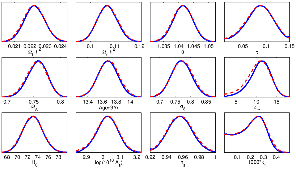
Introducing the infrared sharp cut on in the model we find sizably different gains
As before, the difference is due to the tighter bound on due to the inclusion of the SDSS data. In fact, the most likely values (ML) of and corresponding to are given in Table II.
| CDMsharpcut | (best fit) | (best fit) | (95% CL) |
|---|---|---|---|
| WMAP-3 only | 0.275 | 0.150 | |
| CMB+LSS | 0.268 | 0.051 |
The marginalized probabilities in the plane (converting to a flat prior on ) are shown in the two left panels of fig. 8. There are no significant changes on the other cosmological parameters.
This situation is also reproduced when the fastroll stage is included, that is when the fast roll transfer function eq. (58) and fig. 3 is used, treating the scale in eq. (59) as a MCMC parameter.
That is, in the MCMC analysis with fast-roll included, we use the initial power spectrum eq.(51) which is modified by the fast-roll transfer function . We computed once and forever from eq. (58) [see fig. 3]. is a function of and with the scaling form eq.(59), being an universal function.
We then find
Correspondingly, in Table III we report the most likely values (ML) of and (we report also the best fit for the quartic coupling for future use)
| CDMfastroll | (best fit) | (best fit) | (95% CL) | (best fit) |
|---|---|---|---|---|
| WMAP-3 only | 0.249 | 0.146 | 0.031 | |
| CMB+LSS | 0.266 | 0.058 | 1.322 |
where we used the marginalized probability in the plane as shown in the two right panels of fig. 8. Here denotes the model with the fast roll included.
We see a clear peak in when fast-roll or a sharp cut are introduced in the CMBSDSS fits.
We see that the gains in likelihood are more significant in the fast-roll case than in the sharpcut case. Clearly, this fit improvement through power modification by fastroll over power reduction by sharpcut is too small to constitue a real experimental evidence. But still, it is very interesting that the theoretically well founded approach based on fastroll works better than the purely phenomenological cutoff. This may be appreciated also from fig. 9 where the best fit for the multipoles are compared to the experimental data at low . We see that the oscillatory form of the fastroll transfer function , by depressing as well as enhancing the primordial power spectrum at long wavelengths, leads also to new superimposed oscillatory corrections on the multipoles. As far as fitting to current data is concerned, such corrections are more effective than the pure reduction caused by a sharp cutoff.
We did not display in figs. 9 and 10 the CDMsharpcut results since they are indistinguishable from the BNIsharpcut values.


We plot in fig. 10 the best fit for the multipoles compared to the experimental data at low . We see that for and fast-roll and sharpcut models yield rather similar results (and better than the CDM model) while for fast-roll produces a value closer to WMAP-3 data than sharpcut.
We plot in fig. 11 the multipoles computed in the best fit point to the WMAP-5 data compared to the experimental WMAP-5 data at low . We see that both fast-roll and sharpcut models produce a reduction of the low EE multipoles including the EE quadrupole.
Our fits imposing predict non-zero lower bounds on : at 95% CL, we find that when no cutoff is introduced, while when either the sharp cutoff or the fastroll are introduced. The best fit values of the other cosmological parameters remain practically unchanged as compared to CDM. Similarly their marginalized probability distributions are almost unchanged, with the natural exception of , which in BNI has a theoretical upper limit [see eq. (68)].


IV.3 Real Space Two Point TT-Correlator
We display in fig. 12 the real space two point TT-correlation function for CDM, sharpcut and fast-roll models,
We see that the CDM correlator becomes really different from the two others only for large angles . Since all -modes besides the lowest ones are practically identical in the three cases, this shows how dominant are the low multipoles in the large angle correlations. We also show the WMAP data, the width of the data is mostly due to the cosmic variance.
As is clear from fig. 12, both fast-roll and sharpcut models reproduce the two point correlator better than the pure slow-roll CDM model.

V The Total Number of e-folds of Inflation
Another interesting observation is possible concerning the number of efolds since horizon exit till the end of inflation. First of all let us clarify why in all our MCMC runs we keep fixed. The reason is that the main physics that determines the value of is not contained in the available data but involves the reheating era. Therefore, although technically possible, it is not reliable to fit solely with the CMB and LSS data within a pure, near scale-invariant slow roll scenario. On the other hand, the quadruple depression allows to set an absolute wavelength scale for the primordial power, so we can check the consistency of our assumptions about which fixes the total number of efolds of inflation.
In the case of the CDMfastroll model with the CMB+LSS datasets, the most likely value of the quartic coupling is slightly larger than unity. Then from fig. 4 we read a value for the ratio at horizon exit.
It is important to compare the quadrupole mode scale with the scale that characterizes the fast-roll stage.
The physical quadrupole () wavemodes today are related to the particle horizon today by
where the spherical Bessel function takes its maximun value, and is given by [6]
when one takes into account the acceleration of the universe expansion for . Therefore, using the present value [18] we obtain,
Notice that the value of is smaller than the characteristic scale .
We display in Table IV the relevant wavenumbers: and the number of efolds since the beginning of inflation when they exit the horizon. We see that the quadrupole modes exit the horizon during the fast-roll stage, approximately of an efold before the end of fast roll. The mode exit the horizon by , very close to the point where . That is, precisely exits the horizon when fast roll ends and becomes slow roll.
| at horizon exit | at horizon exit | |
|---|---|---|
| (WMAP) | ||
| (CosmoMC) |
.
We denote by in Table IV the pivot wavenumbers in the WMAP [8] and CosmoMC codes [13], where the indices and the running of are computed. Both ’s exit the horizon well inside the slow roll regime.
We read from Table IV that the total number of efolds of inflation is given by
since we have six efolds before the pivot wavenumber in CosmoMC exit the horizon followed by efolds of inflation.
We can compute the redshift since the begining of inflation till today comparing (today) with (at the begining of inflation). [Recall that ].
We use for the value obtained from the scale of inflation [15]
where is fixed by the amplitude of the scalar adiabatic fluctuations [8, 15]. We obtain
[Notice that these results are in agreement with the generic estimates eq.(4).] Therefore,
Assuming a sharp transition from inflation to radiation dominated expansion, the redshift can be written as
| (63) |
where is the scale factor at the begining of the radiation dominated era and is the total number of efolds during inflation (during fast-roll plus during slow-roll).
The scale factor at the beginning () and the end (, equilibration) of the radiation dominated era are related by
where and stand for the Hubble parameter at the beginning and at the end of the radiation dominated era, respectively. For simplicity we assume instantaneous reheating in these formulas.
Furthermore, and are related by [16]
where stands for the Hubble parameter today and for the matter fraction of the energy density of the universe today.
Using the current values of the cosmological parameters [18] we find
| (64) |
Inserting eq.(64) into eq.(63) yields
| (65) |
Since must be below its value at the beginning of inflation GeV [see eq.(5)], we conclude that
| (66) |
On the other hand, we know from BBN (Big Bang Nucleosynthesis) that is at least larger than 1 MeV. This together with eq.(65) yields the upper bound
| (67) |
Furthermore, our MCMC simulations give good fits for . The bound eq.(66) therefore favours which implies and GeV. In addition, from eqs.(66) and (67) we obtain the bounds .
In summary, the fast-roll stage explains the quadrupole suppression and fixes the total number of efolds of inflation [6, 7].
Our present MCMC analysis yields . More generally, the upper bound eq.(67) implies .
Changing from 50 to 60 does not affect significatively the MCMC fits we present in this paper. This is partially due to the fact that a change on can partially compensate a change on . Another hint to increase above 50 comes from WMAP-5 that gives a larger and using the theoretical upper limit for [14, 15]:
| (68) |
which gives for . This value is compatible with the value from WMAPBAOSN and no running [9].
Acknowledgements.
We thank L. Page, D. Boyanovsky, A. Hajian, R. Rebolo and D. Spergel for fruitful discussions. The MCMC simulations were performed on the Turing and Atena Linux Clusters of the Physics Department G. Occhialini of the University Milano-Bicocca.VI Appendix
As already shown in sec. IV, the four types of correlation multipoles, TT, TE, EE and BB, among the CMB anisotropies can be numerically computed with good accuracy within the CosmoMC program starting from a given cosmological model with a fixed value for all its parameters. To be precise, this computation is performed by the CAMB subprogram, which is an evolution of CMBFAST [17]. CAMB can also compute, with several levels of approximations, the matter power spectrum observable today given the primordial power spectrum of density perturbations.
On modern workstation CPU’s, the calculation of two thousand scalar multipoles (related to the primordial curvature fluctuations) and one thousand tensor multipoles (related to primordial gravitational waves) takes less than one second. Thus, within a given type of cosmological model, the theoretical predictions for different choices of parameters can be produced at a very high rate.
To test these predictions against the experimental data CosmoMC makes use of likelihood functions to assign different weights to different sets of correlation multipoles and matter power data. The experimental data and associated numerical code to evaluate such likelihoods is part of CosmoMC in the case of small–scale CMB experiments and LSS surveys. The data and likelihood routines for WMAP are not part of CosmoMC, but they can be downloaded from http://lambda.gsfc.nasa.gov/ and integrated quite easily into CosmoMC, since its interface to CMB likelihoods has been appositely designed for WMAP.
The WMAP likelihood code is particularly complex with respect to the other experiments, due to the wealth of experimental data, the variety of source of systematical errors and the importance of cosmic variance on lower multipoles. Indeed, it has significally changed and improved along the three WMAP releases. At any rate, it is used in CosmoMC exactly as released by the WMAP team.
Finally, CosmoMC provides the MCMC engine, that is, the routines to perform suitable random walks (the chains) in the parameter space of a give cosmological model in such a way to reconstructs the experimental probability for the parameters from the distribution of values produced along the chains. In our simulations we always employed the default Metropolis rule, where the one-step transition probability from one set of parameter values to the next is given by
where is a Gaussian proposal, or jump, probability and is the complete posterior likelihood, that is the product of the prior probability of choosing the starting point of the chain, times the likelihood obtained by comparing the theoretical prediction on multipoles (and matter power if LSS constraints are required) with the experimental data. As is well known from the theory of stationary Markov chains, in the limit of infinitely long chains no dependence is retained on and the reconstructed profile is that of only. Of course, since actual chains have a finite length, suitable convergence tests are needed to verify that such a reconstruction is accurate enough. On pc-cluster running several parallel chains at once, CosmoMC offers very effective tests of this kind.
In order to test our own models based on Binomial New Inflation, with or without sharp–cut or fast-roll, we needed to modify some routines in CosmoMC. Since our changes with respect to the CDM model are restricted to the primordial power spectrum, only routines relative to the so–called fast variables needed suitable modifications. Fast variables in CosmoMC are cosmological parameters that affect only the primordial spectrum so that, in a Monte Carlo step that proposes changes restricted to them, no need arises to perform the time–consuming recomputation of the transfer functions from a given primordial spectrum to observable multipoles. Slow variables such as the baryonic and dark matter fractions, , the optical depth , and the present Hubble parameter have the opposite definition. No change was done in the by far major portion of the CosmoMC program that deals with slow variables.
We recall also that we let only the four slow variables mentioned above vary in our MCMC run (to be precise, we used the default choice of CosmoMC which replaces with , the ratio of the approximate sound horizon to the angular diameter distance), keeping all other slow cosmological parameters, such as the parameter of the dark energy equation of state or the neutrino density fraction, to the values of the standard CDM model.
References
- [1] Kazanas D, Astrophys. J. 241: L59 (1980); Guth A H, Phys. Rev. D23, 347 (1981); Sato K, MNRAS, 195: 467 (1981).
- [2] See for example: Hu W and Dodelson S, Ann. Rev. Astron. Ap. 40: 171 (2002); Lidsey J, Liddle A, Kolb E, Copeland E, Barreiro T and Abney M, Rev. of Mod. Phys. 69: 373, (1997). Hu W, astro-ph/0402060. Mukhanov VF, Feldman HA and Brandenberger RH, Phys. Rep. 215:203 (1992). A. R. Liddle, D. H. Lyth, Cosmological Inflation and Large Scale Structure, Cambridge University Press, 2000; Phys. Rept. 231, 1 (1993) and references therein.
- [3] V. A. Belinsky, L. P. Grishchuk, Ya. B. Zeldovich, I. M. Khalatnikov, Phys. Lett. B 155, 232, (1985), JETP 62, 195 (1985).
- [4] G. F. Smoot et. al. (COBE collaboration), Astrophys. J. 396, 1 (1992).
- [5] D. Boyanovsky, H. J. de Vega, N. G. Sanchez, Phys. Rev. D 73, 023008 (2006).
- [6] D. Boyanovsky, H. J. de Vega, N. G. Sánchez, Phys. Rev. D 74, 123006 (2006).
- [7] D. Boyanovsky, H. J. de Vega, N. G. Sánchez, Phys. Rev. D 74, 123007 (2006).
- [8] D. N. Spergel et. al. (WMAP collaboration), astro-ph/0603449, Astrophys. J. Suppl., 170, 377 (2007).
- [9]
E. Komatsu et al. (WMAP collaboration), arXiv:0803.0547;
G. Hinshaw et al. (WMAP collaboration), arXiv:0803.0732;
M. R. Nolta et al.(WMAP collaboration), arXiv:0803.0593;
J. Dunkley et al. (WMAP collaboration), arXiv:0803.0586. M. R. Nolta et al.(WMAP collaboration), arXiv:0803.0593. - [10] A. de Oliveira-Costa, M. Tegmark, M. Zaldarriaga and A. J. Hamilton, Phys. Rev. D69, 063516 (2004); E. Gaztanaga et. al. Mon. Not. Roy. Astron. Soc. 346, 47 (2003). A. Hajian, astro-ph/0702723. O. Doré et al. Astrophys. J., 612, 81 (2004). A. Shafieloo, T. Souradeep, Phys.Rev. D70, 043523 (2004). A. de Oliveira-Costa and M. Tegmark, Phys.Rev. D74, 023005 (2006).
- [11] D. Schwarz, G. Starkman, D. Huterer and C. Copi, Phys. Rev. Lett. 93, 221301 (2004); C. Copi, D. Huterer, D. Schwarz and G. Starkman, Phys. Rev. D75, 023507 (2007); A. Rakic, D. Schwarz, Phys. Rev. D75, 103002 (2007);
- [12] N J Cornish, D N Spergel, G D Starkman, E Komatsu, Phys. Rev. Lett. 92, 201302 (2004); B F Roukema, B Lew, M Cechowska, A Marecki, S Bajtlik, Astronomy and Astrophysics 423, 821 (2004); J G Cresswell, A R Liddle, P Mukherjee, A Riazuelo ;Phys. Rev. D 73, 041302 (2006); M. Liguori, S Matarrese, M Musso, A Riotto, JCAP 408, 011 (2004); R. V. Buniy 2005; Int. J. Mod. Phys. A20,1095 (2005); R. V. Buniy, A. Berera, T. W. Kephart, Phys. Rev. D73, 063529 (2006); T. Multamaki, O. Elgaroy, Astronomy and Astrophysics 423, 811 (2004); C. Gordon, W. Hu, Phys.Rev. D70, 083003 (2004); T. R. Jaffe, A. J. Banday, H. K. Eriksen, K. M. Gorski, F. K. Hansen, Astrophys. J., 629, L1 (2005); C. Gordon, W. Hu, D. Huterer, T. Crawford, Phys.Rev. D72, 103002 (2005); C-H. Wu, K.-W. Ng, W. Lee, D.-S. Lee, Y.-Y. Charng, JCAP 0702, 006 (2007). L. Campanelli, P. Cea, L. Tedesco, Phys. Rev. Lett. 97, 131302 (2006), Phys. Rev. D76, 063007, (2007). Y. S. Piao, Phys. Rev. D71, 087301 (2005). M. Kawasaki, F. Takahashi, Phys. Lett. B570, 151 (2003). L. R. Abramo, L. Sodre Jr, C. A. Wuensche, Phys. Rev. D74, 083515 (2006). I-C. Wang, K-W. Ng, Phys. Rev. D 77, 083501 (2008); J. M. Cline, P. Crotty, J. Lesgourgues, JCAP 0309, 010, (2003).
- [13] A. Lewis, S. Bridle, Phys. Rev. D66, 103511 (2002). http://cosmologist.info/cosmomc/
- [14] H. J. de Vega, N. G. Sánchez, Phys. Rev. D74, 063519 (2006).
- [15] C. Destri, H. J. de Vega, N. G. Sánchez, Phys. Rev. D77, 043509 (2008).
- [16] Kolb EW and Turner MS, The Early Universe, Addison Wesley. Redwood City, C.A. 1990. M. Giovannini, astro-ph/0703730.
- [17] Seljak, U., M. Zaldarriaga, Astrophys. J. 469, 437 (1996).
- [18] W.-M. Yao et al., Journal of Physics G 33, 1 (2006).