http://www.dma.ens.fr/ levy/ \alttitleChamps d’holonomie markoviens bidimensionnels
Ce travail est consacré à la définition et à l’étude d’une classe de processus stochastiques indexés par des chemins tracés sur une surface, qui prennent leurs valeurs dans un groupe de Lie compact et qui satisfont une propriété d’indépendance conditionnelle analogue à la propriété de Markov. Nous appelons ces processus des champs d’holonomie markoviens bidimensionnels. L’exemple fondamental de cette sorte de processus est le processus canonique sous la mesure de Yang-Mills, qui a été construite d’abord par Ambar Sengupta [32] puis plus tard par l’auteur [21]. C’est aussi le seul champ d’holonomie markovien qui ait été construit avant ce travail. Le processus canonique sous la mesure de Yang-Mills est assez exactement aux champs d’holonomie markoviens ce que le mouvement brownien est aux processus de Lévy. Deux de nos principaux résultats affirment qu’à tout champ d’holonomie markovien suffisamment régulier est associé un processus de Lévy d’une certaine classe sur le groupe de Lie dans lequel il prend ses valeurs et réciproquement que pour tout processus de Lévy dans cette classe il existe un champ d’holonomie markovien auquel il est associé. Dans le cas particulier où le groupe de Lie considéré est un groupe fini, nous parvenons à réaliser ce champ d’holonomie markovien comme la monodromie d’un fibré principal ramifié aléatoire. Ceci nous rapproche de l’interprétation originelle de la mesure de Yang-Mills, issue de la théorie quantique des champs, comme mesure de probabilités sur l’espace des connexions sur un fibré principal.
Champ aléatoire, processus de Markov, processus de Lévy, groupe de Lie compact, graphe sur une surface, chemin rectifiable, revêtement ramifié, Yang-Mills, théorie de jauge sur réseau, limite continue
Two-dimensional Markovian holonomy fields
Abstract
We define a notion of Markov process indexed by curves drawn on a compact surface and taking its values in a compact Lie group. We call such a process a two-dimensional Markovian holonomy field. The prototype of this class of processes, and the only one to have been constructed before the present work, is the canonical process under the Yang-Mills measure, first defined by Ambar Sengupta [32] and later by the author [21]. The Yang-Mills measure sits in the class of Markovian holonomy fields very much like the Brownian motion in the class of Lévy processes. We prove that every regular Markovian holonomy field determines a Lévy process of a certain class on the Lie group in which it takes its values, and construct, for each Lévy process in this class, a Markovian holonomy field to which it is associated. When the Lie group is in fact a finite group, we give an alternative construction of this Markovian holonomy field as the monodromy of a random ramified principal bundle. This is in heuristic agreement with the physical origin of the Yang-Mills measure as the holonomy of a random connection on a principal bundle.
Key words and phrases:
Random field, Markov process, Lévy process, compact Lie group, graph on a surface, rectifiable path, ramified covering, Yang-Mills, lattice gauge theory, continuous limit1991 Mathematics Subject Classification
60G60, 60J99, 60G51, 60B15, 57M20, 57M12, 81T13, 81T27Introduction
The elementary theory of Markov processes establishes a correspondence between several types of objects among which transition semigroups and stochastic processes. These stochastic processes can take their values in fairly general spaces, but they are usually indexed by a subset of the real numbers, for the Markov property relies on the distinction between past and future. In the present work, we investigate a correspondence between certain transition semigroups and another kind of stochastic processes, where the notions of past and future are replaced by the notions of inside and outside. The processes that we consider are indexed by curves, or rather loops, drawn on a surface, and they take their values in a compact Lie group. We call them (two-dimensional) Markovian holonomy fields. They are Markovian in the following sense: if some piece of a surface is bounded by a finite collection of loops, then the values of the process on loops located inside this piece and outside this piece are independent, conditionally on the value of the process on the finite collection of loops which bounds this piece.
1. A -dimensional analogue
Let us start by discussing the -dimensional analogues of Markovian holonomy fields, which are just Markov processes looked at from a slightly unusual point of view. Let us choose a transition semigroup on some state space . For each , is a transition kernel on . Under suitable assumptions, we can associate to a homogeneous Markov process with values in , which we denote by . This Markov process is not really a single stochastic process, it is rather a collection of processes, essentially one for each initial condition at a specific time. In fact, if we consider restricted to segments, we can say that to each segment and each initial condition we associate a process with values in such that almost surely. Among the structure implied by the fact that is a subset of , what we really use is the topological structure of this interval, its orientation and our ability to measure the distance between any two of its points. Of course, in the present -dimensional setting, this structure suffices to characterize the interval up to translation, and the last sentence may seem pointless. Its content should however become clearer in the 2-dimensional setting. Let us push the abstraction a little further and try to define, for all compact -dimensional manifold , a process with values in . As we have just observed, we need an orientation of and a way to measure distances. Moreover, if is not connected, we want the restrictions of our process to the connected components of to be independent. So, let be an oriented compact connected Riemannian -dimensional manifold. There are not so many choices: is either homeomorphic to a segment or to a circle, it has a certain positive total length, and this information characterizes it completely up to orientation-preserving isometry. If is a segment of length , it is isometric to and there is no difficulty in defining the process given an initial condition. Before turning to the case of the circle, let us interpret the Markov property of in terms of these -dimensional manifolds.
Let and be two manifolds as above, isometric to segments. Let denote the manifold obtained by identifying the final point of with the initial point of . It is still homeomorphic to a segment. Choose an initial condition . We are able to construct two stochastic processes indexed by . Firstly, we can take as a segment on its own and simply consider the process with initial condition . But we can also proceed as follows. For all segment and all , let denote the distribution of the process with initial condition . Let us also denote by the disintegration of with respect to the value of at the final point of . Then the probability measure is the distribution of a process indexed by the disjoint union of and which takes the same value at the final point of and the initial point of . It can thus be identified with the distribution of a process indexed by . It is exactly the content of the Markov property of that the two measures that we have considered are equal:
| (1) |
This relation is an instance of the Kolmogorov-Chapman equation. This example illustrates in the simplest possible way the fact that the Markov property can be nicely formulated in terms of surgery of manifolds, in this case concatenation of intervals. Manifolds of dimension undergo another kind of surgery, when the two endpoints of a single interval are glued together (see Figure 1). If we try to mimic (1), we are tempted to define the distribution of a process indexed by the circle of length , seen as the interval of which the endpoints have been identified, by
| (2) |
which unfortunately is meaningless. Still, this formula is consistent with the fact that a circle has no boundary, so that there is no initial condition to specify. What we are pretending to define here is a bridge, a probability measure on closed trajectories in , from the transition semigroup .

Without aiming at the greatest possible generality, let us describe a situation in which this is possible. We assume that is a smooth finite-dimensional manifold, for example a vector space or a Lie group, which carries a Borel probability measure which is stationary for the semi-group . Finally, we assume that for all and all , the measure has a continuous density with respect to , which we denote by . In this situation, it is possible to define bridges of the Markov process between any two points of . Hence, for each segment , it is possible to define the finite measure which is the conditional distribution of given and , multiplied by the real number . With this definition, is not a probability measure in general but the relation holds. We can then define the process indexed by a circle of length by setting
| (3) |
The identification of a process indexed by circle with a process indexed by requires the choice of a base point on but the stationarity of implies that the resulting definition of is independent of this choice.
Let us summarize this discussion of the -dimensional case. Starting with a Markovian transition semigroup on with good properties, we have been able to associate to each compact oriented -dimensional Riemannian manifold, endowed with boundary conditions if it is homeomorphic to a segment, a stochastic process with values in indexed by the points of this manifold. This collection of processes exhibits a Markovian behaviour with respect to the operations of cutting or concatenation of manifolds.
2. The transition kernels of Markovian holonomy fields
A -dimensional Markovian holonomy field is a -dimensional analogue of the object just described. It is a collection of stochastic processes, one for each compact surface endowed with boundary conditions and some way of measuring areas. For each such surface, the process is indexed by a set of loops drawn on this surface. Moreover, these processes satisfy Markovian properties with respect to the operations of cutting surfaces along curves or gluing them along boundary components.
Before explaining this more carefully, let us discuss the important fact that loops can be concatenated when they have the same origin. We are interested in stochastic processes which satisfy a property of additivity with respect to the concatenation of loops. This requires that they take their values in a group and since this group will usually not be assumed to be Abelian, and denoted multiplicatively, we will rather call this a property of multiplicativity. Let us give a precise definition. If is a -dimensional manifold and is a point of , let be a set of loops on based at . We will discuss later which loops exactly we wish to consider. To each loop we can associate the inverse loop , which is simply traced backwards. Also, to each pair of loops we can associate their concatenation which we denote by . Let be a group, which plays the role of the space above. A stochastic process with values in is said to be multiplicative if
| (4) | ||||
| (5) |
We will also explain later why we chose to reverse the order on the right-hand side of this equality. For the moment, let us describe the transitions of a Markovian holonomy field.
Just as an interval has two extremities, a surface has a boundary which is topologically a disjoint union of circles. Let us consider a surface, with a certain number of boundary components. In contrast with the -dimensional case, even if the surface is oriented, its boundary components are indistinguishable from a topological point of view: any permutation of the boundary components can be realized by an orientation-preserving homeomorphism. So, let us arbitrarily declare that some of these components are incoming and the other are outgoing. Then we have a picture of our surface as realizing a cobordism, that is, a topological transition, between two sets of circles (see Figure 2). If the surface is oriented, then we orient incoming boundary components negatively and outcoming boundary components positively. This matters because, according to (4), the boundary conditions on the incoming components are associated with oriented loops: to each oriented incoming boundary component we associate an element of .

The comparison with the -dimensional case indicates that we are lacking a measure of time on our surface. The analogue of the ability to measure distances is the ability to measure areas. On a surface, this requires much less than a Riemannian metric, only a Borel measure with suitable regularity properties. We have now isolated the necessary structure: a Markovian holonomy field takes its values in a group which we denote by , and its transitions occur along surfaces with distinguished incoming and outgoing boundaries endowed with a measure of area. The associated transition kernels describe the distribution of the process on the outgoing circles conditionally on its values on the incoming ones.
There is a lot more variety of situations than in the -dimensional case, but fortunately for us, this variety has been very well understood for about a century and is easy to describe. Up to homeomorphism, a connected compact surface is characterized by the fact that it is orientable or not, by the number of connected components of its boundary, and by a single other topological invariant called its genus which can be any non-negative integer if the surface is orientable and any positive integer if it is not. Moreover, the only invariant of a smooth measure of area under diffeomorphisms is its total area. It turns out that, when one deals with orientable and non-orientable surfaces at the same time, the genus is not the most convenient way to label the possible topological types of surfaces. We prefer to work with what we call the reduced genus, which is simply the genus if the surface is not orientable, and twice the classical genus if it is orientable. The main advantage of the reduced genus is that it is additive with respect to the operation of connected sum.
Let us denote by the space of probability measures on . Then the transition kernel of a Markovian holonomy field can be listed as follows:
| (6) |
where the sign indicates the orientability of the surface, is its reduced genus, its total area and the number of its boundary components, of which are incoming and outgoing.
If , then the transition kernel is a measure on , if it is a function on and if , it is a real number. In order to avoid the problems that we have encountered with the circle in the -dimensional case, we will make fairly strong assumptions. Firstly, we will assume that is a compact Lie group. Such a group carries a unique probability measure invariant by translations, which we denote by . We will also assume that the transition kernels of the Markovian holonomy field that we consider can be put under the form
| (7) |
for some functions which are called the partition functions of the holonomy field. The exponents that we have introduced take care of the issue of orientation. They restore the symmetry between the boundary components of a surface, so that the partition functions are invariant by permutation of their arguments.
The possibility of gluing together boundary components of one or two surfaces leads to infinitely many variants of the Kolmogorov-Chapman equation which give as many relations between the partition functions. For instance, consider a cylinder of area with one incoming circle and one outgoing circle. A cylinder has genus (both classical and reduced) and the transition kernel associated to this surface is . By gluing the incoming circle of this cylinder along an outgoing circle of an arbitrary surface, we do not change this surface up to homeomorphism, we only increase its area by . Hence, we have the following relation between transition kernels:
| (8) | |||||
As another example, let us consider an orientable surface with at least one incoming and one outgoing circle. If we glue these circles one along the other in such a way that the result is still orientable, then we obtain a surface with two less boundary components, a classical genus increased by , hence a reduced genus increased by , and the same area. This example is reminiscent of the situation where we obtained a circle by identifying the two endpoints of a segment. It is thus not surprising that in this case, the Markov property is best expressed in terms of the partition functions, rather than the transition kernels. It reads
| (9) |
If we identify an outgoing circle with an incoming one in a non-orientable surface, then the reduced genus of the surface is also increased by . In this case, the Kolmogorov-Chapman equation is
| (10) |
A more unusual topological operation consists in identifying a boundary component of a surface with itself by an orientation-preserving involution (see Figure 4 page 4). Up to homeomorphism, this operation is equivalent to gluing a Möbius band along this boundary component. The resulting surface is always non-orientable and its reduced genus is increased by one. The corresponding relation for partition functions is
| (11) |
The equalities (8), (9), (10) and (11) essentially exhaust the types of relations that hold between the partition functions. Using these relations, we will prove that the whole set of partition functions of a Markovian holonomy field is determined by just those associated to a disk, a Möbius band and a three-holed sphere of arbitrary area. Indeed, any surface can be built from these three elementary bricks by a finite number of gluings. In fact, if the Markovian holonomy field is regular enough, then we will prove that all its transition kernels are determined by the sole transition kernels associated to disks. These transition kernels constitute a one-parameter family of probability measures on which turns out to form a continuous convolution semi-group, hence the collection of -dimensional marginals of a Lévy process on .
We are now able to give an idea of two of our main results. After giving an axiomatic definition of a -dimensional Markovian holonomy field with values in a compact Lie group (Definition 17.2), we will prove, under a suitable regularity assumption, that there is a classical Lévy process with values in associated with each Markovian holonomy field (Proposition 22.1). This Lévy process is characterized by the fact that its -dimensional distributions are the transition kernels of the holonomy field associated to disks. Moreover, all partition functions of the holonomy field can be expressed in terms of these -dimensional distributions (Proposition 21.10). Then, we will prove that for all Lévy process which satisfies some regularity properties, there exists a Markovian holonomy field to which this Lévy process is associated (Theorem 23.1). We do not settle in this work the question of the unicity of a Markovian holonomy field with a given associated Lévy process.
3. Markovian holonomy fields and the Yang-Mills measure
The Yang-Mills measure is to Markovian holonomy fields what the Brownian motion is to Lévy processes. It is indeed a Markovian holonomy field, whose associated Lévy process is the Brownian motion on . It is also the only Markovian holonomy field to have been constructed before the present work. The Yang-Mills measure has been the object of mathematical work since around 1990. It has been first constructed on an arbitrary compact surface by Ambar Sengupta [32]. The author has later given a different construction of essentially the same measure in [21]. One of the by-products of the present work is to provide another construction of the Yang-Mills measure, which really is very close to that given in [21]. Yet, we would like to emphasize several aspects in which it differs from the previous ones.
The first difference is a slight shift of point of view which we have already illustrated. Instead of considering a surface, choosing boundary conditions and constructing a process indexed by some class of loops on this specific surface, we now consider as one single object a whole collection of processes indexed by loops on all possible surfaces. The advantage of this view is that is leads quite naturally to an axiomatic characterization of Markovian holonomy fields. The one that we propose is inspired by the classical definition of a Markov process and by the axiomatic definition of a topological quantum field theory.
Another difference lies in the class of loops that we consider on a surface. Indeed, on a surface endowed with boundary conditions, a measure of the area, and a base point , the Yang-Mills measure produces a -valued stochastic process for some class of loops , of which we had promised a discussion earlier. In the two previous constructions of the Yang-Mills measure mentioned above, the loops to which one was able to attach a random variable were finite concatenations of very special curves, for example segments of submanifolds in the author’s construction. On the other hand, it was proved in [21] that the mapping is continuous in norm on the class of loops considered there endowed with the topology of uniform convergence and convergence of the length. This suggested that it should be possible to associate a random variable at least to each loop of finite length. This is indeed what we achieve in the present construction, thus giving more coherence between the regularity property of the stochastic process and the set of loops on which it is defined. Let us point out that it is not necessary to be able to measure lengths in order to decide if a loop has finite length. Indeed, a diffeomorphism does not alter the fact that a curve has finite or infinite length. Thus, the definition of as the set of loops on with finite length based at does not require the choice of a Riemannian metric on , a smooth structure is more than enough. It is natural to wonder if one could define the Yang-Mills measure or any other Markovian holonomy field for a significantly larger class of loops. We believe that this is not possible with only the techniques used in this work, and probably very difficult anyway. We shall discuss this in relation with the Brownian motion indexed by loops defined below.
The third important difference between this work and the existing constructions of the Yang-Mills measure concerns the group in which the stochastic process takes its values, which we have already denoted by . Since the Yang-Mills measure is associated with the Brownian motion on , it was natural to assume that it was a connected group. In the present work, the Brownian motion is replaced by a Lévy process, thus a process with jumps. This opens the possibility of considering non-connected compact Lie groups and in particular finite groups. In the case of finite groups, the Lévy processes have a very simple structure and we are able to give a completely geometrical picture of Markovian holonomy fields, at least the ones that we are able to construct. We will discuss this in more detail later after recalling briefly the physical and geometrical motivation for the study of Markovian holonomy fields.
4. The real Brownian motion indexed by loops
In this paragraph, we present an example of a stochastic process which does not exactly fit into our definition of Markovian holonomy fields, but is in a sense simpler and should absolutely be kept in mind as a fundamental example. We will also take this example as an opportunity to finish our introductory discussion of the role of loops with finite length.
Consider the plane endowed with the Lebesgue measure denoted by . Let be a white noise, that is, an isometry into a Hilbert space of centred real Gaussian random variables. Let be a continuous loop. For each point , the topological index of with respect to is an integer denoted by and defined, if we identify with , by
| (12) |
where is any piecewise smooth loop which is uniformly close enough to , for example closer than the distance of to the range of . Let us say that the loop winds mildly if its range is negligible and . In this case, it is legitimate to define
| (13) |
Definition 4.1.
The stochastic process is called the Brownian motion indexed by loops on .
To each subset of the plane, we may associate a -field which we define by
| (14) |
If is a Jordan curve in , then we denote respectively by and the bounded and unbounded connected components of , which we call the interior and exterior of . A basic property of the white noise is that it associates independent random variables to functions with disjoint supports. This implies the following property of the Brownian motion indexed by loops.
Proposition 4.2.
Let and be two Jordan curves with disjoint interiors. Then the -fields and are independent.
Proof.
If is a loop whose range is contained in , then the support of is also contained in . The same holds for and the result follows. ∎
Let us now prove a Markov property.
Proposition 4.3.
Let be a Jordan curve with negligible range. The -fields and are independent conditionally on .
Proof.
By the Jordan curve theorem, a Jordan curve with negligible range winds mildly. Let be the line in generated by . Let (resp. ) be the closed linear subspace of generated by for which winds mildly and (resp. ). The inclusions are straightforward. They are actually equalities but we do not need this fact. In particular, . Moreover, with the notation for the orthogonal complement, we have
In particular, the orthogonality relation holds and the result follows. ∎
It is illuminating to discuss the role of loops of finite length with the example of the Brownian motion indexed by loops in mind. A loop with finite length admits a Lipschitz continuous parametrization. Hence, its range has Hausdorff dimension , unless it is constant. In any case, its range is negligible. The fact that its topological index is square-integrable is not at all obvious. It is granted by a generalization of the isoperimetric inequality discovered by T. Banchoff and W. Pohl. We denote the length of by .
Theorem 4.4 (Banchoff-Pohl).
Let be a Lipschitz continuous loop. Then
The original reference for this theorem is the article of T. Banchoff and W. Pohl [5]. They prove the inequality for a loop of class . An elementary proof of the inequality for rectifiable curves can be found in a paper by A. Vogt [34].
Of course, there are many loops with infinite length whose topological index is square-integrable, for instance fractal Jordan curves or simply loops of infinite length whose range is contained in a line. It would probably be difficult to characterize the set of loops which wind mildly in a way which differs significantly from its definition. Nevertheless, on the scale of roughness given by the -variation, as defined by L.C. Young [39], the space of rectifiable loops is the largest which contains only loops which wind mildly. Recall that the -variation of a loop is defined as the supremum over all subdivisions of of the quantity . A loop has finite length if and only if it has finite -variation. A loop with finite -variation for has negligible range.
Proposition 4.5.
There exists a loop such that has finite -variation for all and .

Proof.
For each , let be the loop based at the origin which goes once along the circle of radius through the origin, tangent to the horizontal axis and contained in the upper half-plane. Assume that is parametrized at constant speed by an interval of length . Let be the uniform limit of the finite concatenations as tends to infinity. This limit exists because the radii of the circles tend to as tends to infinity. For all , the -variation of raised to the power is equal, up to some constant, to , hence it is finite. On the other hand, the squared norm of is . ∎
5. Markovian holonomy fields and gauge fields
The original motivation for the study of processes indexed by loops is issued from theoretical physics, indeed from quantum field theory and more precisely from quantum gauge theories. Let us explain this with the example of electrodynamics. The classical theory of electrodynamics, as established in the second half of the nineteenth century, is summarized by the Lorentz law and Maxwell’s equations. Maxwell’s equations relate the electric and the magnetic field to the density of electric charge and the density of electric current in space. In order to derive these equations from a principle of least action, which is usually the first step in the procedure of quantization of a physical theory, it is convenient to express the electric and magnetic fields in terms of a scalar potential and a vector potential. These potentials are not uniquely defined by the fields and this indeterminacy is called the gauge symmetry of the theory. It turns out that the geometric nature of the pair formed by the scalar and vector potentials is that of a connection on a principal bundle with structure group over the space-time. At the level of rigour of this discussion, we do not make a serious mistake by identifying this object with a differential -form on the space-time. This -form is usually denoted by and called the gauge field. The exterior differential of the gauge field is a mixture of the electric and magnetic fields called the electromagnetic field and denoted by . The relation implies the equality , which is equivalent to the two homogeneous Maxwell equations. The two inhomogeneous equations can be put under the form , where is the Hodge operator on space-time associated with the Minkowski metric, and is a differential -form built from the densities of charge and current.
Most importantly for us, the gauge field, the object in terms of which the classical electrodynamics is best described, is a differential -form on space-time. The most natural way to evaluate a -form is to integrate it along paths. In the case of electrodynamics, the gauge symmetry of the theory implies that any two gauge fields which differ by a total differential describe the same physics. This indicates that the natural gauge-invariant functionals of the gauge field are in fact its integrals along loops.
If instead of doing quantum mechanics we prefer to do statistical mechanics, then we turn the Minkowski space-time into a Euclidean space-time and put on the space of gauge fields the Gibbs measure corresponding to the action which gives back Maxwell’s equations through the least action principle. In an empty space-time, this action is called the Yang-Mills action and it is essentially the squared norm of the electromagnetic field. The natural way to study random gauge fields is to do so through their integrals along loops, and this constitutes indeed a stochastic process indexed by loops. The Markov property of such a process, in this physical context, reflects the following property of locality of the Yang-Mills action: if the space-time is partitioned into several regions, then each region contributes to the action by a quantity which can be computed from the values of the field inside this region only.
In general, the random object that we are studying is thus an analogue of the electromagnetic field, or rather of the gauge field formed by the scalar potential of the electric field and the vector potential of the magnetic field. Let us give an idea of the physical meaning of the gauge field . This field interacts with particles which carry an analogue of electric charge. In fact, the -form takes its values in the Lie algebra of a Lie group and the charge of a particle is mathematically a linear action of on some vector space in which the wave function of the particle takes its values. For example, in the case of electrodynamics, the group is , the wave functions take their values in and for a particle of charge , where is the charge of the electron, the group acts on be the representation . The exponential of the integral of the gauge field along a certain loop, as an element of , describes the modification of the phase of the wave function of a particle which travels along . More generally, let be a loop. Assume that is a Lie group and that is a differential -form on with values in the Lie algebra of . Then, under fairly weak regularity assumptions, the differential equation
| (15) |
has a unique solution . The element determined by (15) is called the holonomy of along and this is why we call our processes holonomy fields. The action of this element of on the left on the vector space in which the wave function of a particle takes its values determines how the state of a particle is modified when it travels along . The reversed order in the right-hand side of (5) is due to the fact that the state of a particle travelling along the concatenation of and is modified first by the transformation due to the displacement along and then by the transformation due to the displacement along .
6. Finite groups, gauge fields and ramified coverings
When the group is finite, the interpretation that a Markovian holonomy field is a reflection of a probability measure on a space of connections or differential -forms with values in the Lie algebra of becomes awkward. Indeed, this Lie algebra is the null vector space. Topologically, a principal bundle with finite structure group is a covering and it carries a unique connection, which is flat. If is simply connected, the holonomy along any loop is the unit element of . On the other hand, there exist Markovian holonomy fields with values in finite groups, which are non-trivial processes indexed by loops, even on the sphere .
When is finite, the correct geometric picture is the following: a Markovian holonomy field with values in is the monodromy of a random ramified -bundle. By a ramified -bundle, we mean a ramified covering whose regular fibres are endowed with a free transitive action of , or equivalently, a principal -bundle over the complement of a finite set. There is still a unique connection on a ramified principal bundle and this connection is flat at each point which is not a ramification point, but each ramification point acts like a macroscopic amount of curvature concentrated at a single point. For instance, if is an integer, then the mapping from to itself is naturally a ramified -bundle. The group acts by multiplication on , freely and transitively on the fibres of the covering map . Any loop which goes once positively around a disk which contains has monodromy , no matter how small this disk. This is consistent with the picture of a concentration of curvature at .
The idea that the Yang-Mills measure, or a Markovian holonomy field, with values in a connected Lie group is a probability measure on a space of connections looked at through its holonomy is only a guide for the intuition and has no firm rigorous ground. On the contrary, the fact that a large class of Markovian holonomy fields with values in a finite group can be realized as the monodromy of a random ramified -bundle is a theorem that we will prove. In the intuitive picture of the Yang-Mills measure, the curvature of the random connection is supposed to have the distribution of a white noise. The correct distribution of the ramified -bundles which correspond with a given Markovian holonomy field can be roughly described as follows: first choose the ramification locus by throwing a Poisson point process on the surface with intensity the measure of area, then give a weight to every ramified -bundle with this ramification locus which depends on its monodromy at each ramification point and the Lévy process associated to the Markovian holonomy field.
7. Organization
The present work consists of five chapters. In Chapters 1 and 2, we develop the tools and prove most of the technical results that we use in our study of Markovian holonomy fields. The first chapter covers the topology of surfaces and their surgery, the topological space of paths on a surface, the fundamental notion of graph on a surface, which we treat both topologically and combinatorially, and finishes with a discussion of Riemannian metrics. The second chapter introduces the space of multiplicative functions of paths with its measurable structures and its uniform measure. The last section is devoted to a study of the free group of loops in a graph in relation with this uniform measure.
In Chapter 3, we define Markovian holonomy fields and their discrete analogues. We prove the first central result of this work (Theorem 18.9) which encapsulates in an abstract way and extends the procedure which allowed us, in our previous construction of the Yang-Mills measure, to take the continuous limit of a discrete gauge theory. In our present language, we prove that every regular discrete Markovian holonomy field can be extended in a unique way to a regular Markovian holonomy field.
In Chapter 4, we prove that a regular Markovian holonomy field with values in a compact Lie group determines a classical Lévy process in , which in turn determines completely the partition functions of the holonomy field (Propositions 22.1 and 21.10). We then prove that each Lévy process of a wide class can be obtained in this way (Theorem 23.1). Whether or not two distinct Markovian holonomy fields can have the same associated Lévy process is a natural question which we do not settle here.
In Chapter 5, we prove that when the group is finite, the Markovian holonomy field constructed in the previous chapter is the monodromy process of a random ramified covering (Theorem 27.2). In fact, most of the chapter is devoted to the construction of this random ramified covering.
The choice that we have made of concentrating to the extent possible the technical results in the first two chapters has the obvious drawback that the results exposed there often lack their real motivation, and that a linear reading of these two chapters may not be very rewarding. We hope that this is compensated by the fact that the study of Markovian holonomy fields themselves is much more straightforward than it would be if one had to constantly interrupt the exposition to prove technical results. In order to allow as much as possible the possibility of jumping from a section to another, we have included an index of notation which should be helpful in locating the first occurrence of a notation or a symbol.
8. Bibliography
The original paper of C.N. Yang and R. L. Mills where they introduced non-Abelian gauge theories appeared in 1954 [38]. An explicit description of the Yang-Mills measure on a lattice was given by A. Migdal in 1975 [28]. The importance of the -dimensional Yang-Mills theory in relation with the geometry of the moduli space of flat connections was emphasized by E. Witten in two papers published in the early 1990’s [36, 37].
An introduction to some aspects of the physics of gauge theories accessible to a mathematician can be found in the book by J. Baez and J. Muniain [4]. The book by D. Bleecker [6] is a mathematical exposition of the theory of connections on a principal bundle with a strong bias towards gauge theories. The mathematical reference on connections is the book by S. Kobayashi and K. Nomizu [19].
The mathematical study of the Yang-Mills measure was developed around 1985 by S. Albeverio, R. Høegh-Krohn and H. Holden [1, 2], L. Gross [15, 16], C. King and A. Sengupta [17], B. Driver [9, 10]. The idea that one could construct a variant of the Yang-Mills measure associated to a Lévy process which is not necessarily the Brownian motion was already present, twenty years ago, in the work of Albeverio et al. [2]. A. Sengupta gave the first construction of the measure on the sphere in 1992 [31] and on an arbitrary compact surface in 1996 [32]. The author gave another construction on an arbitrary surface in 2003 [21], later refined to take non-trivial principal bundles into account [22]. In a different direction, around 1990, D. Fine has investigated the Yang-Mills measure in [11, 12] with a focus on the geometrical structure of the space of connections on a principal bundle.
The fact that gauge theories with finite structure groups are related to random ramified coverings had already been observed by A. D’Adda and P. Provero [7]. Ramified coverings are also important in relation with the large limit of the 2-dimensional Yang-Mills theory, for a reason which is not directly related to the content of the present work. This relation has been revealed by D. Gross, in collaboration with W. Taylor [14] and A. Matytsin [13]. It has recently been investigated by the author [23].
Chapter 1 Surfaces and graphs
In this chapter, we introduce the tools of topology and geometry of surfaces that we use in the rest of this work. We set up the notation, collect the necessary classical results and prove less classical ones. After a short review of compact surfaces, we describe their surgery and study in some detail the paths and graphs drawn on them. In particular, we describe carefully the boundary of a face of a graph. Then we define the group of reduced loops based at a point in a graph and recall why it is free. In the next chapter, we will prove the existence of sets of generators of this group with specific properties. Finally, we discuss Riemannian metrics on surfaces in relation with our problem.
9. Surfaces
9.1. Classification of surfaces
Let us start by recalling the definition of a surface.
Definition 9.1.
A topological compact surface is a Hausdorff compact topological space in which every point admits a neighbourhood homeomorphic to or to .
A smooth compact surface, or simply a compact surface, is a topological compact surface equipped with a structure of smooth 2-dimensional manifold with boundary.
The distinction between topological and smooth surfaces is not essential, as the following result shows.
Theorem 9.2.
Any topological compact surface is homeomorphic to a smooth compact surface. Moreover, two smooth compact surfaces are diffeomorphic if and only if they are homeomorphic.
The classification theorem for compact surfaces is thus the same for smooth and topological surfaces, and we describe it now. We warn the reader that we are using a slightly unorthodox convention about the genus of a surface.
Let us describe two infinite series of surfaces. The first series is built from the torus, which is the Cartesian product of two circles. For each even integer and each integer , let be the surface obtained by removing pairwise disjoint open disks from the connected sum of tori. For , the surface is a sphere with holes. The second series is built from the projective plane, which is the quotient of the unit sphere of by the group of isometries . For each integer and each , let be the surface obtained by removing pairwise disjoint open disks from the connected sum of projective planes.
Recall that a smooth compact surface is orientable if it carries a non-vanishing differential 2-form. We say that a topological compact surface is orientable if a smooth compact surface to which it is homeomorphic is orientable.
Theorem 9.3.
Any connected orientable topological compact surface is homeomorphic to one and exactly one of the surfaces . Any connected non-orientable compact surface is homeomorphic to one and exactly one of the surfaces . Any oriented smooth compact surface admits an orientation-reversing diffeomorphism.
We call the integer which appears in this classification the genus of a surface. For orientable surfaces, it is twice the number which is usually called the genus. The advantage of our convention is illustrated by Proposition 9.4. We denote the genus of a surface by and the number of connected components of its boundary by
With this notation, we have and . Let us define a binary operation on by setting and . If and are two compact topological surfaces, we denote by the connected sum of and which is the surface obtained by removing a small disk from and and gluing the two resulting surfaces along the boundaries of these disks. Of course, this surface is defined up to homeomorphism only.
Proposition 9.4.
Let and be two surfaces of the list described above. Then
| (16) |
Proof.
It is clear that has boundary components. Moreover, the connected sum of two manifolds of the same dimension is orientable if and only if both manifolds are. The only non-trivial point is that the value of the reduced genus is correct when exactly one of the two surfaces and is orientable. In this case, since the operation of connected sum is commutative and associative, this boils down to the fact that the connected sum of a projective plane and a torus is homeomorphic to the connected sum of three projective planes. This is a classical result, proved as Lemma 7.1 in [27]. ∎
It is useful to keep in mind that if is a non-orientable compact topological surface, then the connected sum of with the torus is homeomorphic to the connected sum of with the Klein bottle .
The fundamental groups of surfaces are most easily described by generators and relations. We denote by the group generated by subject to the relations .
Theorem 9.5.
The fundamental groups of compact surfaces are, up to isomorphism, the following.
1. and for all ,
2. For all and all , is free of rank .
3. For all , .
4. For all and all , is free of rank .
It follows from this theorem that a compact surface is not characterized up to homeomorphism by its fundamental group. For example, a sphere with three holes and a torus with one hole both have a fundamental group which is free of rank 3. However, closed surfaces, that is, surfaces without boundary, are indeed characterized by their fundamental group.
If is a closed compact surface, then the reduced genus of is the minimal number of generators in a presentation of the fundamental group of . On the other hand, if has a non-empty boundary, then its fundamental group is free of rank .
The boundary of a compact surface is a finite union of circles. If a surface is oriented, then every connected component of carries an induced orientation, such that the surface stays on the left of a person walking along the boundary in the positive direction.
Definition 9.6.
Let be a compact surface. We denote by the set of connected components of the boundary of , each taken twice, once with each orientation. If is oriented, we denote by the subset of formed by the oriented connected components of which bound positively.
Any diffeomorphism of a compact surface induces a diffeomorphism of its boundary. We need to know which diffeomorphisms of the boundary can be obtained in this way. For this, observe that if the boundary of an oriented surface has connected components, then, among the distinct orientations of , the distinct orientations of determine preferred orientations. We say that a diffeomorphism of is orientation-preserving if it preserves these orientations and orientation-reversing if it exchanges them. Of course, if , then there exist diffeomorphisms of which are neither orientation-preserving nor orientation-reversing.
Theorem 9.7.
Let be a smooth compact surface. If is non-orientable, then any diffeomorphism of can be extended to a diffeomorphism of . If is orientable, then any orientation-preserving (resp. orientation-reversing) diffeomorphism of can be extended to an orientation-preserving (resp. orientation-reversing) diffeomorphism of .
9.2. Surgery of surfaces
Surfaces undergo natural operations of surgery such as cutting along a curve or gluing one or two boundary components. When one performs gluings and wants to keep track of where they have occurred, one ends up with surfaces which carry marks. On the other hand, when one cuts a surface along one or several curves, a convenient way of keeping track of what has been done is to maintain an involution of the set of boundary components of the current surface.
Definition 9.8.
A marked surface is a pair , where is a smooth compact surface and is a finite collection of pairwise disjoint oriented smooth -dimensional submanifolds of the interior of , such that an oriented curve belongs to if and only if the same curve with the opposite orientation belongs to . The elements of are called marks.
The marked surface is said to be oriented if every connected component of is orientable and oriented.
Let us emphasize that on a marked surface, even an oriented one, the marks do not carry a preferred orientation. The group acts on by reversing the orientation, and we denote this action by .
Definition 9.9.
A tubular pattern is a triple where is a marked surface and is an involution of which commutes to the orientation reversal, that is, which satisfies . If , the tubular pattern is said to be split.
Let be a tubular pattern. Choose . If is a component of distinct from , then is meant to be identified with by an orientation-preserving diffeomorphism. If , then is not meant to be glued or altered in any way. Finally, if , then is meant to be glued on itself according to an orientation-preserving involution. Of course, this way of encoding the possible gluing operations is purely conventional.
We define now the basic operation of surgery, which is the operation of gluing.
Definition 9.10.
Let and be two tubular patterns. A smooth mapping is called an elementary gluing if one of the following sets of conditions is satisfied.
1. The mapping is the quotient map which identifies with by an orientation-preserving diffeomorphism for some such that . Moreover, and, on , . Such a gluing is called binary, and the pair of curves is called its joint.
2. The mapping is the quotient map which identifies the points of by pairs according to an orientation-preserving smooth involution for some such that . Moreover, and, on , . In this case, the gluing is called unary and the pair of curves is called its joint.
A gluing is a map which can be written as the composition of several elementary gluings. A gluing is complete if the involution of the set of boundary components of the target surface is the identity.
Up to homeomorphism of the underlying surfaces and disregarding the markings, performing a unary gluing along a boundary component is equivalent to gluing a Möbius band along this boundary component. The result of this operation is never orientable.

The other basic surgery operation is that of splitting. It is really the same thing as a gluing, looked at in the other direction.
Proposition 9.11.
Let be a tubular pattern with . Choose . Then there exists a tubular pattern , and an elementary gluing such that the joint of is . Moreover, this gluing is unique up to isomorphism: if and satisfy the same properties, then there exists a diffeomorphism such that , and .
This result is intuitively obvious and yet it lacks concise rigorous proof. Considering that E. Moise, in the reference book [30], defines the splitting operation by a picture (Figure 21.1), we feel excused for not trying what would be a lengthy and uninstructive proof. Instead, let us make some comments on this result.
The surface can be defined as the topological space underlying the universal completion of the metric space , where is the restriction to of an arbitrary Riemannian distance on . The universal property of the completion actually provides us with a continuous gluing map.
It is easy to determine from the pair if the gluing is binary or unary. In fact, the gluing is unary if and only if does not admit an orientable neighbourhood, which is equivalent to the fact that for every neighbourhood of there exists a neighbourhood such that is connected. Another equivalent statement is that admits a compact neighbourhood which is homeomorphic to a Möbius band of which is an equator.
When these equivalent properties do not hold and the gluing is binary, there is an issue of orientation about the way in which the two boundary components of which are glued together are identified. If is orientable, then is also orientable, because a gluing performed on a non-orientable surfaces always results in another non-orientable surface, and the identification must be orientation-reversing. If is non-orientable, then two situations arise. Either is orientable, in which case the identification must be orientation-preserving, or is non-orientable. In this last case, any identification of the two boundary components is convenient. This is not in contradiction with the uniqueness part of the statement, since thanks to Theorem 9.7, any diffeomorphism of the boundary of a non-orientable compact surface can be extended to the whole surface.
Let be a marked surface. By successively applying Proposition 9.11 to the marks of , one eventually gets a tubular pattern with no marks, from which one can reconstruct .
Proposition 9.12.
Let be a marked surface. Let be the associated tubular pattern. There exists a tubular pattern and a smooth mapping which is a complete gluing in the sense of Definition 9.10. This gluing is unique up to isomorphism. The pattern is called a split tubular pattern of .
Definition 9.13.
Let be a marked surface. Let be a split tubular pattern of . Assume that is connected. We define the split reduced genus of as the reduced genus of . We denote it by .
10. Curves and paths
10.1. Definitions
In the theory of Markovian holonomy fields, curves and paths on a surface play the role of points of a time interval for classical Markov processes. We warn the reader that the words curve and path are not interchangeable in this work: a path is a curve with finite length.
Definition 10.1.
Let be a topological compact surface. A parametrized curve on is a continuous curve which is either constant on or constant on no open sub-interval of . The set of parametrized curves is denoted by .
Two parametrized curves on are said to be equivalent if they differ by an increasing homeomorphism of . An equivalence class is simply called a curve and the set of curves on is denoted by .
A continuous loop is a curve whose endpoints coincide. A continuous loop is said to be simple if it is injective on .
If is a curve, then we denote respectively by and the starting and finishing point of . We denote its inverse by . It is defined as the class of the parametrized curve , which does not depend on the particular parametrization of . The concatenation of curves is defined in the usual way. It is only partially defined on but associative whenever this makes sense.
The space is too large for many of our purposes. Let us define another space of curves which we call paths. Let be a smooth compact surface endowed with a Riemannian metric. Let be a Lipschitz continuous curve. Then the derivative of is defined almost-everywhere and its norm is bounded above. We are going to consider curves whose speed is also bounded below by a positive constant. Since the range of a curve is compact, this notion would be independent of the choice of the Riemannian metric on any smooth manifold.
Definition 10.2.
Let be a smooth compact surface. A parametrized path on is a continuous curve which is either constant or Lipschitz continuous with speed bounded below by a positive constant. The set of parametrized paths is denoted by .
Two parametrized paths on are said to be equivalent if they differ by an increasing bi-Lipschitz homeomorphism of . An equivalence class is simply called a path and the set of paths on is denoted by .
A loop is a path whose endpoints coincide. The set of loops is denoted by . A loop is said to be simple if it is injective on .
We use for paths the same notation as for curves. If is a path, we denote its endpoints by and , and its inverse by . The concatenation of paths is also associative whenever it is defined. When is endowed with a specific Riemannian metric, we usually identify with the subset of consisting of paths which are parametrized at constant speed.
While the inclusion does not determine an inclusion , because we are not using the same equivalence relation on parametrized curves and parametrized paths, it is true that a path, as a set of parametrized curves, is a subset of a unique curve. Moreover, two parametrized paths which are equivalent as parametrized curves are also equivalent as parametrized paths. Hence, there is a natural injection which we use without further comment.
Let us define a relation on by saying that two loops are related if and only if there exists such that and . It is not difficult to check that this is an equivalence relation.
Definition 10.3.
Let be a smooth compact surface. A cycle is an equivalence class of loops for the relation on just defined. We call non-oriented cycle a pair where is a cycle. We say that a cycle is simple if one of its representatives (hence all) are simple loops.
A cycle is simply a loop from which one has forgotten the origin. It is important to observe that an oriented -dimensional submanifold of determines a simple cycle. Another definition derived from that of loops and that will be useful is the following.
Definition 10.4.
A path is called a lasso if there exists a path and a simple loop such that .
Lemma 10.5.
Let be a lasso. There exist a unique path and a unique simple loop such that . The path is called the spoke of and the simple loop the meander of .
Proof.
Endow with a Riemannian metric. Assume that is parametrized at constant speed by . Then the meander of is the restriction of to the largest interval of the form on which is injective. ∎
We will use the topology of uniform convergence on .
Definition 10.6.
Let be a compact surface endowed with a Riemannian metric, whose Riemannian distance we denote by . Let be two curves of . We define
where the infimum is taken over all parametrizations of and .
The distance depends on the Riemannian metric chosen on . However, the topology on does not.
Lemma 10.7.
Let be a compact surface. The distances on associated with any two Riemannian metrics on are equivalent.
Proof.
Since is compact, the Riemannian distances on determined by any two Riemannian metrics are equivalent. ∎
On , we will use a topology which is stronger than the trace of the uniform topology. We use an analogue of the topology of convergence in -variation of Lipschitz continuous paths, for which a sequence of Lipschitz continuous paths in a Euclidean space converges if it converges uniformly and the sequence of the derivatives of the paths converges in . For the moment, we introduce a metric on which depends on a Riemannian metric on and is apparently weaker than the distance in -variation.
When is a path on a Riemannian surface, we denote by its length.
Definition 10.8.
Let be a compact surface endowed with a Riemannian metric. Let be two paths on . We define
It is not obvious, and we will prove in the next section, that the topology induced by on does not depend on the Riemannian metric on . Moreover, we will prove that this topology can be metrized by a distance for which is a complete metric space.
The topology on induced by the distance is the only one that we consider in this work and it is always the one to which we refer when we say that a sequence of paths converges. We will often add a condition on the endpoints of the paths which we consider.
Definition 10.9.
Let be a sequence of paths on . Let be a path on
. We say that converges to with fixed endpoints if
1. as ,
2. for all , and .
When is endowed with a Riemannian metric, we will also make use of piecewise geodesic paths.
Definition 10.10.
Let be a compact surface endowed with a Riemannian metric . We define as the subset of containing the piecewise geodesic paths, that is, the finite concatenations of segments of geodesics.
The letter stands for affine, instead of the letter which will be used for a lot of other things. We claim that is dense in . Indeed, there is an obvious way to approximate an arbitrary path by piecewise geodesic ones. This definition will be useful at a later time.
Definition 10.11.
Let be a compact surface endowed with a Riemannian metric . Consider , identified with a path parametrized at constant speed. Let be an integer. Assume that is smaller than the injectivity radius of . For each , let be the minimizing geodesic which joins to . Then define by
Proposition 10.12.
Let be a compact surface endowed with a Riemannian metric . For all path , the sequence defined for large enough converges to with fixed endpoints. In particular, the space is dense in for the convergence with fixed endpoints.
Proof.
Let be large enough for the path to be defined. It has the same endpoints as by construction. Let us parametrize it in such a way that for each , the restriction of to is the minimizing geodesic which joins to . It is straightforward that
Hence, converges uniformly towards . Since the length is lower semi-continuous with respect to pointwise convergence, this implies that . On the other hand, , hence converges to . ∎
10.2. The complete metric space of rectifiable paths
The goal of this section is to prove that the topology that we have introduced on does not depend on a particular choice of a Riemannian metric on and can be metrized by a complete distance. Let us start by a negative result.
Lemma 10.13.
Let be a compact surface endowed with a Riemannian metric. The metric space is not complete.
Proof.
Let be a segment of minimizing geodesic parametrized at constant speed. For each , define by . For all , . Moreover, for all , . Hence, the sequence is a Cauchy sequence for which converges uniformly to . Its only possible limit is , but does not converge to .∎
The main result of this section is the following.
Proposition 10.14.
Let be a compact surface.
1. The topologies induced on by the distances associated to any two
Riemannian metrics on are the same.
2. Endow with a Riemannian metric. There exists a metric on which induces the
same topology as and such that is a complete metric space.
In order to prove this theorem, we define a new distance on , which is the analogue of the distance in -variation between Lipschitz continuous paths. Let denote the tangent bundle of . The Levi-Civita connection of determines a splitting of the tangent bundle to as . The vertical part is the kernel of the derivative of the bundle map . It is canonically identified with by associating to the vector . The horizontal part is mapped isomorphically onto by the differential of and the reciprocal mapping can be defined as follows. Consider . Let be a smooth curve such that and . Let be the unique vector field along such that and for all . Then the element of which is sent to by is .
Since the tangent space to at each vector splits into the direct sum of two subspaces isomorphic to , there is a natural Riemannian metric on , which we denote by . The corresponding Riemannian distance on can be described as follows : if and are close enough on to be joined by a unique minimizing geodesic and if , , then
where denotes the parallel transport along the unique minimizing geodesic from to .
Definition 10.15.
Let be a compact surface endowed with a Riemannian metric . Let be two paths on . We define
where the infimum is taken over all parametrizations of and .
We define also
where and are parametrized at constant speed.
It is clear that the inequalities hold. We are going to prove that these three metrics induce the same topology on . The main result is the following.
Proposition 10.16.
Let be a compact surface endowed with a Riemannian metric. Let be a path on and a sequence of paths such that tends to . Then tends to .
Let us start with two preparatory lemmas.
Lemma 10.17.
Let be a compact surface endowed with a Riemannian metric. Let be a path on and a sequence of paths such that tends to . Then, the paths and being parametrized at constant speed, the uniform convergence holds:
Proof.
Let us parametrize and for all at constant speed. Let us also choose for all a parametrization of such that the uniform convergence holds as tends to infinity. Consider . Since and converge uniformly respectively to and , we have
Since tends to , this implies that tends to as tends to infinity. This convergence holds for all and, since the functions are non-decreasing, a classical result ensures that the convergence is uniform:
Now, for all , . Since is -Lipschitz continuous, we have thus
The result follows easily. ∎
The second lemma is the Euclidean version of Proposition 10.16.
Lemma 10.18.
Let be an integer. Consider endowed with its usual Euclidean structure, with norm . Let and be measurable functions from to the unit sphere of . Assume that the primitives of converge uniformly to the primitive of as tends to infinity, that is,
Then converges in towards , that is,
The difficulty of this lemma is that the assumptions do not imply that the sequence
converges almost-everywhere to . For example, if is constant, can be constant
except on a small interval, which wanders around , and inside which oscillates
rapidly around the value of .
Proof.
Since all functions take their values in a bounded subset of , it suffices to prove that the sequence converges in measure to , that is, denoting by the Lebesgue measure on , to prove that
According to Lebesgue’s differentiation theorem,
| (17) |
Let be two integers. Set
The relation (17) is equivalent to the fact that for all , . Hence, for all and all , there exists such that .
Let us fix . Then, let us choose two reals , and an integer . Let be an integer such that . Set . Let be an integer such that,
Choose and . Then
Since for all , , we have
Hence,
The same inequality holds when is replaced by . Hence,
| (18) |
This inequality holds for every . Consider a subset of such that any two distinct points of are at distance at least . Take to be maximal for inclusion among all subsets of with this property. Then by the assumption of separation of the points of , has less than points and by the maximality of , the intervals with cover . By applying (18) at the points of , we find
Since , and since , we have finally proved that for all , and all , there exists such that
By choosing sufficiently small and sufficiently large, then such that is sufficiently small, this proves that the left-hand side of this inequality can be made arbitrarily small by choosing sufficiently large. This is exactly the desired convergence. ∎
Let us now prove Proposition 10.16.
Proof of Proposition 10.16.
Let us parametrize the paths and at constant speed. For each , set . By Lemma 10.17, tends to as tends to infinity. Hence, we need to prove that tends to . Let us choose large enough for to be smaller than the injectivity radius of . Then
Nash’s embedding theorem grants the existence of an isometric embedding of in a Euclidean space. Let be such an embedding. We denote its differential by and, using the natural identification , we see as a map from to . For all , we have . Hence,
Since is compact, any smooth function on which vanishes on the diagonal is dominated by the Riemannian distance. Let us apply this observation to a smooth function which near the diagonal is defined by . We find a constant such that for all and all ,
Since the lengths of the paths converge, is finite. Hence, for large enough, we have
It suffices to prove that the last integral converges to . As a mapping between metric spaces, is -Lipschitz continuous. Hence, converges uniformly to as tends to infinity. Since is a Riemannian isometry, and are also parametrized at constant speed for all , respectively and . For all , define by . Define also by . These functions take their values in the unit sphere of . Since converges uniformly to as tends to infinity and tends to , the primitives of converge uniformly to the primitive of . By Lemma 10.18, this implies that converges in to . Using again the fact that converges to , we find that the derivative of converges in to the derivative of :
| (19) |
This is the expected convergence. ∎
Lemma 10.19.
Let be a compact surface. The topology on induced by the distances associated to any two Riemannian metrics on are the same.
Proof.
Consider two Riemannian metrics and on . We will denote with a prime the quantities associated with .
Let be a path and a sequence of paths such that , and thus also , tend to as tends to infinity. Let us parametrize and each path at constant speed with respect to . By Proposition 10.16, we have
Set . On the compact subset of , the distances and are equivalent. Moreover, the distances and on are also equivalent. It follows that
for some parametrization of and the paths . Hence, tends to . ∎
Lemma 10.20.
Let be a compact surface endowed with a Riemannian metric. The metric space is complete.
Proof.
Let be a Cauchy sequence of for the distance . Let us parametrize all these paths at constant speed. They form a Cauchy sequence for the uniform distance between continuous mappings from to , so they converge uniformly to some continuous mapping .
Let us use Nash’s theorem again to find an isometric embedding . Since is -Lipschitz continuous, the sequence of paths in converges uniformly to .
The sequence is in particular Cauchy for the distance , so that the sequence converges to some real . Set . The restriction to the compact set of the smooth mapping is Lipschitz continuous. Hence, the sequence of paths in is also a Cauchy sequence for the distance of the derivatives. Hence, the derivatives converge in to some function which takes its values in the sphere of radius . Passing the equality to the limit, we find that is the derivative of . Hence, is a Lipschitz continuous path parametrized at constant speed , and so is . In particular, .
Finally, the sequence satisfies as tends to infinity. By Proposition 10.16, this implies that tends to as tends to infinity.∎
Let us collect the results that we have proved and deduce Proposition 10.14.
11. Graphs
11.1. Graphs and the sewing of patterns
A graph on a surface is a finite set of paths or curves called edges and which satisfy several conditions. For Markovian holonomy fields, these finite sets of paths play the role of the finite sets of points in a time interval along which one considers the finite-dimensional marginals of a Markov process. The fact that most finite collections of paths are not the set of edges of graph leads to quite a lot of technical complication: Markovian holonomy fields are stochastic processes of which only a small number of finite-dimensional marginals can be described by a simple formula.
Definition 11.1.
Let be a topological compact surface. A curve on which is injective or a simple continuous loop is called a continuous edge. The set of continuous edges on is denoted by .
Let be a smooth compact surface. A path on which is injective or a simple loop is called an edge. The set of edges on is denoted by .
When we consider an edge or a continuous edge , we will often abusively denote the range of by instead of .
Definition 11.2.
Let be a connected compact surface (resp. a topological compact surface). A pre-graph on is a triple , where
1. is a finite subset of ,
2. is a non-empty finite subset of (resp. ), stable by inversion, such that , and such that two edges
of which are not each other’s inverse meet, if at all, only at some of their endpoints,
3. is the set of the connected components of .
The elements of are called the vertices, edges and faces of the pre-graph.
A graph on is a pre-graph which satisfies the following condition:
4. Each face of is homeomorphic to an open disk of .
The skeleton of a pre-graph is the subset of defined by . The set of paths (resp. curves) that can be obtained by concatenating edges of is denoted by (resp. ). The subset of (resp. ) consisting of loops is denoted by (resp. ).
If is homeomorphic to a sphere and is a point of , we include the exceptional triple in the set of graphs.
A graph on a non-connected surface is defined as the data of a graph on each connected component of this surface.
Let be a marked surface. Let be a graph on . We say that is a graph on if each cycle of is represented by a loop of .
In the terminology of Mohar and Thomassen [29], what we call a graph on a topological surface is a cellular embedding of a combinatorial multigraph. It was proved by Radó in 1925 that every surface can be triangulated. In particular, on every topological compact surface there exists a graph. On a Riemannian surface, the proof of the fact that there exists a triangulation given in [29] is still valid if one uses only piecewise geodesic paths. Hence, a Riemannian surface admits a piecewise geodesic triangulation. This triangulation is a graph and, by adding some vertices, one may assume that the edges of this graph are geodesic. Finally, a Riemannian surface admits a graph with geodesic edges.
In order to analyze a pre-graph or a graph, an effective method consists in splitting it along some of its edges. This is very similar to the surgery of smooth marked surfaces described in Section 9.2. The operations described here are however less regular and best defined in the category of topological surfaces.
Definition 11.3.
A pattern is a triple , where is a topological surface, is a pre-graph on and is an involution of the set of edges of such that for all edge , , and . A pattern is split if .
Two patterns and are isomorphic if there exists a homeomorphism such that and .
A pattern is meant to be sewed according to the identifications determined by its involution. Our convention here is slightly simpler than in the case of tubular patterns, in that we exclude the case which was the purely conventional encoding of unary gluings. Here, an edge is always meant to be identified by an orientation-preserving homeomorphism with .
When is a continuous mapping between two surfaces and is a continuous edge on , we denote by the curve .
Definition 11.4.
Let and be two patterns. A continuous mapping is called an elementary sewing if it is the quotient map which identifies with by an orientation-preserving homeomorphism for some . Moreover, it is required that and, on , .
The unoriented edge is called the joint of the elementary sewing.
A sewing is a map which can be written as the composition of several elementary sewings. A sewing is complete if the involution of the set of edges of the target surface is the identity.
We have results for sewings which are similar to those we had for gluings. In particular, sewings can always be performed and a surface can always be split along an edge, provided the interior of the edge does not meet the boundary of the surface.
Proposition 11.5.
1. Let be a pattern. Consider such that . There exists a pattern and an elementary sewing such that the joint of is . Moreover, this gluing is unique up to isomorphism: if and satisfy the same properties, then there exists an isomorphism such that .
2. Let be a pattern. Choose such that . Then there exists a pattern and an elementary sewing such that the joint of is . Moreover, this gluing is unique up to isomorphism: if and satisfy the same properties, then there exists an isomorphism such that .
Just as Proposition 9.11, this result is obvious at a certain intuitive level but lacks a concise proof. The first assertion relies on the fact that the result of the identification of with is always a compact surface. This fact is explained in [29], at the beginning of Section 3.1. The second assertion relies on the Jordan curve theorem and on Schönfliess’ theorem, which asserts that the group of homeomorphisms of acts transitively on the set of parametrized Jordan curves. A self-contained exposition of the theorems of Jordan and Schönfliess and of results which are very close to the forthcoming Proposition 11.8 can be found in the book of B. Mohar and C. Thomassen [29].
Let us only discuss the second assertion when the edge is a simple loop and the equator of a Möbius band. In this case, the surface has one more boundary component than and this boundary component is covered by two unoriented edges and , which we may assume to be oriented in such a way that the concatenation makes sense. In this case, is a loop which represents the new boundary component of and the involution exchanges and .
Since a gluing is a special case of a sewing, Proposition 11.5 implies that a pre-graph can be lifted through a splitting, in a way which is unique up to homeomorphism. It also implies the following result.
Lemma 11.6.
Let be a compact topological surface. The group of homeomorphisms of acts transitively on the set of injective continuous edges contained in the interior of .
Proof.
An injective continuous edge contained in the interior of determines a pre-graph on . The associated split pattern is simply to which a disk has been removed. The boundary of this disk is the concatenation of two edges which are identified with each other’s inverse by the involution. Hence, this split pattern does not depend, up to homeomorphism, on the edge. ∎
Corollary 11.7.
Let be a topological compact surface. Let be an injective continuous edge contained in the interior of . There exists a graph on of which is an edge.
Proof.
Let be a graph on . If is a disk and , let us add to a continuous edge whose interior is contained in the interior of . In any other case, contains an edge whose interior is contained in the interior of . By adding vertices to if necessary, we may assume that it has an edge, say , contained in the interior of . The image of by a homeomorphism of which sends to is a graph on of which is an edge. ∎
By successively applying Proposition 11.5 in order to split all the edges of a pre-graph which are not located on the boundary, we end up with a split pattern.
Proposition 11.8.
Let be a topological compact surface. Let be a pre-graph on . Assume that each edge of is either contained in or has no interior point on . Endow with the identity involution. There exists a split pattern and a sewing such that . For each face of , is the interior of a connected component of which we denote by . The sewing map applies homeomorphically onto and continuously onto the topological boundary of . We call a split pattern of the pair .
If is another split pattern and a sewing which sends to , then there exists an isomorphism of patterns such that . Finally, if is oriented, then can be oriented and the sewing map can be assumed to be orientation-preserving.
One of the simplest consequences of this result is that a pre-graph has a finite number of faces. Let us identify a simple condition under which the assumption on the edges of pre-graph made in Proposition 11.8 are satisfied.
Lemma 11.9.
Let be a topological compact surface. Let be a pre-graph on . Let be a subset of homeomorphic to a circle. Then is the image of a simple loop of if and only if . Moreover, if , then for each edge of , either is contained in or has no interior point on .
Proof.
One implication in the first assertion is obvious. Assume that . The image of by an edge is homeomorphic to , hence it cannot contain a subset homeomorphic to a circle. Thus, there is at least one vertex on . Let us choose a continuous parametrization of by , injective on , such that . The set is finite and its complement in is a finite union of open intervals. Let be such an interval. Each point of belongs to one single edge of . Assume that there exists with , such that and do not belong to the same edge. Since for each given edge, the subset of covered by that edge is closed, there must be a point between and which is covered by at least two distinct edges. Hence, is covered by a single edge. Both and must be vertices of this edge and the result follows.
Let be an edge which has an interior point on . Let us choose a parametrization of and such that . Let be the largest segment containing such that , that is, the connected component of in . Assume first that . In this case, since is contained in , belongs to the closure of another edge of , hence to another edge, and it is a vertex of . This is impossible since by assumption. Let us now assume that with . Since is an edge, the equality can occur only if and , in which case is contained in . Actually, in this case, is a simple loop whose range is . Assume now that . Then is a subset of homeomorphic to a segment. Since , each endpoint of this segment belongs to the range of another edge of . Hence and are vertices. This forces , and in particular the fact that is contained in . ∎
In our definition of graphs, the focus is put on edges: a graph is a set of edges which satisfies certain properties. It is important that we find a robust criterion which tells us when a pre-graph satisfies the topological condition which makes it a graph. By a robust criterion, we mean a criterion which makes it obvious that a pre-graph whose edges are close to those of a graph is also a graph. Let us apply Proposition 11.8 to establish such a criterion.
Proposition 11.10.
Let be a connected topological surface. Let be a
pre-graph on .
The following properties are equivalent.
4. Each face of is homeomorphic to an open disk of .
4’. The skeleton of is connected, contains , and there exists such
that any loop in based at is homotopic to a loop whose image is contained in .
In particular, if is a graph, then each connected component of is the image of a loop of .
Of course, if is satisfied for some , it is satisfied for all such . In the course of the proof, we use the following lemma.
Lemma 11.11.
Let be a topological surface. Let be a topological pre-graph on . Assume that is connected and contains . Let be a point of . Consider the quotient topological space , in which all the points of are identified. Then the natural mapping is onto.
Proof.
Let be a split pattern of . Since contains , we have . Hence, the ill-defined mapping descends to a well-defined mapping , which is a homeomorphism. In particular, admits a neighbourhood homeomorphic to a finite bunch of disks whose centres are identified, thus a contractible neighbourhood in . Hence, any loop in based at is homotopic to a finite product of loops based at and whose interior does not visit . Choose a loop based at on . Assume that is homotopic to and the interiors of do not visit .
Each loop corresponds via to a loop in the space for some . Such a loop can be lifted to a path on which starts and finishes on and stays in the interior of in between. Since contains , the paths are paths on which start and finish in . Since is connected, it is possible to connect their endpoints inside and thus to produce a loop in based at whose image in the quotient is .∎
Proof of Proposition 11.10.
Let us assume that the assumption is satisfied. Since the faces of are homeomorphic to open disks, they contain no point of . Hence, the skeleton of contains . Let be a split pattern of . By Proposition 11.8, the interior of is homeomorphic to an open disk for each , so that is a closed disk. In particular, is connected. By Proposition 11.8 again, it follows that the boundary of each face is connected. If was not connected, there would exist a face whose boundary meets two distinct connected components of . The boundary of this face would not be connected : this is impossible.
For each face of , choose a point in . Choose . It is well known that any continuous loop in based at is homotopic to a loop which avoids the points . To see this, endow with a Riemannian metric. Then, any two loops which are closer in uniform distance than the convexity radius of are homotopic to each other. In particular, any loop is homotopic to a piecewise geodesic loop and it is possible to choose this loop such that it avoids the points . By Proposition 11.8, the skeleton of is a retract by deformation of . Hence, any loop based at is homotopic in to a loop which stays in the skeleton of .
Let be a split pattern of . Let denote the class of in the quotient topological space . This class is nothing but . The third part of assumption 4’ implies that the homomorphism induced by the quotient mapping is trivial. By Lemma 11.11 below, this homomorphism is surjective. Hence, the assumption implies that is simply connected. Hence, it implies that is simply connected. The fundamental group of this space is isomorphic to the free product of the fundamental groups of the spaces . Hence, the assumption implies that each space is simply connected. Up to homeomorphism, there exist only two connected compact surfaces which, when all their boundary points are identified to a single point, are simply connected : the sphere and the disk. Finally, the assumption implies that all the surfaces are homeomorphic to disks, that is, the assertion .
The last assertion follows from Lemma 11.9 and the fact that the skeleton of a graph covers . ∎
Corollary 11.12.
Let be a topological compact surface. Let be a graph on . For each , let be a pre-graph on equipped with a bijection such that for all , . Assume that for all and all edge such that , . Assume also that for all , the sequence converges uniformly to with fixed endpoints. Then, for large enough, is a graph on .
Proof.
We need to check that satisfies the condition of Proposition 11.10 for large enough. Firstly, for all , the skeleton of contains because the skeleton of does and every edge of located on is also an edge of . Then, for all , the skeleton of is connected. Indeed, let and be two points of . They can be respectively joined inside to two vertices and , which are also vertices of . Since is connected, there exist a curve in which joins to . The curve joins to inside . Finally, for large enough and for all , is homotopic with fixed endpoints to . By choosing a point of as base point, we find that any loop in is homotopic to a loop in . This finishes the proof. ∎
11.2. The boundary of a face
Although a face in a graph is, by definition, homeomorphic to an open disk, its closure needs not be homeomorphic to a closed disk and even when it is the case, the topological boundary of the face may not be homeomorphic to a circle. The boundary of a face of a graph can in fact be defined as a cycle in the graph and this is the notion which matters for us. The appropriate intuitive picture is that of someone walking in the interior of the face, keeping her right hand on the boundary. If the surface is non-orientable, the boundary of the face is a non-oriented cycle.

The following definition makes sense thanks to Proposition 11.8, in particular the statement of uniqueness.
Definition 11.13.
Let be a topological compact surface. Let be a graph on . Let be a split pattern of . Let be a face of . Let be the connected component of such that .
If is oriented, then the boundary of is defined as the cycle in . If is not oriented, we may still orient and the boundary of is defined as the unoriented cycle .
A cycle of the form for some face is called a facial cycle of .
This definition allows us to make sense of an edge adjacent to a face.
Definition 11.14.
Let be a topological compact surface endowed with a graph . Let be a split pattern of . Let be a face of and the corresponding connected component of . Let be an edge of . We say that the unoriented edge is adjacent to if there exists an edge of such that and .
If is oriented and is oriented accordingly, we say that is adjacent to if there exists an edge with the same properties as above and bounds positively.
An unoriented edge is adjacent to a face if and only if it is contained in its topological closure. When is oriented, it follows from Proposition 11.8 that each oriented edge is adjacent to exactly one face. It may however occur that and are adjacent to the same face.
The content of the next result is that an edge which is adjacent to two distinct faces can be removed from a graph.
Proposition 11.15.
Let be a marked surface. Let be a graph on .
1. Let be an edge of which is not contained in any curve of . Assume that is adjacent to two distinct faces and . Write and for some .
Then is the set of edges of a graph on , denoted by , with the same faces as , except for the faces and which are replaced by . Moreover, .
2. Let be an edge of which finishes at a vertex of degree , that is, such that the terminal point of is the terminal point of no other edge of . Let be the unique face adjacent to . Let be such that or .
Then is the set of edges of a graph on , denoted by , with the same faces as , except for the face which is replaced by . Moreover, .
Proof.
The proofs of the two assertions are very similar. We prove only the first one. Let be a split pattern of . By suitably orienting , we may assume that is the image by of an edge which bounds positively and the image of an edge which bounds positively. Let us write and , where and are curves in which satisfy and .
Let us assume first that either or is not the constant curve, that is, that either or . In this case, sewing and results in a new surface which is still homeomorphic to a closed disk.

By removing the inner edge of this disk, we obtain a new split pattern with one connected component less than . The mapping induced by is a complete sewing of this pattern, so that is a split pattern of . It follows on one hand that is a graph and on the other hand that the boundary of the new face is .
It remains to check that each curve of is represented by a loop of . By Lemma 11.9, it suffices to check that each curve of is contained in . Consider . By the second assertion of Lemma 11.9, the assumption that is not contained in any curve of ensures that has at most some of its endpoints on . Hence, contains at least the complement of a finite set in , hence itself because it is closed. This finishes the proof.
Let us now treat the case where and . In this case, the image of by is a sphere of which is an equator. This sphere is a connected component of and, ignoring possible other connected components, we have and . Hence, is indeed a graph, the exceptional graph with no edge and a single vertex. It has a unique face whose boundary is the constant curve at this vertex. ∎
The difficulty with the definition of the boundary of a face given by Definition 11.13 is the same that we encountered about the topological condition on the faces of a graph and that led us to state Proposition 11.10. It is not obvious from this definition that a small deformation of the edges of a graph cannot affect essentially the facial cycles. Since there will come a point in this work at which we will need to compare graphs with close edges, we need to be able to extract in a fairly explicit and robust way the amount of combinatorial structure of a graph which determines its facial cycles.
The content of Schönfliess theorem is that there is no local topological invariant of a simple curve in a surface. Hence, in a graph, the only place where some local structure arises is at the vertices. This structure at a given vertex is completely described by the cyclic order of the edges which share this vertex as an endpoint. When the surface is orientable, the information of these cyclic orders is in fact sufficient to determine completely the facial cycles of the graph, hence, by Proposition 11.8, the pair up to homeomorphism. When the surface is not orientable, a small amount of global information is needed to recover the facial cycles. Before explaining this, let us describe precisely what we mean by the cyclic order of the edges at a vertex. The characterization of this order which we establish now will be useful later.
In the next lemma, the surface is equipped with a differentiable structure because we need to consider a Riemannian metric on it. Nevertheless, the graph is allowed to have continuous edges. Also, the result is stated on a surface without boundary. If has a boundary, then the cyclic order of the edges at a vertex should be computed after a disk has been glued along each boundary component of .
Lemma 11.16.
Let be a smooth surface without boundary. Let be a graph on the topological surface underlying . Let be a vertex. Let be parametrized curves which represent the edges of which share as their starting point. Let be a Riemannian metric on , whose Riemannian distance is denoted by . Let be the injectivity radius of . Set . For each and each , define by
If is not oriented, choose an orientation of the ball . For each , let be the cyclic permutation of corresponding to the cyclic order of the points on the circle , oriented as the boundary of the ball . Similarly, let be the cyclic permutation of corresponding to the cyclic order of the points on the circle . Then the following properties hold.
1. The cyclic order does not depend on . We denote it simply by .
2. There exists such that for all , .
In the proof of this lemma, we take the following fact (which can be deduced from Proposition 11.8) for granted. On the compact cylinder , consider injective continuous curves which do not meet each other. Assume that each curve starts at a point of and finishes at a point of . Assume that no point of these curves other than their endpoints is located on the boundary of the cylinder. Then there exists an orientation-preserving homeomorphism of the cylinder onto itself which sends each curve to a set of the form for some . In particular, the cyclic order of the initial points of on the circle is the same as the cyclic order of their terminal points on the circle .
Proof.
Let us choose and . For each , let us define
Thus, is an injective curve which joins to and stays in the annulus . Moreover, only the endpoints of lie on the boundary of the annulus. This annulus is homeomorphic to a cylinder and the curves do not meet each other. According to the remark made before the proof, the cyclic order of the points on the circle , which we denote by , is the same as the cyclic order of on , which is by definition .
Set . Since the edges are injective paths, is a positive number and, for all , . Hence, for all and ,
Both assertions follow from this equality. ∎
Let us describe informally the algorithm which one uses to computes the facial cycles of a graph. First, one has to land somewhere on the surface, near the boundary of a face and to grasp the nearest edge with either hand. Then, one walks forward to the next vertex without breaking the contact with the edge. There, one performs two operations. The first consists in changing the hand which holds the edge and turning one’s body of a half-turn. One has now the vertex in one’s back. The second operation consists in grasping with one’s free hand the only outcoming edge at this vertex that one is not already holding and that is accessible without crossing any edge, and finally releasing the first edge. When one reaches a vertex at which there is only one outcoming edge, one turns around this vertex and walks back along the same edge, on the other side and holding it with the other hand. This process has to be iterated until one comes back to one’s initial position.
Formally, the facial cycles arise as the cycles of a certain permutation on a set which corresponds to the possible ways of our explorer holding an edge. We call this set a framing of the graph.
Definition 11.17.
Let be a compact topological surface. Let be a graph on . An orientation of the vertices of is a collection of pairwise disjoint open subsets of such that for all vertex , is an orientable and oriented neighbourhood of .
Given an orientation of the vertices of , and for each edge , we use the orientation of to determine a left and a right of , at least in the vicinity of . If is located on the boundary of , we say that is bounds positively if is on the left of .
Definition 11.18.
Let be a topological compact surface. Let be a graph on . Let be an orientation of the vertices of . For each , set
The framing of is the subset of defined by
We have already mentioned that, without the assumption that is orientable, some amount of global information is needed to determine the facial cycles.
Definition 11.19.
Let be a compact topological surface. Let be a graph on . Let be an orientation of the vertices of . The signature of this orientation is the collection of signs defined as follows. For each edge which is a simple loop, set if admits an orientable neighbourhood and otherwise. Then, for each edge such that , consider an orientable neighbourhood of and set if there exists an orientation of compatible with the orientations of and , and otherwise.
If is orientable, then it is possible to choose an orientation of the vertices of which is induced by an orientation of . The signature of such an orientation is simply given by for all .
We are now ready to define the permutation on which determines the facial cycles.
Definition 11.20.
Let be a compact topological surface. Let be a graph on . Let be an orientation of the vertices of . Let be the associated framing of . Let be the signature of this orientation.
The collection of the cyclic orders of the outcoming vertices at each vertex relatively to the orientation specified by the collection is the the set of cycles of a unique permutation of which we denote by . The involution is another permutation of which we denote by .
We define now three permutations , and of as follows. Firstly, we set
Then, we define by the relation . Hence,
It is easy to check that and , hence take indeed their valued in . The permutations and are both involutions. They correspond respectively to the first and second operations performed by our explorer after reaching a vertex. The permutation is the one whose cycles give the facial cycles of the graph.
Proposition 11.21.
Let be a connected topological surface. Let be a graph on . Let be an orientation of the vertices of . Let be the associated framing of . Let be the permutation of defined in Definition 11.20.
The range of the mapping which to each cycle of the permutation associates the cycle in is exactly the set of the facial cycles of , taken once with each orientation.
If is orientable and oriented, and if the orientation of the sets is induced by the orientation of , then leaves globally invariant. Moreover, the set of cycles of the restriction of to determines exactly the set of facial cycles which bound positively a face. These cycles are also those of the permutation on .
The best proof of this result is probably the one which the reader will make for himself by drawing pictures. Another option is to read the section 3.3 of the book by B. Mohar and C. Thomassen [29], although their description of the permutations is slightly less formal than ours. This whole discussion is also a variation on the theme of ribbon graphs or maps, which are discussed extensively in [20].
Let us apply Proposition 11.21 to prove a result in the same vein as Corollary 11.12. If and are two subsets of a same set, we use the notation .
Proposition 11.22.
Let be a connected compact topological surface. Let be a graph on . For each , let be a graph on equipped with a bijection and a bijection such that for all , is the starting point of and . We assume that for all and all edge such that , . We assume also that for all , the sequence converges uniformly to . Finally, we assume that for all and for some orientation of the vertices of such that for all and all , the cyclic order of the outcoming edges at every vertex is preserved by the bijection .
Then for all , there exists a unique bijection such that for all , . Moreover, for all , one has
We use the following simple lemma.
Lemma 11.23.
Let be a connected compact surface endowed with a graph . If is non-orientable, then two faces cannot have the same bounding unoriented cycle, and if is oriented, then two faces cannot have the same oriented bounding cycle.
More specifically, assume that there exist two faces of whose boundaries are equal as unoriented cycles. Then is homeomorphic to a sphere and is homeomorphic to a circle. In particular, after choosing an orientation of , the boundaries of the two faces as oriented cycles are each other’s inverse.
Proof.
Let and denote two faces of which share the same unoriented bounding cycle. Let be a simple loop which represents this cycle, oriented in an arbitrary way. Consider, in a split pattern of , the two disks and corresponding to and respectively. They are bounded by the same number of edges, which is also the combinatorial length of . Let and denote respectively the set of edges located on the boundary of and , in such a way that and . Each edge on the boundary of is sent by to an edge of which is also adjacent to , hence is identified by with an edge bounding . We may assume that . We may also assume that is the first edge traversed by and this characterizes fully among all representatives of the unoriented cycle . Indeed, traverses each unoriented edge of at most once, for does never identify two distinct edges of the boundary of , or . Hence, , so that for all . The result follows.∎
Proof of Proposition 11.22.
In the case where is a disk and , for all and the result is true. In any other case, each face of is bounded by at least one edge which is not contained in . For each face of , let us choose a point and a point in the interior of an edge adjacent to and not contained in . Let us choose a continuous edge which crosses exactly once at , and finishes at . We assume that is not the initial point of . We denote by the portion of which joins to . For large enough, meets , more precisely the edge and only this edge. For such , let be the last exit point of from . It is an interior point of . Let be the portion of which joins to .
Let us perform this construction for each face , with the edges chosen to be pairwise disjoint. Let us define as the graph obtained from by subdividing the edges at and adding the edges . Also, for all , let be the graph obtained from by subdividing the edges at and adding the edges . We extend to by setting , and extend also to in the obvious way. It is not difficult to check that tends to as tends to infinity, and hence that converges uniformly to . By considering a small ball around , one checks also that the bijections still preserve the cyclic order at each vertex, including and .

The faces of and (respectively and ) are obviously in bijective correspondence which we denote simply with a prime. For instance, for all , the cycle which bounds is deduced from by the insertion of a sequence . In particular, and have the same topological closure. The boundary of is the only facial cycle of which involves the edge and it involves no other edge of which is not contained in the skeleton of . Hence, any facial cycle of which involves must be the boundary of .
The advantage of this tedious construction is that for all , is the only face of whose closure contains the edge and in particular the vertex .
Consider now and a face of . Since preserves the cyclic order of the edges at each vertex, it follows from Proposition 11.21 that the cycle is a facial cycle of . By Lemma 11.23, two faces of cannot have the same boundary. Hence, is the boundary of a unique face of which we denote by . By construction, the equality holds for all .
The same construction provides us with a bijection between and . Now consider . By definition, is the face of whose boundary is the cycle in which has been inserted at the occurrence of the vertex . Hence, belongs to the closure of and, by the discussion a few lines above, .
Now this implies that belongs to the closure of , which is equal to the closure of . Since does not lie on the skeleton of , this implies that .
For each face of , let us choose a connected open subset of which contains and such that the closure of is contained in . The last assumption implies that for large enough, is disjoint from . Hence, is contained in a unique face of , which must be .
In particular, is contained in . Since nor meet another subset of the form for some , we deduce from this inclusion that, for large enough, is contained in . Hence, is contained in the same set. This inclusion holds for any choice of the sets and the result follows. ∎
11.3. Adjunction of edges
Proposition 11.15 gives us a way of removing some edges from a graph. We will also need a way of adding edges to a graph. The typical problem is the following: we are given a compact surface endowed with a graph , we consider a face of this graph, two vertices and on the boundary of and we would like to join them by a new edge whose interior is contained in .
If we are working in the category of topological surfaces and graphs with continuous edges, then Proposition 11.8 suffices to guarantee the existence of a continuous edge with the desired properties. However, if we are working with a graph with rectifiable edges and insist that the new edge be rectifiable too, then we need something more. The problem is a purely local one and we loose nothing by formulating it in the plane. The difficulty is that it seems not to be known whether a rectifiable edge can be straightened, even locally, by a bi-Lipschitz continuous homeomorphism of the plane (see for instance [25]).
In this section and in this section only, we use the symbol to denote the topological boundary of a set. We denote by the 1-dimensional Hausdorff measure on .
Proposition 11.24.
Let be a compact subset of . Assume that is connected and satisfies . Let be a point of . Let be a point of . Assume that is curve-accessible from , that is, that there exists a continuous curve such that , and . Then there exists an injective Lipschitz-continuous curve with the same properties as .
We start by proving an intermediary result, whose content is that two points of the bounded connected component of the complement of a Jordan curve with finite length can be joined inside this component by a path with finite length controlled by the length of the Jordan curve.
Proposition 11.25.
Let be a non-empty bounded connected open subset of with connected boundary. Assume that . For all , there exists a rectifiable path which joins to and such that .
Proof.
Since is connected and open, it is arcwise connected. Let be a continuous curve which joins to inside . Set . Let be a maximal subset of such that for all with , . The assumptions on imply that is compact, so that is finite. Write .
Let us say that a finite set of circles are in generic position if no two distinct of them are tangent and no three pairwise distinct of them have a common point. We claim that it is possible to choose positive real number in the interval such that the boundaries of the balls are in generic position.
Indeed, let us choose . There are only a finite number of values of (actually, two values) for which is tangent to . Thus, we can choose such that and are not tangent. Assume that have been chosen such that are in generic position. Then there are only a finite number of values of for which would not be in generic position. Hence, we can choose in such that this does not happen.
Set . This is a compact set which contains , by maximality of . Moreover, each connected component of meets , which is connected by assumption. Hence, itself is connected. Finally, does not meet , so that and are in the same connected component of .
Consider . Then is on the boundary of one or two of the balls . In any case, admits a neighbourhood in which is a simple curve composed of one or two arcs of circle. It follows that the boundary of is a compact set each point of which admits a neighbourhood homeomorphic to . Hence, it is homeomorphic to a finite union of pairwise disjoint circles.

We have proved that is bounded by a finite collection of pairwise disjoint Jordan curves. Let us call interior of a Jordan curve the bounded connected component of its complement. Since is bounded and connected, is necessarily the union of a Jordan curve such that is contained in the interior of , and a certain number of Jordan curves whose interiors are disjoint and contained in the interior of . Since and belong to the same bounded connected component of , they both lie in the interior of one of the curves , say .
Let us give a bound on the length of by bounding the total length of . Since , none of the balls contains . Let us choose and set, for , . Then is not contained in , it is connected, and it contains . Hence, and in fact . It follows that , so that and finally .
Let be the straight path from to . Its length is smaller than . If does not meet , the result is proved. Otherwise, let and be respectively the first and the last point at which meets . Let be the path obtained by concatenating the straight path from to , then an arc of from to and finally the straight path from to . The length of is bounded by as expected. ∎
Proof of Proposition 11.24.
Since is a -additive measure, tends to as tends to . Let be a decreasing sequence of positive reals such that
| (20) |
By shifting the sequence if necessary, we may assume that does not contain . Hence, for all , .
Let be a continuous curve which joins to and meets only at . For each , let be the last point of the curve which is on . Choose . Consider the compact set . It is connected, as the image of the connected set by the projection on the closed convex set . The points and belong to the same connected component of the complement of (see Figure 9). Let denote this connected component. As a bounded connected component of the complement of a connected compact subset of , has a connected boundary (see [35] p.47, where this property is called the Brouwer property of the sphere). Moreover, is contained in , hence . So, by Proposition 11.25, there exists a path which joins to and has length smaller than .

Finally, let be a path of finite length which joins to . Set . It is not difficult to check that is closed. It contains and , and satisfies . By (20), . However, needs not be an injective path. However, by a classical result (see [8], Proposition 14), there exists an injective Lipschitz-continuous path which joins to in . Such a path is exactly what we were looking for. ∎
We will make use of this result under the following form.
Proposition 11.26.
Let be a compact surface. Let be a graph on . Let be a face of . Let and be two vertices which lie on the boundary of . There exists an edge such that , and . In particular, is the set of edges of a graph on .
In this statement, the assumption that the vertices lie on the boundary of the face can be understood in the topological sense or, as it is equivalent, in the sense that they are traversed by the facial cycle associated to .
Proof.
Let us endow with a Riemannian metric. By the same result used at the end of the previous proof ([8], Proposition 14), it suffices to prove that there exists a compact subset of with finite -dimensional Hausdorff measure which contains and and such that . Since is arcwise connected by paths of finite length (for instance piecewise geodesic paths), it suffices to prove that , hence , can be joined to at least one point of by a curve of finite length which has only its starting point outside .
For this, choose a point in and choose a continuous curve which joins to and has only its finishing point outside . That such a curve exists is obvious in a split pattern of . Choose also such that the metric ball is diffeomorphic to a disk and each edge starting from crosses the circle . Choose a point on which traverses after its last entry time in the ball . By applying Proposition 11.24 to and inside the ball smoothly identified with a ball in , we find the desired curve with finite length. ∎
11.4. The group of loops in a graph
The concatenation of paths is not a group operation, even when it is restricted to a set of loops based at the same point, in which case all pairs of loops can be concatenated. The obstruction is the fact that if is a non-constant path, then there is no path such that is constant. However, the path is equivalent to the constant path for a natural equivalence relation.
Definition 11.27.
Let be a compact topological compact surface. Two curves are elementarily equivalent if there exist three curves such that . We say that and are equivalent and write if there exists a finite chain of curves such that is elementarily equivalent to for each .
This relation is an equivalence relation on similar to the equality of words in a free group, with the important difference that for the relation , there is no analog of the reduced form of a word, even if we restrict ourselves to rectifiable paths. For example, the class of the rectifiable infinite polygonal path in the complex plane which joins the points contains no path of minimal length.

B. Hambly and T. Lyons have defined in [18] an equivalence relation on rectifiable paths for which the path described above is equivalent to the constant path equal to 0. This relation is strictly less fine than and each class contains a unique element of minimal length. We plan to investigate in a future work the importance of this equivalence relation in the framework of the present theory.
On a graph however, these subtleties do not arise. Until the end of this section, we work on smooth surfaces and consider paths instead of curves but all our results apply to graphs on topological surfaces.
Lemma 11.28.
Let be a compact surface endowed with a graph . Let and be two elements of . Assume that and are elementarily equivalent. Then there exist in such that .
Proof.
Let be given by the definition of the fact that and are elementarily equivalent. Let us assume that and . Since , , are pieces of a path in , it suffices to show that their endpoints are vertices of to show that they are themselves paths in . This is clear for and .
Let us say that the curve backtracks at a point if there exists such that and a parametrization of such that and for all , . A point at which a path in backtracks must be a vertex, hence , which is a point at which backtracks, is a vertex. There remains to prove that is a vertex.
Let be the graph obtained by adding to the set of vertices of and subdividing the edges of accordingly. The graph has the same skeleton as . We claim that either is a backtracking point for or , or has at least three distinct outgoing edges at . In both cases, it follows that is a vertex of .
Let denote the last edge of as a path in , and and the first edges of and as paths in . Let us assume that does not backtrack at . Then . Let us assume that does not backtrack at either. Then and do not backtrack at , so that and . The claim is proved. ∎
If is a path in a graph, we call combinatorial length of and denote by the number of edges which constitute . A path is said to be reduced if it contains no sequence for some . Equivalently, a path is reduced if it is not elementarily equivalent to a combinatorially shorter path.
Corollary 11.29.
Let be a compact surface endowed with a graph . Every class of equivalence of contains a unique element of shortest combinatorial length, which is characterized by the fact that it is reduced.
Proof.
By Lemma 11.28, two paths in a graph which are equivalent differ by a finite number of insertions or erasures of sequences , where is an edge of .
Let us consider an equivalence class of paths for the equivalence. This class contains paths of minimal combinatorial length. These paths are necessarily reduced. Thus, it suffices to prove that the given class contains only one reduced path. Assume that there are two distinct reduced paths, say and . Consider a chain of paths obtained by successive erasures and insertions of sequences where . Assume that this chain minimizes among all chains from to and that, among those minimizers, it also minimizes the number of intermediate paths of maximal length. Consider an integer such that has maximal length among . Since and are reduced, is deduced from by an insertion and from by an erasure. Thus, . So, is deduced from by an insertion of, say, and from by an erasure of . Let us assume that . Then the sequence is already present in and could have been removed before the insertion of , thus diminishing the number of intermediate paths of maximal length. By assumption, this is impossible. Hence, . Moreover, for the same reason, the sequence removed between and is not present in . It cannot be the sequence inserted between and , for then and by removing and from the chain, we would again diminish the number of intermediate paths of minimal length. Hence, exactly one of the letters inserted in is removed between and . There are two cases and in both, it appears that . This is again impossible. Finally, there is exactly one reduced path in each tree-equivalence class of paths. ∎
We can now define the group of reduced loops.
Definition 11.30.
Let be a smooth surface endowed with a graph . Let be a vertex of . We denote by (resp. ) the subset of formed by reduced loops (resp. reduced loops based at ).
The set is a group for the operation of concatenation-reduction, which to two loops and associates the unique reduced loop equivalent to .
It is a classical fact that the group is free. At a later stage, we will spend some effort to find families of generators of this group which satisfy special properties. For the moment, let us simply recall why it is a free group, by using spanning trees.
Definition 11.31.
Let be a compact surface endowed with a graph .
A spanning tree of is a subset such that and such that by concatenating edges of , one may construct a path from any vertex to any other but no simple cycle.
For all vertices of , we denote by the unique injective path in which joins to . For each edge of , we define the loop by setting .
If , then is equivalent to the constant loop. Otherwise, it is reduced and in fact a lasso. Indeed, the paths and can be written in a unique way as and with . Then is the lasso with spoke and meander .
Definition 11.32.
Let be a compact surface endowed with a graph . An orientation of is a subset of such that for all , exactly one of the two edges and belongs to . If is oriented, is an edge which lies on the boundary of and which bounds positively, we insist that .
Given an orientation of and a subset , we use the notation .
Given a graph , we set , and . The following lemma is classical.
Lemma 11.33.
Let be a compact surface endowed with a graph . Let be a vertex of . Let be a spanning tree of . Let be an orientation of . The group is freely generated by the loops . In particular, it is free of rank . Moreover, the natural mapping descends to a group isomorphism .
Proof.
If belongs to , then . Hence, the loops generate . Since for all , this implies that the loops generate . Now let be a group. Let be a collection of elements of such that for all . Complete the collection by setting for all . The mapping from to which sends the loop to descends to a group homomorphism from to which sends to for all . Thus, satisfies the universal property which characterizes freeness. Finally, since has vertices, it has unoriented edges. Hence, is free of rank .
It is obvious that two equivalent loops are homotopic in . Hence, the morphism is well defined. Let us use the letter to denote the subset of . This subset is contractible and it is easy to check that has the same homotopy type as , the topological space obtained from by identifying all the points of . This topological space is a bunch of circles, one for each element of . Moreover, each loop , composed with the continuous projection , becomes a loop which goes once around the circle corresponding to . Thus, the composition of with the isomorphism is an isomorphism, and is also an isomorphism. ∎
11.5. Graphs with one face
By Proposition 11.8, a graph with a single face on a connected surface determines a way of realizing this surface as the quotient of a disk by a suitable identification of its boundary. On the other hand, many non-isomorphic patterns with a single face give rise, when they are completely sewed, to homeomorphic surfaces. In this section, we discuss this fact in relation with the classical proof of the theorem of classification of surfaces (see Theorem 9.3) by cut-and-paste.
It is convenient to represent a pattern with one face by a word in a free group. This is what we explain now. For each integer , let us call -gon the split pattern formed by a closed disk and a graph with unoriented edges on the boundary of . This split pattern is unique up to homeomorphism.
Definition 11.34.
Consider a set and let denote the free group over .
1. Let be a an element of . Write as a reduced word with . We say that is admissible if is cyclically reduced, that is, if and each letter of appears at most twice in , that is, for each ,
We say that an admissible word is closed if no letter appears exactly once in .
The fact that a word is admissible is not changed if this word is submitted to a circular permutation of its letters nor if it is replaced by its inverse. Of course, it is not changed either by changing the names of the letters: the set plays no special role and we identify two words which differ only by relabelling the letters which constitute them. We define now a correspondence between admissible words and graphs with one face.
Definition 11.35.
1. Let be a compact surface endowed with a graph . Assume that has a single face and that each vertex of is the starting point of at least two distinct edges. Let be an orientation of . Then each cycle which represents the boundary of the unique face of is a cyclically reduced word in the letters of , that is, an element of . We define
2. Let be an admissible word of length . Let be an -gon. Write in such a way that represents . Let be the involution of defined as follows:
The closed compact surface obtained by completely sewing the pattern is said to be associated with and we denote it by .
Let be a compact surface. It follows from the definitions that for all graph with a single face on and for all , the surface is homeomorphic to . On the other hand, there are in general many admissible words which are not in whose associated surface is homeomorphic to . Ignoring the precise set to which the letters of the words that we consider belong, we define a set of words as follows:
Each word of belongs to for some graph , for instance the graph constructed by sewing the pattern associated to this word.
Proposition 11.36.
Let be a compact surface. Let and be two graphs on . There exists a homeomorphism which preserves each connected component of , and which is orientation-preserving if is oriented, and a finite sequence of graphs such that and , and such that for all , is deduced from by erasure of an edge in the sense of Proposition 11.15 or by adjunction of an edge in the sense of Proposition 11.26.
Proof.
By erasing enough edges of and , we can transform them into two graphs with a single face and of which every vertex is the initial point of at least two distinct edges. Such graphs determine two words which we denote by and .
The theorem of classification of surfaces as it is proved in [27] asserts that, by repeated operations of cutting and pasting, and can be put under one of the standard words or if is closed of genus , or the same words multiplied by a word of the form if has a boundary, with corresponding to the boundary components of .
The general operation of cutting and pasting, described at the level of a split pattern of , consists in choosing two vertices and on the boundary of and a pair of edges which are identified by and separated by and . One then adds to an edge inside which joins to , identifies and and removes the joint of this identification (see Figure 11). Seen on , these operations can be described simply as follows: add an edge to joining to , thanks to Proposition 11.26, thus creating two faces, and remove the edge , thus retrieving a graph with a single face.
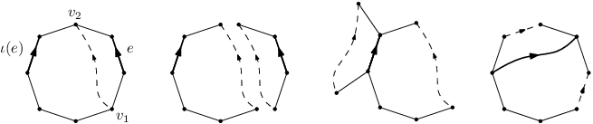
Thus, by successively adding and erasing edges to and , we may arrive at a point where . Then, by Proposition 11.8, there exists a homeomorphism of which sends to . ∎
12. Riemannian metrics
12.1. Measured and Riemannian marked surfaces
In the setting of Markovian holonomy fields, the scale of time is provided by a means to measure areas on each surface that one considers.
Definition 12.1.
Let be a smooth compact surface. A measure of area on is a smooth non-vanishing density on , that is, a Borel measure which has a smooth positive density with respect to the Lebesgue measure in any coordinate chart.
A gluing is a diffeomorphisms outside a negligible subset. Hence, a measure of area on a surface determines a measure of area on any other surface obtained by splitting this surface along a curve.
Definition 12.2.
Let be a smooth compact surface endowed with a measure of area denoted by . Let be a mark on and let be the surface obtained by splitting along . Let be the associated gluing. Then is a measure of area on which we denote by .
On an oriented surface, a measure of area is also the same thing as a non-vanishing differential -form. We are going to work with surfaces endowed with a specific measure of area, on which we will choose Riemannian metrics. We would like these two structures to be compatible. In fact, we have the following result.
Proposition 12.3.
Let be a marked surface. Let be a measure of area on . There exists a Riemannian metric on whose Riemannian volume is and such that the curves of are closed geodesics.
Before we prove this proposition, let us state a definition.
Definition 12.4.
A marked Riemannian surface is a quadruple , where is a marked surface endowed with a smooth density and is a Riemannian metric on with Riemannian volume and such that the curves of are closed geodesics.
Proof.
In this proof, we denote by the Riemannian volume of a Riemannian metric on . Let us first assume that is orientable and has no boundary. We write .
Let be any Riemannian metric on . Let be the smooth real function on such that . Set . The Riemannian volume of is .
For each , let denote a neighbourhood of diffeomorphic to such that corresponds to . We assume that are pairwise disjoint. For each , we denote by the natural coordinates in .
Let be a smooth function such that and . Let be the smooth real function on defined by
For each , consider the Riemannian metric in and set
Finally, define by The Riemannian volume of coincides with outside the set . Moreover, the total volume of is the same for and . Finally, are geodesic for .
For each , and all , set . It is understood that when . Similarly, set . The functions and are both smooth, increasing, equal to at and they coincide on . Define a diffeomorphism of by setting
The metric satisfies . Hence, the volume of any cylinder , is the same for and for . Moreover, since preserves the curves , they are still geodesic for .
Let and be the two smooth functions defined on such that and . For each , define
By construction of , we have for each and all the equality . It is easy to check that the mapping from to itself defined by
is a diffeomorphism. Set . Then by construction, and give the same volume to any subset of which is a rectangle in the coordinates . Hence, they agree on , hence on . Since preserves the curves , they are still geodesic for . Thus, has the desired properties.
Let us explain how the result extends to surfaces with boundary and non-orientable surfaces. Let be a non-orientable surface without boundary. Then there exists an orientable double of , that is, an orientable surface and a smooth mapping which is a covering of degree . This surface can for instance be constructed as the unitary frame bundle of the real line bundle for some Riemannian metric on . The density and the marks of can be lifted through . This yields an orientable marked surface endowed with a density whose total area is equal to twice that of . The result that we have proved above applied on yields a Riemannian metric with Riemannian volume and such that the curves of are geodesics. Let be the non-trivial automorphism of the covering , that is, the diffeomorphism of which exchanges the sheets of the covering. Then the Riemannian metric has Riemannian volume and makes the curves of geodesics. Since the equations of geodesics are linear in the metric, the curves of are also geodesic for the metric . This metric has also Riemannian volume . Moreover, it is invariant by , hence descends to a Riemannian metric on with the desired properties.
Finally, if has a boundary, then we may glue a disk along each boundary component of and extend to a measure of area on the surface without boundary thus obtained. ∎
12.2. Partially ordered sets of graphs
The set of graphs on a compact surface carries a natural partial order.
Definition 12.5.
Let be a topological compact surface. Let and be two graphs on . We say that is finer than and write if .
It is straightforward that is finer than if and only if . The inclusion implies but the converse is false.
As a poset, the set of graphs on a surface has few good properties. In particular, it is not directed, which means that it contains pairs without upper bound.
Lemma 12.6.
Let be a topological compact surface. The set of graphs on endowed with the partial order is not directed. In other words, there exist two graphs and on such that no third graph satisfies and .
Proof.
Let be an open subset of identified through a homeomorphism with the disk of centred at the origin and of radius 2. Let and be the parametrized curves defined by
For all , let denote the open domain of delimited by the restrictions of and to . The sets are also the bounded connected components of the complement of the union of the ranges of and in the plane.
The curves and are edges, so by Lemma 11.7, there exist two graphs and on such that is an edge of and is an edge of . Assume that there exists a graph such that and . Then would contain the union of the ranges of and . Since the range of an edge has an empty topological interior, none of the sets would be contained in . Hence, would have infinitely many faces. We have observed after Proposition 11.8 that this is impossible.∎
This fact will be a serious problem for us at a later stage. A better-behaved substitute for the set of graphs is the set of graphs with piecewise geodesic edges.
Definition 12.7.
Let be a marked surface endowed with a Riemannian metric . We define as the set of graphs on with piecewise geodesic edges, that is
The set can be non-empty only if the marks on are geodesic curves. We know by Proposition 12.3 that it is always possible to choose a Riemannian metric on for which this is the case.
The next result states that is indeed a better set of graphs than the set of all graphs.
Proposition 12.8.
Let be a marked surface endowed with a Riemannian metric for which the marks are geodesic curves. Any finite family of piecewise geodesic paths on is a subset of for some graph on with geodesic edges.
In particular, the poset is directed.
Proof.
We have observed after the definition of a graph (Definition 11.2) that there exists a graph on with geodesic edges. Now, by induction on the number of curves in the finite family of curves that we consider, it suffices to prove that, given a piecewise geodesic path and a graph with geodesic edges, there exists a graph with geodesic edges such that .
For this, let us subdivide into a product of geodesic edges in such a way that each edge either is contained in one edge of or has its interior contained in the interior of a face. By adding finitely many vertices to , which means subdividing some of its edges, we produce a new graph which is such that each which is contained in an edge of is an edge of . Each other has its interior contained in a single face of . By lifting the curves to a split pattern of , we reduce the problem to the case of a finite collection of geodesic segments contained in the interior of a disk with piecewise geodesic boundary. In this case, since the skeleton of contains the boundary of the disk, it follows from Proposition 11.10 that any pre-graph obtained by adding edges to and whose skeleton is connected is a graph. Thus, it suffices to join one endpoint of each of the curves to a point on the boundary of the disk by a geodesic segment and then to add a vertex at every point where two distinct geodesic curves meet. Hence, can be refined into a graph with geodesic edges such that belong to .
In order to prove that is directed, consider two graphs and with piecewise geodesic edges. The property that we have just proved applied to provides us with a graph which is finer than both and . ∎
12.3. Approximation of graphs
In this section, we prove that any graph can be approximated in a strong sense by a sequence of graphs with piecewise geodesic edges. We start by defining the lasso decomposition of a piecewise geodesic path, which is a variant of the more familiar operation of loop-erasure. Recall the definition of equivalence of paths and lassos (see Section 11.4).
Proposition 12.9.
Let be a Riemannian compact surface. Let be an element of such that . There
exists in a finite sequence of lassos with meanders and an
injective path with the same endpoints as such that
1. ,
2. .
If is a loop, the same decomposition holds with the single difference that is a
simple loop. In both cases, we call the loop-erasure of and denote it by .
Proof.
By Lemma 12.8, we may assume that is a path in a graph. By adding vertices to this graph, we may also assume that no edge of this graph is a simple loop. Let us write as a product of edges: . We proceed by induction on . If , then is its own loop-erasure. Now assume that . If is not reduced, that is, if it contains at least one sequence , then we reduce it. This can only shorten . Now set . This is the first time at which hits itself. Assume that with . By definition of , is uniquely determined by this relation. Set , and . Then . By construction, is a simple loop and is a path shorter than with the same endpoints. Moreover, . The result follows. ∎
Proposition 12.10.
Let be a marked Riemannian surface.
Let be a graph on . Let be a real number.
There exists a graph on with piecewise geodesic edges and two bijections and , denoted by the same letter, such that the following properties hold.
1. .
2. The bijection commutes with the inversion and preserves the endpoints : for all ,
, and .
3. The bijection induced by is such that for all , .
4. For all , and for all , .
Notice that it is not possible to simply take for some large . Indeed, the new edges thus produced may behave badly near the vertices. For example, several edges may form a complicated spiral near a vertex that they share. In this case, it is neither certain that their loop-erased dyadic piecewise geodesic approximations do not intersect each other nor that they leave the vertex in the same cyclic order as the original edges.
If and is smaller than the injectivity radius of , we denote by the segment of minimizing geodesic joining to .
Proof.
Let be the injectivity radius of . Let be such that the balls are pairwise disjoint, an edge meets a ball only if is an endpoint of , and the cyclic order of the outcoming edges at every vertex is the cyclic order of their last exit points from the ball for all . The existence of such an is granted by Lemma 11.16. Let us choose an orientation of each ball .
For all real and all , define . Observe that . Define
The path is the concatenation of three injective paths which meet only at their endpoints, so that it is injective. Thus, is an edge with the same endpoints as . Let and be two edges such that . The central portions of and are contained in and respectively, so that they are disjoint. By the assumption made on , they do not enter any ball . Hence, and meet, if at all, in one of these balls and this can occur only at one of their endpoints.
Let be an edge. The continuity and injectivity of imply that as . Since , this implies that tends to as tends to . Moreover, one always has the inequality .
Let be fixed. Let be an integer such that for all , . For all integer , define
The path is piecewise geodesic, with the same endpoints as , but it may not be injective, even for large . On the other hand, it coincides with near its endpoints, more precisely, on a segment of length at least . When tends to infinity, converges to . We claim that for all such that , the paths and intersect only at some of their endpoints for large enough. Indeed, consider for all the segment
Choose such that . Choose such that . For all , and are respectively contained in the sets and , whose intersection is the same as the intersection of and .
For each integer , choose such that for all . Then choose such that for all . Set . Then for each , the sequence converges to with fixed endpoints, and satisfies . For each and each , set . We claim that a subsequence of the sequence tends to when tends to infinity.
Indeed the sequence is uniformly bounded in length by . Hence, the paths being parametrized at constant speed, it is relatively compact in the uniform topology and we can extract a sequence which converges uniformly to a path . The image of is contained in the image of and it joins to . Hence, the images of and coincide. In particular, . Using the lower semi-continuity of the length with respect to the uniform convergence, we find
It follows from these inequalities that converges to , hence to , as tends to infinity. Let us choose a subsequence such that the convergence holds for each edge and define for all .
For all and all , is a piecewise geodesic edge with the same endpoints as . Moreover, by construction, . If is geodesic, then . Finally, the set is the set of edges of a pre-graph on . By Corollary 11.12, is in fact the set of edges of a graph on , which we denote by .
By construction, the bijection between and preserved the cyclic order at every vertex of . Let us apply Proposition 11.22. Since , the graph satisfies all the desired properties for large enough. ∎
Chapter 2 Multiplicative processes indexed by paths
In this chapter, we begin the study of the class of objects to which Markovian holonomy fields belong: stochastic processes indexed by paths on a compact surface and with values in a compact Lie group which satisfy a condition of multiplicativity. We discuss the canonical space of such processes, two distinct -fields on it, and prove the version of Kolmogorov’s theorem that is best suited to our situation. We then study a kind of uniform measure on the canonical space, thus providing the first example of what will be called in the next chapter a discrete Markovian holonomy field. We conclude by constructing a set of generators of the group of reduced loops in a graph for which we are able to determine the finite-dimensional marginal of the uniform Markovian holonomy field.
From now on, the expression compact surface will mean smooth compact surface.
13. Multiplicative functions
Let be a group, on which we make for the moment no assumption at all.
Definition 13.1.
Let be a compact surface. Let be a subset of . A function is said to be multiplicative if for all such that and for all such that and . The set of multiplicative functions from to is denoted by .
For an explanation of the reversed order in this definition, see the introduction, Section 5.
The gauge group is the symmetry group of the physical theory from which our objects are issued.
Definition 13.2.
The group of all mappings from to is called the gauge group of and it acts by gauge transformations on the space , as follows. If belongs to and belongs to , then is defined by
More generally, given a subset of , the group acts on in the same way, where is defined as the set of endpoints of the paths of .
Example 13.3.
Assume that are simple loops based at the same point of . Write . The concatenation of two loops of is never a simple loop, hence never an element of . If we assume moreover that the inverse of a loop of is never in , then any -valued function on is multiplicative, so that . The action of the gauge group on is simply the action of on by simultaneous conjugation of each factor. This fundamental example should be kept in mind when one reads Lemma 13.5. It explains the importance of this action of in our context.
We cannot do much if we do not make a few assumptions on . For the rest of this section, we assume that it is a compact topological group. We do not assume that it is connected, so that it can in particular be finite. Also, for the moment, we do not assume that it is a Lie group. The group carries its normalized Haar measure and we denote simply by the integral of a function with respect to this measure.
Let be a subset of . The object of this paragraph is to discuss two natural -fields on . The simplest one is the cylinder -field, denoted by , which is defined as the smallest -field which makes the evaluation mapping measurable for all . The gauge group acts by bi-measurable transformations and it makes sense to speak of measures on which are invariant under gauge transformations.
It is also natural to consider a smaller -field which consists in events which are invariant under the action of the gauge group. In order to discuss this -field, let us first associate an abstract graph to each subset of .
Definition 13.4.
An abstract graph is a pair of finite sets , whose elements are called vertices and edges, endowed with two mappings , called respectively source and target.
Let be a subset of . The configuration graph of is the abstract graph defined by setting , and, for each , and .
In what follows, we will make use of the diagonal adjoint action of on defined by .
Lemma 13.5.
Let be a compact surface. Let be a subset of . Assume that is stable by concatenation and inversion, and the configuration graph of is connected. Let be a vertex of this configuration graph. Let be elements of . Let be a continuous function such that the function is gauge-invariant on . Then there exists loops in all based at and a continuous function invariant under the diagonal action of such that
Proof.
Consider the configuration graph of . If it is not connected, let us choose one vertex in each connected component not containing and add to the collection a path of joining to this vertex. That such a path exists follows from the assumptions made on . The collection has become for some . We denote the configuration graph of this enlarged collection by .
Let be a spanning tree of . For each , the path is a loop based at . When written as a product of edges, it becomes a word in and this word makes sense as an element of . More precisely, it is a loop of based at , which we denote by .
Let be an element of . Let us define a gauge transformation by setting if and, for all , . If is an edge which belongs to , then it is easy to check that . Hence, for all , and, by the invariance property of , .
Choose . Since the loops are all based at , the action of the gauge transformation defined by if and transforms into . Let us define by
Then and is invariant under the diagonal action of . The result is proved. ∎
This result motivates the following definition.
Definition 13.6.
Let be a subset of stable by concatenation and inversion. The invariant -field on , denoted by , is the smallest -field such that for all , all integer , all finite collection of loops based at and all continuous function invariant under the diagonal action of , the mapping is measurable.
If can be written as the disjoint union of and which are both stable by concatenation and inversion and whose configuration graphs are disjoint, then is canonically isomorphic to and the invariant -filed on is the tensor product of the invariant -fields on and .
Let and be two surfaces. Let be a smooth mapping. Let be a subset of and . Then induces a map from to , hence a map from to .
Lemma 13.7.
Let and be two surfaces. Let be a smooth mapping. Let be a subset of and . Then the induced map is measurable with respect to the cylinder -fields, and also with respect to the invariant -fields.
Proof.
Let be continuous and consider . The function on is equal to the function , which is measurable with respect to because belongs to . This proves the first assertion.
Now let be continuous and invariant under the diagonal action of by conjugation. Let be loops of based at the same point. Then are loops of based at the same point and the function on is measurable with respect to . This proves the second assertion.∎
Let us conclude this paragraph by discussing the case of a graph. Let be a surface endowed with a graph . Let be an orientation of . It is plain that a multiplicative function on is determined by its values on the edges or even just those of . More precisely, the natural surjective mapping induced by the inclusion is one-to-one. Indeed, if belongs to , then for some and . Then, for all multiplicative function , one has .
Since the interior of an edge contains no vertex, the concatenation of at least two edges is never an edge. Hence, every mapping from to is multiplicative. We will often make the identifications
without further comment. In particular, we will sometimes use a collection of elements of to denote an element of .
Proposition 13.8.
Let be a compact surface endowed with a graph . Let be a vertex of . Let be a generating subset of the group of reduced loops in based at . The invariant -field on is generated by the functions of the form where is continuous and invariant by diagonal conjugation.
Proof.
By definition of the invariant -field and by Lemma 13.5, it suffices to prove that for all and all continuous invariant by diagonal conjugation, the function can be put under the form for some invariant function . This is easily done by expressing, modulo the equivalence relation on paths, the loops as words in the generators . One then uses the multiplicativity of the elements of and the fact that the multiplication map is equivariant with respect to the diagonal actions of by conjugation. ∎
14. Multiplicative families of random variables
Let be a compact surface and a subset of . A probability measure on determines a family of -valued random variables which are just the evaluation functions on , defined by . These random variables form a multiplicative family in the sense that and almost surely whenever this makes sense. If is countable, then the converse is true since one can dismiss the negligible event on which the equalities do not hold. We prove in this section that the converse is in fact true even if is not countable. Let us recall the definition of a projective family of probability spaces.
Definition 14.1.
A projective family of probability spaces is the data of the following ingredients.
A partially ordered set .
For each , a probability space .
For each pair such that , a measurable mapping .
These ingredients are assumed to satisfy the following conditions.
1. The poset is directed : for all , there exists such that and .
2. For all such that , one has the equality .
3. For all such that , one has .
Let us state a general result of existence and uniqueness.
Proposition 14.2.
We keep the notation of Definition 14.1. Let denote the set-theoretic projective limit of the family , endowed for each with the canonical mapping . Let denote the smallest -field on which makes all the mappings measurable.
Assume that for each , is a compact metric space endowed with the Borel -field. Assume also that for all such that , the mapping is continuous.
Then there exists a unique probability measure on such that for all , one has .
This result belongs to a wide family of theorems whose prototype is due to Kolmogorov and whose common ground is Caratheodory’s extension theorem. The most common versions assert the existence and uniqueness of under less restrictive conditions on the probability spaces but more restrictive conditions on the poset. Typically, is a subset of a finite-dimensional Euclidean space and the probability spaces are Polish space. The form which we have stated is in fact fairly easy to prove due to the strong assumptions which we make on the probability spaces. We think wiser to give a proof than to refer to several places in the literature from which the reader would have to collect the various pieces of the argument.
Proof.
Let denote the Cartesian product of the sets , . Recall that the set-theoretic projective limit of the family is, by definition, the set
The set , endowed with the product topology, is a compact topological space of which , as intersection of closed sets, is a compact topological subspace. It is endowed with the continuous coordinate mappings , .
For each , let denote the closed support of the probability measure . It is a non-empty compact subset of . Consider . The equality implies that . We claim that for all , . Indeed, choose and . Define, for all , . Then on one hand, . On the other hand, the discussion above implies that no finite intersection of the sets is empty. Since these sets are compact, their intersection is non-empty. Hence .
Define a collection of subsets of by setting . The collection is not a -field, but it is stable by complementation, finite unions and finite intersections. Consider . Assume that and for some and , . Let be such that and . Then . Since , this equality implies . Hence,
We have proved that implies . Hence, for all , it is legitimate to call the common value of all for and such that . Thus, we have defined . It is not difficult to check that is finitely additive.
We claim that is -additive on . In order to prove this, it is sufficient to prove that if is a decreasing sequence of elements of such that , then . Let us choose such a sequence . Let us also choose . For each , let us write for some and some . For each , the inner regularity of the measure implies the existence of a compact subset of such that . Since endowed with the trace of the product topology of is compact, the sets , are compact. Since for all , the intersection is empty. Hence, there exists such that . Now, for each , there exists at least one such that , so that . Hence, . This proves that tends to 0 when tends to infinity.
Carathéodory’s extension theorem asserts that admits a unique -additive extension to the -field generated by , which is by definition the smallest -field on such that the mappings are measurable. This extension of , which we still denote by , satisfies for all by definition. ∎
In our setting, this theorem can be applied as follows.
Proposition 14.3.
Let be a subset of . Let be a collection of finite subsets of whose union is and which, when ordered by the inclusion, is directed. For all , let be a probability measure on . Assume that the probability spaces endowed with the restriction mappings defined for form a projective system. Then there exists a unique probability measure on such that for all , the image of by the restriction mapping is .
In particular, if is a collection of -valued random variables such that
1. ,
2. ,
then there exists a unique probability measure on such that the distribution of the canonical process under is the same as the distribution of .
Proof.
Let be elements of such that . Then is a compact subset of , actually a smooth compact submanifold. The evaluation mappings on generate both the topology and the -field . Hence, is the Borel -field. Moreover, the restriction mapping is continuous.
Proposition 14.2 ensures the existence of a probability measure on the projective limit of the sets underlying our probability spaces, endowed with a certain -field. In the present case, the projective limit of the sets is easily identified with the set in such a way that the mappings are simply the restrictions. Through this identification, the -field on which Proposition 14.2 constructs a measure is the usual cylinder -field. The first assertion follows.
Let be a collection of random variables which satisfies the assumptions 1 and 2. For each finite subset of , the distribution of is a Borel probability measure on , which we denote by and which is actually supported by . By applying the first assertion to the collection of probability spaces where spans the collection of finite subsets of , we find the desired probability measure on . ∎
15. Uniform multiplicative functions on a graph
Let be a compact surface. Let be a graph on . In this paragraph, we discuss the uniform measure on and some of its natural disintegrations. The disintegrations that we have in mind are associated with random variables associated to marking curves or boundary components. Before we define the measures, let us set up some notation.
15.1. Constraints on marked surfaces
Let us denote by the set of conjugacy classes of . The inversion map on descends to an involution of which determines an action of on . Recall that if is a marked surface, then acts on by reversing the orientation.
Definition 15.1.
Let be a marked surface. A set of -constraints on is a -equivariant mapping .
A set of -constraints on a marked surface determines a set of -constraints on any splitting of this surface. In the case of unary splittings, we need the following observation. If is a conjugacy class of , then the set of squares of elements of is also a conjugacy class, which we denote by .
Definition 15.2.
Let be a marked surface endowed with a set of -constraints. Consider . Let be the elementary gluing with joint . The marked surface carries the set of -constraints defined by for all , with the following exception: if is a unary gluing and , then .
Consider a marked surface with -constraints. Given , we say that satisfies the constraints if
| (21) |
The set of elements of which satisfy the constraints is globally invariant under the action of the gauge group.
15.2. Uniform measures
Definition 15.3.
Let be a compact surface. Let be a graph on . Let be an orientation of . The Haar measure on , seen as a probability measure on , is called the uniform measure and denoted by .
Plainly, the uniform measure does not depend on the choice of . The reason for the subscript will become apparent soon. We would like now to incorporate boundary conditions and constraints along marking curves into the uniform measure .
Let be a conjugacy class. Let be an integer. The set
is a -homogeneous space under the action
Let denote the extension to of the unique -invariant probability measure on . In particular, and is the -invariant probability measure on , which we also denote simply by . For each element of , we denote by the conjugacy class of .
Lemma 15.4.
Consider , , and a continuous map . Let be a conjugacy class of . The following relations hold.
| (22) |
| (23) | |||||
| (24) |
| (25) |
| (26) |
Proof.
The right-hand side of (22) defines a measure supported by and invariant under the action of . Hence, it is . The relation (23) follows easily from (22). The right-hand sides of (24) and (25) are equal to
for all . The relation (24) follows because the map maps into , and (25) also follows because the set is stable by circular permutation of the variables. The relation (26) follows also from this description of and a simple change of variables. ∎
Let be a marked surface with a set of -constraints, endowed with a graph . Let us choose simple loops in which represent the unoriented cycles of , that is, such that . Recall that for the sake of simplicity, we denote in the same way a cycle and the corresponding simple loop. We label the elements of in such a way that for . Let be an orientation of such that for all and . Let us label the other edges of .
Lemma 15.5.
Let be a marked surface with -constraints. Let be a graph on . The uniform measure on with -constraints is defined as the probability measure
It is denoted by . The corresponding probability measure on , also denoted by , depends neither on the choice of the simple loops which represent the marking of nor on the choice of .
Proof.
The invariance of the measures by cyclic permutation of the variables, granted by (25), ensures that the measure does not depend on the simple loops which we have chosen to represent the cycles of the marking of . Since the Haar measure on is invariant by inversion, the measure induced on by does not depend on the choice of . ∎
Let us state two basic properties of the measure .
Proposition 15.6.
Recall the notation of Lemma 15.5.
1. The event
satisfies .
2. The action of the group on preserves the
probability measure .
Proof.
1. By definition of , the support of is contained in the closed set .
2. Choose and . Set if and . If is not located on a curve of , then the translation invariance of the Haar measure implies that leaves the measure invariant. Assume now that is on the curve which is represented by the cycle . Assume that is outcoming at and is incoming. Then the action of translates the variables associated to the edges adjacent to other than and and it replaces by . This leaves the measure invariant. Finally, the action of preserves the measure . Since the group is generated by elements which are equal to at all vertices but one, the result follows. ∎
Let us state precisely the fact that the measures disintegrate each other.
We use the notation . This set does not include the boundary components of anymore. Let us define and for each , . For each , any collection of conjugacy classes of determines the set of -constraints on which maps on for all . We denote this set of constraints simply by .
The following lemma is a direct consequence of the definition of and (26). It shows that the measures provide a regular disintegration of with respect to the random variables .
Lemma 15.7.
Let be an integer between and . Let be conjugacy classes of . Let be a continuous function. Then
| (27) | |||||
| (28) |
15.3. Surgery of uniform measures
Let us investigate the behaviour of the uniform measures that we have just defined under the basic operations of surgery. So far, we have used the letter to denote gluing maps and also test functions on . In the proof of the next result, we need to use both. This is why we change our notation for gluings.
Proposition 15.8.
Let be a marked surface with -constraints endowed with a graph . Let be a splitting of and let denote the gluing map. Let be the graph on obtained by lifting . Then the mapping induced by satisfies
| (29) |
In this proposition, it is crucial that we consider the invariant -fields, not only for the general reason that one should consider only gauge-invariant quantities, but because the equality (29), although meaningful with cylinder -fields thanks to Lemma 13.7, would simply be false. For instance, consider a binary gluing along two curves and with joint . Then the event belongs to and has measure zero. On the other hand, the pull-back by of this event is the event of which has full measure. The point is that the first event does not belong to .
Proof.
Let be a continuous function invariant under the action of . Then induces a continuous function and we need to prove that the following relation holds.
| (30) |
We treat separately the cases of binary and unary gluings.
1. Binary gluing – Let be the joint of the gluing. Let and be the two boundary components of which are identified by , oriented in such a way that .
Let , and denote respectively the set of edges located on , and . These three sets are naturally identified by the gluing. Set and . The gluing identifies naturally with . With this notation, we have the partitions
| (31) |
The partition of above determines the equality , according to which we denote by the generic element of . Similarly, we have the decomposition and we write for the generic element of .
With this notation and these identifications, the function is defined by the equality .
Since each curve of is covered either by or by , the decomposition of above determines a decomposition of the measure as the tensor product of two measures and on and respectively, each of which is invariant under the action of the gauge group . Let us assume that is the product of edges of . Then can be identified with and the measure corresponds to under this identification.
Similarly, the measure splits as the tensor product of three measures , and , on , and respectively. The last two spaces can be identified with and the measures and correspond to under this identification.
The measures and correspond to each other via the identification of and . Hence, the equality which we need to prove is the following:
Let denote the subset of consisting of the vertices which lie on . The group is a compact Lie group and the invariant measure of its transitive action on the subset of is the measure . Let us denote by the generic element of and by the Haar measure on this group. Since is invariant under the action of the gauge group, we have for all in the equality . Observe that some edges of have some of their endpoints in , so that the term is affected by the gauge transformation . On the contrary, the term is not affected because and are disjoint. Hence, with the identifications made earlier,
Since the measure is invariant under the action of , the last term is equal to
It suffices now to prove an equality about the function on . Indeed, let us denote this function by . All we need to prove is that, for all conjugacy class ,
But the left-hand side is equal to
hence to the right-hand side.
2. Unary gluing – Let be the joint of the gluing. Let be the component of the boundary of such that . Let us write and in such a way that for all .
Let denote the set of edges located on . Set and . Set and . We will identify freely with .
With this notation, the equalities (31) hold, as well as the subsequent decompositions of and . The function is also still defined by the equality .
The decomposition is valid just as in the binary case, but the decomposition of is now different. Indeed, this measure splits into the tensor product of and a measure on which is under the natural identification of with . The formula which we need to prove is the following:
Let denote the set of vertices which lie on . By using the invariance of under the action of the subgroup of the gauge group and the invariance of the measure under the same action, we find just as in the binary case that the left-hand side of the equality to prove is equal to
The notation here is misleading, since the two occurrences of do not denote the same object. Indeed, the two occurrences of in the arguments of are identified respectively with an element of and an element of , on which acts differently.
Now what we have to prove is really an equality about the function
on . Let us call this function . We need to prove that for all conjugacy class in the following equality holds:
Recall that is the conjugacy class constituted by the squares of the elements of . We claim that this equality holds for all continuous function . Indeed, the integral
is the integral of with respect to the measure , by the very definition of this measure as the invariant measure under the natural action of on . Hence, by a simple particular case of (23), the integral that we are computing is equal to
The measure is equal to for -almost all . Hence, the measure between the brackets is . This concludes the proof. ∎
Let us conclude this section by a much simpler result, which is the simplest instance of invariance under subdivision.
Proposition 15.9.
Let be a marked surface with -constraints. Let and be two graphs on . Assume that . Then the inclusion induces a measurable restriction map which satisfies
Proof.
Let us choose an orientation for and . The restriction map, seen as a map from to , multiplies the components which correspond to the edges of which constitute each edge of and forgets about the components which correspond to edges which do not lie in the skeleton of .
Since the product of independent uniform variables on is still uniform, the only non-trivial thing to check is what happens along the marking curves or the boundary components. There, the invariance follows from (24). ∎
16. Tame generators of the group of reduced loops
Consider a surface with -constraints along its boundary, endowed with a graph . Our objective in this section is to exhibit a family of lassos which generates the group of reduced loops in and to compute the distribution of the -valued random variables associated with these lassos under the constrained uniform measure defined in the previous section. Moreover, we are going to do this in a way which is consistent with the partial order on the set of graphs.
Definition 16.1.
Let be a compact surface endowed with a graph . Let be a vertex of . A lasso is said to be facial if its meander represents a facial cycle of . It is said to be bounding if its meander covers a connected component of .
We want to prove the existence of systems of generators of which consist in one bounding lasso for each connected component of , one facial lasso for each face of , and as many supplementary lassos with non-contractible meander as the genus of (see Section 9.1).
Recall the notation from Section 11.5. If is a word in some set of letters, we denote by the word obtained by reversing the order of the letters of .
Proposition 16.2.
Let be a connected compact surface. Let denote the reduced genus of . Let be the number of connected components of . Write . If is oriented, we assume that bound positively. Let be a graph on . Let be a vertex of . Let denote the number of faces of .
1. There exists, in the group , lassos ; bounding lassos whose meanders are equivalent to up to permutation; facial lassos whose meanders bound the faces of , positively if is oriented; and there exists an word in the letters which belongs to such that the group admits the presentation
and, for all continuous function and all set of -constraints along the boundary components of ,
where we have set .
A collection of lassos such as will be called a tame system of generators associated with the word .
2. Let and be two graphs on such that . Set . Let be a vertex of . Let be a tame system of generators of associated with the word . Assume that the faces of are labelled in such a way that for all , the meander of the lasso bounds . For all , let be the set of faces of contained in and set .
Then there exists a set of facial lassos in such that for all , the meander of the lasso bounds a face of , for all the equality holds and
is a tame system of generators of associated with the word .
We will use the notation , , and until the end of this chapter.
By Lemma 11.33, we know that is free of rank . By Euler’s relation for the graph , which writes , the rank of can also be written as . In order to find families of generators whose cardinal decomposes naturally as , we introduce the dual graph of .
Definition 16.3.
Let be a compact surface endowed with a graph . Let be a split pattern of . Let denote the set of connected components of , which is in canonical bijection with . Then, set . For each element of , define the source of as the connected component of which contains and the target of is the connected component of which contains .
The abstract graph is called the dual graph of .
Properly speaking, the dual graph of depends on the choice of the split pattern of and it is unique only up to an obvious notion of isomorphism. We shall in fact choose a split pattern and work with the associated dual graph.
The involution of the split pattern induces an involution on , which we still denote by . This involution is similar to an orientation reversal, but one should observe that it may have fixed points. For example, if an edge is sent by on a boundary component of , then and the dual edge also satisfies .
The orbits of on , which we call unoriented edges of the dual graph, correspond bijectively by with the unoriented edges of the graph , that is, the pairs for .
Definition 16.4.
Let be a compact surface endowed with a graph . Let be a split pattern of . Recall that a spanning tree of the dual graph is a subset stable by the involution and such that any two vertices of the dual graph are joined by a unique injective path made with edges of .
Let be a spanning tree of the dual graph. An orientation of is said to be adapted to if for all , the edges and are neither both positively oriented nor both negatively oriented with respect to this orientation of .
Assume that is endowed with an orientation adapted to . Then we define the image by of an edge of as an edge of by setting if is positively oriented as a subset of and otherwise.
It is not difficult to check that there are exactly two orientations of , among the possible, which are adapted to any given spanning tree in the dual graph. Moreover, for all , we have the equality in .
It follows from Proposition 11.15 that is the set of edges of a graph on with a single face. This graph has edges, so by Euler’s relation, it still has vertices. Moreover, its skeleton contains and every edge of which lies on is also an edge of . Let be a collection of edges comprising exactly one edge on each connected component of . If is oriented, we assume that the edges of bound positively. The set of edges of located on and which do not belong to form a cycle-free subgraph of . Hence, it is possible to extend this subgraph to a spanning tree of such that (see Figure 12).
Lemma 16.5.
With the notation above, for each edge , the lasso is a bounding lasso whose meander covers the connected component of on which lies and whose spoke contains no edge lying on this connected component.
Proof.
Let be the connected component of on which lies. If the base point is located on , then is a simple loop which represents the cycle . Otherwise, since any two vertices located on can be joined by a path in which stays in , there exists a unique vertex on which is joined to the base point by a path in with no edge lying on . Hence, . The three paths between the brackets form the meander of the lasso, which is a simple loop covering . ∎
Let us carry on with our construction. We have a partition , where . It follows from Euler’s relation that contains exactly unoriented edges. From the fact that has vertices, we deduce that is in fact a spanning tree of . Hence, Lemma 11.33 implies the first assertion of the following result.
Proposition 16.6.
Let be a compact surface endowed with a graph . Let be a split pattern of . Let be a spanning tree of the dual graph of . Let be a collection of edges comprising exactly one edge on each connected component of , which we assume to be positively oriented if is oriented. Set . Let be a spanning tree of such that . Set . Choose an orientation of such that . Write . Let be the boundary components of enumerated in such a way that for all , is the meander of the lasso . Then , and contain respectively , and edges and the following properties hold.
1. The group is freely generated by the loops .
2. Under the probability measure on , the collection of random variables is a collection of independent variables. For all , the variable is uniformly distributed on and for all , the variable has the distribution .

Proof.
Let us prove the second assertion. By definition of the measure , the random variables are independent, uniformly distributed on , and independent of . Hence, the variables are independent, uniformly distributed and independent of the variables , which do not involve any edge of .
Now choose . Consider the loop and the corresponding bounding cycle . By Lemma 16.5, the spoke of the lasso does not involve any edge lying on the boundary component of . However, it may involve edges located on other boundary components of .
We claim that for every subset , there exists such that for all , the spoke of does not involve edges located on . Assume to the contrary that for some subset there does not exist such an . Then there would exist all distinct and such that for all , the spoke of the lasso involves an edge which lies on the boundary component . This would in particular imply that for each there exists a path in from to and, since , that contains a cycle.
By relabelling the boundary components of , we may assume that for all , the element of the subset has the property described above. Since under , the random variable has the distribution and is independent of the variables for not located on , the variable itself has the distribution and is independent of . This implies easily the result. ∎
With the proof of Proposition 16.2 in mind, the next step is to express the loops for in function of facial lassos. The exact way in which these lassos decompose into products of facial lassos depends on, and in fact encodes completely, the geometry of the tree .
Let be endowed with an orientation adapted with . Let be a vertex of which corresponds to a face . The set of edges of whose source is is in one-to-one correspondence with the set of edges of located on the boundary of and which bound it positively. This set carries a natural cyclic order, which is the order in which the edges are traversed by a cycle bounding . By restriction, the set of edges of which share as their source is endowed with a cyclic order.
Let us root by not only choosing a reference vertex but also by choosing among the edges issued from this vertex which one is the first. The simplest way to do this is to choose a vertex of . This determines a root vertex for , namely the connected component of which carries this vertex, and this also breaks the cyclic symmetry of the edges issued from this connected component, which are now totally ordered.
The object that we are now contemplating is a tree (that is, an abstract graph without simple cycle) endowed with a distinguished vertex, a total order on the edges issued from this distinguished vertex and a cyclic order on the set of edges issued from any other vertex. Such an object is called a rooted planar tree and it has a canonical representation as a set of words of integers, according to a formalism due to J. Neveu. Let us simply describe how the vertices are labelled by words of integers, that is, finite sequences of non-negative integers.
The root vertex is labelled by the empty word . Let be the number of children of , that is, the number of vertices to which it is joined by an edge. These vertices are labelled by words of length 1, namely , according to the total order on these edges.
Then, consider a vertex labelled by a word . The integer is called the height of and it is denoted by . Let denote the predecessor of and let denote the number of vertices other than to which is joined by an edge. Then the edge from to , denoted by , breaks the cyclic symmetry among the edges issued from and determines a total order on the other edges issued from . The targets of these edges are labelled in this order.
Thus, the choice of a rooting of and an adapted orientation of determines a labelling of by words of integers (see Figure 13). As we shall see now, it determines also a specific facial lasso for each face of and one of the loops for each face distinct from the root face.

Definition 16.7.
Let be a compact surface endowed with a graph . Let be a split pattern of . Let be a spanning tree of the dual graph of . Endow with an orientation adapted to . Choose a root for . Label the faces of with words of integers accordingly.
Consider a face of labelled by the word . If , let be the unique representative of which starts at the root vertex chosen in and bounds positively . Otherwise, consider the edge of , which we identify with an edge of which bounds positively. Let be the unique simple loop representing which starts with this edge. Write as a product of edges . We define the facial lasso by .
Consider a face distinct from the face labelled by . The edge of determines the edge of and we define . We also define as the constant loop at .
Let and be two vertices of . We say that is a prefix of if there exists a word of integers such that , the concatenation of and . Genealogically, this can be phrased by saying that is an ancestor of .
Lemma 16.8.
Recall the notation of Definition 16.7. Let be a face of labelled by . There exist elements of the subgroup of generated by such that
| (32) |
Moreover, there exists an element of the subgroup of generated by and such that
| (33) |
Proof.
Let us write . By definition, is the edge of which corresponds to the edge of . Hence, . Then, the list consists of the images by of the edges of which join to , in this order, intermixed with some edges of and some edges of . The claimed expression for follows. In the case where is the root of , the edge does not play a special role, it is either the image by of the edge which joins to in , or an edge of .
We say that a vertex of is a leaf if . The second expression of reduces to the first if is a leaf. Let us now consider a vertex and assume that (33) holds for each vertex of which is the predecessor, that is, for . For every vertex , the fact that is a prefix of for some implies that is a prefix of . Hence, by applying (32) to and then (33) to , we find that (33) holds for .
By induction along , the second expression of holds for all . ∎
Corollary 16.9.
Proof.
Let us call the height of and denote by the maximal height of a vertex of , which is necessarily a leaf. We claim that for all integer , is freely generated by the set defined by
For , it is the statement which we wish to prove. For , it is the content of Proposition 16.6. The fact that the claim is true for all is easily proved by descending induction. Indeed, for all , the set is deduced from by replacing, for all labels of such that , the loop by the facial lasso . If is a basis of , then it follows immediately from (33) that is another basis of .
Since the sets are disjoint for the distinct labels of height , the assertion on the distribution of the variables follows easily from (33) and the distribution of . ∎
At this point, we have proved most of the first assertion of Proposition 16.2. We have exhibited a family of generators of the group which generate it freely. We know that if we add one element to this family, we get a presentation of with one relation. The next result helps us to get a relation of the form that we expect.
Lemma 16.8 defines for each ordered pair of adjacent vertices in , and also an extra element . Now for each pair of vertices of , not necessarily adjacent, let us define , where is the unique injective path in from to .
Lemma 16.10.
Endow the set of vertices of with the lexicographic order associated to the reversed order on . Enumerate its elements accordingly: . Then
| (34) |
Moreover, the loop is the boundary of the unique face of . It is equal to a word in the lassos where each lasso of the set appears exactly twice, possibly sometimes with exponent , and each lasso of the set appears exactly once, possibly with exponent . If is oriented, then each lasso of the set appears with exponent .
Proof.
The equation (32) can be rewritten as
Let us apply this relation to . We find
| (35) |
Let us define, for all integer and all vertex of such that an element of by setting
Also, for each , let be the vertices of of height at most listed in the lexicographic order corresponding to the reversed order on . Then (35) can be written as
By applying (32) iteratively to the terms of the form in this equality, one finds that the equality
holds for all . Here, has the meaning explained before the statement of Lemma 16.10. For larger than the height of , this formula is exactly what we wanted to prove.
Finally, is the product of the loops where goes around the unique face of the pattern of obtained from by sewing the edges of . The result follows. ∎
We are now ready to prove the main result of this section.
Proof of Proposition 16.2.
Let us consider the relation given by Lemma 16.10. Let us define, for all ,
Then the relation (34) becomes
| (36) |
By Corollary 16.9, is freely generated by and, under , the variables are independent, uniformly distributed and independent of .
Let us write . By the last part of Lemma 16.10, there exists elements of the subgroup generated by , signs , and a permutation such that
with if is oriented.
By Lemma 16.10 again, the loop can be written as a word in where each loop appears exactly twice, possibly sometimes with exponent . Let us name the loops and let denote the element of the free group of rank such that . Let us also define, for all , . Then the relation (36) becomes
| (37) |
2. Let us prove the second assertion. By adding vertices to , we do not change the group nor the distribution of the associated random variables, according to Lemma 15.9. Hence, we may add to the vertices of located on and, without loss of generality, assume that .
For the sake of simplicity, let us treat the case where only one face of contains the interior of an edge of . Once the result is proved under this restrictive assumption, the general result follows by iteration.
Let us assume that only the face contains the interior of some edges of . The choice of the face is a simple matter of convenience, we do not use anything specific to this face.
Let be a split pattern of . Let be the closure of the preimage by of . Let be the restriction to of the lift to of . Let be the finishing point of the spoke of the lasso . Let us choose a vertex of which is sent by on .
The first assertion of the proposition that we are proving applied to the graph on the disk , whose reduced genus is , provides us with facial lassos based at which bound the faces of and such that such that bounds . By projecting these lassos on by and conjugating them by the spoke of , we get lassos based at which we denote by .
Let denote the tame set of generators of that we are given. Let us prove that the set of loops obtained by replacing by in is a set which generates . Let be a loop based at in . Let us split into a concatenation of paths which are either paths in or concatenation of edges of . We get an expression of the form , where the paths are in and the paths are concatenations of edges of . Choose and consider the path . It can be lifted in a unique way to a path in , which we denote by . Even if is a loop, needs not be a loop. However, there exist two paths and in which stay on the boundary of and such that is a loop based at . Let us write and , and denote the spoke of the lasso by . Finally, let be a path in from to . We have the equality in
The loops between brackets are loops of and the loops between square brackets are the image by of loops in , conjugated by the spoke of , hence, equal to words in the loops . Hence, the loops of generate . They satisfy the equation
In particular, the set for instance has cardinal and generates which is free of rank . Hence, it is a free basis of this group (see Proposition 2.7 in Chapter 1 of [26]).
There remains to determine the distribution of under . It follows from the way in which the loops were constructed that the random variables are independent, uniformly distributed, and independent of . Moreover, is independent of . Hence, the three -fields
are independent. Since and are uniformly distributed, and , it follows that are uniformly distributed and independent of . ∎
Chapter 3 Markovian holonomy fields
In this chapter, which is the core of this work, we define Markovian holonomy fields and their discrete analogues. We prove in full generality that the partition functions of a discrete Markovian holonomy field do not depend on the graph in which they are computed. We then prove the first main result of this work, which asserts that any discrete Markovian holonomy field which satisfies some regularity conditions can be extended in a unique way to Markovian holonomy field.
17. Definition
Definition 17.1.
A measured marked surface with -constraints is a quadruple where is a marked surface, is a smooth non-vanishing density on and is a set of -constraints on .
Two measured marked surfaces (resp. orientable measured marked surfaces) with -constraints and are isomorphic if there exists a diffeomorphism (resp. an orientation preserving diffeomorphism) such that , sends each curve of to a curve of and, for all , .
From now on, we will make the assumption that is a compact Lie group, not necessarily connected. If , we endow with a bi-invariant Riemannian metric which we normalize in such a way that the Riemannian volume of is 1. In this way, the Riemannian density coincides with the normalized Haar measure on . If is finite, we endow it with the distance and with the uniform probability measure.
The set of conjugacy classes of inherits the quotient topology from and the corresponding Borel -field. The space of -constraints on a marked surface , which we denote by , is a subset of and thus carries the trace topology and -field.
Let us introduce some more notation. Let be a measured marked surface with -constraints. Let be a curve which belongs to . Let be an element of . We define a new set of -constraints as follows: we set , and on . The main definition of this work is the following.
Definition 17.2.
A -valued two-dimensional Markovian holonomy field is the data,
for
each quadruplet consisting of a marked surface endowed with a density and a set of
-constraints, of a finite measure on such
that the following properties are satisfied.
A1. For all , .
A2. For all and all event in the invariant -field of
, the function is a measurable function on the set .
A3. For all and all ,
A4. Let be a homeomorphism such that , and . Let be loops based at the same point on . Assume that their images by are also rectifiable loops. Then, for all continuous function invariant under the diagonal action of by conjugation,
In particular, if is a diffeomorphism, then the mapping from
to induced by sends the measure
to the measure .
A5. For all and , one has the identity
A6. For all , all and all gluing along , one has
A7. For all and for all ,
A -valued two-dimensional oriented Markovian holonomy field is the data, for each quadruplet consisting of an oriented marked surface endowed with a density and a set of -constraints, of a finite measure on the measurable space such that the seven properties above are satisfied.
It is important to notice that the measures are not probability measures in general. They are finite measures, whose masses carry a lot of information about the holonomy field. It is actually possible that they characterize it completely, but this is a question which has yet to be answered.
Let us discuss briefly the significance of these axioms. The axioms A1, A2 and A3 express the fact that the measure , seen as a function of the -constraints, provides a regular disintegration of with respect to the value of the holonomy field along the curves of . The simple expression of A3 is permitted by the fact that we consider finite measures rather than probability measures. The axiom A4 expresses the invariance of the field under area-preserving diffeomorphisms. The axioms A5 and A6 express the Markov property of the field. Finally, A7 is a normalization axiom. Without it, if was a given Markovian holonomy field, then for any real , the measures would constitute another Markovian holonomy field.
Our purpose is not to study Markovian holonomy fields in full generality. In the rest of this paper, we are going to make strong regularity assumptions and investigate the corresponding fields.
Recall that denotes a bi-invariant distance on . Let and be two paths with the same endpoints. Then, although and are not measurable with respect with the invariant -field , unless and are loops, the function is -measurable, because it can also be written as and is a loop.
Definition 17.3.
Let be a -valued two-dimensional Markovian holonomy
field.
1. We say that
is stochastically continuous if, for all and for all sequence
of elements of which converges with fixed endpoints to ,
2. We say that is Fellerian if, for all , the function
defined on is continuous.
3. We say that is regular if it is both stochastically continuous and Fellerian.
In the definition of stochastic continuity, we use convergence of -valued random variables. Since is compact, this is equivalent to convergence in probability and to convergence in for any .
From now on, the expression (regular) Markovian holonomy field will stand for two-dimensional -valued (regular) Markovian holonomy field.
18. Discrete Markovian holonomy fields
It is not easy to construct a Markovian holonomy field. Indeed, one has to construct a stochastic process indexed by loops. To do this, one must naturally specify the finite-dimensional marginals of this process. Thus, to each finite collection of loops, one has to associate a probability measure on some power of . But unlike points on a time interval, loops on a surface may form a very complicated picture. In fact, in most cases, it is impossible to determine a probability measure from a finite set of loops. A way around this problem is to start by describing a restriction of the process to a class of loops which are nice enough, like piecewise geodesic loops, and then to extend the process by continuity. In fact, the very first step is to build a process indexed by the set of loops in a graph for every graph on a surface. This is what we call a discrete holonomy field.
Definition 18.1.
A -valued two-dimensional discrete Markovian holonomy field is the data, for each measured marked surface with -constraints, and each graph on , of a finite measure on such that the following properties hold.
D1. For all and all , .
D2. For all , all and all event in the invariant -field of
, the function is a measurable function on .
D3. For all , all and all ,
D4. Consider and , endowed respectively with and . Let be a homeomorphism. Assume that , , and . Then the mapping from to induced by satisfies
D5. For all and , endowed respectively with two graphs and one has the identity
D6. For all , all , all and all gluing along , one has
D7. For all , all and all ,
DI. For all , all and graphs on such that , the restriction map satisfies
A -valued two-dimensional discrete oriented Markovian holonomy field is the data, for each oriented measured marked surface with -constraints and all graph on , of a finite measure on such that the properties above are satisfied.
The axiom DI is specific to discrete holonomy fields. It is an axiom of consistency and is usually called the property of invariance under subdivision.
Lemma 18.2.
Any (oriented) Markovian holonomy field determines a discrete (oriented) Markovian holonomy field.
Proof.
For all surface endowed with a graph , the set is a subset of . Hence, a Markovian holonomy field determines by restriction a discrete Markovian holonomy field, except perhaps for the axiom DI. In fact, this axiom is satisfied by the restriction of a Markovian holonomy field because the finite dimensional marginals of a stochastic process constitute a consistent system of probability measures. ∎
Our main goal in this chapter is to prove a result in the other direction and to extend, when it is possible, a discrete holonomy field to a continuous one. For the moment, let us discuss briefly the discrete holonomy fields for themselves. It turns out that we have already constructed a fundamental example of discrete Markovian holonomy field.
Proposition 18.3.
The family of measures is a discrete Markovian holonomy field. We call it the uniform -valued discrete holonomy field.
Proof.
The measure is a probability measure on the cylinder -field of . By restriction, it defines a measure on the invariant -field. The axiom D1 is satisfied by Proposition 15.6. By Proposition 13.8 and the definition of the measures , it is possible to write as an expression which is explicitly measurable with respect to the -constraints. Hence, the axiom D2 is satisfied. Axiom D3 is satisfied by (26). That axioms D4, D5 and D7 hold is straightforward. Axiom D6 is satisfied thanks to Proposition 15.8. The invariance property DI holds by Proposition 15.9. ∎
This discrete Markovian holonomy field is very special in that is consists only in probability measures.
Definition 18.4.
Let be a collection of finite measures as in Definition 18.1, which does not necessarily satisfy any of the axioms listed in this definition. To each and each graph , we associate the number
which is called the partition function.
We have said earlier that these numbers carry a lot of information about the field. A crucial property is that they do not depend on the graph .
Proposition 18.5.
Let be a collection of finite measures as in Definition 18.1, which satisfies the axioms D4, D5, D6 and DI. Consider and two graphs and on . Then
| (38) |
If there exists a graph such that and , then the equality (38) is a straightforward consequence of the axiom DI. Unfortunately, by Lemma 12.6, the set of graphs on is not directed and such a graph does not always exist.
Proof.
By Proposition 9.12, it is possible to split along each of the curves of . Thus, there exists a measured surface with -constraints and no marks and a gluing whose joint is . We can lift to a graph on and the axiom D6 enforces the equality . Since we can do the same for the graph , it suffices to prove the result when . Then, the axiom D5 implies that the partition function associated to (resp. ) is the product of the partition functions associated to the connected components of endowed with the corresponding restrictions of (resp. ).
Hence, it suffices to prove the result when is connected and . In this case, the axiom DI implies that we can remove or add edges to , in the sense of Propositions 11.15 and 11.26, without altering the partition function.
By Proposition 11.36, by such transformations we can go from to a graph which is sent to by a homeomorphism of . By D4, this implies the result. ∎
Let be a discrete holonomy field. In order to produce a Markovian holonomy field from , the first natural step is to apply Proposition 14.2 to put together the measures which associates to a directed subset of the set of graphs on a surface. For this, we need to consider Riemannian metrics.
Let be a Riemannian marked surface (see Definition 12.4). The axiom DI and Proposition 14.3 imply that the collection of the measures , where spans the set of graphs with piecewise geodesic edges, determines a finite measure on , where is the set of piecewise geodesic paths on .
Definition 18.6.
Let be a discrete holonomy field. Let be a Riemannian measured marked surface with -constraints. The finite measure on obtained by taking the projective limit of the measures where spans is denoted by .
At this point, there are two things to do. Firstly, one needs to extend the measure to for all and secondly, one needs to prove that the result of this procedure would have been the same with another Riemannian metric. The first step requires some regularity from the holonomy field.
Definition 18.7.
Let be a discrete holonomy field. We say that is stochastically -Hölder continuous if the following property holds.
Let be a Riemannian marked surface with -constraints. Then there exists a constant such that for all graph on and all simple loop with bounding a disk ,
Our unique example so far of a discrete holonomy field, the uniform holonomy field, does unfortunately not satisfy this property. Indeed, it assigns uniform random variables to arbitrary small simple loops. We will construct other more regular discrete holonomy fields later.
The second step of the program outlined above requires another regularity condition, which is more global but less quantitative.
Definition 18.8.
Let be a discrete holonomy field.
1. We say that is continuously area-dependent if the following property holds.
Let be a marked surface with -constraints. Let be a sequence of graphs on . Let be a sequence of homeomorphisms of . Assume that for all and, for all face of , tends to as tends to infinity.
Then, denoting by the induced map , we have the weak convergence
2. We say that that is Fellerian if for all measured marked surface , the mapping which to a set of -constraints associates the number is continuous on .
3. We say that is regular if it is stochastically -Hölder continuous, continuously area-dependent and Fellerian.
It is tempting to conjecture that a stochastically -Hölder continuous discrete Markovian holonomy field is continuously area-dependent. At least, the two properties are not equivalent, as our unique example so far shows. For the moment, let us state our main result concerning the construction of Markovian holonomy fields.
Theorem 18.9.
Every regular discrete Markovian holonomy field is the restriction of a unique regular Markovian holonomy field.
The proof of this theorem occupies the rest of this chapter.
19. An abstract extension theorem
The core of the proof of Theorem 18.9 is the next result, which we formulate in a way which is mostly independent of the context of Markovian holonomy fields.
Theorem 19.1.
Let be a compact Riemannian surface. Let denote the Riemannian volume of . Let be a complete metric group on which translations and inversion are isometries. Let be a multiplicative function. Assume that there exists such that for all simple loop bounding a disk and such that , the inequality holds.
Then admits a unique extension to an element of , also denoted by , such that if a sequence of paths converges with fixed endpoints to a path , then .
Let us state right now the application of this theorem to the extension of holonomy fields.
Corollary 19.2.
Let be a stochastically -Hölder continuous discrete Markovian holonomy field. Let be a Riemannian marked surface with -constraints. There exists a unique probability measure on whose image by the restriction mapping is the measure and such that for all sequence of paths which converges with fixed endpoints to a path , one has
Proof.
The canonical process on can be seen as a mapping from to the set . In general, the set of -valued random variables on any probability space is a group for the multiplication of random variables. The metric makes it a complete metric space. Both structures are compatible in that the product and inverse mappings are continuous. Moreover, the translations and the inversion map are isometries.
The assumption of stochastic Hölder continuity ensures that the regularity condition is satisfied by the family . Hence, we can apply Theorem 19.1. It produces a family of random variables which is multiplicative and continuous with respect to the convergence of paths with fixed endpoints. Proposition 14.3 applied to this family asserts that there exists a probability measure on under which the canonical process has the distribution of .
The uniqueness of the measure follows from Proposition 10.12 which asserts that is dense in for the convergence with fixed endpoints. ∎
The rest of this section is devoted to the proof of Theorem 19.1. A basic tool for this proof is the lasso decomposition of a piecewise geodesic path (see Proposition 12.9).
Proposition 19.3.
Under the assumptions of Theorem 19.1, there exists a constant such that for every loop with , .
Proof.
Assume first that is a simple loop. If is small enough, then bounds a disk, which we denote by . Moreover, a local isoperimetric inequality holds on : if is small enough, say , then for some constant . Then, if denotes the constant given by the assumptions of Theorem 19.1, . The result is proved in this case.
Let us now treat the general case. Let us apply Proposition 12.9 to find the lasso decomposition of . By the multiplicativity of , which is part of the assumptions of Theorem 19.1, . Since the distance on is invariant by left translations and inversion, we have
Hence, . By Proposition 12.9, and the result follows. ∎
This result tells us that if is a simple piecewise geodesic loop close to the constant loop, then is close to the image by of the constant loop. Our next generalizes this statement to the case of a piecewise geodesic path which is close to a geodesic segment.
Proposition 19.4.
Under the assumptions of Theorem 19.1, there exists a constant such that the following property holds. Let be a segment of minimizing geodesic. Let be a piecewise geodesic path with the same endpoints as . Assume that . Then
The assumptions imply that is shorter than . If we take , then is a loop and we recover the estimate of Proposition 19.3.
In order to prove this proposition, we use a decomposition result similar to the lasso decomposition and the following isoperimetric inequality. Needless to say, the constant which appears in this Euclidean case is not optimal.
Lemma 19.5.
Let be real numbers. Let be a rectifiable Jordan curve of length in the Euclidean plane such that a piece of this curve is a segment of length . Then the area of the bounded component of satisfies the inequality
Let be a compact Riemannian surface. There exists a constant such that the following property holds. Let be a rectifiable Jordan curve of length such that a piece of this curve is a segment of minimizing geodesic of length . Then the area of the smallest disk bounded by satisfies the inequality

Proof.
The Riemannian case can easily be deduced from the Euclidean case by working in normal coordinates at one end point of the geodesic part of . The compactness of ensures that the resulting distortions of lengths and areas are bounded.
Let us consider the Euclidean case. Under the constraints on , is maximal when is the concatenation of a segment of length and an arc of circle of length . In this case, let be the radius of this circle and the angle under which the arc of circle is seen from the centre of the circle. Then and . Now one has the relations
| (39) | |||
| (40) |
One checks easily that for all , . Hence, (40) implies , and since , we have . Combining this with (39), we find
This is the expected result. ∎
The generalization of the lasso decomposition that we need is the following.
Proposition 19.6.
Let be a Riemannian compact surface. Let be a geodesic segment on and an injective piecewise geodesic path with the same endpoints as . It is possible to decompose and as concatenations and in such a way that, for each , or is a simple loop. In particular, if we set , then is a lasso and .
Proof.
Consider the set . It is a reunion of isolated points and closed subintervals of . Let be the reunion of these isolated points and the end points of these intervals. The set contains the two end points of . Set . Then dissects both and into edges: and .
For each , define by the relation . Since is injective, the mapping from to itself is one-to-one. Hence, it is a permutation. We look for the records in the sequence . Define and write . Set . Observe that . Set . For each , set and . By construction, and .
Choose and consider . Assume first that . Then . Either this edge is contained in , in which case , or it meets only at its endpoints, which are also those of . In this case, is a simple loop. Assume now that . We claim that any point of other than one of its end points which is located on is in fact located on one of the edges . Indeed, if this was not the case, there would exist such that is located on between and . But then we would have which contradicts the definition of . Hence, in this case, is a simple loop.∎
We are now ready to prove Proposition 19.4.
Proof of Proposition 19.4.
Assume that and are shorter than the bound of Proposition 19.3. Let be the loop-erasure of . By the properties of the lasso decomposition of (Proposition 12.9) and Proposition 19.3,
Now we are reduced to consider which is an injective path. Let and be the decomposition given by Proposition 19.6. We have
where is the area enclosed by . By Lemma 19.5 and since ,
By Hölder inequality, it follows that
Hence,
∎
The estimate given by Proposition 19.4 will allow us to associate an element of to every element of . Recall the definition of the dyadic piecewise geodesic approximation of a path (Definition 10.11). For a given path , is in general only defined for larger than a certain integer . Nevertheless, by Proposition 10.12, the sequence converges to in 1-variation.
Proposition 19.7.
Let . Under the assumptions of Theorem 19.1, the sequence is a Cauchy sequence in .
Proof.
Let be the constant given by Proposition 19.4. Let be an integer such that . Choose . Write according to the notation of Definition 10.11. Write also , where for each , . By Proposition 19.4, for all , Hence, by Hölder inequality, and since ,
The result follows now from the fact that converges to . ∎
By Proposition 19.7 and the assumption that is complete, it is now legitimate to set the following definition.
Definition 19.8.
For each , we define by
Proposition 19.9.
The mapping thus defined is continuous at fixed endpoints.
Notice that we have not proved yet that is continuous even on .
Proof.
Take and consider a sequence in converging to with fixed endpoints. We claim that converges to . An elementary argument shows that this implies the continuity of with fixed endpoints on .
Choose . Choose an integer such that . Such an integer exists by definition of . Now for each and each , let be the geodesic segment joining to . If , let us also denote by the portion of parametrized by the interval . Observe that and are constant paths. The simple equivalence
implies the following inequality:
where is the decomposition given by the definition of . The path is piecewise geodesic and shares the same endpoints as the segment . Hence we can apply Proposition 19.4 to find
By Hölder inequality again,
Since converges to and tends to 0, the right hand side tends to zero as tends to infinity. For large enough, it is smaller than . For such , . ∎
Remark 19.10.
The factors in the last expression are very unpleasant, because they give the feeling that is not uniformly continuous on . In fact, the last proof reveals that, on endowed with the distance , is uniformly continuous on subsets where converges uniformly to . It is likely that a much better result can be achieved by considering the stronger distance on . Ideally, one could expect to be -Hölder continuous on . I have not been able to prove or disprove this statement.
20. Extension of discrete holonomy fields
Let be a Riemannian marked surface with -constraints. Starting from a discrete Markovian holonomy field satisfying a regularity condition, we have constructed a measure on (see Corollary 19.2). The construction of this measure involves a Riemannian metric and we must now prove that the result is independent of this choice. We start by identifying the distribution of under for an arbitrary graph .
Proposition 20.1.
Let be a stochastically -Hölder continuous and continuously area-dependent discrete Markovian holonomy field. Let be a Riemannian marked surface
with -constraints. Let be a graph on . Recall the notation from Corollary 19.2.
1. The distribution of under is .
2. The measure does not
depend on the Riemannian metric . We denote it by .
3. The distribution of
under is .
Proof.
1. For each , let be the graph produced by Proposition 12.10 with . Let denote the corresponding bijection. By the stochastic continuity of the process under , which follows from Theorem 19.1, the distribution of is the limit of the distributions of the families as tends to infinity.
Since preserves the cyclic order at each vertex of , there exists for each a homeomorphism of which preserves and which sends on and which induces the bijection . Let be such a homeomorphism. Since for each face of , the boundary of is , the face is .
Moreover, the distribution of the family under is the distribution of the same family under , hence the distribution of under , where denotes the map induced by from to .
By the fourth assertion of Proposition 12.10, tends to as tends to infinity for all . Hence, the assumption that is continuously area-dependent implies that the distribution of the family under converges weakly to as tends to infinity.
2. Let and be two Riemannian metrics on . By Lemma 12.8 and the property that we have just proved, the distributions of under and agree. Since is dense in for the convergence with fixed endpoints (see Proposition 10.12), the continuity property granted by Theorem 19.1 implies that .
3. This property follows immediately from the first two. ∎
We can now finish the proof of the main theorem of this section.
Proof of Theorem 18.9.
Let be a regular discrete Markovian holonomy field. By applying Corollary 19.2 and Proposition 20.1, we get for all measured marked surface with -constraints a finite measure on which by restriction produces a measure on the invariant -field. The total mass of the measure is the common value of the masses of the measures for all graph on , which we have denoted by . In particular, this mass is finite.
Now, we check that the seven axioms of Definition 17.2 are satisfied. We choose a measured marked surface with -constraints . We endow with a Riemannian metric and use without further comment the fact, granted by Proposition 20.1, that .
A1. Let denote the event . Let be a graph on . By Proposition 20.1 and the axiom D1 for ,
A2. The set of bounded measurable functions from to whose integral against depends measurably of the -constraints is a vector space which contains the constant functions and is stable by uniformly bounded monotone limit. Thus, by a monotone class argument, and by definition of the invariant -field , in order to show that this space contains all bounded functions measurable with respect to , it suffices to show that it contains all functions of the form where are loops based at the same point and is continuous and invariant under the diagonal action of by conjugation.
Let us choose and as above. For each and all large enough, let denote the dyadic piecewise geodesic approximation of of order . Let us define a function and a sequence of functions on the set of -constraints on as follows :
and, for all ,
Our goal is to prove that the function is measurable. For all , the fact that converges to with fixed endpoints implies, according to the conclusion of Theorem 19.1, that converges in probability to , so that tends to as tends to infinity. Hence, it suffices to prove that is measurable for large enough. In fact we claim that is continuous as soon as it is defined. Indeed, for each , can be computed in a piecewise geodesic graph. There, the dependence in can be made explicit and all functions in the integrand are continuous. The result follows.
A3. Just as in the last point, it suffices to check the equality when it integrates a function of the form , where are piecewise geodesic and is invariant by diagonal conjugation. Hence, it suffices to prove the equality for for any graph with piecewise geodesic edges. In this last case, the property follows from the axiom D3 satisfied by .
A4. The metric is a Riemannian metric on in the sense of Proposition 12.3. We need to prove that the image measure of by the mapping induced by is . Again, we may restrict ourselves to functions of the form , where are piecewise geodesic, hence to the discrete measures associated to graphs with piecewise geodesic edges. Let be a graph on with piecewise geodesic edges. Then , the graph constituted by the images by of the edges of , is a graph on with piecewise geodesic edges and, by the axiom D4 for , the distribution of under is the same as the distribution of under . The property follows.
A5, A6 and A7 follow respectively from the axiom D5, D6 and D7 satisfied by and the same approximation argument as in the previous points.
The fact that the new Markovian holonomy field is stochastically continuous is a part of the conclusion of Theorem 19.1. Finally, the Feller property follows from the Feller property of . ∎
Chapter 4 Lévy processes and Markovian holonomy fields
In this chapter, we apply the extension theorem proved in the previous chapter to construct a whole family of Markovian holonomy fields. Before that, we study the partition functions of an arbitrary regular Markovian holonomy field and prove that they are completely determined by a Lévy process on the group with some nice properties, essentially a continuous density. We then construct a Markovian holonomy field for each such Lévy process. The case of the Brownian motion on a connected Lie group yields the Yang-Mills measure.
21. The partition functions of a Markovian holonomy field
In this section, we establish some fundamental properties satisfied by the masses of the finite measures which constitute a Markovian holonomy field.
To start with, we describe the isomorphism classes of connected surfaces with -constraints on the boundary. If is oriented, we denote by the subset of which consists in the curves which have the orientation induced by that of .
Proposition 21.1.
Let and be two connected measured marked surfaces with -constraints. If and are orientable, we assume that they are oriented. They are isomorphic if and only if the following
conditions hold simultaneously.
1. and are homeomorphic.
2. .
3. If and are oriented, there exists a bijection such that
on .
3’. If and are non-orientable, there exists a -equivariant bijection
such that .
We use this result to associate to every Markovian holonomy field a family of functions of one or several variables in .
Let be a Markovian holonomy field. Let and be two non-negative integers, with even. Let be a positive real number. Recall the notation of Section 9. Let be a surface homeomorphic to , endowed with a density of total area . Let denote the positively oriented connected components of . Let be elements of . Let be the unique set of -constraints on such that, for all , . By Proposition 21.1 and the axiom A4, the number depends on , and only through , the unordered list and the fact that is orientable. Hence, it is legitimate to set
This defines a symmetric function of conjugacy classes of . If the Markovian field is Fellerian, then this function is continuous with respect to . If , is just a number, namely the total mass of the measure where is the connected sum of tori endowed with a density of total area .
Similarly, let and be two integers, respectively positive and non-negative. Let be a surface homeomorphic to , endowed with a density of total area . Let denote the disjoint connected components of endowed with an arbitrary orientation. Let be elements of . Let be the unique set of -constraints on such that, for all , . When is not oriented, we define
Again, if , is just the total mass of the measure where is the connected sum of projective planes endowed with a density of total area .
Definition 21.2.
Let be a Markovian holonomy field. The functions
where spans , are called the partition functions of the field .
In the rest of this section, we fix a Markovian holonomy field and study its partition functions. They are infinitely many but the Markov property of the field implies that they satisfy an infinite set of relations and that they are in fact completely determined by a small number of them.
Let us introduce several operations on functions of conjugacy classes of . Firstly, we identify functions of a conjugacy class of and functions on which are constant on the conjugacy classes. Thus, we may speak of continuous or integrable functions of a conjugacy class. This point of view is consistent with our previous definition of a topology and -field on (see Section 17). Of particular interest is the space of square-integrable functions of one conjugacy class of , which we identify with the space of conjugation-invariant square-integrable functions on . If is an integer, we identify the elements of the -th symmetric tensor power with symmetric functions of conjugacy classes. We use the shorthand notation for .
Definition 21.3.
For all integers and , the three linear mappings , and are defined by
| (41) | |||||
| (42) |
and, for all and all ,
| (43) |
We will now use these linear mappings to formulate the relations between the partition functions of the holonomy field. The operation expresses the transformation of the partition function under a unary gluing, and the contractions and correspond to binary gluings, respectively of two boundary components which lie on the same connected component of the surface and two boundary components which lie on two distinct connected components.
Recall that we use the notation for with the following meaning : if and in all other cases.
Proposition 21.4.
Let
be the partition functions of a Markovian holonomy field .
1. For all , all integers and
all real , the function is square-integrable with respect to any of
its variables for any value of the other.
2. The following equality holds:
| (44) |
Moreover, if , then
| (45) |
Finally, for all , all and all real , the following equality holds:
| (46) |
Proof.
Let us start by proving the second assertion. Choose as above. It follows from the axiom A2 that is a measurable function. Since it takes non-negative values, the integral which defines is well defined, possibly infinite. Let us prove that the identity (44) holds.
Let be a surface homeomorphic to , endowed with a surface measure of total area . Consider and let be a unary gluing along , with joint . Thus, . The surface is not orientable and it has boundary components. According to the observation made after Definition 9.10, it is homeomorphic to the connected sum of a projective plane and the surface obtained by gluing a disk along one boundary component of . Thus, it is homeomorphic to . Finally, induces on a surface measure with total area .
Let be a set of -constraints on . Applying axioms A3 and then A6 gives us the relation
Recall from Definition 15.2 that, since we are considering a unary gluing, puts the constraint on . Translating the last relation in terms of the partition functions gives (44).
The proofs of the relations (45) and (46) are very similar. For the relation (45), one considers a binary gluing in which one identifies two boundary components of a connected surface. If the surface is orientable, the two boundary components are identified by an orientation-reversing diffeomorphism. The result of this gluing can be described as the connected sum of a torus and the surface obtained by gluing two disks along two boundary components of the original surface. Thus, it has two boundary components less, and reduced genus increased by . For the relation (46), one considers a binary gluing in which one identifies two boundary components located on two distinct connected components of a surface. Proposition 9.4 settles the issue of orientation and reduced genus of the resulting surface.
The assertion of square-integrability follows from (45) and (46) as we shall see now. Firstly, observe that Theorem 9.7 and the axiom A4 imply that the value of a partition function is not affected by simultaneously replacing each argument by its inverse. Now, for all ,
The last number is indeed finite and the assertion is proved. ∎
Corollary 21.5.
The partition functions of a Markovian holonomy field are completely determined by the functions and .
Proof.
For all non-negative and , such that is even and , the following identity holds:
| (47) |
Then, the equalities
| (48) |
determine all non-orientable partition functions. Finally, the equality
determines the only remaining partition function. ∎
An important consequence of Proposition 21.4 is that for all , the function is the density with respect to the Haar measure of a measure on . By the axiom A7, it is a probability measure. In the next proposition, we start to study the behaviour of these probability measures as tends to , under the assumption that the holonomy field is stochastically continuous. Recall that we denote by the unit element of and that we use the notation for the unique -invariant probability measure on .
Proposition 21.6.
Let be the partition functions
of a
stochastically continuous Markovian holonomy field. Then, as tends to 0, one has the following
weak convergences of measures on .
1. .
2. .
Proof.
1. Let be the disk of radius 1 centred at the origin in endowed with the Lebesgue measure, which we denote by . We denote by the positively oriented boundary of . For each , let be the path which goes straight from the origin to the point and let be the loop based at which goes once counterclockwise around the circle of radius centred at the origin. For all , we denote by the canonical process on , we consider the measure on and we denote by the corresponding expectation. Let be a continuous invariant function on . We compute . By the multiplicativity property of , it is equal to . By the axiom A3, we can disintegrate this expectation with respect to the value of . We find
We use now the axioms A6 and A5 to split along and we find
By integrating over and using the axiom A7, we find
| (49) |
Our goal is now to prove that the left-hand side tends to as tends to . For this, we use the stochastic continuity of the holonomy field. Indeed, as tends to 0, the loop converges with fixed endpoints to the constant loop at the origin. Hence, for all , as tends to . By the multiplicativity of and the fact that , the mapping is identically equal to 1. Hence, . In order to integrate this convergence with respect to , we use the fact that
and the right-hand side is continuous, hence integrable, with respect to . Hence, the dominated convergence theorem applies and we deduce that the left-hand side of (49) tends to as tends to 0.
2. Let be the closed disk of radius 4 centred at the origin in from which one has removed the two open disks of radius 1 centred respectively at the points and . We endow with some density denoted by . Let (resp. ) be the loop which starts at (resp. ) and goes once around the circle of radius 1 centred at (resp. ), counterclockwise. Let be the path which goes straight from to . Choose . Consider the union of the two closed disks of radius centred at and and the rectangle . Let be the loop which starts at and bounds this domain with positive orientation. Let be the path which goes straight from to . As tends to 0, the loop converges with fixed endpoints to the loop . However, in order to apply our axioms, we need to replace by a loop based at the same point and whose image is a smooth submanifold of . We do this in such a way that the convergence of to is preserved.
We consider the measure on , where is characterized by the fact that , and maps the circle of radius 4 centred at the origin to . We denote the corresponding expectation by . Let be a continuous invariant function on . For all , we have
where is the area of the domain delimited by , and and is the total area of . By the same arguments as in the previous proofs, the left-hand side converges as tends to 0 to and the convergence is dominated with respect to . Since the two endpoints of are distinct and the measure is invariant under gauge transformations, the distribution of is both left and right-invariant on . Thus, has the uniform distribution on . Hence, By integrating with respect to , we find
∎
We will use this result to prove that the partition functions a stochastically continuous Markovian holonomy field are completely determined by the functions . Let us introduce two probability measures on .
Definition 21.7.
Let and be the two invariant probability measures on defined respectively by the fact that for all continuous function on ,
| (50) |
The letters and correspond to the words handle and cross-cap. We start by proving some important properties of these measures.
Let denote the set of isomorphism classes of irreducible representations of over . Given with character and a measure on , the Fourier coefficient is defined by . Recall that an irreducible representation is said to be complex if its character is not real valued, otherwise real (resp. quaternionic) if it preserves a non-degenerate symmetric (resp. skew-symmetric) complex bilinear form.
If is a measure on , we denote by the measure defined by . By an invariant measure we mean a measure which is invariant by conjugation.
Lemma 21.8.
Let be three invariant probability measures on . If for every complex representation , then . In particular, . Moreover, .
Proof.
The Fourier coefficients of and can be computed easily by using the elementary theory of characters:
The Fourier coefficients of the convolution product of two measures is given by the relation . Moreover, the Fourier coefficients of are the complex conjugate of those of . Hence, on real and quaternionic representations, whose character is real, the Fourier coefficients of are real and agree with those of . Hence, and have the same Fourier coefficients. Since they are both invariant, they are equal. The equality follows immediately. The last assertion is proved by computing the Fourier coefficients of both sides. ∎
Remark 21.9.
We invite the reader to compare the equality with the fact that the connected sum of a projective plane and a torus is homeomorphic to the connected sum of three projective planes (or the connected sum of a projective plane and a Klein bottle).
In the next proposition, we use the notation for the integral of a function against a measure and we denote by the convolution of probability measures.
Proposition 21.10.
The partition functions of a regular Markovian holonomy field are completely determined by the functions for . One has the following explicit formulas.
For all , all even, all and all , one has
| (51) |
Moreover, for all , all , all and all , one has
| (52) |
Proof.
Let us start by proving (51) when and , by induction on . For , it is a consequence of the fact that is invariant by conjugation. Assume that and the result has been proved for . Then, for all and all , (46) yields
Since the Markovian holonomy field that we consider is Fellerian, the function
is continuous on the compact set . Hence, when tends to , it converges uniformly as a function on towards . Thus, using the convergence proved in Proposition 21.6, we find
Using the induction hypothesis, we find
because is already an invariant measure on . This is the expected result.
Let us now treat the case where . We have
The result follows now from the equality which one checks easily using the elementary properties of the Haar measure.
It is now easy to complete the result obtained in Proposition 21.6. We leave the proof of the following corollary to the reader.
Corollary 21.11.
Let be the partition functions
of a regular Markovian holonomy field. Then, as tends to 0, one has the following
weak convergences of measures on .
1. For all , all even and all ,
2. For all , all and all ,
22. The Lévy process associated to a Markovian holonomy field
In the previous section, we have reduced the description of the partition functions of a regular Markovian holonomy field to the description of the one-parameter family of functions , . This allows us to state a classification result.
Proposition 22.1.
Let be a regular Markovian holonomy field. Then the probability measures on are the one-dimensional distributions of a unique conjugation-invariant Lévy process issued from the unit element. If the Markovian field is not oriented, then the distribution of this Lévy process is invariant by inversion. Moreover, this Lévy process determines completely the partition functions of .
It is conceivable that a regular Markovian holonomy field is completely determined by its associated Lévy process, but we have warned the reader in the introduction that we are not yet able to settle this question.
Proof.
It suffices to prove that the probability measures form a convolution semigroup. Let us fix . By (51), we have . Now,
Proposition 21.6 ensures that tends to the Dirac mass at the unit element as tends to 0. Moreover, the conjugation invariance of the partition functions implies that the measure is invariant for all .
If the Markovian field is not orientable, then for all , it follows from the axiom A4 applied to an orientation-reversing diffeomorphism of a disk of area that . It follows that the 1-dimensional distributions of the Lévy process are invariant by inversion, hence the distribution of the process itself.
The fact that the measures determine the partition functions is the content of Proposition 21.10. ∎
Let us recall some classical facts about Lévy processes in compact Lie groups and use them to prove that the function is positive on the connected component of the identity of for all . Our constant reference in this section is the book of M. Liao [24].
Let be an arbitrary Lévy process on with a conjugation-invariant distribution. Let us describe briefly the generator of . Let be the Lie algebra of . Let be a smooth mapping such that , and, for all , . For example, let be such that the exponential mapping is a diffeomorphism from the ball in to the ball in . Let denote the inverse mapping. Let be a smooth function with compact support contained in and equal to in a neighbourhood of . Then satisfies the required properties.
In what follows, we identify the elements of with left-invariant vector fields on .
Proposition 22.2.
Let be a Lévy process on whose distribution is invariant by conjugation. Let denote a basis of . Let denote the centre of . There exists a symmetric non-negative definite matrix , an element , and a Borel measure on which satisfies and , such that the generator of is the following : for all , all ,
The differential operator and the measure are both invariant by conjugation. They are called respectively the diffusive part of the generator of and the Lévy measure of . Both are independent of the choice of the mapping .
Proof.
The unique point in which this presentation differs from that of [24] is the fact that . The mapping has been chosen to be equivariant under the adjoint action of . This makes the third term of the generator invariant by conjugation. Since is also invariant, the second term must be invariant as well. This implies that belongs to the invariant subspace of under the adjoint action, that is, . ∎
Let us now assume that, for all , the distribution of has a density with respect to the Haar measure on , which we denote by . The function is a central function and, if is invariant by inversion, it satisfies the relation for all and all .
Let denote the set of isomorphism classes of irreducible representations of . For each , let denote the character of . Also, set
| (53) |
The results of [24, Chapter 4] show that is square-integrable for all if and only if, for all ,
| (54) |
It is also proved in [24] that is square-integrable for all if and only if is continuous on . Let us assume that these equivalent properties are satisfied. In this case, the following expansion is uniformly absolutely convergent on for all :
| (55) |
In the following result, we use the compactness of to prove that, in this situation, is positive for all .
Proposition 22.3.
Let be a compact connected Lie group. Let be a Lévy process on issued from and invariant in law by conjugation. Assume that, for all , the distribution of has a square-integrable density with respect to the Haar measure on . Then is a continuous function on and
Proof.
The continuity property follows from the results presented above. We focus on the assertion of positivity.
We claim that there exists such that for all and all . Indeed, since , there is an open subset of on which is positive. Hence, for all , is positive on . Since is a compact topological group, there exists such that . Then satisfies the expected property.
Let be the generator of written as the sum of the diffusive part, a drift and the jump part. Since belongs to and is invariant by conjugation, these three operators commute to each other. Let and be independent Lévy processes on with respective generators and . Then we have the identity in distribution
| (56) |
The term modifies the subset of where is positive by a simple translation. Hence, we may and will assume that .
The topological support of the distribution of does not depend on . We denote it by . It is the closure of the exponential of a Lie subalgebra of which depends on . Since is invariant by conjugation, is a closed normal subgroup of .
The topological support of the distribution of does not depend on either and we denote it by . It is the closure of the submonoid of generated the topological support of . Since is compact, the closure of the submonoid generated by any element of contains the inverse of this element. Hence, is also the closed subgroup generated by the support of . Since is invariant, is also a closed normal subgroup of . In particular, is a closed subgroup of .
For each , set . We claim that . Indeed, consider , and . Let be three open neighbourhoods of respectively. We claim that . Since is continuous, there exists such that . Now, and . Hence, by (56), and
Since this holds for any choice of , the integral of over any neighbourhood of is positive. Hence, . The claimed equality follows.
Now, it follows from (56), after the simplification , that . If the inclusion was a strict one, we would find a contradiction with the fact that is eventually everywhere positive on . Hence, .
Putting our results together, we find for all . Now choose , and consider the mapping . It vanishes on which is the union of two closed sets with empty interior. This set has thus empty interior, so the mapping which we consider is continuous, non-negative and not identically zero. By integrating it with respect to , we find .∎
If is not connected, let denote the connected component of . It is a normal subgroup of and the quotient group is finite. The measure induces a measure on the group which is finite excepted possibly on the unit element. This measure, restricted to the complement of the unit element, is the jump measure of the projection of on this finite group.
Corollary 22.4.
Let be a compact Lie group. Let be a Lévy process on which satisfies the assumptions of Proposition 22.3. Let denote the connected component of the unit element of . Let be the subgroup of generated by and the support of . Then for all , almost surely and for all , all , .
Proof.
Let denote the restriction of to . Since is a normal subgroup of , both and are Lévy measures on invariant by conjugation. Moreover, is a finite measure. Let be the Lévy process whose generator is that of in which is replaced by . It is a Lévy process in . Let be the pure jump process with jump measure . Then the generators of and commute, so that we have in distribution, for all , .
For all , we have . Hence, changing the measure by adding or subtracting to it a finite measure of mass changes each coefficient by at most . The condition (54) is not affected by such a change, so neither is the existence of a square-integrable density. This proves that the process satisfies the assumptions, hence the conclusions, of Proposition 22.3.
The set of connected components of visited by the process is the set of the connected components of the elements of the submonoid of generated by the support of . Since is compact, this submonoid is also the subgroup generated by the same set. The conclusion follows easily. ∎
Corollary 22.5.
Let be a regular Markovian holonomy field. There exists a subgroup of which contains the connected component of the unit element and such that
| (57) |
Proof.
From now on, we will always assume that .
Definition 22.6.
Let be a Lévy process on . We say that is admissible if it is issued from , invariant in law by conjugation, and if for all the distribution of admits a continuous density with respect to the Haar measure on , such that the function is continuous and positive on .
Let us discuss briefly the existence of a square-integrable density for the distribution of . If is a finite group, this condition is always satisfied. An admissible Lévy process in this case is simply a continuous-time Markov chain on whose jump distribution is invariant by conjugation and has a support which generates . In the case of the symmetric group, where every element is conjugated to its inverse, this invariance property implies that the jump distribution, hence the distribution of , is also invariant by inversion.
If is connected and , an assumption under which the condition (54) is always satisfied is the ellipticity of . In general, the hypoellipticity is sufficient to ensure the existence of a density, but a conjugation-invariant hypoelliptic process is necessarily elliptic. Indeed, if is Abelian, hypoellipticity is equivalent to ellipticity and if is simple, the invariance of implies that the diffusive part of the generator of must be a non-negative multiple of the Laplace operator, hence elliptic or zero. The general case is a combination of these two.
In the case where the process is not elliptic, the distribution of may or may not have a density, depending on the jumps of . The discussion of ellipticity and hypo-ellipticity above implies that if is not elliptic and has no jumps, then has no square-integrable density. The remark made in the course of the proof of Corollary 22.4 implies that this is still true if the Lévy measure of is finite.
Let us conclude this section by giving an example of an admissible pure jump processes. Let us work on . Choose a real and consider the measure . Since the dimension of is , the integral converges if and only if and is a finite measure for . The irreps of are labelled by their dimension which can be any positive integer. Accordingly, the Fourier coefficient , which is given, thanks to Weyl’s integration formula, by
is non-negative and grows faster than a constant times . In particular, if , the series converges and the condition (54) is satisfied. Finally, for all , the pure jump process on with Lévy measure is admissible.
23. A Markovian holonomy field for each Lévy process
In this section, we prove the following theorem, which is one of the main results of the present work. Recall Definitions 17.3 and 22.6, and Proposition 22.1.
Theorem 23.1.
Every admissible Lévy process is the Lévy process associated to a regular Markovian holonomy field.
Whether this regular Markovian holonomy field is unique is a natural question which we hope to be able to answer in a future work.
In order to prove this theorem, we use the results of the previous chapter. We start by constructing a discrete Markovian holonomy field, prove that it is regular and extend it to a Markovian holonomy field.
23.1. A discrete Markovian holonomy field
Let be an admissible Lévy process. Let denote the density of the distribution of . Let be a connected measured marked surface with -constraints. Let be a graph on . For each face of , recall that is a cycle, oriented or non-oriented depending on the orientability of . Assume first that is orientable. For each , different choices of the origin of lead to different elements of , but these elements belong to the same conjugacy class of . Hence, for all , the assumption that the distribution of is invariant by conjugation makes the positive real number well-defined.
If is non-orientable, then is defined only up to conjugation and inversion. In this case, we make the further assumption that the distribution of is invariant by inversion. Then, for all , the non-negative real number is also well-defined.
Definition 23.2.
Let be an admissible Lévy process. Let be a measured marked surface with -constraints. Let be a graph on . We define the following measure on :
We denote the collection of these measures by .
Proposition 23.3.
Let be an admissible Lévy process. The collection of measures satisfies the axioms D1 to D6 of a discrete Markovian holonomy field.
Proof.
For each quadruple , is a measure on the invariant -field of . It has a bounded density with respect to the probability measure , so that it is a finite measure. Let us prove that the axioms D1 to D6 are satisfied.
The fact that the discrete Markovian holonomy field satisfies D1 and D3 implies immediately that also satisfies them. The argument used for in the proof of Proposition 18.3 shows that satisfies D2. Let be a homeomorphism as in the statement of the axiom D4. The measure depends only on the combinatorial structure of the graph , on the cycles which represent the curves of , on the set of -constraints and finally the boundaries and the areas of the faces of . These characteristics are all preserved by the homeomorphism . The axiom D5 is obviously satisfied. Let us finally check that satisfies D6.
Let us denote by the surface and by the graph . Let us also denote by the density of the measure with respect to . Then is the density of with respect to . Hence, the property follows from Proposition 15.8. ∎
We prove now that the collection of measures that we consider satisfies the property of invariance under subdivision.
Proposition 23.4.
Let be an admissible Lévy process. The collection of measures satisfies the axiom DI of a discrete Markovian holonomy field.
Proof.
Consider endowed with two graphs and such that . Let denote the restriction map. Let us first make the assumption that and choose orientations and of and such that . The restriction map can be thought of as a map from to . Let us write and decompose the generic element of as accordingly. With this notation, . Let be a continuous function. We need to prove that
We are going to perform the integration on the left-hand side with respect to . For this, let us observe that the curves of belong to , so that the measure on can be written as . This is in fact an instance of Proposition 15.9. Hence, if we put together the faces of according to the face of in which they are contained, we find the following expression for our integral:
| (58) |
The integral between the brackets is over . It suffices to prove that this integral is equal to .
We proceed then by induction on the number of faces of contained in . Let us assume first that this number is 1 and denote by the unique face of contained in . In order to treat this case, we proceed by induction on the number of edges of whose interior is contained in . If this number is zero, then and the expression between the brackets is exactly . Now let us assume that there is at least one edge of whose interior is contained in . Let us consider a split pattern of and let denote the connected component corresponding to . Let be the graph on induced by . The restriction of to is a graph with a single face on a disk. By Euler’s formula, this graph has the same number of edges and vertices. By assumption, there is at least one vertex of degree at least 3 on the boundary of . Hence, has at least one vertex of degree 1, which must be in the interior of and hence is sent to a vertex of of degree 1 contained in . Let be an edge of adjacent to a vertex of degree 1. The cycle contains either the sequence or the sequence . This sequence can be removed without affecting the value of the expression between the brackets. The cycle with the sequence removed is the boundary of the face of the graph whose set of edges is . This graph has one edge less inside than and the result follows by induction.
Let be an integer and let us assume that the result has been proved when contains at most faces of . Consider the case where contains faces of .
Let be two distinct adjacent faces of which are both contained in . The boundaries of and are respectively of the form and , where and . When we integrate with respect to the component of corresponding to between the brackets in (58), we find
which, by the Markov property of , is equal to . We are thus reduced to the graph obtained from by merging and along the edge . By Proposition 11.15, the result of this operation is indeed a graph. The induction hypothesis applied to this new graph yields the desired result.
Finally, let us treat the case where . In this case, there are vertices of located on the edges of which are not vertices of . Adding these vertices to and splitting its edges accordingly produces a new graph such that and . It remains to prove that the restriction sends the measure to . This follows at once from (24). ∎
Proposition 23.5.
Let be an admissible Lévy process. Let denote the partition functions associated with the collection of measures . Let be a measured marked surface with -constraints. Then does not depend on the graph . We denote it by .
We are now going to compute this partition function. For this, we start by associating a probability measures on to each connected surface with -constraints along the boundary. Recall the definition of the measures and from Definition 21.7 and the properties that they satisfy proved in Proposition 21.8.
Definition 23.6.
Let be a connected surface with -constraints along the boundary. If is oriented, write and set
If is non-orientable, write and set
Remark 23.7.
1. The second definition is meaningful thanks to Lemma 21.8. Indeed, the orientation chosen on the boundary components of does not affect the definition of .
2. Assume that is an oriented surface with -constraints. Write for the same surface with the opposite orientation. Then .
Lemma 23.8.
Let be a connected compact surface.
1. The mapping which to a set of -constraints on associates the probability measure on is continuous from to the space of probability measures on endowed with the topology of weak convergence.
2. For all , the measure is the Haar measure on .
Proof.
1. This property follows from the continuity of the mapping and the continuity of the convolution of measures.
2. This assertion follows from the fact that is the Haar measure on . ∎
Proposition 23.9.
Let be an admissible Lévy process. Consider the collection of measures . Let be a connected measured marked surface. Let be a split tubular pattern of endowed with the induced -constraints. Let be the connected components of and for each , let be the associated connected surface with constraints. If is oriented, then carries the induced orientation. If is non-orientable, then let us assign an arbitrary orientation to each orientable connected component of . Then the following equality holds :
| (59) |
Proof.
When is non-orientable, there is a choice made in assigning an orientation to each orientable connected component of . However, in this case, the distribution of , hence the function for all , is invariant by inversion. Hence, by the second part of Remark 23.7, the right-hand side of (59) is well defined.
The proof of this equality is of the same vein as that of Proposition 18.5. By A6, . Then, by A5, . The problem is thus reduced to the case of a connected surface with -constraints along the boundary.
Let us assume that is connected and . In order to compute the partition function in this case, we choose a graph on with a single face and, by cutting and pasting, transform it so that the boundary of its unique face has a canonical form. Then, we find, for instance if is non-orientable of reduced genus with boundary components,
The other cases are similar. ∎
We can summarize our results.
Proposition 23.10.
Let be an admissible Lévy process. The collection of measures defined in Definition 23.2 is a discrete Markovian holonomy field.
Proof.
For all , the measure is a measure on the cylinder -field of , hence it determines by restriction a measure on the invariant -field. By Proposition 23.9, it is a finite measure.
23.2. A Markovian holonomy field
Our next goal is to prove that the discrete Markovian holonomy field is regular in the sense of Definition 18.8.
Proposition 23.11.
Let be an admissible Lévy process. The discrete Markovian holonomy field is continuously area-dependent and Fellerian.
Proof.
Recall the notation of Definition 18.8. For each , we have on the equality of measures
By assumption, tends to for each . Moreover, for all segment , the mapping is uniformly continuous on . Hence, for all face , converges uniformly to as tends to infinity. The fact that is continuously area-dependent follows.
In order to prove that is stochastically -Hölder continuous, we need to establish the corresponding property for the Lévy process .
Proposition 23.12.
Let be a Lévy process on the compact Lie group issued from 1. Then there exists a constant such that
This property follows from Lemma 3.5 in the book of M. Liao [24], but we still offer a short proof.
Proof.
We use the Itô formula for Lévy process on Lie groups, which has been proved by Applebaum and Kunita [3]. We borrow the statement from [24, Section 1.4]. In fact we use the following weak statement. Let be the generator of . Let be a smooth function on . Then belongs to the domain of and there exists a martingale such that, for all ,
| (60) |
This is the equation (1.18) of [24]. We apply it to a function which is close to the function .
Let be a basis of the Lie algebra of , which we identify with the space of left-invariant vector fields on . Let be smooth functions on such that for all , and . Set . It follows readily from the definition of and the fact that is compact that there exists a constant such that for all , . Now (60) implies that . Hence, by Jensen’s inequality, for all . ∎
In order to deduce the stochastic Hölder continuity of from this property, we need to be able to compare the values of some integrals with and without -constraints. Actually, we introduce random holonomy fields with free boundary conditions. Recall the definition of the uniform measure (Definition 15.3).
Definition 23.13.
Let be an admissible Lévy process. Let be a measured surface endowed with a graph . We define the measure by setting
In the following proofs, we use the fact that the functions and are respectively non-increasing and non-decreasing. This follows from being a convolution semigroup of positive continuous functions.
Lemma 23.14.
Let be a measured marked surface with -constraints. Let be a graph on . Consider and . Assume that . Assume that for each , at least one edge of is located on , and each face adjacent to an edge of belongs to . Set and . Set
Let be a non-negative continuous function. Assume that factorizes through the restriction map . Then
Proof.
Increasing the number of edges in can only increase , hence make smaller and larger. So, without loss of generality, we may assume that contains exactly one non-oriented edge on each curve and is exactly the set of faces adjacent to these non-oriented edges.
Let us choose an orientation of and identify with . Let us enumerate as . Let us denote the generic element of as according to the partition . The assumption on expresses that depends only on .
By (22), the integration against can be decomposed into the integration with respect to the Haar measure on and then with respect to the explicitly known conditional distribution of given , which we denote by .
Changing the probability measure with respect to which the integral between the brackets is taken can at most multiply the integral by and most divide it by the same number, where denotes the integrand. In the present situation, the definition of implies that .
Hence, focusing for example on the upper bound, we have
The derivation of the lower bound is similar. ∎
Proposition 23.15.
Let be an admissible Lévy process. The discrete Markovian field is stochastically -Hölder continuous.
Proof.
Let be a measured marked surface with -constraints. Write . Let denote the connected components of . Set . For each , let us write as the product of three edges: . Let be such that any Riemannian ball of radius smaller than intersects at most one curve of and at most two of the edges , and has a Riemannian area smaller than .
Let be a piecewise geodesic loop such that and bounds a disk which we denote by . If bounds two disks, we choose the one included in the ball of radius centred at the basepoint of . By assumption on , there is at most one such that meets one of the edges and it does not meet the three of them. We may assume that meets none of the edges except possibly and .
Let be a graph on such that the edges are edges of . By repeated applications of Proposition 11.15, we may assume that has exactly one face in each connected component of . The number of these components depends on the relative position of and the curve . Nevertheless, has the following property: each face adjacent to one of the edges or their inverses has an area greater or equal to .
Let us define and as the subset of consisting of all faces adjacent to an edge of . We have . Set . Then, by Lemma 23.14,
| (61) |
By the axiom DI, we can remove edges from so that it becomes a graph with only two faces, and another one, denoted by , of area , without altering the value of the integral above. Hence, by proposition 23.12,
This is the expected result. ∎
We can conclude this chapter by proving Theorem 23.1.
Proof of Theorem 23.1.
Let be an admissible Lévy process. Let be defined by Definition 23.2. By Proposition 23.10, it is a discrete Markovian holonomy field. By Propositions 23.11 and 23.15, it is regular. By theorem 18.9, is the restriction of a regular Markovian holonomy field, which we denote by . By Proposition 23.9, the Lévy process associated with is indeed . ∎
Chapter 5 Random ramified coverings
In this chapter, we investigate the Markovian holonomy field that we have associated to a Lévy process in the case where is a finite group. In this case, the structure of the Lévy process is particularly simple. It is a continuous time Markov chain with a jump distribution invariant by conjugation and, depending on the orientation issue, by inversion.
It turns out that in this case, the canonical process associated to the Markovian holonomy field is the process of monodromy in a random ramified covering picked under a probability measure which depends in a simple way on the Lévy process. This is consistent with the usual heuristic interpretation of the Yang-Mills measure as a probability measure on the space of connections on a principal bundle. Indeed, ramified coverings can be naturally interpreted as discrete models for principal bundles, endowed with a connection which is flat everywhere but at the ramification points, where it is concentrated.
24. Ramified -bundles
Let us choose once for all a finite group . Let be a measured surface with -constraints on the boundary. For the sake of simplicity, we treat the case .
Let be a finite subset. A principal -bundle over is a smooth covering of by a surface on which acts freely on the right, by smooth automorphisms of covering and transitively on each fibre. The surface is not compact unless and in general it is not connected. Two -bundles and are isomorphic if there exists a -equivariant diffeomorphism such that .
A ramified bundle over with ramification locus is a continuous mapping from a surface such that the restriction of to is a covering and, for all and all , there exists a neighbourhood of and an integer such that the mapping is conjugated to the mapping . The integer is called the order of ramification of . We assume that for all , there exists whose order of ramification is at least . Two ramified coverings and are isomorphic if there exists a homeomorphism such that .
From the classical fact that the only connected coverings of finite degree of are, up to isomorphism, the mappings for , it follows that a principal -bundle can always be extended to a ramified covering of by a suitable compactification of , and that any two such extensions give rise to isomorphic ramified coverings. Moreover, it is possible to endow the total space of the ramified covering with a differentiable structure in such a way that the covering map is smooth.
Definition 24.1.
A ramified principal -bundle over with ramification locus is a smooth ramified covering of with ramification locus , together with an action of on which endows the restriction of to with the structure of a principal -bundle.
Two ramified principal -bundles and with ramification locus are isomorphic if their restrictions to are isomorphic as principal -bundles.
Remark 24.2.
By the discussion before the definition, two isomorphic ramified -bundles are also isomorphic as ramified coverings. However, an isomorphism of ramified coverings between two ramified -bundles is not necessarily an isomorphism of ramified -bundles. Consider for example, for , the trivial -bundle . The group acts on by permuting the sheets and this is an action by automorphisms of covering. Nevertheless, only a cyclic permutation of the sheets is an isomorphism of -bundle. In general, the group of covering automorphisms of a principal -bundle is bigger than . This is related to the fact that the total space of the covering is not always connected, so that the group of covering automorphisms does not always act freely.
Remark 24.3.
In the case where is the symmetric group , ramified -bundles are the same thing as ramified coverings of degree . Indeed, let be a principal -bundle, ramified over . The group acts naturally on and the associated bundle , which is the quotient of by the relation
is a ramified covering of of degree with ramification locus .
Conversely, let be a ramified covering of degree with ramification locus . Let be a point of . By a labelling of at we mean a bijection between and the set . For each , let denote the set of labellings of at . The group acts on the right, transitively and freely on . Then endowed with the natural topology and projection on , is a principal -bundle over ramified over . At a point , the ramification type of is a partition of and the monodromy of around is the corresponding conjugacy class of .
It is easy to check that, if is a -bundle, then is canonically isomorphic to .
Let (resp. ) denote the set of isomorphism classes of ramified principal G-bundles over (resp. with ramification locus ).
Definition 24.4.
A based ramified -bundle is a pair where is a ramified bundle and is a point such that does not belong to the ramification locus of . The pair is said to be based at .
Two based ramified -bundles and are isomorphic if there exists an isomorphism of ramified -bundles such that .
The importance of this notion comes from the face that the automorphism group of a based ramified bundle is trivial.
Let be a point of . We denote by (resp. ) the set of isomorphism classes of based ramified -bundles based at (resp. with ramification locus ).
25. Monodromy of ramified -bundles
Consider . Choose . Choose . For each loop which does not meet , the lift of starting at finishes at for a unique , called the monodromy of along with respect to . This monodromy depends only on the homotopy class of in . Hence, the choice of determines a group homomorphism , which characterizes the based ramified -bundle up to isomorphism. Another choice of would lead to another homomorphism, which differs from by composition by an inner automorphism of . The class of the homomorphism modulo inner automorphisms of characterizes the ramified -bundle up to isomorphism (see [33]).
The words monodromy and holonomy are synonymous in this work, but we use the first in the context of ramified bundles and the second in the framework of Markovian holonomy fields.
An automorphism of the ramified -bundle is completely determined by the point to which it sends . This point is of the form for a unique , hence the choice of allows us also to identify with a subgroup of which we denote by . Let be the image of the homomorphism . Then is the centralizer of . Again, changing to for some conjugates and by .
In order to study , it is convenient to choose a system of generators of . To do this, let us first assume that is not empty and set . Let us choose on a graph such that is a vertex of and each face of contains exactly one point of . Throughout this chapter, we use the notation , , and when there is no ambiguity. In the present situation, . By Lemma 11.33, the group is naturally isomorphic to . According to Proposition 16.2, let us choose a tame system of generators of , associated with a certain word in the free group of rank . For all ramification point , we denote by the conjugacy class of the monodromy along the facial lasso whose meander goes around . This is also the conjugacy class of the monodromy along any small loop which circles once around , positively if is oriented. In particular, it does not depend on the choice of .
Recall that the surface is endowed with a set of -constraints along its boundary. Thus, to each oriented connected component of , the -constraints associate a conjugacy class of . Let us write and, for all , . We define the sets , (resp. , , ) as the sets of isomorphism classes of ramified -bundles (resp. with ramification locus , based at , based at with ramification locus ) such that the monodromy along belongs to for all .
Let us use the information gathered so far to build concrete models for the various spaces of isomorphism classes of ramified -bundles. Let us define
We denote by the obvious coordinate mappings.
If is empty, then we choose with a single face. Then the appropriate concrete model is the following space:
The group acts on by simultaneous conjugation on each factor. Let us consider the following diagram :
| (62) |
The vertical arrow on the left is the map which forgets the base point. The vertical arrrow on the right is the quotient map. The top horizontal arrow is given by the monodromy with respect to the base point along the elements of . The bottom horizontal arrow is also given by this monodromy, but since no base point is specified, it is defined up to global conjugation.
This diagram is commutative and, according to the discussion at the beginning of this section, its horizontal arrows are bijections.
The preimage of an element by the vertical arrow consists in elements. It follows that, for all function , which can alternatively be seen as an invariant function on , we have the counting formula
| (63) |
26. Measured spaces of ramified -bundles
Let us start by putting a topology on the sets of ramified -bundles. For each based ramified -bundle based at with ramification locus , and each open subset of containing , we define
The sets form a basis of a topology on and from now on we consider this space endowed with that topology. Similarly, we endow with the topology generated by the sets
where contains the ramification locus of . These topologies make the projection continuous. However, observe that the number of ramification points is not a continuous function with respect to these topologies, it is only lower semi-continuous. In fact, these topologies are the roughest which make the monodromy along any loop on a continuous functions on its definition set.
Let denote the set of finite subsets of . For each , let denote the subset of on which at least two components are equal. We endow with the topology which makes the bijection a homeomorphism. Once again, the natural mapping which associates to a covering its ramification locus is not continuous.
It is now time to introduce the Lévy process. Let be a continuous-time Markov chain on , with jump measure invariant by conjugation, and also invariant by inversion if is non-orientable. Its Lévy measure is a finite invariant measure supported by .
We denote by the probability measure on . We define now the weight of a ramified -bundle with respect to . Recall that if is ramified at , then denotes the conjugacy class of the monodromy of a small circle around , positively oriented if is oriented.
Definition 26.1.
Consider . Let denote the ramification locus of . The -weight of is the non-negative real number defined as follows :
If is represented by an element of , then .
The notion of weight of a ramified -bundle allows us to define positive measures on the spaces of bundles. The choice of the normalization will be justified by later results.
Definition 26.2.
The Borel measure on is defined by
By the left vertical arrow of (62), this measure is projected on the Borel measure on defined by
Thanks to the counting formula (63), we can roughly bound above the total mass of by
| (64) |
Our next objective is to put measures on and , the sets in which the ramification locus is not fixed. We have endowed both spaces with topologies. Thus, they carry a Borel -field. Let and denote the spaces of positive Borel measures on and respectively, endowed with the topology of weak convergence.
Proposition 26.3.
The mapping from to which sends to is continuous. Similarly, the mapping from to which sends to is continuous on its definition set.
Proof.
We prove only the first statement. The second one is very similar.
By definition of the topology on , it suffices to prove that the mapping from to which sends to is continuous for all . Consider , and a bounded continuous function . Choose . For simplicity, assume that is endowed with a Riemannian metric.
Since is a finite set, the continuity of implies the existence of such that the balls are contained in , pairwise disjoint and such that the neighbourhood of in satisfies
Let be an element of . Let be a diffeomorphism of such that and for all . For each bundle belonging to , the bundle belongs to . Replacing by its inverse in the definition of yields the inverse mapping, hence is a bijection. Moreover, for each , , so that . Also, the conjugation by determines an isomorphism between and . Finally, and are isomorphic outside . Altogether,
Since , , and were arbitrary, the result follows. ∎
We choose for the ramification locus a very simple probability distribution which incorporates the measure on . Let be the distribution of a Poisson point process of intensity on . It is a Borel probability measure on . Moreover, for all , . According to Proposition 26.3, the following definition is legitimate.
Definition 26.4.
The Borel measures on and on are defined by
Since , the subset of which consists in bundles ramified over is negligible for the measure . Hence, the measure projects on by the left vertical arrow of the diagram (62). In particular, these measures have the same total mass. Thanks to (64), this total mass is finite. Hence, and are finite measures. We will denote by and the corresponding probability measures.
Although this is not absolutely necessary, let us compute . Recall that (55) gives an expression of the density of the -dimensional marginals of the Lévy process with respect to the uniform measure on : setting, for all , , we have
| (65) |
In the present context, this equality can be checked by an elementary computation, using the following formula, which we will need again later and which is proved by using the standard properties of characters.
Lemma 26.5.
For all and all , the following equality holds:
We can now compute the mass of .
Proposition 26.6.
The total mass of the measure is equal to
| (66) |
which, with the notation of Definition 23.6, is none other than
Proof.
Choose . Set . Choose a graph , a vertex of and a tame system of generators of associated with some word , like we did in Section 25. This determines a bijection . By the counting formula (63),
By Lemma 26.5, this is equal to
Integrating this expression with respect to under the probability measure amounts to replacing by a Poisson random variable with parameter and taking the expectation. Using (65), we find that this expectation is equal to (66). ∎
27. The monodromy process as a Markovian holonomy field
Let be a point of . Let be a loop based at . Since is rectifiable, its range is negligible for the measure . Hence, the ramification locus of a ramified -bundle based at distributed according to the probability measure is almost surely disjoint from the range of . The mapping which sends a pair to the monodromy of along with respect to is defined on the subset where the ramification locus is disjoint from and thus is a well-defined random variable under the probability measure .
Let be two loops. Let be an element of . Let and be the monodromies of and respectively. Let us compute the monodromy of . The point is sent to by the parallel transport along . Then, on one hand the parallel transport along sends to and on the other hand the the parallel transport commutes to the action of on the right on . Thus, the parallel transport along sends to . It appears that monodromies are multiplied in the reversed order of concatenation. Coming back to the probabilistic setting, this implies that
It is even easier to check that for all , almost surely.
Thanks to Proposition 14.3, these two relations ensure that the collection of random variables defined on the probability space determines a probability measure on the space . We denote this probability measure by . By restriction, this probability measure is also defined on the invariant -field and, by Lemma 13.5, determines a probability measure on the measurable space , which we denote by . Finally, we define a finite measure on by
Lemma 27.1.
The measure on does not depend on the point . We denote it by .
Proof.
By Definition 13.6, it suffices to show that, if are loops on based at the same point , and is a function invariant under the action of by diagonal conjugation, then the distribution of under does not depend on . By definition, this distribution is that of under , where is an arbitrary path from to . Let and be two points. Let us chose a path from to and a path from to . It suffices to prove that the distributions of under and under coincide.
Let be a finite subset of which does not meet . Let be an element of . Then, for each , the monodromy of along relatively to is equal to the monodromy of along relatively to the image of by parallel transport along , which we denote by . Thus, it suffices to prove that the mapping which sends to , where is the image of by parallel transport along , sends the measure to the measure . This follows from the definition of these measures and the fact that the mapping which we consider is a bijection which preserves the -weight. ∎
The main result of this section is the following.
Theorem 27.2.
The finite measures and on the measurable space are equal.
This theorem expresses, at least when the surfaces carry only -constraints along their boundary, the fact that the holonomy process associated with the Markovian holonomy field is the monodromy process associated to a random ramified -bundle taken under the appropriate distribution.
The proof of this theorem consists in two main steps. In the first step, we prove that the monodromy process is stochastically continuous. Then, we prove that the holonomy process and the monodromy process coincide in distribution on the set of piecewise geodesic loops for some Riemannian metric on .
Proposition 27.3.
The measure is stochastically continuous, in the sense that is satisfies the first property of Definition 17.3.
Proof.
It suffices to prove that for all , all and all sequence of loops based at converging to , the sequence converges in measure to . Let us endow with a Riemannian metric and choose , and as above. We assume that all loops are parametrized at constant speed, so that the sequence of parametrized paths converges uniformly to .
Choose . For each , let denote the -neighbourhood of the image of . Since the distribution of the ramification locus of under the finite measure is absolutely continuous with respect to ,
Choose such that this probability is smaller than . Assume also that is smaller than the convexity radius of our Riemannian metric on . Finally, let be such that implies . Then, if , and are homotopic inside which, with probability greater than , does not contain any ramification point. Hence,
Since is arbitrary, this proves that converges to in measure. ∎
Theorem 27.2 asserts the equality of two finite measures. We consider the two stochastic processes and which are both the canonical process on , the first considered under the measure and the second under the measure . Although these measures are not in general probability measures, we use the language of stochastic processes for and .
By Proposition 27.3 and Theorem 19.1, it suffices to endow with a Riemannian metric and to show that the restrictions of and to piecewise geodesic loops agree in distribution. For this, as we have already observed several times, it suffices to show that they agree in distribution when restricted to the set of loops in a graph with piecewise geodesic edges, or in fact any graph.
Proposition 27.4.
Let be a graph on such that . The families of random variables and have the same distribution.
Proof.
It suffices to prove that the equality holds when the processes are restricted to a family of loops which generate the group . Consider a tame family of generators of associated with a word . The loop is a function of all other loops, so that it suffices to compute the distribution of . Let us choose in . By Proposition 16.2,
where we have set .
Now let us compute the corresponding quantity for the monodromy field. Let be a finite subset of which does not meet . Let refine inside each face which meets in order to get a new graph , finer than , such that each face of either does not meet and is equal to a face of , or contains exactly one point of .
By applying Proposition 16.2 in each face of a split pattern of , we can construct a tame family of generators of the group of reduced loops of which is finer than in the sense that for each face , the facial lasso of corresponding to is the product in a certain order of the facial lassos of corresponding to the faces of contained in .
For each , let us write . Let be the set of facial lassos of indexed accordingly. We may assume that for all , ·
Index
- §10.1
- abstract graph §13
- admissible
- word §11.5
- area §12.1
- §9.1
- Banchoff-Pohl inequality §4
- binary, see gluing
- boundary of a face §11.2—§11.2, see graph
- Brouwer property of the sphere §11.3
- Brownian motion
- §17
- §17
- §13, §15.1, §9.2
- cellular embedding of a graph §11.1
- charge of a particle §5
- cobordism §2
- concatenation §10.1, 4, §5
- conjugation
- connection
- constraints, see surface
- curve §10.1
- equivalence §11.4
- curve accessible §11.3
- cycle §10.1
- facial §11.2
- §23.1
- §10.1
- §11.2
- §15.2
- directed set of graphs, see graph
- §11.4, Definition 11.2
- §11.4
- §21
- edge, see graph
- Definition 11.2
- §11.4
- face, see graph
- framing, see graph
- Definition 11.2, §12.2, §13, §25
- §16
- gauge group §13
- -constraints, see surface
- genus, see surface
- gluing §9.2
- graph Definition 11.2
- group of reduced loops §11.4
- tame generators §16
- §25
- §17
- §13
- isoperimetric inequality §19
- Klein bottle §21
- Kolmogorov-Chapman equation §1, §21
- Kolmogorov’s extension theorem §14
- §12.3
- §10.1
- lasso §10.1
- loop §10.1
- loop erasure §12.3
- Lévy process §22—§22
- §9.2
- §27
- §13
- Markovian holonomy field
- meander, see lasso
- multiplicative function §13
- §15.1
- §25
- §10.1
- §22, §26
- path §10.1
- pattern §11.1
- planar tree §16
- projective family of probability spaces §14
- §22
- ramified principal bundle §24
- §26
- §11.4
- §24
- §24
- Riemannian metric §12.1
- Definition 11.2
- §9.2
- skeleton, see graph
- spanning tree §16
- split genus, see surface
- splitting §9.2
- spoke, see lasso
- surface
- §15.2
- unary, see gluing
- Definition 11.2
- §11.4
- vertex, see graph
- §26
- §26
- §21
References
- [1] Sergio Albeverio, Raphael Høegh-Krohn, and Helge Holden, Stochastic Lie group-valued measures and their relations to stochastic curve integrals, gauge fields and Markov cosurfaces, Stochastic processes—mathematics and physics (Bielefeld, 1984), Lecture Notes in Math., vol. 1158, Springer, Berlin, 1986, pp. 1–24.
- [2] by same author, Stochastic multiplicative measures, generalized Markov semigroups, and group-valued stochastic processes and fields, J. Funct. Anal. 78 (1988), no. 1, 154–184.
- [3] David Applebaum and Hiroshi Kunita, Lévy flows on manifolds and Lévy processes on Lie groups, J. Math. Kyoto Univ. 33 (1993), no. 4, 1103–1123.
- [4] John Baez and Javier P. Muniain, Gauge fields, knots and gravity, Series on Knots and Everything, vol. 4, World Scientific Publishing Co. Inc., River Edge, NJ, 1994.
- [5] Thomas F. Banchoff and William F. Pohl, A generalization of the isoperimetric inequality, J. Differential Geometry 6 (1971/72), 175–192.
- [6] David Bleecker, Gauge theory and variational principles, Global Analysis Pure and Applied Series A, vol. 1, Addison-Wesley Publishing Co., Reading, Mass., 1981.
- [7] A. D’Adda and P. Provero, Two-dimensional gauge theories of the symmetric group in the large- limit, Comm. Math. Phys. 245 (2004), no. 1, 1–25.
- [8] Guy David, Singular sets of minimizers for the Mumford-Shah functional, Progress in Mathematics, vol. 233, Birkhäuser Verlag, Basel, 2005.
- [9] Bruce K. Driver, YM2: continuum expectations, lattice convergence, and lassos, Comm. Math. Phys. 123 (1989), no. 4, 575–616.
- [10] by same author, Two-dimensional Euclidean quantized Yang-Mills fields, Probability models in mathematical physics (Colorado Springs, CO, 1990), World Sci. Publ., Teaneck, NJ, 1991, pp. 21–36.
- [11] Dana S. Fine, Quantum Yang-Mills on the two-sphere, Comm. Math. Phys. 134 (1990), no. 2, 273–292.
- [12] by same author, Quantum Yang-Mills on a Riemann surface, Comm. Math. Phys. 140 (1991), no. 2, 321–338.
- [13] David J. Gross and Andrei Matytsin, Some properties of large- two-dimensional Yang-Mills theory, Nuclear Phys. B 437 (1995), no. 3, 541–584.
- [14] David J. Gross and Washington Taylor, IV, Two-dimensional QCD is a string theory, Nuclear Phys. B 400 (1993), no. 1-3, 181–208.
- [15] Leonard Gross, A Poincaré lemma for connection forms, J. Funct. Anal. 63 (1985), no. 1, 1–46.
- [16] by same author, The Maxwell equations for Yang-Mills theory, Mathematical quantum field theory and related topics (Montreal, PQ, 1987), CMS Conf. Proc., vol. 9, Amer. Math. Soc., Providence, RI, 1988, pp. 193–203.
- [17] Leonard Gross, Christopher King, and Ambar Sengupta, Two-dimensional Yang-Mills theory via stochastic differential equations, Ann. Physics 194 (1989), no. 1, 65–112.
- [18] Ben Hambly and Terry J. Lyons, Uniqueness for the signature of a path of bounded variation and the reduced path group, Preprint (2006).
- [19] Shoshichi Kobayashi and Katsumi Nomizu, Foundations of differential geometry. Vol. I, Wiley Classics Library, John Wiley & Sons Inc., New York, 1996, Reprint of the 1963 original, A Wiley-Interscience Publication.
- [20] Sergei K. Lando and Alexander K. Zvonkin, Graphs on surfaces and their applications, Encyclopaedia of Mathematical Sciences, vol. 141, Springer-Verlag, Berlin, 2004, With an appendix by Don B. Zagier, Low-Dimensional Topology, II.
- [21] Thierry Lévy, Yang-Mills measure on compact surfaces, Mem. Amer. Math. Soc. 166 (2003), no. 790, xiv+122.
- [22] by same author, Discrete and continuous Yang-Mills measure for non-trivial bundles over compact surfaces, Probab. Theory Related Fields 136 (2006), no. 2, 171–202.
- [23] by same author, Schur-weyl duality and the heat kernel measure on the unitary group, Adv. Math. (to appear).
- [24] Ming Liao, Lévy processes in Lie groups, Cambridge Tracts in Mathematics, vol. 162, Cambridge University Press, Cambridge, 2004.
- [25] J. Luukkainen and J. Väisälä, Elements of Lipschitz topology, Ann. Acad. Sci. Fenn. Ser. A I Math. 3 (1977), no. 1, 85–122.
- [26] Roger C. Lyndon and Paul E. Schupp, Combinatorial group theory, Classics in Mathematics, Springer-Verlag, Berlin, 2001, Reprint of the 1977 edition.
- [27] William S. Massey, Algebraic topology: an introduction, Springer-Verlag, New York, 1977, Reprint of the 1967 edition, Graduate Texts in Mathematics, Vol. 56.
- [28] A. A. Migdal, Recursion equations in gauge field theories, Sov. Phys. JETP 42 (1975), no. 3, 413–418.
- [29] Bojan Mohar and Carsten Thomassen, Graphs on surfaces, Johns Hopkins Studies in the Mathematical Sciences, Johns Hopkins University Press, Baltimore, MD, 2001.
- [30] Edwin E. Moise, Geometric topology in dimensions and , Springer-Verlag, New York, 1977, Graduate Texts in Mathematics, Vol. 47.
- [31] Ambar Sengupta, The Yang-Mills measure for , J. Funct. Anal. 108 (1992), no. 2, 231–273.
- [32] by same author, Gauge theory on compact surfaces, Mem. Amer. Math. Soc. 126 (1997), no. 600, viii+85.
- [33] Norman Steenrod, The topology of fibre bundles, Princeton Landmarks in Mathematics, Princeton University Press, Princeton, NJ, 1999, Reprint of the 1957 edition, Princeton Paperbacks.
- [34] Andrew Vogt, The isoperimetric inequality for curves with self-intersections, Canad. Math. Bull. 24 (1981), no. 2, 161–167.
- [35] Raymond Louis Wilder, Topology of Manifolds, American Mathematical Society Colloquium Publications, vol. 32, American Mathematical Society, New York, N. Y., 1949.
- [36] Edward Witten, On quantum gauge theories in two dimensions, Comm. Math. Phys. 141 (1991), no. 1, 153–209.
- [37] by same author, Two-dimensional gauge theories revisited, J. Geom. Phys. 9 (1992), no. 4, 303–368.
- [38] C. N. Yang and R. L. Mills, Conservation of isotopic spin and isotopic gauge invariance, Physical Rev. (2) 96 (1954), 191–195.
- [39] L. C. Young, An inequality of the Hölder type, connected with Stieltjes integration, Acta Math. 67 (1936), no. 1, 251–282.