Understanding correlation effects for ion conduction in polymer electrolytes
Abstract
Polymer electrolytes typically exhibit diminished ionic conductivity due to the presence of correlation effects between the cations and anions. Microscopically, transient ionic aggregates, e.g. ion-pairs, ion-triplets or higher order ionic clusters, engender ionic correlations. Employing all-atom simulation of a model polymer electrolyte comprising of poly(ethylene oxide) and lithium iodide, the ionic correlations are explored through construction of elementary functions between pairs of the ionic species that qualitatively explains the spatio-temporal nature of these correlations. Furthermore, commencing from the exact Einstein-like equation describing the collective diffusivity of the ions in terms of the average diffusivity of the ions (i.e. the self terms) and the correlations from distinct pairs of ions, several phenomenological parameters are introduced to keep track of the simplification procedure that finally boils down to the recently proposed phenomenological model by Stolwijk-Obeidi (SO) [N. A. Stolwijk and S. Obeidi, Phys. Rev. Lett. 93, 125901, 2004]. The approximation parameters, which can be retrieved from simulations, point to the necessity of additional information in order to fully describe the correlation effects apart from merely the fraction of ion-pairs which apparently accounts for the correlations originating from only the nearest neighbor structural correlations. These parameters are close to but not exactly unity as assumed in the SO model. Finally, as an application of the extended SO model one is able to estimate the dynamics of the free and non-free ions as well as their fractions from the knowledge of the single particle diffusivities and the collective diffusivity of the ions.
I Introduction
Polymer electrolytes [1, 2, 3, 4] have received increasing attention for electrolytic applications in energy storing devices like batteries. Cations, ideally lithium ions (Li+), supplied by a dissociated salt in a polymer medium provide for the charge conduction. It is known from experiments and computer simulations that the collective diffusivity (which is directly related to the ionic conductivity) in polymer electrolytes falls short of the average diffusivity of the charge carrying species (i.e. cations and anions). The reason is attributed to the presence of motional correlations between the unlike charges.
Molecular dynamics simulation [5, 6] of an amorphous polymer electrolyte offers the possibility of exploring the nature of ionic correlations and their repercussions on the ionic conductivity. During the past decade realistic simulations on linear chains of poly(ethylene oxide) (PEO) with lithium salt have yielded insight into the ionic mobilities and conductivities [7, 8, 9, 10, 11, 12, 13, 14]. Typically, cations in polymer electrolytes can exist with or without the presence of anions in their vicinity. Cations which are coordinated solely by the ether oxygen (EO) atoms of the polymer host (i.e. PEO) are the so called free carriers and their proportion is important for the magnitude of ionic conductivity. However, a cation can also attract one, two or more anionic neighbors around itself forming the so called pairs, triplets or higher order clusters. The distribution of the oxygen and the anionic coordination numbers is a consequence of the rich interplay between the interionic interactions and polymer entropy. Presence of ionic aggregates, specifically the neutral ones like the pairs, will not contribute to conductivity.
The average diffusivity of the ions, is related to the ionic conductivity, , in an electrolyte at temperature T by the equation
| (1a) | ||||
| where | (1b) | |||
Here and are the diffusivity and the ionic fraction of species , respectively; the Haven ratio, [15] the collective diffusivity; and is the total number of ions (both cations and anions), in a volume . With Eq. (1a) expresses the Nernst-Einstein equation. can be found from conductivity experiments [16, 17, 18, 19] whereas can be obtained from tracer diffusion measurements [16, 17] or PFG-NMR [20, 21]. Without ionic correlations the Haven ratio is unity, yielding . If ionic correlations are present this relation needs to be augmented by the contributions from the cross correlation terms between the distinct ions, yielding . Correlated ionic motion can cause either (as in inorganic ionic conductors) or (as in polymer electrolytes). Note that in the latter case several cross correlations are present (cation-cation, anion-anion and cation-anion).
Recently Stolwijk and Obeidi proposed a model (SO-model) that aims to explain the depression of ionic conductivity relative to the average ionic diffusivity in a representative electrolyte system of PEO and sodium iodide (NaI) [16]. This model is an attempt to determine the mobilities of free ions and ion-pairs from the experimental information comprising of the tracer diffusivities of the ions and the ionic conductivity of the polymer electrolyte system. The key assumption of the model is that the ions exist either as free Na+ and free I- or in the form of contact ion-pairs (Na+ I-). Though the ion-pairs contribute to mass transport, they do not participate in charge transport due to charge neutrality, thereby, resulting in a diminished ionic conductivity. Their model predicts that, over a broad temperature range, the ion-pairs are orders of magnitude faster than either of the free ionic species [16]. This led them to interpret that the ion-pairs are not coordinated with the ether oxygen atoms. In light of the insights from computer simulations where most of the cations (both free and those associated with anions) are structurally correlated and dynamically coupled to the ether oxygen atoms [22] the SO model can be extended to accommodate the scenario where the free ions and ion-pairs should display similar mobility.
In this work we explore in detail the microscopic characteristics
of the cross correlation contribution in a polymer melt via
computer simulations for PEO with lithium iodide (LiI) as a salt. Our goal is
fourfold. First, we derive an exact formal equation for
[viz. Eq. (2b)] which fully contains
the effect of dynamic correlations. Second, these correlations are
interpreted in terms of simple physical pictures. For example it
will be shown that ionic correlations exist beyond the nearest
neighbor shell which implies that structural ion-pairs, i.e. those
which are nearest neighbors, are not sufficient to grasp
correlation effects. Third, we introduce a number of
approximations such that the exact equation boils down to the
phenomenological SO-model together with a few phenomenological
parameters (all close to but not exactly one) by which we keep
track of the approximations. For the present system, the values of
these parameters can be retrieved from the simulations. This offers
the possibility of turning the SO-model more general and accurate.
This attempt also brings out the necessity of additional
information apart from merely the tracer diffusivities and ionic
conductivity to quantify the microscopic dynamics. Fourth, we
apply the extended SO-model to the experimental data, reported in
[16]. It turns out that the data can be explained without
invoking significant dynamical differences between the free ions and
ion-pairs. The resulting fraction of associated ions from the model
can be compared against the experimentally obtained information about the proportions of structural pairs via Raman scattering techniques.
II Simulation Method
We have performed all-atom molecular dynamics simulation [5, 6] on a system of a polymer electrolyte comprising of chains of PEO and LiI as the salt in the canonical ensemble (NVT) using the GROMACS [23] package. The salt concentration in terms of the number of EO units and Li+ ions in the system was EO:Li+=20:1. Conventional periodic boundary conditions were applied to get rid of surface effects. The simulation box contained 32 PEO chains. Each of the polymer chains had the chemical formula H(CH2OCH2)NH where is the number of repeat units or chain length (Fig. 1). In this work we have chosen which is a reasonable chain length to study the dynamics of the ions/polymers within a production run time window of 85 ns following an equlibration time of about 10 ns. The Nose-Hoover thermostat [24, 25] algorithm was set to maintain an average temperature throughout the simulation run. The temperatures chosen were T = 425 K and T = 450 K. The relaxation time of the PEO chains in terms of the Rouse time, calculated by fitting the Rouse model [26] to the dynamics of the oxygen atoms were about 9.5 and 4.3 ns at T = 425 K and T = 450 K, respectively. These relatively high temperatures were necessary to achieve equilibration and obtain reasonable estimates, in particular, for the collective diffusivity. Prior to the NVT runs the system density had been adjusted via an NPT (isobaric-isothermal ensemble with constant number of particles) run for durations of about 5 ns with an average pressure of 1 MPa.
The starting configuration of the polymer melt for the NPT run was picked up from a thoroughly equilibrated system of neat PEO at a temperature of 500 K. The ions were then randomly dispersed in it (i.e. positions of the ions were randomly selected) such that the minimum distance between a newly placed ion and the already existing particles (i.e. previously placed ions as well as atoms of the polymer) in the system was about 3 Å. To obtain a stable configuration, the system was then energy-minimised using the steepest descent technique [23]. The subsequent NPT runs produced converged average densities of 1082 gcm-3 and 1099 gcm-3 at T = 450 K and T = 425 K respectively. The density fluctuations were of the order of 3.5 gcm-3. Following the NPT runs, the systems were further equilibrated at constant density and temperature (NVT) for more than 5 ns. In this paper we restrict ourselves to the T = 450 K data because of the better statistics.

The force field for the description of intra- (bond lengths,
bend-angle and dihedral potentials parameters) and
inter-molecular (e.g. Buckingham potential parameters, partial
charges) interactions of the PEO and the interactions between the
PEO and the Li+ ions are taken from Refs. [27, 13]. The interactions between the I-
ions and the PEO and between the ions are essentially from Ref. [28] with slight modifications [29].
The attractive part of the Buckingham potential
between the I Li, I I and I PEO have been
slightly diminished. However, the charges (1 and 1 for
Li+ and I-, respectively) and the Coulomb interactions between
the ions were unaltered and
calculated using the particle-mesh Ewald technique within a
distance cut-off of 10 Å.
This was done in order to
generate a higher number of isolated ion-pairs and ion-triplets. However, the fraction of free and non-free ions in the system
remained the same.
Notwithstanding, with this modification the equilibrium polymer
conformation of the sequence of dihedrals for the triad
OCCO was found to be in agreement with the published
results of Ref. [10] for their system of PEO/LiI
with a composition of EO:Li = 15:1 at T = 450 K. The qualitative
nature of the ionic correlations reported later in this article
also turned out to be similar for both the original and the modified potential. In short,
introducing the changes made to the potential only affected the
state of ionic association without involving the average polymer
conformations and dynamics.
III Self Diffusion and Collective Diffusion
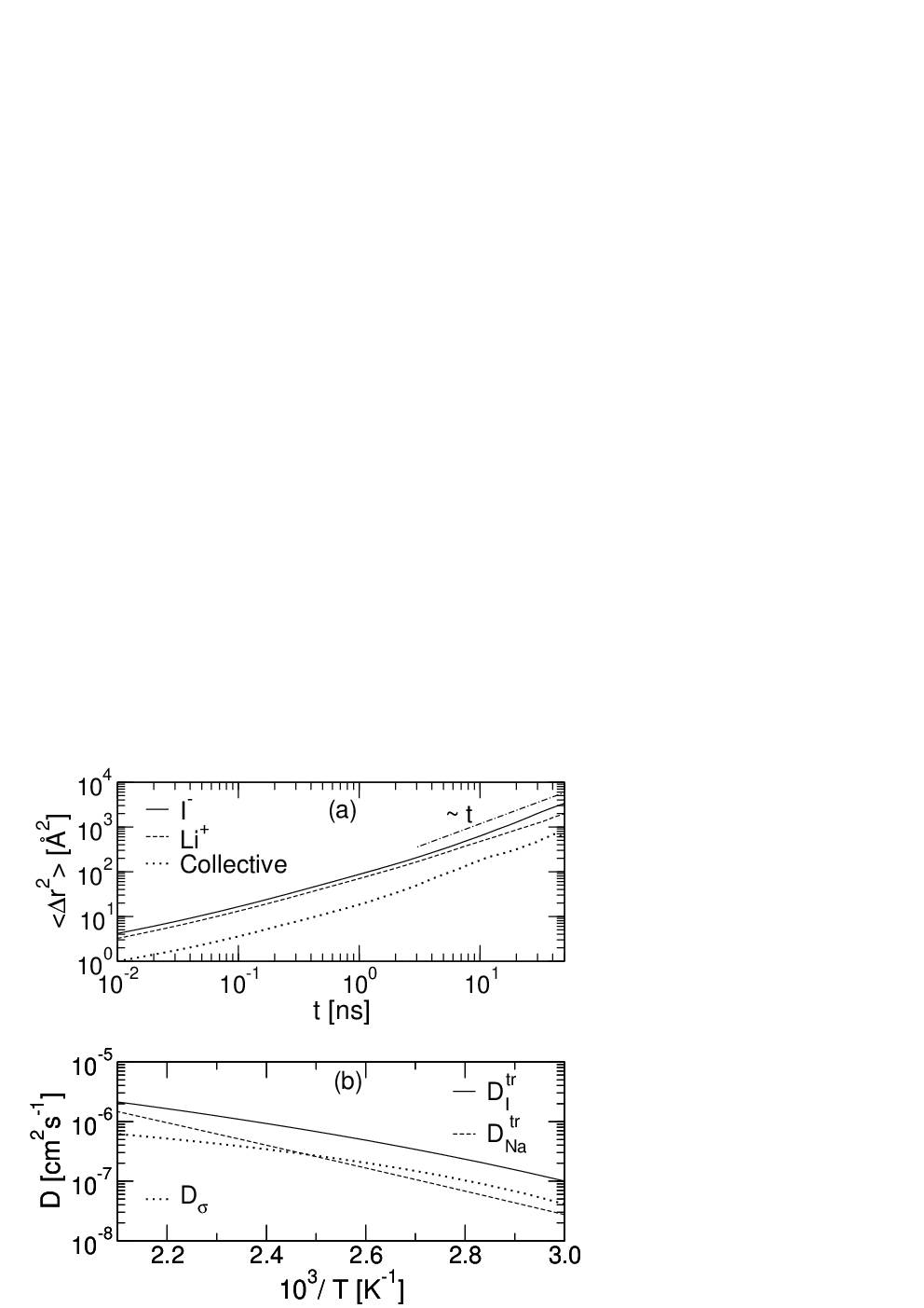
The mean square displacement (MSD) of Li+ and I- ions obtained from the MD simulation at T = 450 K are displayed in Fig. 2(a). The I- ions are slightly more mobile (by a factor of ) compared to the Li+ ions. The collective diplacement of the ions [see Eq. (2)] which measures the mean square displacement of the center of charge of the system is also shown in Fig. 2(a). The collective diffusivity, is diminished by a factor of approximately 3 with respect to the average diffusivity of the ions, . Fig. 2(b) shows the experimental values of the tracer diffusivities of Na+ () and I- () in PEO/NaI (EO:Na=30:1 and polymer chain lengths were of the order of ) from Ref. [16] as a function of temperature. The collective diffusivity for this system was reckoned from dc conductivity using Eq. (1). At T = 450 K factors of and are observed for the experimental system similar to the simulated PEO/LiI system. The absolute values of the diffusivities of the ions in the simulated and the experimental system are of the same order of magnitude at the considered temperatures. Furthermore, the reduction of the ionic diffusivity [i.e. ] is close to the experimentally observed value.
From the simulation we identify a non-free ion as one which is associated with a counterion such that it is separated by a distance of less than 4.6 Å that demarcates the first minimum of the Li I radial distribution function, [see Fig. 5 row 1, column 2]. Depending upon the number (one or two) of I- ions in the nearest neighbor shell of a Li+ ion one may speak of an ion-pair or an ion-triplet, respectively. The same cut-off radius is applied for defining a free or non-free I-. With this criterion the proportions of free and non-free ions present in the simulated system are displayed in Tab. 1.
| 0 | 1 | 2 | 3 | |
|---|---|---|---|---|
| Li [I]n | 6.2 | 75.9 | 17.9 | 0 |
| I [Li]n | 9.3 | 69.8 | 20.6 | 0.3 |

We have computed the MSD of a subset of Li+ or I- ions which are either free or participating in an ion-pair or ion-triplet (see Fig. 3). An ion was considered free during time if it had no counterion within its nearest neighbor distance for at least of the time . Also shown are the MSD of those Li+ ions which were paired with only one I- (but not necessarily with the same I-) for of the time. A similar definition was used for calculating the MSD of Li+ possessing two I- neighbors (i.e. ion-triplets). This definition limits the maximum values for because of the finite life-time [see Ref. [11]] of a specific local structure. The typical life-times of ion-pairs will be discussed in more detail further below.
It is observed that the dynamics of the free Li+ ions are almost indistinguishable from the paired Li+ ions in dramatic contrast to the result of the data fitting, reported in [16]. The present result is expected since most of the Li+ ions in the simulated system are coordinated to three to six contiguous ether oxygen atoms of the PEO backbone and all cations are found to be complexed by EO atoms. Thus, the Li+ dynamics mainly reflects the dynamics of the polymer chain. In particular, this strongly correlates the dynamics of free Li+ ions and paired Li+ ions. The dynamics of the subset of free I- are faster than the free Li+ ions by a factor of 1.6. The MSD of Li+ ions in the triplets are marginally slower compared to the Li+ in the pairs (Fig. 3). The I- in the ion-pairs are faster than the Li+ in the ion-pairs for short times ( ns) and beyond this merge together. The difference at short times reflects the restriction of Li+ motion due to the strong coupling to the polymer.
Even though the typical life-time of a Li I association only lasts for about
700 ps [11], there exist forward and backward jumps of the ions leading to an extension of the time duration that an ion is complexed to the same counterion. To see this clearly, Fig. 4 shows the probability that a particular pair of Li+ and I- separated by less than 4 Å exists at times and where is some reference time. On an average about 6 ns is required for a Li+ ion to change its I- neighborhood.
Over this timescale a Li+ ion translates along a polymer chain by a distance of approximately 4 monomers. Thus, the Li+ I- pairs move collectively along a chain. This is seen from Fig. 4 (inset) where the mean square variation of the ether oxygen index experienced by a Li+ while being still constrained to the same chain is plotted in time (also see Ref. [22]).

IV Ionic Correlations
The collective diffusivity can be calculated from the microscopic dynamics of the ions via
| (2a) | ||||
| (2b) | ||||
| (2c) | ||||
where is the displacement of a specific ion carrying a charge of during time . Whereas the self terms [i.e. the first term of Eq. (2b)] express the diffusivities of all ions (i.e. ), the cross terms contain the correlation effects between distinct ions and give rise to a non-trivial Haven ratio.

The second term of Eq. (2c) can be rewritten in terms of its different pair contributions. Using and one obtains
| (3) |
where
| (4) |
Here, denotes a set of cations or anions and the condition in the second summation of Eq. (4) implies that only distinct pairs of ions are considered. The negative sign in the middle term of the rhs of Eq. (3) results from the opposite signs of the charges on Li+ and I- ions. One expects in analogy to inorganic ion conductors a positive correlation of all ionic species, i.e. . However, since the correlation between Li+ and I- ions will turn out to be particularly pronounced, for a polymer electrolyte, one gets and in contrast to inorganic ion conductors where one only has the contribution of cation-cation pairs.
Our goal is to elucidate the origin of the correlations, contributing to . For this purpose we rewrite
| (5) |
where denotes the displacement vector of ion from its initial position at time to its final position at and refers to the unit vector of the displacement during time of ion starting from its initial location at . Thus, a necessary condition for a non-zero is the presence of directional correlations as expressed by the scalar product of the respective unit vectors. Qualitatively, one would expect that they mainly emerge from nearest-neighbor ions. Furthermore, the absolute value of might further increase, if nearby pairs are particularly mobile.
To quantify these different contributions to we introduce the following correlation functions between two distinct ions and
| (6a) | ||||
| (6b) | ||||
The function represents the directional correlation of two ions whereas reflects their joint mobility during times and .
In a first step these functions will be averaged over pairs of ions separated by distance . In general, the distance between two ions will change with time. A convenient way to take this into account is to use the initial and final inter-ionic separation distance with equal weight for the identification of . With an additional average over and using the abbrevation one can therefore define
| (7a) | ||||
| (7b) | ||||
where denotes the average over the time origins; is the normalization constant [proportional to ] and is the Kronecker delta function which bins the quantities and at both the initial and final distance between ions and . Next, averaging the functions over all distinct pairs of ions, we define
| (8a) | ||||
| (8b) | ||||
In the last step one can average over all distances. This yields
| (9) |
where we have defined
| (10) |
and is the number density of the ions (cations plus anions). The prefactor in Eq. (9) takes into account that the total number of unlike pairs () is twice the number of like () pair of ions . In Eq. (10) the number density per species is expressed as and the radial distribution function (rdf) for the pair of species is referred to as .
Likewise, one can define the quantity using relationships similar to Eq. (7) and (8). Our goal is to express (see Eq. 4) in terms of more elementary contributions. Based on the definitions, introduced so far, we can now write
| (11) |
which implicitly defines the function . If the directional correlation [via ] and the mobility correlation [via ] of a pair of ions are statistically uncorrelated then one has , i.e. . Possible correlations can be taken into account by slightly different values of . Fig. 5 depicts the functions , , and for the different pairs of ionic species []. The correlation functions, and are evaluated at specific times = 0.1 ns, 1 ns and 4 ns. One can see that is larger than one. The resulting correlation between the directional and the mobility correlation, however, is rather weak.
The high proportion of ion-pairs (Li I) present in the system manifests as a pronounced nearest neighbor peak in the at Å. In contrast, the rdfs between the like charges, and are of similar strength in their respective first and second nearest neighborhood but exhibit weaker local density when compared to . To quantify this effect we introduce
| (12) |
as the number of particles of species in the -th neighborhood of a particles of species (Note that the coordination numbers of around and around , in the different shells, are the same, considering equimolar amounts of either ionic species). Here, and are the minima of corresponding to the -th neighborhood. The values for for are listed in Tab. 2.
| L M | |||
|---|---|---|---|
| Li Li | 0.4 | 3.8 | 5.5 |
| Li I | 1.1 | 1.9 | 3.7 |
| I I | 0.3 | 3.3 | 5.2 |
In case that the system would have only free ions and well-defined Li I pairs the quantity would be identical to the fraction of non-free ions. However, about 20 % of all ions form ion-triplets. This increases the value of with respect to . Numerical analysis shows (see Tab. 1) which is, indeed somewhat smaller than . The presence of these triplets also provides one important contribution to and and thus to and . Due to the smallness of and one already anticipates that the contributions to from the like pairs is minor.
The joint mobility functions, i.e. the average of the product of the length of the displacement vectors of two distinct ions during time , , are plotted in the third row of Fig. 5 for the species Li Li, Li I and I I. We see, that this function is essentially independent of for all times and is very similar for all the three types of pairs. In agreement with Fig. 3 this means that spatial proximity of two ions does not enhance its mobility.
In contrast, decreases with for all types of pairs. Qualitatively, this is due to the screening of the interactions between the ions. Also, as time progresses becomes smaller for fixed . This is expected because each ionic aggregate has a finite lifetime beyond which it disintegrates. Each of the ions which were once part of an ionic cluster will, beyond a certain time, dislodge, migrate and finally participitate in the formation of another new cluster. We would like to mention that an ionic positional correlation function similar in spirit has been reported by Müller-Plathe et al [8, 7].
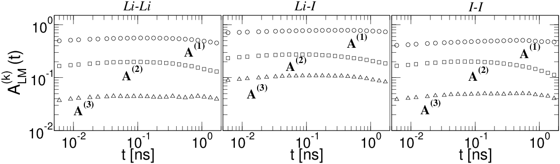
Among the general features of one can see that they decay with in a step-like manner. The steps, representing constancy in the correlation strength, are short spanned and located at pair separation distances corresponding to the peak positions of the . Thus, it may seem reasonable to characterize the average properties of the in the individual shells. For this purpose we define
| (13) |
where and are the minima of corresponding to the -th neighborhood (see Fig. 5). Analogously one can define and . In the following we analyze the first three shells . Their time dependence is shown in Fig. 6. The functions are more or less constant at short times. However, these curves display a trend of decay with increasing time, as expected. Correlations for all pairs of ionic species show the order: where . Henceforth, we will often refer to a timescale ns. Note that is significantly smaller than the typical life-time of a Li I pair. For we have , and . Thus, the directional strength of motion of a pair of unlike charges (Li I) is more potent in comparison to those of the like charges and is close to a perfect correlation . Furthermore, the shell-dependence is due to the screening of the higher shells of ions with respect to the central ion.
After having discussed the individual contributions to we now come back to Eq. (4) by rewriting it as
| (14) |
The correlations originating from the -th neighborhood
is contained in the quantity
.
From the previous discussion we have seen that the dependence of
on the ionic pair L M is mainly governed by
which for Li I is approximately 60 % larger
than for the like pairs. Since, also, is much larger
for Li I (see Tab. 2) the by-far dominant contribution
to stems from .
V Stolwijk-Obeidi Model

In this section we begin with exact microscopic expressions and proceed through steps of simplifications to construct an exact model similar in spirit to the phenomenological Stolwijk-Obeidi (SO) model. The specific procedure is determined by the input from simulations. The key idea of the SO model is to express the observed single-particles diffusivities, obtained via tracer diffusion, and the conductivity in terms of the properties of single ions and ion-pairs. In the SO model no triplets are taken into account. In case that these aggregates exist one should therefore better speak in terms of free ions or non-free ions, the latter possessing one or more counterion(s) in their coordination sphere, i.e. existing as both ion-pairs and ion-triplets in our case. In any event, this terminology gives rise to a more general applicability of that approach.
First, we start to derive the single-particle dynamics. Here we have to take into account that during the life-time of a pair the MSD does not reach the linear regime. This requires a definition for the long time behavior of the transient ionic states. Specifically, we define the MSD associated with ions of type (i.e. either Li+ or I-) existing in state [i.e. either free () or non-free ()] in the following manner:
| (15) |
Here stands for the instantaneous state of the ion , refers to the square of the displacement experienced by ion between times and and the Kronecker delta function picks the instantaneous state of ion at time . For smaller than the typical timescale of the lifetime of nonfree ions this definition would give rise to the data in Fig. 3. For , and start to merge because of averaging effects, i.e. free ions becoming non-free and vice versa.
The fraction of free or non-free ions can be written as
| (16) |
Using this somewhat complex but generic definition one can show that Eq. (15) and (16) can be combined (see Appendix) to yield
| (17) |
Note that the motion of state specific MSD is only given for times smaller than the average lifetime of a pair of ions LiI and thus in particular we choose .
The average dynamics of a non-free ion is characterised by
| (18) |
This definition can be used to relate the decrease in average ionic diffusivity to the correlated motion of the ions. Eq. (3) can be rewritten via the following steps at a chosen timescale t⋆:
| (19a) | |||||
| [cf. Eq. (14)] | (19b) | ||||
| (19c) | |||||
| (19d) | |||||
| [cf. Eq. (18)] | (19e) | ||||
| (19f) | |||||
In the last step we have defined
| (20) |
The parameters , and are the dimensionless correction factors required at every step of simplification in Eq. (19). captures the cross correlations between the like charges. Because the missing contributions to have opposite sign one naturally has . accounts for ignoring correlations between Li+ and I- ions beyond the nearest neighborhood ( Å). One has because of the presence of anticorrelations between the pair of ions beyond Å. The origin of the anticorrelations is not yet comprehended fully, however, physically this might arise from the tendency of the subensemble of particles to nullify its momentum due to a finite simulation box size. is the correction due to the -factor [see Eq. (11)], which is given by the average value of in the nearest neighbor shell, reflecting correlations between the directional and the mobility correlations. expresses the non-ideality of directional correlation in the nearest-neighbor shell, i.e. . The factor is needed to approximate by . If one compares the quantities and the latter is either greater than or equal to the former. This rationalizes . Lastly in the final step the factor is required which as discussed above is larger than one. The individual values of for are listed in Tab. 3.
| 0.959 | 1.221 | 0.966 | 0.94 | 0.88 | 1.1 | 0.86 | 0.92 | 1.18 | 1.07 | 0.82 |
Next we define the following parameters for later convenience:
| (21) |
The time dependence of the parameters , and is shown in Fig. 7. These are observed to be roughly stationary within the 1 ns time window which is less than the maximum life-time of an ion-pair. The values measured at ns for the present system at T = 450 K can be found in Tab. 3. We have verified that choosing ns instead for defining the parameters would virtually yield similar magnitudes of results that are presented later.
That the value of ) is less than unity (0.96 and 0.91 for T = 450 K and 425 K respectively), can be understood from the slightly slower dynamics of the ion triplets than the free and the paired ions. It must be noted that is a consequence of the coupling between ion and segmental dynamics of PEO. On the other hand means that the I- ions in the pairs are slightly faster than their Li+ counterparts at short timescales (see also Fig. 3). It is interesting that the correction factor is found to be less than unity (see Fig. 7) unlike the assumption of in the SO model. In essence, all the fixed parameters (, , and ) are close to unity due to the natural outcome of the ionic association and dynamics in the system and which is why the SO model could approximately define these characteristics. All these parameters are found to be nearly the same when going from the temperature of 450 K to 425 K (not shown). Even though differs slightly between the temperatures, the final product is found out to be similar due to compensation of the increase of one factor by the decrease of another factor and vice versa.
The diffusion constant can be written as . Furthermore, we define
| (22) |
through which we are extrapolating the short time dynamics of the transient ionic state of species to long times using the time dependence of as a reference. This extrapolation is necessary because is only defined for times of the order of the lifetime of the ion in state which is smaller than the timescale over which the ions become completely diffusive. As a specific advantage of the definition of , Eq. (17) can now be rewritten as
| (23) |
which is the form used in the SO model with .
In the SO model all are assumed to be one. According to the above discussion this corresponds to the case of ideal Li I pairs and no directional correlations for other pairs (either pairs of like ions or pairs of Li+ and I- ions beyond the nearest neighbor shell). Multiplying Eq. (19f) with the factor and using one obtains from Eq. (19f) and (18)
| (24) |
Here, is the product of the parameters . We have introduced the parameters and which are required for an exact relation between the diffusion coefficients in Eq. (24) and are defined as and with
| (25) |
This parameter (see inset of Fig. 7) captures the difference in timescales over which and approach the linear regime, i.e. the respective ionic dynamics become diffusive. In the present case one has and by choosing ns at T = 450 K (see Fig. 7). means that Li+ becomes diffusive later than I- ions which is evident from Fig. 2(a). As discussed in Ref. [22] the diffusive behavior of the Li+ ions for long chains is achieved via jumps between different PEO chains. The residence time of the cation with one chain is found to be 100 ns [22]. Only for short chains (as in the present case) the timescale of Li+ diffusion will be somewhat shorter because of the dominance of the center of mass diffusion of the polymer. In contrast, an I- ion change its cationic neighbor(s) quite frequently over a timescale of 7 ns and therefore is able to become diffusive faster than its cationic counterparts.
In the following, we formally define , , . The set of three equations, [Eq. (23) with and Eq. (24)] is identical to the SO model if , , and i.e. if the picture of strict Li I pairs would hold. However, these three equations contain four parameters (, , , ). Due to this ambiguity there are many possible solutions for a given set of parameters. The solution, presented in Ref. [16] involved additional assumptions about a similar temperature dependence of the parameters. The resulting solution was for high temperatures. To circumvent this problem we have introduced the dimensionless parameter as in Eq. (21) and determined its value (similar to , , ) from simulations. The reason for the observed magnitude of has been explained above.
Using these parameters the relations of the generalized SO-model (see also Appendix II) can be solved:
| (26a) | |||
| (26b) | |||
| (26c) | |||
The quantities , and are experimentally accessible. The parameters , , , , and can be gathered from simulations, thereby permitting a solution for the unknowns , and from Eq. (26). We neglect the possible temperature dependence of , , , and because it is difficult to find a priori arguments to estimate the temperature dependence of the four parameters.
VI Application of Stolwijk-Obeidi Model
First, we aply the SO model to our simulation data. We employ the parameters of Tab. 3 and cm2s-1, cm2s-1 and cm2s-1 (obtained through Fig. 2(a) from the simulation at T = 450 K) that gives cm2s-1. These when plugged into Eq. (26) yields the following: , cm2s-1 and cm2s-1 and thus . From Eq. (25) one should then obtain . These, when compared to the actual values culled directly from the simulation, e.g., (see Tab. 1) and (from Fig. 3) are reproduced, in good agreement with the solutions of Eq. (26). By letting and the other parameters of Tab. 3 unchanged one obtains and from Eq. (26). Clearly, the factors and are important.
Next, we apply the model on the same representative PEO/NaI polymer electrolyte with the concentration of EO:Na+ = 30:1 as Stolwijk and Obeidi did. Accordingly, we use the tracer diffusivities of Na+ () and I- () and the collective diffusivity () from Ref. [16] at different temperatures as input. Note the experimental data that have been used subsequently in this work is calculated back analytically from the fit results of Ref. [16] using the VTF temperature dependence of the single ion diffusivity prefactors and the Arrhenius temperature dependence of the pair formation constant (see details in Ref. [16]). Four different sets for the parameters , , , , and are considered which we will refer, henceforth, as SET I to SET IV and tabulated in Tab. 4. This will allow delineation of the relative importance of the parameters.
| SET | ||||||
|---|---|---|---|---|---|---|
| SET I | 0.959 | 1.221 | 0.966 | 0.848 | 1.065 | 0.818 |
| SET II | 0.959 | 1.221 | 0.966 | 0.848 | 1.0 | 1.0 |
| SET III | 0.959 | 1.0 | 1.0 | 1.0 | 1.0 | 1.0 |
| SET IV | 74 | 1.0 | 1.0 | 1.0 | 1.0 | 1.0 |
SET I has been retrieved from our simulation (same as in Tab. 3) and additionally, we assume this to be similar to the case of Na+ ion in PEO. SET IV corresponds to the original SO model of Ref. [16]. Furthermore, we have superimposed a weak noise having a strength between to the experimental data [i.e , and ] in order to evoke an impression about the stability of the solution (, and ). The mean and standard deviation of the unknowns are calculated for each temperature from 100 independently noised realisations. We had also attempted mixing noise to the experimental data, however, the standard deviations of the solution exceeded mean values in the high temperature limit. Thus, the accuracy of the input experimental data is imperative in deriving the estimates of the solutions.


Fig. 8(a) shows the values of diffusivities of the free Na+ (dotted line) and free I- (solid line) obtained from the solution of Eq. (26) with the parameters SET I. It can be observed that is larger than over the temperature range shown. The curves monotonically decrease from the high to the low temperature end. exceeds by about a factor of about 67 at the low temperature end to about 23.5 at the high temperature end. Particularly, at T = 450 K, which is about a factor of 1.8 larger than what is seen in the simulation (i.e. ). However, this factor is expected to depend upon the chain length of the polymer host as shown in Ref. [20] in agreement with the current observations. By only supplanting the parameters in SET I and letting the others unaltered (i.e. SET II) one observes a strong shift by a factor of 3 in (dashed line) to larger values especially at the high temperatures and by about 20 % at the low temperatures. By choosing the parameters from SET III, decreases less than 20 % at high temperatures and even less at low temperatures [see Fig. 8(b)] when compared against SET II. Choosing the values and (i.e. SET IV) would have reproduced the results obtained by Stolwijk-Obeidi (not shown) at all temperatures.
The dynamics of the free Na+ ions exhibits insignificant alteration between the parameter sets I, II and III. This can be explained from Eq. (26)(b) under the condition which gives and therefore making relatively independent of the parameters.
In the foregoing, we have identified and as important players in the estimation of while applying the extended SO model to our simulation data. Provided that , as is the case for the polymer electrolyte under investigation, a change in the other parameters (, and ) are not as important in generating the large change in the diffusivity of the free I- ions at the high temperatures. We, next, show that the reason for the large sensitivity of originates primarily from the small changes in whereas the influence of in this case is rather weak. If then (from Eq. (29) and Eq. (26)(a)) and (see Appendix II) which implies that . From Eq. (23), , and if is large then the second term in the numerator of the rhs dominates and the denominator is also correspondingly small. Therefore, a small decrease in can cause a large increase in as observed in Fig. 8(a) at high temperatures where the fraction of non-free ions is large (see below). In contrast, at lower temperatures the proportion of non-free I- ions drops and thereby stabilizing from small variations in .
Fig. 9(a) shows the corresponding fraction of non-free ions for the sets I, II and III. Similar to the plots of diffusivities of the free ions, one finds monotonously decreasing and lightly bent behavior over the entire temperature range. Moving from SET I to SET II one observes an increase of by about 6 % which can be explained from the proportionality: . In contrast, while changing parameters from SET I to SET III there is only a inconspicuous increase in the proportion of non-free ions by less than 2 %. This is due to the nullifying effect of the simultaneous variation of the parameters between the two sets of parameters and thus, appearing as similar fractions of non-free ions which is rather a mere coincidence. Choosing SET IV, however, results in a scanty fraction of non-free ions (see Fig. 9(b)).

Finally, the ion-pairing reaction constant, [see Ref. [16, 30]] for the equilibrium reaction Na+ + I- Na+I- at the different temperatures is analyzed. Note that the above equation of is strictly applicable only if the non-free ions exist as ion-pairs. These are shown in Fig. 10 for the four cases mentioned.
For the original SO model (SET IV) the values are orders of magnitude less than those obtained
from the other sets primarily due to the parameter.
A fit with where is the prefactor,
is the formation energy of the pair and is the Boltzmann constant yields the energetic term. This is listed in Tab. 5 along with the fraction of non-free ions at T = 450 K compiled for the different cases and sources.
calculated from the simulation using at T = 450 K is consistent with that obtained from the experiment by using the extended SO model with the parameters in SET I. Comparing the fraction of non-free ions between the original SO model [16] () against the extended SO model with SET I () the discrepancy is evident at T = 450 K. In fact for the former a high ion-pair diffusivity is required to match the small fraction of ion-pairs in order to generate a reduction of the average ionic diffusivity by a factor of 3 to be compatible with the observed collective diffusivity. Note that with SET II (i.e. by neglecting the importance of ) one would have been tempted to erroneously conclude that the pair formation is not governed by a single . As an additional information, the pair formation energy determined from the Raman spectroscopic work on poly(propylene oxide)PPO/NaCF3SO3 with O:Na = 30:1 by Kakihana et al. [31] provides eV but with a high pair fraction. Of course, it would have made an interesting comparison if spectroscopic data had been available for the PEO/NaI system.
| System | Remark | [eV] | |
|---|---|---|---|
| (T = 450 K) | |||
| PEO/LiI (20:1) | Simulation | 0.31 | 0.92 |
| PEO/NaI (30:1) | Params, SET I | 0.33 | 0.88 |
| (Tab. 3) | |||
| PEO/NaI (30:1) | Ref. [30] | 0.19 | 0.08 |
| PPO/NaCF3SO3 (30:1) | Ref. [31] | 0.16 | 0.70 |
VII Summary
In the first section ionic correlations in a polymer electrolyte (e.g. the archetypal PEO/LiI) stemming from ionic associations are elucidated by constructing elementary correlation functions. One of these functions included the time-evolution of the directional correlation of a pair of ions (both like-charged and unlike-charged) in dependence of the separation distance between the ions. The correlations from the Li I pairs are found to be the strongest in comparison to the Li Li and I I pairs of ions. Furthermore, the correlation effects are found to exist beyond the nearest neighborhood of counterions, albeit reduced due to the screening of interactions. In essence, the strong structural correlations together with the non-trivial values of the directional correlations between the cation-anion pairs lead to a reduction of the ionic conductivity of the polymer electrolyte compared to the average diffusivity of the ions. The joint mobility of a pair of ions calculated as the product of the magnitude of the displacement vectors of the ions showed that during a certain time this is almost independent of the structural correlations between the ions. One can thus infer that the dynamics of the different states of ions (i.e. free ions, ion-pairs, ion-triplets etc.) will be similar. Intuitively, due to the fact that most of the lithium ions are coupled to the ether oxygen atoms of the PEO one would expect some correlations between the dynamics of the free and the associated ions. This is, additionally, verified by computing the mean square displacement of the free Li+, isolated LiI- pairs and the isolated ILiI- triplets. This is in stark contrast to the conclusion from the Stolwijk-Obeidi model [16] which predicted the dynamics of ion-pairs to be orders of magnitude faster than the free ions.
In the second section the SO model is extended by starting from the Einstein-like equation which describes the collective diffusivity of the ions from the single-particle dynamics of the ions (the self terms) and the correlations from the distinct pairs of ions. Instead of describing the overall correlation effects only in terms of the dynamics and the fraction of isolated ion-pairs we generalised the approach by considering the dynamics and the fraction of non-free ions. Typically, the non-free ions account for the presence of ion-triplets or any higher order clusters along with the ion-pairs. Additionally, various approximation parameters, , are incorporated that keep track of the simplifications made to the correlated term of the Einstein-like equation. The simplifications can further be understood in terms of simple microscopic pictures. The parameters could be extracted from simulations and are found to be close to unity which is a consequence of the nature of ionic association and dynamics in polymer electrolytes. If each of these parameters except (which appeared as a result in the SO model) are chosen to be exactly unity one recovers the SO model. The extended SO model along with the inference of dynamical similarity between the free and the non-free ions is applied to the same data as in Ref. [16] but with the additional parameters chosen from simulation.
It is found that the fraction of non-free ions are high and consistent with the simulation results. The parameter also turns out to be more important compared to the other parameters (, , , ) specifically for yielding the estimates of the diffusivity of free I- ions. Typically, expresses the difference in timescales over which the cations and the anions become diffusive and reflects a characteristic of polymer electrolytes where the cations are predominantly complexed with atoms/groups located along the main backbone of the polymer for larger timescales in comparison to the anions which are coordinated to the same cationic neighbors for relatively short times. It must be, however, borne in mind that the results (i.e. fraction of non-free ions and the diffusivity of free ions) from the SO model depend on the accuracy of the input experimental data and possibly on the temperature dependence of one or more of the parameters (e.g. , ).
Further work is required to map the values of the parameters as a function of interaction between ions and the resulting collective diffusivity of ions that would impart general applicability to quantifying ionic association.
Appendix I
Let be the total number of ions in the system and so the number of cations and anions are respectively. Defining the quantity as follows
| (27) |
one can show that Eq. (17) can be derived from Eq. (15) and Eq. (16) through the following steps:
| (28a) | ||||
| (28b) | ||||
| (28c) | ||||
| (28d) | ||||
| (28e) | ||||
Appendix II
Here, we show how to rewrite Eq. (23) (for and ) and Eq. (24).
The fraction of non-free Li+ ions can be determined as : . Therefore,
| (29) |
The corresponding proportion of free Li+ and I- ions are given by and . The solutions given in Eq. (26) can be obtained from the following equations:
| (30a) | ||||
| (30b) | ||||
| (30c) | ||||
where we have used Eq. (21) and specifically
in Eq. (30a) we have used . Straightforward manipulation then gives rise to Eq. (26)(a-c).
Acknowledgement
We thank M. Schönhoff, N. A. Stolwijk and M. Vogel for several helpful comments and discussion. This work is carried out within the framework of Sonderforschungsbereich 458 and supported by the NRW Graduate School of Chemistry, Münster.
References
- [1] M. A. Ratner, Polymer Electrolytes Review - 1 & 2 (Elsivier, London, 1987, 1989).
- [2] P. G. Bruce and C. A. Vincent, J. Chem. Soc. Faraday Trans. 89, 3187 (1993).
- [3] B. Scrosati and C. A. Vincent, MRS Bull. 25, 28 (2000).
- [4] M. A. Ratner, P. Johansson, and D. F. Shriver, MRS Bull. 25, 31 (2000).
- [5] M. P. Allen and D. J. Tildesley, Computer Simulation of Liquids (Clarendon, Oxford, 2004).
- [6] D. Frenkel and B. Smit, Understanding Molecular Simulation (Academic Press, 2002), 2nd ed.
- [7] F. Müller-Plathe and W. van Gunsteren, J. Chem. Phys. 103, 4745 (1995).
- [8] F. Müller-Plathe, Acta Polymer. 45, 259 (1994).
- [9] S. Neyertz and D. Brown, J. Chem. Phys. 104, 3797 (1996).
- [10] O. Borodin and G. D. Smith, Macromolecules 31, 8396 (1998).
- [11] O. Borodin and G. D. Smith, Macromolecules 33, 2273 (2000).
- [12] O. Borodin, G. D. Smith, and R. L. Jaffe, J. Comp. Chem. 22, 641 (2001).
- [13] O. Borodin, G. D. Smith, and R. Douglas, J. Phys. Chem. B 107, 6824 (2003).
- [14] O. Borodin and G. D. Smith, Macromolecules 39, 1620 (2006).
- [15] The collective diffusivity in the Ref. [16] have an additional factor of 2, i.e. where is the collective diffusivity defined in this article.
- [16] N. A. Stolwijk and S. Obeidi, Phys. Rev. Lett. 93, 125901 (2004).
- [17] S. Obeidi, N. A. Stolwijk, and S. J. Pas, Macromolecules 38, 10750 (2005).
- [18] S. J. Pas, R. D. Banhatti, and K. Funke, Solid State Ionics 177, 3135 (2006).
- [19] A. Y. Akgöl, C. Hofmann, Y. Karatas, C. Cramer, H. D. Wiemhöfer, and M. Schönhoff, J. Phys. Chem. B 111, 8532 (2007).
- [20] K. Hayamizu, E. Akiba, T. Bando, and Y. Aihara, J. Chem. Phys. 117, 5929 (2002a).
- [21] K. Hayamizu, K. Sugimoto, E. Akiba, Y. Aihara, T. Bando, and W. S. Price, J. Phys. Chem. B 106, 547 (2002b).
- [22] A. Maitra and A. Heuer, Phys. Rev. Lett. 98, 227802 (2007).
- [23] E. Lindahl, B. Hess, and D. van der Spoel, J. Mol. Mod. 7, 306 (2001).
- [24] S. Nosé, Molec. Phys. 52, 255 (1984).
- [25] W. G. Hoover, Phys. Rev. A 31, 1695 (1985).
- [26] M. Doi and S. Edwards, The Theory of Polymer Dynamics (Oxford Science Publications, 2003).
- [27] O. Borodin and G. D. Smith, J. Phys. Chem. B 107, 6801 (2003).
- [28] G. D. Smith, R. L. Jaffe, and H. Partridge, J. Phys. Chem. A 101, 1705 (1997).
- [29] The interactions involving the I- in Tab. 4 and 6 of ref. [28] were modified as follows: kcal/mol, Å-1, ; Å6 kcal/mol , . All parameters were scaled by a factor of 0.71. Additionally, the equation of the force involving the term was scaled by a distance dependent scaling factor beyond 3.6 Å () with . The force fields were then reasonably fitted with Buckingham potential in the present work.
- [30] N. A. Stolwijk, M. Wiencierz, and S. Obeidi, Faraday Discuss. 134, 157 (2007).
- [31] M. Kakihana, S. Schantz, and L. M. Torell, J. Chem. Phys. 92, 6271 (1990).