Near-Maximal Mixing of Scalar Gluonium and Quark Mesons: A Gaussian Sum-Rule Analysis
Abstract
Gaussian QCD sum-rules are ideally suited to the study of mixed states of gluonium (glueballs) and quark () mesons because of their capability to resolve widely-separated states of comparable strength. The analysis of the Gaussian QCD sum-rules (GSRs) for all possible two-point correlation functions of gluonic and non-strange () quark scalar () currents is discussed. For the non-diagonal sum-rule of gluonic and currents we show that perturbative and gluon condensate contributions are chirally suppressed compared to non-perturbative effects of the quark condensate, mixed condensate, and instantons, implying that the mixing of quark mesons and gluonium is of non-perturbative origin. The independent predictions of the masses and relative coupling strengths from the non-diagonal and the two diagonal GSRs are remarkably consistent with a scenario of two states with masses of approximately and that couple to significant mixtures of quark and gluonic currents. The mixing is nearly maximal with the heavier mixed state having a slightly larger coupling to gluonic currents than the lighter state.
1 Introduction
The interpretation of the nature of the lightest scalar mesons is one of the most fascinating problems in hadronic physics. The plethora of scalar () states below [1] cannot be described by a simple nonet, a situation indicative of exotic states such as gluonium (glueballs) or multi-quark () states amongst the known scalar mesons. In the gluonium scenario, two-body decays to pseudoscalars suggest that the , and contain strong mixtures of gluonium and mesons [2], with the favoured as the dominant glueball state [3]. Analyses based on chiral Lagrangians [4, 5] suggest that the and are mainly gluonium states with a small gluonium component of the [4]. Other phenomenological approaches present a scenario of mixing between a glueball and the , states of a nonet [6]. Lattice QCD calculations lead to a scalar gluonium state of approximately with quenched quarks [7]. However, with dynamical quarks the mixing with states appears to be very strong, driving the mass of the lightest flavour-singlet meson down toward with tentative identification of an excited state on the order of [8]. The vast literature on mixing of gluonia in QCD sum-rules is reviewed in detail in [9]. The key findings of QCD Laplace sum-rules are that admixtures of scalar gluonium and () states exist with masses of approximately and [9, 10, 11, 12], a conclusion that is also upheld by studies based on Gaussian QCD sum-rules [13, 14, 15]. In particular, the mixing that results from QCD sum-rules is very large [9, 10], with comparable couplings of these states to gluonic and currents [13, 14, 15].
The results of these different approaches suggest that a consistent scenario of -gluonium mixing is manifested in the scalar hadronic spectrum as two states on the order of and that couple to a significant mixture of and gluonium currents. From both the QCD sum-rule and lattice perspectives, this implies that the non-diagonal correlation function between and gluonic currents must be large enough to describe this behaviour. However, perturbative contributions to the non-diagonal correlation function (and hence mixing between gluonium and quark mesons) are chirally suppressed [16, 17, 18, 19]. Non-diagonal correlation functions have been analyzed in detail for pseudoscalar gluonium leading to a small mixing angle even in the presence of chiral-violating condensates [16]; given the similarities in field-theoretical structure between the scalar and pseudoscalar channels, a similarly small mixing angle in the scalar channel seems unavoidable [16, 19]. However, the mixed condensate effects, which are zero at leading order in the pseudoscalar channel [16], are shown below to be non-zero for the scalar channel providing a scale for large mixing. In addition, we consider instanton effects in our analysis; such effects have been argued to be essential for studies of gluonium [20]. As will be seen below (and as argued in [21] for glueball decays), the full inclusion of chiral-violating effects of QCD condensates and instantons provide the dominant contributions to the non-diagonal correlator in the scalar channel. These chiral-violating effects in the non-diagonal correlator are essential for a self-consistent scenario of two states coupling to a strong (near maximal) mixture of gluonium and currents; this scenario emerges from all possible correlation functions of gluonic and quark currents (i.e., diagonal gluonic, diagonal , non-diagonal gluonic-).
The formulation and analysis of Gaussian sum-rules is reviewed in Section 2. In Section 3 the leading-order perturbative, QCD condensate, and instanton contributions to the non-diagonal correlation function of and gluonic currents are calculated along with the associated Gaussian QCD sum-rules. The analysis of the Gaussian sum-rules and the pattern of state coupling mixing is then presented in Section 4.
2 Review of Gaussian Sum-Rules
Gaussian sum-rules associated with QCD two-point correlation functions have been shown to be sensitive to the hadronic spectral functions over a broad energy range, and analysis techniques have been developed to exploit this dependence to determine how resonance strength is distributed in the spectral function [13, 14, 15]. Thus Gaussian sum-rules are well-suited to situations such as -gluonium mixing where multiple hadronic states could contribute to a correlation function.
The () Gaussian sum-rule (GSR), introduced in [22], is given by
| (1) |
and relates a QCD calculation to a weighted integral of its associated hadronic spectral function from its threshold . The Gaussian kernel peaked at smears the spectral function through an (approximate) interval . This smearing provides a clear conceptual implementation of quark-hadron duality. The width of this duality interval is constrained from below by QCD because renormalization-group improvement of sets the renormalization scale through [14, 22]; therefore it is not possible to achieve the formal limit where complete knowledge of the spectral function could be obtained through
| (2) |
In contrast, the variable in (1) is unconstrained by QCD and can be varied to probe excited and ground states with similar sensitivity. Any features of the spectral function strong enough to be isolated from the continuum will be revealed through the GSR. This behaviour should be compared to that of the Laplace sum-rules
| (3) |
which exponentially suppress excited states relative to the ground state.11 1 The configuration-space correlation function in (4) as used in lattice QCD involves exponential suppression of excited states similar to that occurring for Laplace sum-rules.
Sum-rules analyses start from the calculation of an appropriate QCD correlation function of renormalized composite operators. We focus on two-point functions of scalar operators and
| (4) |
where and can be the same (diagonal) or different (non-diagonal). The correlator (4) is related to a hadronic spectral function through a dispersion relation with a number of subtraction constants. For example, in the diagonal scalar gluonic case, we have
| (5) |
Unknown subtraction constants and field-theoretical divergences can be eliminated by constructing the GSRs22 2 This definition is a natural generalization of that given in [22]. To recover the original GSR, we simply let in (6).
| (6) |
where and where the Borel transform is defined by
| (7) |
Applying (6) to (5) yields the following one-parameter family of GSRs (see [13] for further details):
| (8) |
Note that the sum-rule can only be used in situations where there exists an appropriate low-energy theorem from which we can determine the subtraction constant . Such is the case, for instance, with the diagonal scalar gluonic two-point function [18].
On the right-hand side of (8), we impose a fairly general resonance(s) plus continuum model
| (9) |
where represents the onset of the QCD continuum. The resulting continuum contribution
| (10) |
is then moved to the left-hand side of (8). The total QCD contribution
| (11) |
then satisfies
| (12) |
Integrating both sides of (12) with respect to gives
| (13) |
in which the right-hand side is recognized as the member of the finite-energy sum-rule (FESR) family. Thus, the information contained in the GSRs which is independent of the FESRs can be isolated by considering the normalized Gaussian sum-rules (NGSRs) [14]
| (14) | |||
| (15) |
which are related to the hadronic spectral function via
| (16) |
For diagonal correlation functions the spectral function obeys a positivity constraint so the NGSR must exist. For non-diagonal correlators the possibility of state mixing implies that could change sign, so it is possible that either or the denominator on the right-hand sides of (14) or (16) could be zero. In such situations, the GSRs would have to be analyzed instead of the NGSRs.
We next consider the currents that will be used to probe the gluonic and aspects of the scalar hadronic states. Refs. [10, 23] argue eloquently that the mixing of mesons and gluonium is unavoidable because of the trace anomaly for the energy-momentum tensor [24]
| (17) |
where
| (18) | |||
| (19) | |||
| (20) |
Equation (17) actually contains two multiplicatively-renormalizable (renormalization-group invariant) composite operators: and . From a strictly field theoretical perspective, both are suitable choices for currents. However, the gluonic and/or nature of states which couple to the current would be difficult to disentangle. As such, we instead follow [16] and use renormalized currents
| (21) | |||
| (22) |
where denotes a renormalized composite operator and denotes bare quantities. Our convention for dimensional regularization uses spacetime dimensions. Of course the form of the renormalized operator (21) necessarily underlies the renormalization-group invariance of the trace anomaly (17) (see e.g. [25]). However, the advantage of the current is that its tree-level expansion is purely gluonic allowing a qualitative separation of gluonic and degrees of freedom. Note that the use of a scalar tri-gluonium current, with three factors of the field strength rather than two as in (21), does not seem to couple to the lightest state and mixes weakly [26]. The non-strange current has isospin and is renormalization-group invariant.
We define diagonal correlators corresponding to (21) and (22) as follows:
| (23) | |||
| (24) |
where . Although both correlation functions are probes of scalar mesons, those states which have a more significant overlap with the gluonic current should predominate in (23); those states which are dominantly of a non-strange quark () nature should be more significant in (24). A mixed state with substantial gluonic and quark components (i.e., a state that couples to both the gluonic and quark currents) should self-consistently appear in an analysis of both correlation functions. In particular, independent predictions of identical-mass states from QCD sum-rule analyses of both (23) and (24) would be indicative of mixing. Note that the currents are simply probes of the actual hadronic spectrum and do not impose a particular interpretation on the states: any state that has non-strange content would be probed by , and any state with gluonic content would be probed by regardless of any additional content (e.g., ) in the states.
In the scalar gluonic channel, a low-energy theorem (LET) [18]
| (25) |
allows construction of the GSR. The significance of instanton contributions in the overall consistency of the LET-sensitive sum-rule and the LET-insensitive sum-rules was first demonstrated for Laplace sum-rules [27, 28]. A similar consistency is observed for Gaussian sum-rules, but theoretical uncertainties are better controlled in the GSRs [13]; hence, we focus here on the GSRs for both the diagonal gluonic and quark channels. QCD expressions for the GSRs and corresponding to the diagonal correlation functions (23), (24) can be found in [13, 14].
3 Non-Diagonal Correlation Function and GSRs of and Gluonic Currents
The non-diagonal correlation function for quark and gluonic currents
| (26) |
contains perturbative, QCD condensate, and instanton contributions
| (27) |
The leading-order perturbative diagrams that contribute to are given in Fig. 1. The first diagram, a two-loop calculation, corresponds to the (bare) gluonic term in (21). The second, a one-loop calculation, corresponds to the (bare) quark term arising from composite-operator renormalization (i.e., it is a renormalization-induced diagram). Despite the differing number of loops, both diagrams are .33 3 Strange (and heavier) quarks originating from composite operator renormalization in (21) will be suppressed by an additional factor of . Also, both diagrams have the same leading chiral behaviour because the quark loop in the first diagram provides a chiral suppression factor. The perturbative contributions can thus be separated into these bare and renormalization-induced diagrams
| (28) |

At leading chiral order in the scheme, the result for (corresponding to the two-loop diagram in Fig. 1) is
| (29) |
where is the renormalization scale. We have ignored non-logarithmic terms in (29) as they correspond to dispersion relation subtraction constants which are eliminated upon forming the GSRs. The term in (29) is problematic since it cannot be renormalized away or absorbed into a dispersion-relation subtraction constant. However, the leading chiral order contribution arising from the one-loop renormalization-induced diagram of Fig. 1 is
| (30) |
where we have again ignored non-logarithmic terms. An important, but subtle, aspect in the calculation of is retaining order contributions from the loop integrals that lead to finite terms when combined with the renormalization constant appearing in (21). This methodology is necessary and can be verified for well-known correlation functions (e.g., light-quark pseudoscalar currents). The offending term in (29) is thus cancelled by a compensating term in (30), and we are left with the leading-order -scheme perturbative contribution to the non-diagonal correlation function:44 4 The numerical coefficients in this result disagree with those presented in Ref. [16], although the overall chiral and logarithmic dependence is identical. We have checked our calculational methodology by verifying the pseudoscalar results in [16] and believe that (32) is correct.
| (31) | |||
| (32) |
The QCD condensate contributions [30] to the non-diagonal correlator, including operators up to dimension-five, can be written as an operator-product expansion (OPE)
| (33) | |||
| (34) |
As will be shown below, the chiral violating effects of the quark condensate and mixed condensate will dominate that of the gluon condensate . To obtain the leading chiral order behaviour of the OPE coefficients, it is necessary to include higher-order mass contributions that result in operator mixing [31, 32]. In particular, the naively-calculated unmixed OPE coefficients , , and are related to the coefficients in (33) by [31]
| (35) | |||
| (36) |
In principle, the coefficient of the identity operator (i.e., perturbative contributions) also mix with the quark condensate coefficients, but such terms are proportional to and are therefore sub-leading in the quark mass compared with (32).
The quark condensate contribution to the non-diagonal correlator is easily calculated to leading chiral order using any of the equivalent methods for evaluating OPE coefficients [33]. As in the perturbative case, in principle there are two classes of diagrams, both of which are depicted in Fig. 2. However, the renormalization-induced diagram of Fig. 2 is chirally-suppressed relative to (37) and so represents subleading effects. Computing the first set of diagrams in Fig. 2 therefore gives the leading-order quark-condensate contributions
| (37) |

Figure 3 shows two of the diagrams that contribute to the mixed condensate OPE coefficient. Within fixed-point gauge methods, the two-quark vacuum expectation value appearing in the renormalization-induced diagram of Fig. 2 also introduces the mixed-condensate (see e.g., Ref. [34]). However, the two renormalization-induced diagrams are suppressed by a factor of and additional factors of the quark mass compared with the first diagram of Fig. 3, resulting in the following leading-order OPE coefficient
| (38) |

In the absence of operator mixing, the diagrams that could lead to the gluon condensate OPE coefficient are shown in Fig. 4. However, the renormalization-induced diagrams are higher-order in and hence are subleading. Because of infrared divergences, it is necessary to retain the quark mass until the last steps of the calculation and then extract the leading chiral behaviour. Using plane-wave methods with we find
| (39) |
where
| (40) | |||
| (41) | |||
| (42) |
The divergences in and cancel, leaving a finite result as required given the pre-factor. The logarithmic correction from is seen to be subleading compared with the logarithmic correction from . Thus the leading-chiral gluon condensate contribution to the non-diagonal unmixed OPE coefficient is
| (43) |
The infrared divergence in (43) is now cancelled when (43) and (38) are substituted in (36), resulting in the leading-order contribution to the gluon condensate OPE coefficient
| (44) |
The cancellation of the infrared divergence follows from the methodology of [31], and provides a consistency check on our calculation of the OPE coefficients.

Finally, the result of our calculation for the single instanton [35] contributions (i.e., multi-instanton effects are negligible [36]) to the non-diagonal correlator in the dilute instanton liquid model [27] are:
| (45) |
where is a modified Bessel function in the conventions of [37].
Combining Eqs. (32), (37), (38), (44), and (45), we have the leading-order chiral and contributions to the non-diagonal correlation function of gluonic and (non-strange) quark currents in the scheme:
| (46) | |||
| (47) | |||
| (48) |
with , given in (32). From the correlation function, the GSR can be calculated as outlined in Section 2 and Ref. [13]:
| (49) |
where in practice, the limit is implemented numerically with values of . Due to renormalization-group scaling of the GSRs [14, 22], we have set in (49), and hence and are implicitly the leading-order versions of the running quantities evaluated at the scale for three active flavours in the scheme
| (50) |
where is the renormalization-group invariant quark mass parameter and consistent with current estimates of [1]. The normalized GSR associated with (49) is defined by (14):
| (51) |
Since a low-energy theorem exists for the non-diagonal correlator [18]
| (52) |
the LET-sensitive GSR is also relevant. Again using the methods outlined in Section 2 and Ref. [13], the corresponding results for the GSR are
| (53) |
Note that the last term in (53) has a functional dependence identical to the LET term in (14), and hence there is an LET-like instanton contribution for the non-diagonal GSR similar to the diagonal gluonic case [13]. The NGSR associated with (53) is defined by (14):
| (54) |
The QCD input parameters appearing within the non-diagonal NGSRs will now be specified. For the gluon condensate we employ the (central) value from [38]
| (55) |
and the quark condensate is determined by the PCAC relation
| (56) |
For our purpose, the expression of the mixed condensate in terms of the quark condensate [39] is the most useful:
| (57) |
In addition, the dilute instanton liquid (DIL) model parameters (which have an estimated uncertainty of about 15%) [27]
| (58) |
will be employed. The NGSRs for the diagonal correlators do not require knowledge of the quark masses; in the diagonal gluonic case this occurs because the leading chiral behaviour is independent of the quark masses, while the diagonal case is proportional to and hence the quark mass dependence cancels when forming the NGSR. However, the non-diagonal case has terms of differing chiral order and therefore requires input of the quark mass. Unfortunately, is not known very accurately; we will use the Particle Data Group range for the mass [1]:
| (59) |
The implications of the large uncertainty in within our analysis will be discussed in more detail below.
The non-diagonal correlator and its associated GSR have quite distinct chiral behaviour compared with the diagonal correlators. In the diagonal case, the perturbative, condensate, and instanton corrections all appear with identical powers of the quark mass. However, in the non-diagonal case the perturbative and gluon condensate corrections are chirally-suppressed compared with the quark condensate, mixed condensate, and instanton terms. One can understand this chiral behaviour in the non-diagonal case by recognizing that the operator appearing in violates chiral symmetry, and hence the chiral-conserving gluon condensate (and perturbative corrections) must have an additional chiral suppression because the gluon condensate would be non-zero in the limit of vanishing quark mass. Similarly, the chiral-violating condensates (and instanton) do not require an additional mass chiral suppression because chiral symmetry is restored when the condensates are zero. The implications of the quark mass suppression of the chiral-preserving terms, and the comparative enhancement of chiral-violating effects, will be discussed below.
4 Analysis of Gaussian Sum-Rules for and Gluonic Currents
The general strategy for analysis of NGSRs involves matching the QCD expression with a parametrized model for in (16). Correlation functions of vector and axial-vector currents can be directly related to experimental data (e.g., , decays), but in the case of gluonium there is no direct connection with experimental observables. The narrow resonance approximation is the most common choice made for Laplace sum-rule analyses of gluonium, with either a single (narrow) resonance [12, 40, 41, 42] to examine the dominant gluonic state or two (narrow) resonances [10, 11, 43] to explore the possibility of -gluonium mixtures. Laplace sum-rule gluonium analyses which go beyond the narrow width approximation include a single Breit-Wigner resonance skewed by kinematic factors [44], and an interpolation between the LET and continuum behaviour [23]. Finite-energy sum-rule analyses of scalar gluonium include narrow resonance models [45] and incorporate resonance widths through step functions [46] and Breit-Wigner resonances [47] with kinematic skewing.55 5 Ref. [47] also uses the Gaussian sum-rule diffusion equation analysis to constrain the QCD continuum. As discussed in Section 2, our approach based on NGSRs provides information that is independent of the FESR duality constraint.
GSR analyses of gluonium have employed single and double narrow resonance models in addition to a variety of models that incorporate resonance widths [13, 15]. However, inclusion of width effects do not lead to appreciable improvement in the agreement between the QCD expression and phenomenological model. We attribute this to the large value of the QCD-limited width of the Gaussian kernel in (1) which obscures resonance-width effects. As in our previous combined analysis of the diagonal quark and gluonic GSRs [15], we thus choose a double narrow resonance model for capturing the essential features of the analysis.
In general, the analysis of NGSRs in the double narrow resonance model has the form
| (60) | |||
| (61) | |||
| (62) |
where , denote the couplings of the resonances to the currents under consideration and . As outlined in Refs. [13, 15]. The GSR moments (15) are the most useful quantities for extracting the resonance parameters from the QCD expression. In particular, the first-order moments provide a measure of the peak of the GSR
| (63) |
second-order moments provide a measure of the GSR width
| (64) |
and the third-order moments provide a measure of the GSR asymmetry
| (65) |
The double-resonance phenomenological parameters defined by
| (66) |
are then related to the moments by
| (67) | |||
| (68) | |||
| (69) |
where the , dependence of the moments has been suppressed for brevity. The quantity appearing in Eqs. (67)–(69) is particularly important because it is a clear diagnostic of multiple resonances. This can be seen from
| (70) |
which indicates that a second resonance cannot be absorbed into the continuum if the QCD value of the second-order GSR moments exceed the natural Gaussian width of .
In general, the resonance parameters depend on and through the QCD values of the moments. Apart from the previously-discussed QCD constraints, is a free parameter and therefore the resonance parameters should be largely independent of ; residual dependence can be interpreted as a source of theoretical uncertainty. However, the continuum threshold appears within the QCD expression, so a criterion must be established for optimizing . Various approaches to this optimization will be discussed below.
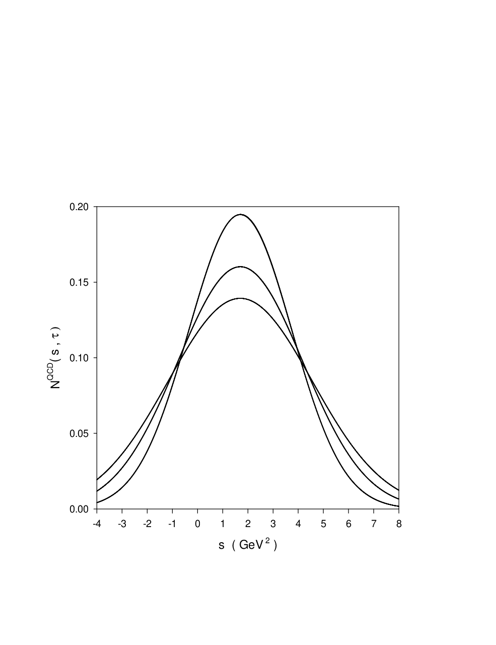
In the case of the diagonal quark and gluonic cases, was constrained by studying the dependence of the value at which the QCD expression for the NGSR reaches its maximum value. This dependence is then compared with that arising from a double-resonance model, and is constrained by optimizing the agreement between them. This procedure for optimizing and determining the resonance parameters has been confirmed by a more numerically-intensive multi-parameter fit of and the resonance parameters [14, 48]. The resonance parameters resulting from our previous analyses of the diagonal gluonic and diagonal quark NGSRs [13, 14, 15] are summarized in Table 1 (the details of the non-diagonal case will be discussed below). The double narrow resonance model results in excellent agreement with the QCD expression as illustrated in Figure 5 [13]; there is no indication of discrepancies that would require a more elaborate phenomenological model (e.g., additional states, resonance widths). For the diagonal NGSRs, the uncertainties associated with the QCD input parameters have been found to be 10% for , and at most for the masses with a correlated effect that leads to a relatively stable mass splitting [13].
| Sum-Rule | (GeV) | (GeV) | () | ||
|---|---|---|---|---|---|
| diagonal: gluonic-gluonic | |||||
| diagonal: - | |||||
| non-diagonal: gluonic- |
The remarkable agreement between the resonance masses resulting from independent analysis of the diagonal gluonic and diagonal NGSRs suggests the existence of states with masses of approximately and that couple to mixtures of gluonium and currents, with the heavier state being slightly more gluonic because of its stronger coupling to gluonic currents and weaker coupling to currents. This consistency of the mass predictions in the two channels is precisely what is expected for hadronic states that couple to both gluonium and quark currents. The results also indicate that the mixing is rather strong (consistent with the conclusions of [9, 10]) because and are not appreciably different, and hence the non-diagonal correlator must also contain clear signals of this strong mixing to validate this scenario. In other words, a definitive signal of states that are -gluonic mixtures is their consistent appearance with the same mass in all three cases (diagonal gluonic, diagonal quark, and non-diagonal gluonic-quark) since such mixtures would necessarily couple to both the gluonic and currents.
Before proceeding with a detailed analysis of the non-diagonal correlator, we consider the approximate scales associated with the couplings of the resonances to the gluonic and scalar currents. The perturbative corrections in the diagonal correlators (see Refs. [13, 14]) imply that
| (71) |
where and respectively denote the resonance couplings to the gluonic and currents and is a characteristic sum-rule energy scale of order . In the simplest single-angle mixing scenario, the non-diagonal correlator will be proportional to where is the mixing angle. The perturbative corrections to the non-diagonal correlator (46) then imply
| (72) |
Combining (71) and (72) then leads to a chirally-suppressed mixing angle for perturbative contributions
| (73) |
A similar chiral suppression exists for the gluon condensate contributions
| (74) |
However, for the quark and mixed condensate contributions we find
| (75) | |||
| (76) |
These estimates illustrate that the chiral-violating condensates avoid the chiral suppression of the mixing angle. However, since the mixing angle generated by the quark condensate will be suppressed compared to the mixed condensate by a factor of . As noted earlier, the mixed condensate is zero at leading order in the non-diagonal pseudoscalar case [16] and hence there is a qualitative distinction between the scalar and pseudoscalar channels. Although it is not as simple to estimate the order of magnitude of the mixing generated by the instanton contributions, one already sees from (76) that a substantive mixing angle is anticipated.
The apparent contradiction between the strong mixing found in the GSRs for the diagonal correlators and the basic perturbative scales in the non-diagonal GSR is therefore resolved by a detailed analysis of the non-diagonal case which demonstrates that the chiral-violating terms (i.e., quark condensate, mixed condensate, and instanton) dominate the perturbative and gluon condensate corrections. We first define the leading chiral terms in (49) as
| (77) |
Figure 6 demonstrates that these leading chiral terms are actually the dominant contribution to the non-diagonal GSR, avoiding the chiral suppression occurring in (73), and obviating the chiral suppression of the mixing angle that would occur for dominantly perturbative corrections. We thus have the intriguing result that the underlying mixing mechanism is fundamentally non-perturbative, i.e., perturbative analyses do not provide the essential phenomenological scales.

Because PCAC fixes the combination , the quark condensate term in (77) is effectively independent of , so in principle could be strongly dependent on . Fig. 7 shows that this is not the case; the NGSR is relatively insensitive to the range (59) for . However, Fig. 8 shows that this is not the case for the LET-sensitive NGSR which exhibits stronger dependence on . Thus we focus our analysis on the NGSR as it is less affected by quark-mass uncertainties. However, it is significant that Figs. 7 and 8 do demonstrate qualitative agreement between and , particularly for at the upper bound of (59).


Our detailed analysis of the non-diagonal GSR begins with an exploration of its consistency with the results of the diagonal cases. In the double narrow resonance model, the non-diagonal NGSR has the form
| (78) | |||
| (79) |
From the analysis of the diagonal cases [13, 14, 15], we have found (see Table 1) , , and
| (80) | |||
| (81) |
Thus the parametrization of the mixed gluonic- system has four couplings of the states to the various currents as in Ref. [11]. The four equations (80) and (81) representing the diagonal results determine the four couplings up to an overall sign, leading to two possible solutions for the non-diagonal case:
| (82) |
Apart from the ambiguity arising from the sign of the couplings, all the phenomenological parameters in the non-diagonal NGSR (78) are determined except for the continuum which can be determined by performing a least-squares fit of the , dependence of (78) in the region and . The best fit for the two cases in (82) are shown in Figs. 9 and 10. From these Figures we see that the positive case in (82) is demonstrably most consistent with the QCD expression.
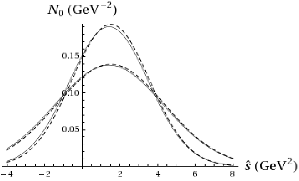
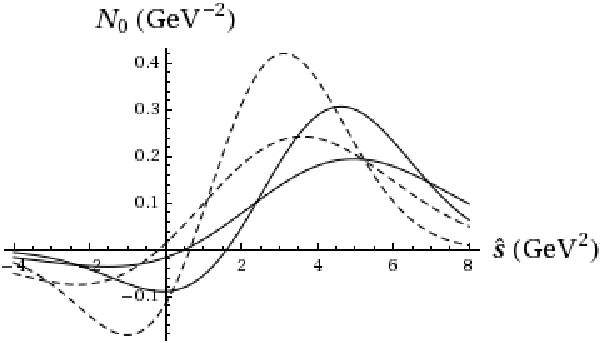
At this point we reach an important conclusion: the non-diagonal GSR is consistent with the results of the diagonal gluonic GSR analyses [13, 14, 15], providing strong evidence for a consistent scenario of mixed gluonic- states with masses of and that couple to mixtures of gluonium and currents, with the heavier state having a slightly larger gluonic coupling. A significant feature of our analysis is the nearly-identical masses that have resulted independently from the diagonal gluonic and diagonal cases. Although we have demonstrated that the non-diagonal case is consistent with these results, an independent analysis of the non-diagonal case is necessary for further confirmation of this gluonic- mixing scenario.
The moments (67)–(69) will be used to determine the QCD predictions of the resonance parameters arising from the non-diagonal NGSR . In Figs. 11 and 12 we show the , dependence of these moments. As required in a reliable sum-rule analysis, the resulting resonance parameters show almost no dependence. The predicted value of the resonance parameters is then obtained from the point where they are stable against variations in . This point of stability is approximately in all cases and is comparable in scale to that resulting from the diagonal analysis (see Table 1), confirming the reliability of the procedure. The results of the analysis of the non-diagonal NGSR are given in Table 1. Although the theoretical uncertainties for the non-diagonal sum-rule have not yet been discussed, it is evident that the independent predictions of the masses from all possible sum-rules show exceptional agreement, particularly for the heavier state. Furthermore, the prediction from the non-diagonal sum-rule is in excellent agreement with the positive solution of Eq. (82) emerging from the diagonal sum-rules.


For the non-diagonal NGSR, the double narrow resonance model results in excellent agreement with the QCD expression as illustrated in Figure 13; as in the diagonal case (see Fig. 5) there is no indication of discrepancies that would require a more elaborate phenomenological model (e.g., additional states, resonance widths). As a further diagnostic, Fig. 14 illustrates that the optimized value leads to excellent agreement between the dependence of the QCD expression and its expected dependence (70) from the two resonance model: a straight line with slope and a positive intercept.


Because the non-diagonal sum-rule is dominated by the chiral-violating contributions, the Table 1 predictions of the resonance parameters only depend on the quark mass, mixed condensate, instanton size, and instanton density. The quantity is most dependent on and , whereas and are most dependent on . By comparison, the resonance parameters are relatively unaffected by uncertainties in the mixed condensate and . In aggregate, the resulting uncertainties in the mass parameters are comparable to those found in the diagonal case: approximately with a correlated effect that leads to a relatively stable mass splitting . However, in comparison to the diagonal analyses, the couplings have greater sensitivity to the input parameters in the non-diagonal case, with an uncertainty in of approximately . Across the entire parameter space considered, continues to stabilize at the same value for all the resonance parameters, demonstrating that our methodology is robust.
Taking into account the uncertainties in the values of the resonance parameters for the diagonal and non-diagonal NGSRs associated with Table 1, we see that the non-diagonal case leads to predictions that are consistent with those of the diagonal analyses, so that all possible GSRs of gluonic and currents independently confirm the existence of two states with approximate masses of and that couple to mixtures of gluonium and currents. In particular, there is excellent agreement between the central value obtained from analysis of the non-diagonal NGSR and the positive solution in Eq. (82) resulting from the diagonal NGSRs.
Another inherent source of uncertainty in our analysis is the narrow resonance approximation. One can qualitatively model the effect of resonance widths and kinematic distortions by studying their effect on the moments (63)–(65). For example, a Gaussian resonance (which introduces an effective Breit-Wigner width ) with a kinematic distortion [44, 47] can be modelled by decreasing the QCD values of the moments systematically as a function of the ratio [13] and then exploring the effect on the resonance parameters as a series in . The leading-order deviations of and from their narrow-width values are proportional to with a negative coefficient of in GeV units. From this we can conclude that the narrow-width approximation tends to overestimate the masses if the underlying resonances are broad and kinematically-skewed (see e.g., [49] for similar conclusions in other contexts). In this situation, the mass predictions in Table 1 can be conservatively interpreted as an upper bound on the masses in a more complicated models [44, 47].
We now examine the pattern of mixing of the couplings for these states as contained in the quantities for the various cases. If the couplings obey a single-angle mixing pattern, then one would expect . Although such a scenario could be possible given the 10% uncertainty in these quantities in Table 1, the non-diagonal case provides a more sensitive test because single-angle mixing leads to
| (83) |
In this situation, the integral of the right-hand side of (83) is zero which then requires in (51). A value of can be found to satisfy this constraint over the considered range . However, as shown in Fig. 15 the , dependence of the QCD expression is not consistent with mass scales and . We thus conclude that the pattern of mixing for the couplings is not consistently described by a single mixing angle, and hence the situation must be similar to the two-angle scenario that has been found for the couplings (decay constants) of the - system in the singlet-octet basis [50]. Implicitly this is the same result found in [8, 11], where four independent couplings are found necessary in the study of the mixed gluonic- system rather than the three-parameter system of two couplings and one mixing angle. Following Ref. [8], we then define an effective mixing angle
| (84) |
where and respectively correspond to the states with mass and . Taking into account the uncertainties in the Table 1 values leads to . Thus we find that the effective mixing angle corresponds to nearly maximal mixing () where each of the two states are equally coupled to the and gluonic currents, a result in excellent agreement with the conclusions of [9, 10]. The deviation of our effective mixing angle from the maximal angle indicates that the heavier () state is somewhat more gluonic in comparison to the lighter () state .

5 Discussion and Conclusions
Gaussian QCD sum-rules are able to probe hadronic spectral functions over a broad range of energy, and are thus ideally suited to exploring the possibility of states that couple to mixtures of gluonium and currents exist amongst the light scalar mesons. We have studied the NGSRs for all possible combinations of scalar gluonic and scalar (non-strange) currents (diagonal gluonic, diagonal , and non-diagonal -gluonic) and find that all three cases independently predict the existence of two states with masses of approximately and . This is precisely what one would expect from hadronic states that couple to mixtures of gluonium and currents. Given the uncertainties in our mass predictions, it is not clear whether our lighter state should be interpreted as the or (at the heavier end of its range [1]) and it is also not clear whether the heavier state should be interpreted as the or the . However, because the approximate mass splitting between the states is relatively stable under QCD uncertainties, our results do suggest identifying either the lighter pair of states [ and ] or the heavier pair [ and ] as states coupling to mixtures of gluonium- currents.
The non-diagonal sum-rule provides important insights into the mixing of the and gluonic aspects of these two states. Because of chiral suppression factors associated with the light (non-strange) quarks, perturbative effects are unable to generate any significant amount of mixing. However, the chiral-violating contributions of the quark condensate, mixed condensate, and instantons do not suffer from this chiral suppression and provide the dominant contribution to the non-diagonal correlation function, implying that mixing of gluonic and degrees of freedom has a non-perturbative origin. Qualitatively, this conclusion is similar to that obtained for glueball decays [21] and to that of Ref. [51] which demonstrated that instantons can lead to a significant mixing between glueballs and (heavy quark) mesons in the pseudoscalar channel.
The state couplings that result from the analysis of the various GSRs provide an additional means to examine the self-consistency of the scenario of two states with masses of approximately and that couple to mixtures of and gluonic currents. In particular, the relative couplings between the states in the non-diagonal case is constrained by the relative couplings in the diagonal cases. The independent prediction of these couplings from the non-diagonal NGSR is found to satisfy this constraint extremely well, providing strong evidence for the validity of the mixing scenario.
The state couplings also provide a means to study the pattern of mixing associated with the couplings to gluonic and currents. The resulting pattern is similar to the two-angle mixing that occurs for the couplings (decay constants) for the - system in the singlet-octet basis [50], and result in an effective mixing angle of in excellent agreement with the sum-rule analyses of Refs. [9, 10]. Because this mixing angle is in the region near maximal mixing (), there is only a slight preference for the heavier state to couple to gluonic currents and a concomitantly slight preference for the lighter state to couple to currents. Indeed, the existence of such strong mixing implies that qualitative features that would distinguish pure gluonic and states would be obscured for strongly-mixed states and the experimental signal of gluonium would thus be elusive.
In summary, our results provide strong QCD evidence to support the scenario where the mixing of and gluonium is manifested in the scalar hadronic spectrum as a lighter state on the order of and a heavier state on the order of [4, 6, 8, 9, 10, 11, 12, 15]. In particular, our conclusion that there exists a strong mixing between gluonium and states is similar to the results from a variety of approaches [6, 8, 9, 10] and our result for the heavier state’s preference for gluonic channels provides QCD support for the findings of a large gluonic component of the [2, 3].
Acknowledgements: The authors are grateful for financial support from the Natural Sciences and Engineering Research Council of Canada (NSERC). Many thanks to Hong-Ying Jin for helpful discussions. TGS dedicates this work to the memory of Victor Elias.
References
- [1] W.-M. Yao et al., J. Phys. G 33 (2006) 1.
- [2]
F.E. Close, A. Kirk, Phys. Lett. B483 (2000) 245;
De-Min Li, Hong Yu, Qi-Xing Shen, Mod. Phys. Lett. A15 (2000) 1781. - [3]
C. Amsler and F.E. Close, Phys. Rev. D53 (1996) 295;
L. Burakovsky and P.R. Page, Phys. Rev. D59 (1999) 014022;
F.E. Close, Qiang Zhao, Phys. Rev. D71 (2005) 094022. - [4]
A.H. Fariborz, Phys. Rev. D74 (2006) 054030;
A.H. Fariborz, Int. J. Mod. Phys. A19 (2004) 2095. - [5] M. Albaladejo, J.A. Oller, Phys. Rev. Lett. 101 (2008) 252002.
- [6]
P. Minkowski, W. Ochs, Eur. Phys. J. C9 (1999) 283;
Peter Minkowski, Wolfgang Ochs, arXiv:hep-ph/0209225. - [7]
C.J. Morningstar, M. Peardon, Phys. Rev. D60 (1999) 034509;
A. Vaccarino, D. Weingarten, Phys. Rev. D60 (1999) 114501;
Y. Chen et al, Phys. Rev. D73 (2006) 014516. - [8] UKQCD Collaboration: A. Hart, C. McNeile, C. Michael, J. Pickavance, Phys. Rev. D74 (2006) 114504.
- [9] S. Narison, Nucl. Phys. B509 (1998) 312.
- [10]
G. Mennessier, S. Narison, N. Paver, Phys. Lett. B158 (1985) 153;
S. Narison, G. Veneziano, Int. J. Mod. Phys. A4 (1989) 2751;
A. Bramon, S. Narison, Mod. Phys. Lett. A4 (1989) 1113;
S. Narison, Phys. Rev. D73 (2006) 114024. - [11] Tao Huang, Hong Ying Jin and Ai-lin Zhang, Phys. Rev. D59 (1998) 034026.
- [12] L.S. Kisslinger, J. Gardner and C. Vanderstraeten, Phys. Lett. B410 (1997) 1.
- [13] D. Harnett, T.G. Steele, Nucl. Phys. A695 (2001) 205.
- [14] G. Orlandini, T.G. Steele, D. Harnett, Nucl. Phys. A686 (2001) 261.
- [15] T.G. Steele, D. Harnett, G. Orlandini, AIP Conf. Proc. 688 (2004) 128 [arXiv:hep-ph/0308074].
- [16] S. Narison, N. Pak, N. Paver, Phys. Lett. B147 (1984) 162.
- [17] M.S. Chanowitz, Phys. Rev. Lett. 95 (2005) 172001.
- [18] V.A. Novikov, M.A. Shifman, A.I. Vainshtein and V.I. Zakharov, Nucl. Phys. B191 (1981) 301.
- [19] S. Narison, QCD as a Theory of Hadrons (Cambridge University Press) 2004.
- [20] Hilmar Forkel, Phys. Rev. D71 (2005) 054008.
- [21] Z.F. Zhang, H.Y. Jin, arXiv:hep-ph/0511252v3.
- [22] R.A. Bertlmann, G. Launer, E. de Rafael, Nucl. Phys. B250 (1985) 61.
- [23] P. Pascual and R. Tarrach, Phys. Lett. B113 (1982) 495.
- [24]
N.K. Nielsen, Nucl. Phys. B120 (1977) 212;
J.C. Collins, A. Duncan, S.D. Joglekar, Phys. Rev. D16 (1977) 438. - [25] R. Tarrach, Nucl. Phys. B196 (1982) 45.
- [26] J.I. Latorre, S. Narison, S. Paban, Phys. Lett. B191 (1987) 437.
- [27] E.V. Shuryak, Nucl. Phys. B203 (1982) 93.
- [28]
H. Forkel, Phys. Rev. D64 (2001) 034015;
D. Harnett, T.G. Steele, V. Elias, Nucl. Phys. A686 (2001) 393. - [29] D. Binosi and L. Theußl, Comp. Phys. Comm. 161 (2004) 76.
- [30] M.A. Shifman, A.I. Vainshtein and V.I. Zakharov, Nucl. Phys. B147 (1979) 385, 448.
- [31] M. Jamin, M. Muenz, Z. Phys. C60 (1993) 569.
- [32] E. Bagan, J.I. Latorre, P. Pascual, Z. Phys. C32 (1986) 43.
- [33] E. Bagan, M.R. Ahmady, V. Elias, T.G. Steele, Z. Phys. C61 (1994) 157.
- [34] V. Elias, T.G. Steele, M.D. Scadron, Phys. Rev. D38 (1988) 1584.
- [35]
A. Belavin, A. Polyakov, A. Schwartz and Y. Tyupkin,
Phys. Lett. B59 (1975) 85;
G. ’t Hooft, Phys. Rev. D14 (1976) 3432. - [36] T. Schäefer and E.V. Shuryak, Phys. Rev. Lett. 75 (1995) 1707.
- [37] M. Abramowitz and I.E. Stegun, Mathematical Functions with Formulas, Graphs, and Mathematical Tables (National Bureau of Standards Applied Mathematics Series, Washington) 1972.
- [38] S. Narison, Nucl. Phys. B (Proc. Supp.) 54A (1997) 238.
- [39] H.G. Dosch, M. Jamin and S. Narison, Phys. Lett. B220 (1989) 251.
- [40] V.A. Novikov, M.A. Shifman, A.I. Vainshtein and V.I. Zakharov, Nucl. Phys. B165 (1980) 67.
- [41] L.S. Kisslinger, M.B. Johnson, Phys. Lett. B523 (2001) 127.
- [42]
S. Narison, Z. Phys. C26 (1984) 209;
H. Forkel, Phys. Rev. D71 (2005) 054008. - [43] E. Bagan and T.G. Steele, Phys. Lett. B243 (1990) 413.
- [44]
J. Bordes, V. Gimènez and J.A. Peñarrocha, Phys. Lett. B223 (1989) 251;
J.L. Liu and D. Liu, J. Phys. G19 (1993) 373. - [45] N.V. Krasnikov, A.A. Pivovarov, N.N. Tavkhelidze, Z. Phys. C19 (1983) 301.
- [46] M.A. Shifman, Z. Phys. C9 (1981) 347.
- [47] C.A. Dominguez and N. Paver, Z. Phys. C31 (1986) 591.
- [48] Ailin Zhang, T.G. Steele, Nucl. Phys. A728 (2003) 165.
- [49] V. Elias, A.H. Fariborz, Fang Shi, T.G. Steele, Nucl. Phys. A633 (1998) 279.
- [50]
A.V. Kisselev, V.A. Petrov, Z. Phys. C58 (1993) 595;
Th. Feldmann, P. Kroll, B. Stech, Phys. Rev. D58 (1998) 114006;
Th. Feldmann, P. Kroll, B. Stech, Phys. Lett. B449 (1999) 339. - [51] N. Kochelev and Dong-Pil Min, Phys. Rev. D72 (2005) 097502.