Probing the quantum coherence of a nanomechanical resonator using a superconducting qubit: I. Echo scheme
Abstract
We propose a scheme in which the quantum coherence of a nanomechanical resonator can be probed using a superconducting qubit. We consider a mechanical resonator coupled capacitively to a Cooper-pair box and assume that the superconducting qubit is tuned to the degeneracy point so that its coherence time is maximised and the electro-mechanical coupling can be approximated by a dispersive Hamiltonian. When the qubit is prepared in a superposition of states this drives the mechanical resonator progressively into a superposition which in turn leads to apparent decoherence of the qubit. Applying a suitable control pulse to the qubit allows its population to be inverted resulting in a reversal of the resonator dynamics. However, the resonator’s interactions with its environment mean that the dynamics is not completely reversible. We show that this irreversibility is largely due to the decoherence of the mechanical resonator and can be inferred from appropriate measurements on the qubit alone. Using estimates for the parameters involved based on a specific realization of the system we show that it should be possible to carry out this scheme with existing device technology.
1 Introduction
One way of exploring the quantum coherence properties of a nanomechanical resonator is to couple it to a qubit formed by a solid-state two-level system (TLS). Coupling to an isolated harmonic oscillator can initially cause an apparent loss of phase coherence in the qubit if the oscillator is driven into a superposition of orthogonal states, but signatures of the overall coherence of the full system (i.e. oscillator and TLS together) can be found in the subsequent dynamics of the TLS. However, if instead the qubit is coupled to a harmonic oscillator which is in turn coupled to a bath, then the effective dynamics of the TLS and oscillator will now be different and the loss of the oscillator’s coherence due to the bath will be manifest in the dynamics of the TLS [1, 2, 3].
From a theoretical point of view it is relatively straightforward to devise simple schemes based on these principles to probe the rate at which the environment causes decoherence of an oscillator [4]. Indeed, exactly this kind of approach has been used very successfully in the field of cavity quantum electrodynamics (cQED) to probe the quantum coherence of a mode of the electromagnetic field by examining its influence on effectively two-level atoms [5, 6, 7]. Similar experiments have also been carried out successfully on trapped ions with the internal electronic state of the ion playing the role of the two-level system and the ion’s motional state the oscillator [8, 9, 10].
The development of relatively large and well controlled quantum coherent TLSs in the solid-state, such as superconducting circuits designed to act as qubits, seems to offer a way to perform analogous experiments with nanomechanical resonators [1, 2]. Furthermore, recent experiments have demonstrated that it is possible to recreate many of the features of traditional optical cQED in the solid state using a superconducting qubit coupled to a superconducting resonator [11, 12]. Since nanomechanical resonators are typically a few microns in length and contain macroscopic numbers of atoms, producing a quantum superposition of spatially separated states in such systems and monitoring its progressive loss of coherence (due to interactions with its environment) would represent an important increase in size of the system involved compared to superpositions of ions and light [13, 14]. However, performing quantum coherent experiments using a nanomechanical resonator is likely to be more difficult than with a superconducting one as nanomechanical resonators are generally much lower in frequency.
In order to understand the practical difficulties entailed in using a superconducting qubit to probe the decoherence of a nanomechanical resonator we briefly review the apparent constraints which any such scheme must satisfy. First of all, the superconducting qubit must remain sufficiently coherent that the influence of the mechanical resonator’s environment can be clearly discerned in its dynamics. Secondly, it will be desirable to couple the TLS and resonator as strongly as possible since the signal(s) of coherence and/or decoherence in the mechanical resonator measurable in the TLS will become clearer the larger the coupling between the TLS and resonator. Finally, unless impressive cooling of the resonator can be achieved, the experiments will always have to contend with the competing effect of phase smearing arising from the range of oscillator states (and their associated phases) in the thermal ensemble of the oscillator. Again the relatively low frequencies of mechanical resonators make this more of a problem than it would be in the superconducting case. Note that in practice there is no simple way of designing a double clamped beam resonator to optimize all of these constraints at once11 1 One interesting way to avoid the problems posed by the relatively low frequency of flexural-mode mechanical resonators is to use a different type of mechanical system, such as dilational disk resonators which can have frequencies well beyond 1 GHz [15]. Here, however, we will confine our attention to the conventional mechanical resonators formed by doubly clamped beams.. For example, in most realizations the TLS-resonator coupling will increase as the resonator is made larger, but enlargement of the resonator will inevitably reduce its fundamental frequency.
In this paper we describe how a dispersive interaction between a superconducting qubit and a nanomechanical resonator can be used to produce superpositions of the resonator state and how the coherence of this superposition can then be probed by measuring the state of the TLS. We identify the relatively short coherence times of the superconducting qubit as the most serious constraint on these types of scheme and hence assume that the TLS is tuned to operate at a point where its coherence is maximized; it is this choice of operating point which leads to a dispersive coupling between the TLS and the resonator. Although the dispersive interaction is relatively weak, we find that the effect of the TLS on the resonator can be amplified by preparing the latter in a state with large amplitude. We explore in detail the quantum dynamics of the resonator and TLS including the effects of the inevitably mixed initial state of the resonator and the interaction with the environment. In assessing the extent to which the schemes we propose can be carried out in practice we make use of the analysis in the companion reference [16], which considers how sufficiently strong coupling between a nanomechanical resonator and a superconducting qubit can be best achieved without degrading the coherence of the qubit.
Our work builds on and extends previous studies of similar systems [1, 2, 17, 3, 18]. In particular, we believe that the scheme outlined here represents an important improvement on that proposed by us in Ref. [1] in a number of respects. Most importantly, the scheme we propose here is more likely to be practicable as it is designed to be performed at the degeneracy point of the qubit where it remains coherent for at least an order of magnitude longer [19] than the operating point considered in [1]. Furthermore, the scheme is much more flexible in the sense that it would be possible to vary several of the important parameters systematically (such as the phase space separation of the resonator states involved and the duration of the superposition). This would be an important advantage in interpreting the results of this type of experiment, since the nature of the mechanical resonator’s environment is not well understood [20] and in a sense the purpose of the experiment we propose would be to provide empirical information about it.
This paper is organised as follows. In section 2 we introduce the generic Hamiltonian for the superconducting qubit-resonator systems which we will work with here. We discuss the practical constraints which dictate our choice of operating regime and introduce the effective (dispersive) Hamiltonian which is valid when the mechanical resonator is much slower than the superconducting circuit. Next in section 3 we describe how the dispersive interaction can create states which involve superpositions of spatially separated states of the mechanical resonator so that measurements on the TLS alone show an apparent initial loss of coherence. We show that the TLS coherence can be recovered (recoherence) in a controlled way using a particular choice of control pulses. In section 4 we calculate how the presence of the environment of both the mechanical resonator and the qubit itself affects recoherence. We then consider the values of the various parameters which are likely to be practicable in present or near future experiments in section 5. Then in section 6, we present calculations of the behaviour of the recoherences for a range of practicable parameter values. Finally, section 7 contains a discussion of our results and our conclusions. The Appendix contains further details on some of our calculations.
2 Resonator-TLS Effective Hamiltonian
2.1 Operating Regime
The generic Hamiltonian for the superconducting TLS and mechanical resonator which we consider here is,
| (1) |
where the qubit energy scales and depend on the details of the specific superconducting system considered, is the resonator frequency, is the strength of the resonator-TLS coupling, and the operators act on the TLS while act on the resonator. The mechanical resonator is assumed to be the fundamental flexural mode of a suspended doubly-clamped beam. The coupling between the TLS and the mechanical resonator is implicitly assumed to be weak in the sense that only linear (in the resonator position coordinate) coupling needs to be considered. The TLS states are defined as and so that e.g. .
This Hamiltonian is derived in Ref. [16] for the specific cases of either a Cooper pair box (CPB) with an island which is suspended to form the mechanical resonator, or a flux qubit (again with suspended segment that forms the mechanical resonator). In each case the qubit is also assumed to be fabricated close to the centre electrode of a superconducting microwave coplanar waveguide (CPW) resonator. The CPW resonator provides a way to both measure and manipulate the qubit state, as well as a means to drive the mechanical resonator into an initial state which has a large amplitude. Although both the mechanical resonator and the qubit are also coupled to the CPW resonator in this system as just stated, we will not include the latter explicitly in this article, assuming that it is unpopulated (i.e. it is at or close to the vacuum state), except initially when used to drive the mechanical resonator [16] and for the short periods when it is used to manipulate the state of the qubit. Population of the CPW resonator is required when measuring the qubit state, but at this stage disruption to the mechanical system and dephasing of the qubit are unimportant so long as the measurement can still be performed with high fidelity, which we will assume is the case. For a CPB the states correspond to different charge states and the coupling between the TLS and the resonator is capacitive. In contrast, when the Hamiltonian [equation (1)] is realized with a flux qubit, the coupling between the TLS and the mechanical resonator is inductive and the relevant qubit states are of current circulating in opposite directions [2, 16, 21].
The best coherence times for both superconducting charge and flux based qubits are achieved at the degeneracy point where . Away from the degeneracy point, experiments [19] have demonstrated that the coherence times of superconducting qubits decrease by orders of magnitude. We regard the coherence of the superconducting TLS as the primary constraint and hence we choose to operate the TLS at its degeneracy point when probing the resonator’s coherence. Another important constraint arising from the use of the superconducting TLS is the need to avoid thermal mixing of the two states involved. In practice, for experiments performed at temperatures of order 20 mK this means that we will require energy separations between the two states (i.e. when working at the degeneracy point) in the superconducting TLS that are much larger than the thermal energy scale. Experiments [22] using a CPB (coupled to a superconducting CPW resonator for state control and read-out) achieved coherence () times of up to s (operating at the degeneracy point) and relaxation times () of about s with GHz and we take these as indicative of the current practical limitations. Note that even longer coherence times of up to s have been reported for experiments on CPBs using an echo technique in which the TLS state is inverted mid-way through the experiment[23]
In terms of the mechanical resonator, we will consider beam structures which are fabricated by under-etching a bulk substrate or metallic film. The fundamental (flexural) mode frequencies of such devices can in practice be as high as GHz [24], but because the electro-mechanical coupling, , (in equation 1) for such modes increases with the length of the beam, , (for both capacitive and inductive couplings [16]) whereas the frequency clearly decreases with increasing , it is clear that high frequencies can only be achieved at the expense of very weak couplings [16, 1, 2]. Nanomechanical resonators have already been fabricated in close proximity to superconducting structures [25], but with mechanical frequencies MHz. We therefore assume that the mechanical frequency will be much lower than the energy scale of the qubit, i.e. . Having made this assumption of a wide separation of time-scales for the mechanical and superconducting elements we can proceed to derive a simpler effective Hamiltonian which is valid in this regime.22 2 Note that the CPW resonator used to manipulate the CPB state will have a frequency which is close to and hence is also very far from the mechanical frequency.
2.2 Adiabatic limit
When , is tuned to zero it is convenient to rewrite the Hamiltonian in terms of a new basis for the qubit. Defining new basis states,
| (2) |
we can write the Hamiltonian (1) for as
| (3) |
where the new spin operators are defined in terms of the new basis states.
We proceed by exploiting the separation in time-scales to make an adiabatic approximation [2, 26, 27, 28]. Since the mechanical resonator will generally be in a Gaussian state of large amplitude, in what follows it is reasonable to take a semi-classical approach [26]. We initially assume that the mechanical resonator is at a fixed position and use this to calculate the eigenvalues of the TLS, these are then used to calculate an effective Hamiltonian for the oscillator. With the resonator at position the Hamiltonian of the TLS is (using equation 3):
| (4) |
where . The eigenvalues of the TLS are now . For sufficiently weak coupling i.e. , we can expand the eigenvalues to lowest order
| (5) |
The evolution of the mechanical system over time then causes a weak position dependent (and hence ultimately time dependent) perturbation to the eigenstates of the TLS. In the adiabatic approximation the wide separation of time-scales and weak coupling mean that the TLS evolves smoothly within each eigenstate with its dynamics arising from changes in time of the eigenstates themselves, rather than any transitions between different eigenstates.
Labeling the instantaneous eigenstates of equation (4) as and , we can write down the effective Hamiltonian felt by the oscillator for the TLS confined to one of its eigenstates as,
| (6) |
Therefore within the framework of the adiabatic approximation we can write down the following model Hamiltonian for the system,
| (7) |
We have dropped the distinction between perturbed and unperturbed eigenstates as it does not play a role in what follows.
Assuming that the coupling term is a weak perturbation (i.e. assuming ), we can also make the rotating wave approximation in which the terms and are dropped [2]. The final result of these approximations is the following dispersive Hamiltonian for the TLS-resonator system,
| (8) |
where . A key feature of this Hamiltonian is that the perturbation of the oscillator commutes with the unperturbed Hamiltonian (i.e. it is a QND Hamiltonian). This feature is exploited in schemes to measure the number state of a resonator using a superconducting qubit [29, 30, 31] and it also plays an important role in what follows here. Note that this Hamiltonian can also be obtained from equation (3) via a range of other approaches [7, 17, 32, 30, 33].
3 Coherent oscillations and recoherences: simple description
The dispersive Hamiltonian shifts the mechanical frequency in a way that depends on the state of the TLS. This interaction can be used to probe the quantum coherence of the mechanical resonator. The idea is to perform a Ramsey interference [7] experiment in which the qubit is prepared in a superposition of its eigenstates states using a control pulse, this superposition is then allowed to interact with the resonator for a time before a second pulse is applied to the qubit and then a measurement of its state is performed. For an isolated TLS the probability of finding the system in one or other of its eigenstates at the end of the experiment will oscillate between zero and unity as a function of the time between the two control pulses. When the mechanical resonator is present the interaction with the superposition of TLS states leads to an overall superposition of states involving spatially separated mechanical states. For a sufficiently strong interaction, the separation of the resonator states coupled to the qubit states leads to a strong suppression of the oscillations in the final qubit state measurements. The coherence of the resonator can be inferred by inverting the state of the TLS midway between the two original control pulses. The scheme is illustrated schematically in figure 1. In the absence of the resonator’s environment, such an inversion should lead to a reversal of its dynamics and hence the recovery of the oscillations in the final TLS state measurement [6]. Very similar schemes have been demonstrated in optical systems [7].
In what follows, we will assume that it is possible to measure the state of the TLS within the basis and to rotate its state by applying transformations of the form with a parameter that can be controlled to a high degree of precision. These requirements are readily met in the system of a charge or flux qubit (with suspended segment forming a mechanical resonator) coupled to a superconducting CPW resonator described in Ref. [16], which we consider here. The TLS state is determined by measuring the transmission of an off-resonant pulse applied to the CPW resonator, while rotation of the TLS is performed by applying almost-resonant pulses to the CPW resonator and making use of the resulting Rabi oscillations [32, 22].
We will begin by considering the simple though unrealistic case of an isolated resonator which is initially prepared in a coherent state, . The effects of the environment on the evolution of the coupled TLS-resonator device and the types of initial (mixtures of) states of the oscillator that can be prepared in practice are addressed in later sections. We assume that the TLS system is in its ground state , hence the total initial state is . Application of an appropriate control pulse to rotate the state of the TLS by produces a superposition of TLS states. Since the rotation of the TLS will in practice be very fast compared to the mechanical period we can neglect any evolution of the mechanical resonator during the pulse and hence write the total state of the system after the pulse as with
| (9) |
Starting with this initial state at , the dispersive interaction [equation (8)] leads to the following joint state after time ,
| (10) |
where
| (11) | |||||
| (12) |
The resonator evolution in phase space during this period is illustrated in figure 1b. The next step is to perform a second rotation on the TLS, leading to the state
| (13) |
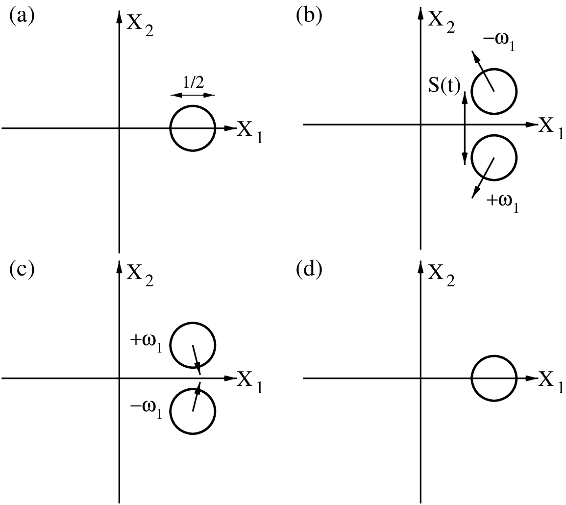
Finally, the state of the TLS is measured in the basis. The probability of finding the TLS in state for a period of evolution between the two control pulses is
| (14) |
The overlap is readily evaluated,
| (15) |
The final result for is thus,
| (16) |
Note that this function depends only on the amplitude of the initial mechanical state, not its phase.
The behaviour of is easy to understand. Without any coupling to the resonator the coherent oscillations in the TLS state mean that the probability oscillates over time between zero and unity with a period 33 3 Note that in practice the pulses used to rotate the state of the TLS are chosen to be slightly off-resonant. As a result a stroboscopic observation of the oscillations in can be made which replaces the very fast oscillations at frequency with much slower (and hence easier to observe) ones at the chosen de-tuning frequency [7, 34, 22], we neglect this detail here as our primary interest is not in the frequency of the oscillations but in their amplitude. a key indicator of the quantum coherence of the TLS [22]. For sufficiently strong coupling, the resonator causes a relatively rapid reduction in the amplitude of the oscillations as a function of time leading to a period where , implying that the resonator decoheres the TLS. However, because the resonator is a periodic system and is itself coherent, the oscillations in reappear, giving rise to so-called recoherence, for [2].
Although recoherence does occur naturally after a time it is preferable to use an approach where the time between coherences can be varied systematically. This is readily achieved using a spin echo technique to induce recoherence at a chosen time. This type of approach was used with great success in optical cQED experiments [6] as well as experiments on superconducting circuits [12, 23].
3.1 Echo technique
For the spin echo sequence we again start with the system in the state (equation 9) and allow it to evolve as before for a time so that,
| (17) |
Next we apply a control pulse to the TLS which effectively inverts the populations of the two eigenstates [this corresponds to the unitary operation with ]. Thus, just after the pulse we have
| (18) |
We now allow the system to evolve for a further time , after which the resulting state of the system will be
| (19) |
where now,
| (20) | |||||
| (21) |
Note that the simplicity of this expression relies on the fact that the perturbed resonator Hamiltonian commutes with the unperturbed one44 4 Note, however, that with an appropriate choice of control pulse at the idea of an echo experiment is not limited to systems with dispersive Hamiltonians. This type of experiment has been performed for systems with a Jaynes-Cummings type interaction [6]., thus we find
| (22) |
Carrying out a final rotation of the TLS state (with ) the final overall probability of finding it in state is given by
| (23) |
The probability is zero at when , this is because at this instant the oscillator states associated with each of the qubit states are the same so that the effect of the pulses is simply to rotate the qubit through a total of . To examine the apparent coherence of the qubit we can define the envelope of the oscillations in ,
| (24) | |||||
| (25) |
The envelope of the oscillations is unity when signifying the recoherence of the qubit. Thus we can use the echo approach to induce recoherences in the qubit dynamics whenever we choose by tuning . We note that this particular approach also has the advantage that inverting the state of the TLS at can lead to an increase in the effective coherence of the TLS as measured at as it eliminates dephasing effects arising from fluctuations in the TLS energy level spacings which occur between different experimental runs [23].
3.2 State separation and entanglement
After evolving for a time (and without any inversion of the TLS states), the two coherent states of the resonator that (together with the TLS states) form a superposition are [equation (12)] and they have a separation in phase space given by
| (26) | |||||
| (27) |
where etc, and the phase space operators are defined by and . Because we are dealing with a pure state of the TLS and resonator we can also obtain the entanglement of the system, , by calculating the von Neumann entropy of the reduced density matrix (of either the resonator or the TLS)55 5 Note that the entanglement dynamics of this system was studied very recently for mixed states [35]. Evaluating this we find that it is entirely determined by the phase space separation of the resonator states [13],
| (28) |
where . The entanglement rapidly saturates at its maximum value of unity as the separation is increased: it reaches about 0.75 for and is already very close to unity for . Note that the decay of the qubit oscillations also depends on alone: we can rewrite equation (16) as,
| (29) |
where the (real) phase is defined as .
The aim of these simple calculations is just to show that the separation of the resonator states in phase space provides an important figure of merit for the kind of experiment we have in mind. The diameter of the ‘uncertainty circle’ [33] for a coherent state is 1/2 and so one basic (though somewhat arbitrary) criterion for producing a distinguishable superposition of resonator states is to require . Although according to equation (27) the largest separation is achieved when , in practice the limited coherence times available for the TLS mean that the evolution times will be such that and hence we can approximate . If we use the spin echo approach then the maximum separation will be achieved at just before the TLS state is inverted and hence to achieve a meaningful superposition we would need to have . The details of how a driven resonator state could be prepared in practice for the qubit-mechanical resonator system in which the mechanical component is formed by suspending part of the qubit circuit is considered in reference [16]; we will make use of the results obtained there when considering what kind of initial mechanical state could be prepared in practice, but for now we point out the crucial role played by the magnitude of the initial coherent state, . The size of resonator state superposition produced depends through on the initial state of the oscillator. This provides us with a way of overcoming the weak TLS-resonator coupling and the wide separation of their time scales: by preparing the resonator in a state with large enough we can overcome the very weak interaction with the qubit to nevertheless produce relatively large superpositions over the relatively short times during which the TLS remains coherent. On the other hand, unless we start with a state with non-zero then will be zero throughout (and no entanglement will be produced).
4 Role of the resonator’s environment
We now consider the effect which the resonator’s environment has on the recoherences in the qubit. The interaction between the resonator and its surroundings is typically modelled by including a bath of oscillators that are weakly coupled to the resonator. This approach is the one followed in quantum optics and although it is not clear to what extent it represents an actual nanomechanical resonator’s environment [20], it can at least be justified in the idealised case where dissipation in the collective mechanical mode which forms the resonator is due only to coupling to the bulk phonon modes in the supports of the resonator [36]. In this simplified description the effects of the bath on the ‘system’ resonator can parameterized by a damping rate for the resonator and a temperature , which can be expressed in terms of the average number of the quanta the resonator would have if it were in equilibrium with the bath,
| (30) |
For sufficiently high temperatures () the master equation for the mechanical resonator and qubit including the dissipative effects of the resonator’s environment can be modelled using the quantum optical damping kernel [37],
| (31) |
where
| (32) |
Assuming that the oscillator damping is very weak () we can further simply the dissipative part of the master equation by using the rotating wave approximation,
| (33) |
We stress again that we use this damping kernel here to provide a simple illustrative estimate of the dissipative dynamics of the mechanical resonator. The true form of the mechanical damping kernel remains somewhat uncertain and one of the aims of the experiments we propose would be to obtain empirical information about it.
The superconducting qubit is also subject to decoherence due to interactions with other degrees of freedom in the system apart from the mechanical resonator [19]. The dissipative dynamics of such systems can be characterised by the relaxation times in the equations of motion for the diagonal and off-diagonal components of the TLS density operator. The decay of the excited state population of the TLS is described by , while the decay of the TLS coherence is described by . In practice, times have been typically an order of magnitude larger than times [22]. Since we will only consider total evolution times (before measurement) of the system that are shorter than , we therefore will always have and hence can neglect relaxation of the TLS in what follows. The master equation for the system [equation (31)] can be written in terms of the components etc, incorporating a finite time as follows,
| (34) | |||||
| (35) | |||||
| (36) | |||||
where .
We assume that immediately after the first control pulse is applied to the TLS the state of the system is given by
| (37) |
where and is a displaced thermal density operator [38] for the resonator defined by
| (38) | |||||
| (39) |
where is the displacement operator and we have defined in the last line. The undisplaced thermal density operator is
| (40) |
where . We have chosen to specify a temperature for the initial state of the mechanics resonator which can be different from that of the environment . Simply driving the resonator (assuming a noiseless drive) would ideally lead to a displaced thermal state with . However, it is interesting conceptually to consider the case where the mechanical resonator is somehow pre-cooled to a lower temperature than its surroundings . Alternatively a choice of provides a simple model for the case where there is no cooling and instead the drive adds noise to the resonator state. Although the initial resonator state will be prepared by driving, we assume that the drive is switched off before the first pulse is applied to the TLS.
The evolution of the component equations (34)-(36) can be calculated very conveniently using a phase space approach [39, 40, 29, 30, 41]. The method involves working with the Wigner transform of the components defined as
| (41) |
etc, which evolve according to the set of (uncoupled) partial differential equations obtained by transforming equations (34)-(36). For our choice of an initial displaced thermal state, each of the initial Wigner functions is Gaussian and remains so during the evolution. This means that the relevant partial differential equations for the Wigner function components can be solved via a Gaussian ansatz. Details of the calculation (which follows the approach used in reference [30]) are given in the Appendix.
Using the phase space approach, we readily obtain the following expression for ,
| (42) |
where
| (43) | |||||
with
| (44) | |||||
| (45) |
Note that in the limit we recover the much simpler expression [2]
| (46) |
with .
4.1 Echo sequence
We now consider the case where an additional pulse is applied to the system at time after the first pulse, and then the final pulse is applied at time . The evolution of the density matrix between the two pulses can be written as [42, 6]
| (47) |
where
| (48) |
In order to calculate we need the off-diagonal component of the density matrix given by,
| (49) |
This evolution can again be calculated using a phase space approach (see the Appendix for details). The resulting final probability for finding the TLS in state takes a very similar form to before,
| (50) |
although the expression for is rather complicated [it is given in full in equation (87)]. It is important to note that even though the system is damped, the phase space separation between the components of the mechanical resonator’s density matrix corresponding to the diagonal elements of the TLS still vanishes at for .
The use of an echo technique allows us to filter out many of the effects that arise just because we start with a mixed state such as a decay in the oscillation amplitude due to averaging over the different phases of oscillation associated with the different resonator states in the initial mixture. The recoherence ‘signal’ measured at the echo time is the irreversibility of the system’s dynamics [42]. What we are in effect measuring is the dynamics due to the resonator’s damping kernel. There is no simple way of partitioning the dissipation into a contribution from the decoherence of spatially separated states and simple fluctuations in the resonator’s energy during the experiment: both contribute to what is measured. An important consequence of this is that a perfect recoherence is not achieved for even if . However, when relatively large phase space separations of the resonator state are achieved () and the experiment is performed on a time-scale which is very short compared to the energy relaxation time , we can expect the decoherence of the superposition of mechanical states to be the dominant contribution to the irreversibility of the dynamics.
5 Practical considerations
We now turn to the question of what kinds of parameters might be achievable in practice and hence the prospects for using the approach we have been discussing to probe the quantum coherence of a nanomechanical resonator in the near future. A key quantity which we need to examine is the maximum phase space separation, , between resonator states that can be achieved at the mid-point of an echo experiment. As we have seen, a large initial amplitude for the resonator will enhance the phase space separation. However, for our theoretical approach to be valid we need to ensure not just that the parameters are achievable in practice, but also that the approximations we made in deriving the dispersive Hamiltonian [equation (8)] remain valid.
The basic assumptions underlying our description are that the energy scales of the TLS and the resonator and the mechanical system are widely separated, and that we can only expect to achieve rather weak electro-mechanical coupling, . Furthermore, we assume that the coherence time of the TLS in the absence of the resonator, , is of order s, in line with recent experimental results [22, 23] for a Cooper-pair box embedded in a superconducting cavity. In line with this value, we assume a maximum value of for the echo experiment of s. For concreteness we assume a TLS energy separation GHz and a mechanical frequency MHz.
Within the regime where the maximum amplitude of the mechanical motion for which the dispersive Hamiltonian remains valid is set by the condition , which we can express as . We note in passing that if is small enough to satisfy this condition then in practice it will also be small enough to ensure that non-linear effects are unimportant in the dynamics of the mechanical resonator [43].
The value of the electro-mechanical coupling constant, , which can be achieved of course depends on the actual system used in an experiment. For the specific system we have considered here consisting of a mechanical resonator formed by suspending part of the qubit circuit [16], the beam is assumed to have a width and thickness nm and will need to have a length of a few microns in order to have a frequency of MHz. For such a beam m and hence we estimate [16] that coupling strengths up to should be achievable.
The phase space separation which is achieved after a time is (neglecting damping of the mechanical resonator). Using the constraint on the magnitude of , we obtain . Assuming (somewhat arbitrarily) a value of , we find that the maximum value of that can be achieved without violating our assumptions will be . Thus for s and , we find that the maximum value of is 25 and . This value for the phase space separation is encouragingly large, as the minimum uncertainty in phase space of an oscillator state with (which corresponds to a temperature of about 25 mK for a mechanical frequency of 50 MHz) is 2.3.
6 Results
We now use the results of the previous section to explore the behaviour of the oscillations in during an echo experiment using practicable values of all the parameters. We start by examining the envelope of the oscillations in during an echo experiment before and after an inversion pulse at . The envelope of the oscillations is defined by
| (51) |
where is given by equation (42) for times and by equation (87) for . An example of the expected behaviour as a function of is shown in figure 2. We assume throughout the parameter values discussed in the previous section ( MHz, GHz and s) and consider the maximal coupling and amplitude . The strength of the mechanical dissipation is specified by the resonator’s Q-factor, . We have taken and as well as considering the case where , we also (for theoretical interest) consider the extreme case where the resonator is somehow pre-cooled to its ground state, .

From the curves in figure 2 we can see that the mechanical resonator is likely to have a strong effect on the TLS. It is interesting to compare the curves with and without the inclusion of a finite Q-factor for the mechanical resonator. In an echo experiment, only mechanical dissipation leads to a deviation from the uncoupled value of at the echo point, (i.e., the recoherence). Although an initial mixture of resonator states leads to an average over phases associated with each of the different states and hence a strong enhancement of the apparent dephasing of the TLS during the first part of the experiment (), after the echo each of these phases unwinds and hence they do not affect the behaviour at . On the other hand, when dissipation is included we see that the echo signal can be substantially reduced.
It is important to note that dissipation of the mechanical resonator has only a very small effect on the behaviour of the signal before the pulse is applied. This is because the decay of this signal is dominated by the separation of the resonator states and the averaging over the different phases associated with each of the states in the thermal mixture. The decoherence of the mechanical resonator only starts to occur once a superposition has been produced and by the time it has started to develop, the value of is already close to 0.5. Thus, the decoherence of the mechanical resonator can only really be measured by using the echo signal around .

It is interesting to note that pre-cooling the resonator does not affect the echo signal by very much. This is again because the phase averaging that occurs for a mixed state is largely removed by the use of the echo sequence. However, in the presence of dissipation the states involved in a thermal mixture will have slightly different amplitudes (compared to the average ) and hence will all be affected slightly differently by the coupling to the environment during the evolution: the mixed initial state curve () does not exactly match the pre-cooled (pure) one () at . This behaviour can be seen more clearly in figure 3 which focusses on the echo signal at for a range of values. Over the relatively short time of the echo , energy diffusion is a very weak effect and hence the evolution of the thermal state is very similar to an average over pure initial states with a range of values (). Thus the results for the initially mixed () and pure states () become very close for larger values where the variation of the envelope signal with is approximately linear (on a scale ), and overall the curves are closer for lower .

In figure 4, we compare the effects of varying the temperature of the mechanical resonator’s environment and the amplitude of the initial state on the echo signal at . Increasing the value of either or reduces the recoherence at the echo, but the dependences are rather different. An important part of any experiment would be to test this behaviour, something which could readily be done for by simply varying the initial drive applied to the mechanical resonator to prepare it in states of different amplitude.

Finally, in figure 5 we explore how changing the time between the pulses (and hence the total time for the echo experiment ) affects the behaviour at the echo point. This plot shows clearly the strong deviation from simple exponential decay that the coupling to the resonator can lead to. As we have already discussed, the superposition of resonator states takes time to develop and hence it takes a while before decoherence of the mechanical resonator can start to affect the dynamics of the TLS which is measured; all the curves in figure 5 initially lie very close to each other. However, at longer times the dissipative effect of the mechanical system’s environment starts to have an important influence. Furthermore, it is clear that for strong enough coupling the decay of occurs on a much faster scale than the relaxation of the resonator’s energy, , a clear sign that it is the loss of the mechanical system’s quantum coherence which drives the process.
The range of factors which we have used here, , is appropriate for a resonator formed by a suspended metal film [44]. However, where the resonator consists of a semiconductor beam which is then coated in a metal layer, somewhat higher Q-factors can occur [25] (up to ). For very high Q-factor resonators the amplitude of the echo signal will be completely dominated by the qubit decoherence and the contribution from the resonator’s bath may eventually become too small to measure in practice. In this regime the measurement of the qubit recoherences would only allow an upper bound for the decoherence of the mechanical system to be established.
7 Conclusions and Discussion
In this paper we have discussed how a superconducting qubit can be used to probe the quantum coherence of a nanomechanical resonator using methods very similar to those applied in recent optical cQED experiments. In particular, we explored how an echo experiment could be used to systematically explore the quantum dynamics of a mechanical resonator using a superconducting qubit tuned to the degeneracy point as a probe.
The advantages of the echo approach go beyond the practicalities of the system. The ability to control the duration of the experiment and to vary the separation of resonator states produced (by varying the initial amplitude ) will make it much easier to draw strong conclusions about the nature of the mechanical system’s environment. Interestingly, we found that over a range of temperatures (corresponding to thermal occupation numbers of the resonator up to ) the recoherences were likely to be affected only very weakly by the variance of the initial resonator state implying that it is by no means necessary to prepare the resonator in a pure state to obtain important information about its quantum dynamics. We expect the echo technique to be rather robust in the sense that it should give useful information about the quantum coherence of the resonator for a rather wide range of parameters. The larger the separation of states achieved during an echo experiment, the more the magnitude of the recoherences will tell us about the coherence properties of the mechanical system. However, there is no threshold below which nothing is learnt: even if only a very small separation () is achieved then some information is nevertheless obtained about the dissipative dynamics of the mechanical resonator beyond just the energy relaxation rate.
Since a great deal will be inferred from the deviations between the measured dynamics and the reversible dynamics calculated using the dispersive Hamiltonian, it will in practice be necessary to be able to discriminate between contributions arising from the resonator’s environment and those due to the inevitable corrections to the model Hamiltonian which is an approximate form. Therefore, an important future extension of the current work would be to carry out a systematic numerical study of the coupled qubit-resonator dynamics using the full Hamiltonian of the system. Such an approach would not just allow us to calculate the effects of corrections to the dispersive Hamiltonian, but also allow a more comprehensive modelling of the qubit’s environment to include energy relaxation. As recent experiments [23] have begun to approach the regime where , the inclusion of a finite is becoming increasingly relevant.
Acknowledgments
We thank E. Buks and G. Milburn for useful discussions. This work was supported financially by the EPSRC under grant EP/E03442X/1 (ADA), by the NSF under NIRT grant CMS-0404031 and by the Foundational Questions Institute (MPB).
Appendix A Calculation of TLS decoherence for a damped resonator
In this Appendix we calculate the dynamics of the Wigner function component including the effects of the environment. We start from the equation of motion for [equation (36)], which in terms of the interaction picture,
| (52) |
becomes
| (53) |
Defining the Wigner transform in the usual way,
| (54) |
we obtain the Wigner-transformed equation of motion,
| (55) | |||||
where and .
In order to solve this equation of motion we make a Gaussian ansatz, assuming that the Wigner function takes the form of a Gaussian multiplied by a phase factor
| (56) |
where is the determinant of the matrix
| (57) |
and the five parameters and the phase are taken to be time dependent. Defined in this way is normalized (i.e. integrating it over all values gives unity) and so the factor of has been introduced as is by definition (for a TLS) a complex number with amplitude . The initial Gaussian remains a Gaussian for all times (albeit with different parameters) and hence remains normalized, thus
| (58) |
and hence
| (59) |
This function is all we need to calculate the probability of finding the qubit in state ,
| (60) |
Thus using the definition of the initial state of the TLS [equation 9] we can see that .
In principal we can solve for the time dependence of the six parameters in the Gaussian by substituting the ansatz into the equation of motion directly [37] and equating powers of . However, in practice the problem is more readily solved [30, 41] using the characteristic function which is defined by the relation [45]
| (61) | |||||
| (62) |
The equation of motion for the characteristic function is readily derived from the corresponding one for the Wigner function,
| (63) | |||||
Substituting the trial function into the left-hand side of this equation and equating powers of etc, leads directly to a set of equations of motion for the six time dependent parameters,
| (64) | |||||
| (65) | |||||
| (66) | |||||
| (67) | |||||
| (68) | |||||
| (69) |
where we have defined . We now need to solve these equations subject to appropriate initial conditions.
Assuming a thermal state displaced by the coherent amplitude , the set of initial conditions is as follows: , , and . With these initial conditions it is clear that will remain zero for all times and the position and momentum variances will always remain the same, , following the simplified equation
| (70) |
where . The solution of this equation gives
| (71) |
where
and
The final part of the calculation involves calculating and and hence obtaining the phase . The equations for the averages are most easily solved in terms of the variables which obey the equations of motion
| (72) | |||||
| (73) |
and can be integrated to give,
| (74) | |||||
| (75) |
The integral in the exponentials is readily evaluated,
| (76) |
and hence we find
| (77) |
The initial values of are .
Finally then we are in a position to obtain the required phase, . Noting that and using the appropriate initial condition (), we obtain
| (78) | |||||
| (79) | |||||
Thus we arrive at our final result,
| (80) |
where we have defined . This result [equation 80] and the expression for above gives equation (42) in the main text.
We now extend this calculation to consider the spin-echo case where the system is prepared and allowed to evolve in the way we have been considering, but after time an additional control pulse is applied to invert the populations of the two eigenstates. The system is then allowed to evolve for a further time before a final control pulse is applied and then a measurement is made.
In order to obtain we need to solve equation (53) twice: first for the period and then using the Hermitian conjugate of this solution as the initial condition for a further evolution over time . As before we use the Wigner function approach and hence use as an initial condition for equation (55).
Using the above calculation we can immediately write down
| (81) |
where the Gaussian Wigner function is in this case parameterized by
| (82) | |||||
| (83) | |||||
| (84) | |||||
| (85) |
with
| (86) | |||||
The final step is then to use as the initial condition for evolved over a time . Solving the equations of motion for the Gaussian parameters [equations (70), (72) and (73)] using the initial conditions given by equations (83)-(85) above we finally obtain the phase parameter which is used in equation (51) for ,
| (87) | |||||
where
| (88) |
References
References
- [1] Armour AD, Blencowe MP and Schwab KC (2002) Phys. Rev. Lett. 88 148301.
- [2] Buks E and Blencowe MP (2006) Phys. Rev. B 74, 174504.
- [3] Tian L (2005) Phys. Rev. B 72 195411.
- [4] Anglin JR, Paz JP and Zurek WH (1997) Phys. Rev. A 55 4041.
- [5] Brune M, Hagley E, Maitre X, Maali A, Raimond JM and Haroche S (1996) Phys. Rev. Lett. 77 4887.
- [6] Meunier T, Gleyzes S, Maioli P, Auffeves A, Nogues G, Brune M, Raimond JM and Haroche S (2005) Phys. Rev. Lett. 94 010401.
- [7] Haroche S and Raimond JM (2006) Exploring the Quantum, Oxford University Press Oxford UK.
- [8] Monroe CD, Meekhof DM, King BE and Wineland DJ (1996) Science 272 1131.
- [9] Leibfried D, Blatt R, Monroe C and Wineland D (2003) Rev. Mod. Phys. 44 281.
- [10] McDonnell MJ, Home JP, Lucas DM, Imreh G, Keitch BC, Szwer DJ, Thomas NR, Webster SC, Stacey DN and Steane AM (2007) Phys. Rev. Lett. 98 063603
- [11] Wallraff A, Schuster DI, Blais A, Frunzio L, Huang R-S, Majer J, Kumar S, Girvin SM and Schoelkopf RJ (2004) Nature 431 162
- [12] Bertet P, Chiorescu I, Burkard G, Semba K, Harmans CJPM, DiVincenzo DP and Mooj JE (2005) Phys. Rev. Lett. 95 257002.
- [13] Blencowe MP (2004) Phys. Rep. 395 159.
- [14] Leggett AJ (2002) J. Phys. Cond. Matt. 14 R415.
- [15] Cleland AN and Geller MR (2004) Phys. Rev. Lett. 93 070501. =
- [16] Blencowe MP and Armour AD (2008) (unpublished).
- [17] Irish EK and Schwab KC (2003) Phys. Rev. B 68 155311.
- [18] Ringsmuth AK and Milburn GJ (2007) J. Mod. Optics 54 2223.
- [19] Ithier G, Collin E, Joyez P, Meeson PJ, Vion D, Esteve D, Chiarello F, Makhlin Y, Schriefl J and Schön G (2005) Phys. Rev. B 72 134519.
- [20] Schlosshauer M, Hines AP and Milburn GJ (2008) Phys. Rev. A 77 022111.
- [21] Zhou X and Mizel A (2006) Phys. Rev. Lett. 97 267201; Xue F, Wang Y, Sun CP, Okamoto H, Yamaguchi H and Semba K (2007) New J. Phys. 9 35.
- [22] Wallraff A, Schuster DI, Blais A, Frunzio L, Majer J, Devoret MH, Girvin SM and Schoelkopf RJ (2005) Phys. Rev. Lett. 95 060501.
- [23] Leek PJ, Fink JM, Blais A, Bianchetti R, Göppl M, Gambetta JM, Schuster DI, Frunzio L, Schoelkopf RJ and Wallraff A (2007) Science 318 1889.
- [24] Huang XMH, Zorman CA, Mehragany M and Roukes ML (2003) Nature 421 496.
- [25] Naik A, Buu O, LaHaye MD, Armour AD, Clerk AA, Blencowe MP and Schwab KC (2006) Nature 443 193.
- [26] Larson J and Stenholm S (2006) Phys. Rev. A 73 033805.
- [27] Messiah A (1962) Quantum Mechanics North-Holland Amsterdam.
- [28] Graham R and Höhnerbach M (1984) Z. Phys. B 57 233.
- [29] Gambetta J, Blais A, Schuster DI, Wallraff A, Frunzio L, Majer J, Devoret MH, Girvin SM and Schoelkopf RJ (2006) Phys. Rev. A 74 042318.
- [30] Clerk AA and Wahyu Utami D (2007) Phys. Rev. A 75 042302.
- [31] Buks E, Arbel-Segev E, Zaitsev S, Abdo B and Blencowe MP (2008) Europhys. Lett. 81 10001
- [32] Blais A, Huang RS, Wallraff A, Girvin SM and Schoelkopf RJ (2004) Phys. Rev. A 69 062320.
- [33] Gerry CC and Knight PL (2005) Introductory Quantum Optics Cambridge Univesrity Press, Cambridge UK.
- [34] Vion D, Aassime A, Cottet A, Joyez P, Pothier H, Urbina C, Esteve D and Devoret M H (2002) Science 296 886
- [35] Wahyu Utami D and Clerk AA (2008) arXiv:0803.0541 (unpublished).
- [36] Wilson-Rae I (2007) arXiv:0710.0200 (unpublished).
- [37] Kohen D, Marston CC and Tannor DJ (1997) J. Chem. Phys. 107 5236.
- [38] Saiyo H and Hyuga H (1996) J. Phys. Soc. Japan 65 1648.
- [39] Walls DF and Milburn GJ (1985) Phys. Rev. A 31 2403.
- [40] Savage CM and Walls DF (1985) Phys. Rev. A 32 2316.
- [41] Serban I, Solano E and Wilhelm FK (2007) Europhys. Lett. 80 40011.
- [42] Morigi G, Solano E, Englert B-G and Walther H (2002) Phys. Rev. A 65 040102
- [43] Postma HWC, Kozinsky I, Husain A and Roukes ML (2005) Appl. Phys. Lett. 86 223105
- [44] Li TF, Pashkin Yu P, Astafiev O, Nakamura Y, Tsai JS and Im H (2008) Appl. Phys. Lett. 92 043112
- [45] See for example, Appendix 2 of Zwanzig R (2001) Nonequilibrium Statistical Mechanics Oxford University Press Oxford UK.