The evolution of the brightest cluster galaxies since from the ESO Distant Cluster Survey (EDisCS)
Abstract
We present -band data for the brightest cluster galaxies (BCGs) from the ESO Distant Cluster Survey (EDisCS). These data are combined with the photometry published by Aragón-Salamanca et al. (1998) and a low-redshift comparison sample built from the BCG catalogue of von der Linden et al. (2007). BCG luminosities are measured inside a metric circular aperture with kpc diameter. In agreement with previous studies, we find that the -band Hubble diagram for BCGs exhibits very low scatter (mag) over a redshift range of . The colour and rest-frame -band luminosity evolution of the BCGs are in good agreement with population synthesis models of stellar populations which formed at and evolved passively thereafter. In contrast with some previous studies, we do not detect any significant change in the stellar mass of the BCG since . These results do not seem to depend on the velocity dispersion of the parent cluster. We also find that there is a correlation between the 1D velocity dispersion of the clusters () and the -band luminosity of the BCGs (after correcting for passive evolution). The clusters with large velocity dispersions, and therefore masses, tend to have brighter BCGs, i.e., BCGs with larger stellar masses. This dependency, although significant, is relatively weak: the stellar mass of the BCGs changes only by over a two-order-of-magnitude range in cluster mass. Furthermore, this dependency doesn’t change significantly with redshift. We have compared our observational results with the hierarchical galaxy formation and evolution model predictions of De Lucia & Blaizot (2007). We find that the models predict colours which are in reasonable agreement with the observations because the growth in stellar mass is dominated by the accretion of old stars. However, the stellar mass in the model BCGs grows by a factor of 3–4 since , a growth rate which seems to be ruled out by the observations. The models predict a dependency between the BCG’s stellar mass and the velocity dispersion (mass) of the parent cluster in the same sense as the data, but the dependency is significantly stronger than observed. However, one major difficulty in this comparison is that we have measured magnitudes inside a fixed metric aperture while the models compute total luminosities.
Keywords:
galaxies: clusters — galaxies: formation — galaxies: evolution — galaxies: elliptical and lenticular, cD — infrared: galaxies1 Introduction
Brightest cluster galaxies (BCGs) form a very special class of galaxy. They lie in local minima of the cluster potential well and are extremely massive and luminous, forming their own luminosity function (Sandage, 1976; Dressler, 1978; Bernstein & Bhavsar, 2001). BCGs have been the focus of many studies (see, e.g., Humason et al. 1956; Sandage 1972; Gunn & Oke 1975; Hoessel et al. 1980; Oegerle & Hoessel 1991; Nelson et al. 2002) and are well known for the low scatter in their absolute magnitudes (mag; see, e.g., Sandage 1988). Early work involving BCGs took advantage of this small scatter in absolute magnitudes, combined with the extreme luminosities of these galaxies, to examine the cosmological bulk flow out to higher redshifts and to try to determine the value of the deceleration parameter using the BCGs as standard candles (e.g. Sandage 1972; Sandage & Hardy 1973; Gunn & Oke 1975; Lauer & Postman 1992). More recent studies of BCGs have focused on unravelling the formation and evolution of these objects in order to place constraints on galaxy formation models. Aragón-Salamanca, Baugh & Kauffmann (1998; hereafter ABK) examined the -band Hubble diagram for BCGs up to a redshift of . They found that the BCGs did not exhibit any luminosity evolution over this redshift range, suggesting that the stellar mass of the BCGs had grown by a factor 2–4 since , depending on the cosmology assumed. Collins & Mann (1998) and Brough et al. (2002) also studied the -band Hubble diagram for the BCGs in an X-ray selected cluster sample. These authors found that the amount of stellar mass growth shown by the BCGs was dependent on the X-ray luminosity of the host cluster, with BCGs in high X-ray luminosity clusters showing no mass accretion since and BCGs in low X-ray luminosity clusters growing by a factor of in this time.
More recently De Lucia & Blaizot (2007) have used a combination of N-body simulations and semi-analytic techniques to study the formation and evolution of BCGs. They find that the formation history of local BCGs is extremely hierarchical, with half the mass of a typical BCG being locked up in a single galaxy after . The stars that make up the BCGs are formed very early in separate, small galaxies which then assimilate over time to form the BCG.
In this paper we extend the work carried out by ABK, enlarging their high-redshift sample with the BCGs from the ESO Distant Cluster Survey (EDisCS; White et al. 2005). The local comparison sample is also improved using the BCGs from an SDSS-based cluster sample (von der Linden et al., 2007). Moreover, additional information such as the velocity dispersions of the host clusters is now included in the analysis. In section 2 we present the data and describe our main observational results concerning the stellar mass growth of the BCGs, the evolution of their colours and the relationship between the velocity dispersion of the host cluster and the BCG luminosity. Section 3 compares the observational results with the semi-analytic model predictions of De Lucia & Blaizot (2007). Section 4 summarises our main conclusions. We assume km sMpc-1, , (Spergel et al. 2003) throughout the paper.
2 Observational Results
2.1 The sample
One part of the data analysed here is taken from the ESO Distant Cluster Survey (EDisCS), presented in detail in White et al. (2005). A brief description is given here for completeness. The candidate clusters for EDisCS were chosen from among the highest surface brightness objects in the Las Campanas Distant Cluster Survey (LCDCS) of Gonzalez et al. (2001). Potential cluster candidates were identified in two redshift bins, mid- clusters () and high- clusters (), where is the estimated cluster redshift based on the magnitude of the putative BCG (see Gonzalez et al. 2001 for details). The potential clusters were checked carefully to ensure the detection appeared reliable and deep optical and near-infrared photometry was taken for 20 fields with confirmed cluster candidates. The optical photometry was taken using FORS2 at the VLT in direct imaging mode. The mid- clusters were imaged in the , and bands, the high- clusters in the , and bands. Typical integration times for the optical data were 45 minutes for the mid- clusters and 120 minutes for the high- clusters. The near-infrared and photometry was obtained using SOFI at the NTT (Aragón-Salamamca et al. 2008, in preparation). Two fields were not imaged due to bad weather and a further field was rejected as its spectroscopic redshift histogram suggested the cluster was more likely to be a chance superposition of objects spread out over a range of redshift. However, confirmation spectroscopy with FORS2 at the VLT showed that several of the confirmed fields were found to contain multiple clusters at different redshifts, which compensated for the loss of the other 3 fields (Gonzalez et al., 2002; White et al., 2005). The EDisCS sample considered here contains -band data for a total of 21 BCGs spread over a redshift range of approximately 0.4 to 0.96. (see Table 1). A minimum of 150 minutes of integration in the band was obtained for the mid- clusters and a minimum of 300 minutes for the high- ones. HST/ACS data was also obtained for the 10 highest redshift clusters. Typical random errors for the ground based photometry are mag. Errors in the photometric zero-points are mag. The EDisCS BCGs were identified by examining each cluster individually and choosing the most suitable galaxy in each case, taking into account redshift, brightness and location of surface density peak. Further information regarding the EDisCS photometry and BCG selection is presented in White et al. (2005).

In addition to the EDisCS BCGs we make use of a sample of local BCGs studied in von der Linden et al. (2007). Only a brief description of how these BCGs were selected is included here. For a more detailed account, see von der Linden et al. (2007). The starting point of this sample was the C4 catalogue (Miller et al., 2005) of clusters in the Sloan Digital Sky Survey (SDSS; Stoughton et al. 2002, York et al. 2000). However, due to fiber collisions in the SDSS (no two fibers can be placed within of each other), about a third of the BCGs are missed by the C4 algorithm, which is based on the spectroscopic data alone. A semi-automatic algorithm to identify the brightest, central galaxy of these clusters is presented in detail in von der Linden et al. (2007). Furthermore, an iterative algorithm is used to determine the redshift , velocity dispersion , and virial radius from cluster members within from the BCG and within of the cluster redshift. The final cluster sample contains 625 groups and clusters. Of their BCGs, 604 are found in the 2MASS Extended Source Catalogue (2MASSX; Skrutskie et al. 2006). Further cuts to the local sample during the process of obtaining reliable -band aperture magnitudes (see Section 2.2) reduced the total number of SDSS/2MASS BCGs to 598, covering a redshift range . These galaxies will be used in the following sections to build a low-redshift comparison sample matching, as closely as possible, our high-redshift one.
We also combine the EDisCS and SDSS/2MASS data with the photometry published by ABK. We refer the reader to the original paper for a description of their data. ABK provides -band photometry for a sample of 25 BCGs covering a redshift range of . These galaxies will also form part of our study.
| Cluster | BCG ID | (km/s)a | |||
|---|---|---|---|---|---|
| cl1301-1139a | EDCSNJ13013511138356 | 0.3969 | 16.0 | 391 | |
| cl1202-1224 | EDCSNJ12024331224301 | 0.4240 | 16.7 | 518 | |
| cl1037-1243a | EDCSNJ10375231244490 | 0.4252 | 16.9 | 537 | |
| cl1059-1253 | EDCSNJ10590711253153 | 0.4564 | 16.0 | 510 | |
| cl1018-1211 | EDCSNJ10184671211527 | 0.4734 | 16.3 | 486 | |
| cl1138-1133 | EDCSNJ11381021133379 | 0.4796 | 17.0 | 732 | |
| cl1301-1139 | EDCSNJ13014021139229 | 0.4828 | 16.4 | 687 | |
| cl1420-1236 | EDCSNJ14202011236297 | 0.4962 | 16.1 | 218 | |
| cl1411-1148 | EDCSNJ14110471148287 | 0.5195 | 16.2 | 710 | |
| cl1232-1250 | EDCSNJ12323031250364 | 0.5414 | 16.3 | 1080 | |
| cl1037-1243 | EDCSNJ10375141243266 | 0.5783 | 16.4 | 319 | |
| cl1353-1137 | EDCSNJ13530171137285 | 0.5882 | 16.5 | 666 | |
| cl1103-1245a | EDCSNJ11033491246462 | 0.6261 | 17.4 | 336 | |
| cl1227-1138 | EDCSNJ12275891135135 | 0.6357 | 17.4 | 574 | |
| cl1054-1146 | EDCSNJ10542441146194 | 0.6972 | 17.2 | 589 | |
| cl1103-1245b | EDCSNJ11033651244223 | 0.7031 | 17.1 | 252 | |
| cl1040-1155 | EDCSNJ10404031156042 | 0.7043 | 17.5 | 418 | |
| cl1054-1245 | EDCSNJ10544351245519 | 0.7498 | 17.5 | 504 | |
| cl1354-1230 | EDCSNJ13540981231015 | 0.7620 | 17.4 | 648 | |
| cl1216-1201 | EDCSNJ12164531201176 | 0.7943 | 17.0 | 1018 | |
| cl1103-1245 | EDCSNJ11034341245341 | 0.9586 | 18.0 | 534 |
2.2 The K-band Hubble diagram
In order to allow a direct comparison between the data sets, we closely followed the method adopted by ABK when constructing the -band Hubble diagram, changing only the assumed cosmological parameters. The magnitudes of the BCGs were measured including all the light contained inside a fixed metric circular aperture centred on the BCG itself (cf. Schneider, Gunn & Hoessel 1983). ABK used a metric aperture of kpc diameter, assuming km sMpc-1, and carried out their analysis for both and . We have assumed the cosmological parameters from Spergel et al. (2003) as derived from the Wilkinson Microwave Anisotropy Probe (WMAP), km sMpc-1, , . An aperture of kpc in the cosmology assumed by ABK is equivalent to an aperture of diameter kpc in the WMAP cosmology for the redshifts considered here.
For the EDisCS BCGs, the aperture magnitudes measured directly from the images were corrected for galactic extinction using the dust maps of Schlegel, Finkbeiner & Davis (1998). In the -band these corrections were always small (typically mag) since the galactic latitude of the fields is relatively high. A -correction was also applied following the same method used by ABK using the -correction published by Mannucci et al. (2001). The combined uncertainties in the derived -band magnitudes are –, dominated by the uncertainties in the -correction (cf. ABK).
The method employed to measure the required aperture magnitudes for the SDSS/2MASS BCGs is as follows. We searched for the positions of the 625 objects selected from the SDSS BCG sample in the 2MASS Extended Source Catalogue (2MASSX; Skrutskie et al. 2006). Twenty-one of the objects were not found, reducing the SDSS BCG comparison sample to 604 objects. 2MASSX provided magnitudes taken in circular apertures of increasing radius (, , , , , , , , , and ). The maximum aperture for which a magnitude was available varied from object to object. These aperture magnitudes were then interpolated to estimate the value corresponding to a physical aperture of kpc at the redshift of each BCG. Unfortunately, for 6 of the SDSS BCGs the required aperture was larger than the maximum aperture that was available from the 2MASSX database. For these objects it would have been necessary to extrapolate to estimate the required aperture magnitudes. Rather than using uncertain extrapolated magnitudes, we decided to discard these objects, leaving a final sample of 598 SDSS/2MASS BCGs. Simple statistical tests show that these galaxies represent a random subsample of the original SDSS/2MASS BCG sample, unbiased with respect to their redshift distribution, velocity dispersion or luminosity. Galactic extinction corrections were applied to these objects in the same way as for the EDisCS BCGs. The correction was in general small (typically mag). A -correction was also applied to the data as before.
Note that both the 2MASS and the EDisCS photometric data are in the system, while the ABK data are in the UKIRT system. However, the differences between the photometric systems are mag and thus negligible11 1 See the Supplement to the 2MASS All Sky Data Release, http://www.ipac.caltech.edu/2mass/releases/allsky.
In section 2.4 we will see that the luminosity of the BCG depends significantly on the velocity dispersion () of the parent cluster. Thus, in order to make meaningful comparisons between the low-redshift and high-redshift BCGs, the velocity dispersions of the cluster samples need to be reasonably well matched. The top panel of figure 1 shows that the SDSS/2MASS sample contains a much larger proportion of low clusters than the high- sample, thus a direct comparison cannot be made. However, given the number of clusters in the SDSS/2MASS sample, it is possible to build reasonably-large subsamples of low- clusters with distributions that are well matched to that of the high-z sample. A set of 1000 local cluster subsamples, each with a distribution matched to our high- sample, was built by randomly-selecting SDSS/2MASS clusters in the right proportion. Each of the -matched subsamples contains 50 SDSS BCGs. A typical realisation is shown in the bottom panel of figure 1. In this sample-matching process we did not take into account the redshift evolution of because such approach would have been model dependent. However, the expected evolution is small enough (e.g., Poggianti et al. 2006) and the dependence of the BCG’s luminosity on weak enough (cf. section 2.4) that our conclusions would not change if we had taken such evolution into account.
In the analysis described below, we carried out comparisons between the high- sample and the 1000 realisations of the low- -matched sample. The quantitative results we quote always refer to the mean of all these comparisons. For display purposes, and for the sake of clarity, we sometimes only plot the points corresponding to one of these realisations whose properties are close to the mean.
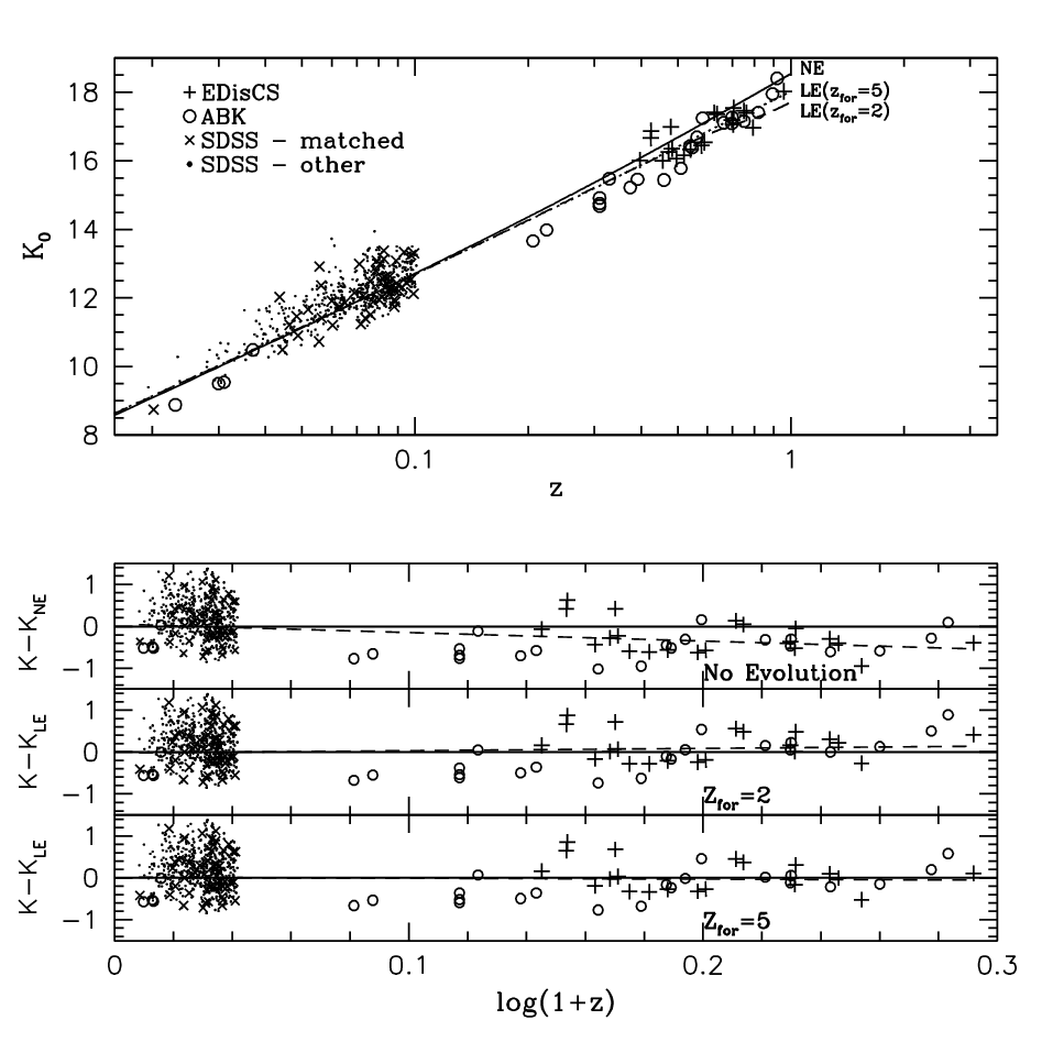
Figure 2 shows the rest-frame -band Hubble diagram for the BCGs in the SDSS/2MASS, EDisCS and ABK clusters. The estimated random uncertainties in the -band magnitudes add little to the scatter of the points, as they are –mag for the EDisCS and ABK BCGs and mag for the SDSS/2MASS BCGs.
| SDSS BCG ID | (km/s)b | |||
|---|---|---|---|---|
| 587726014532550731 | 0.02015 | 8.7 | 502 | |
| 587722953306931328 | 0.04362 | 12.0 | 264 | |
| 588015507664928793 | 0.04437 | 10.5 | 933 | |
| 587728932421042326 | 0.04631 | 11.2 | 556 | |
| 587728670418272398 | 0.04845 | 11.5 | 570 | |
| 588848899917611022 | 0.04876 | 10.9 | 211 | |
| 587729387149852828 | 0.05189 | 11.7 | 547 | |
| 587727227305263139 | 0.05558 | 10.7 | 903 | |
| 587722952231944566 | 0.05566 | 12.9 | 685 | |
| 587734304344178742 | 0.05625 | 12.4 | 915 | |
| 587733081347195107 | 0.05643 | 11.4 | 441 | |
| 587722983377535296 | 0.06003 | 11.9 | 506 | |
| 587729751131029774 | 0.06029 | 11.2 | 512 | |
| 587732134304350396 | 0.06288 | 11.7 | 613 | |
| 587731185668849907 | 0.06517 | 11.9 | 1084 | |
| 588010360151146773 | 0.06901 | 12.2 | 800 | |
| 587733081882755176 | 0.07107 | 13.0 | 543 | |
| 587726032259973170 | 0.07174 | 11.2 | 514 | |
| 587732582591168714 | 0.07267 | 12.1 | 582 | |
| 587735666921898155 | 0.07371 | 11.4 | 670 | |
| 587731680111820927 | 0.07587 | 12.5 | 902 | |
| 587727225689538702 | 0.07618 | 11.5 | 812 | |
| 587726016681476254 | 0.07738 | 11.9 | 966 | |
| 587727212807192844 | 0.07868 | 12.8 | 765 | |
| 587726031184920689 | 0.07919 | 13.1 | 327 | |
| 587725576423342431 | 0.08012 | 12.0 | 1156 | |
| 587726031184330907 | 0.08044 | 13.0 | 677 | |
| 588015508205994134 | 0.08157 | 12.0 | 497 | |
| 587725505559986486 | 0.08182 | 12.6 | 613 | |
| 587730817361641713 | 0.08255 | 13.1 | 406 | |
| 587726877271130340 | 0.08257 | 13.4 | 315 | |
| 587726032776593461 | 0.08316 | 12.6 | 424 | |
| 587733080814780480 | 0.08330 | 12.3 | 625 | |
| 587730816824508498 | 0.08512 | 12.5 | 229 | |
| 587729782810345782 | 0.08578 | 12.3 | 530 | |
| 588013381670994051 | 0.08581 | 12.6 | 409 | |
| 587729752747278348 | 0.08803 | 11.7 | 951 | |
| 587733410986590314 | 0.08804 | 11.9 | 705 | |
| 588848899917873272 | 0.08820 | 12.2 | 1020 | |
| 588848900454678767 | 0.08856 | 11.9 | 708 | |
| 587733604808458243 | 0.08901 | 13.1 | 556 | |
| 587736618787733576 | 0.09010 | 12.4 | 974 | |
| 587722982834438274 | 0.09059 | 12.2 | 748 | |
| 587726100415774941 | 0.09243 | 12.3 | 513 | |
| 587735694836039706 | 0.09356 | 13.3 | 554 | |
| 587727212274057247 | 0.09465 | 12.4 | 513 | |
| 588010359621156952 | 0.09742 | 13.2 | 1074 | |
| 587726032234741909 | 0.09767 | 12.5 | 388 | |
| 587729407545639093 | 0.09903 | 12.1 | 1127 | |
| 587726032245620919 | 0.09947 | 13.3 | 746 |
The solid line in figure 2 is the no-evolution prediction, which takes into account dimming solely due to distance modulus as a function of redshift. The other two lines plotted are passive evolution predictions from the population synthesis models of Bruzual & Charlot (2003), using a Salpeter (1955) initial mass function with solar metallicity. We have assumed a fixed metallicity for the BCGs as the actual metal content and its evolution is unknown. However, ABK showed that changing the metal content makes little difference to the passive luminosity evolution22 2 The metallicity of the BCGs is discussed in section 2.3.. The dashed line in figure 2 shows the predicted evolution of a stellar population which forms at a redshift of 2 and evolves passively thereafter. Similarly, the dotted line is the prediction for a passively evolving stellar system formed at a redshift of 5. The prediction lines are normalised at low- to the mean of the 1000 -matched SDSS/2MASS subsamples. Contrary to the findings of ABK, who found no evidence for luminosity evolution in the -band luminosity of BCGs, figure 2 indicates relatively small, but significant, luminosity evolution: BCGs at appear to be, on average, 1.7 times brighter in the rest-frame band than ones. Indeed, the BCGs follow quite closely the passive luminosity evolution lines, with a scatter of mag. The different behaviour we have found is mainly due to the low- comparison sample used to derive the low- normalisation of the Hubble diagram. Due to the limited amount of -band data for BCGs available at the time, ABK used a small ad-hoc sample of only 4 low-z BCGs. The large uncertainty on the normalisation from such a small sample was exacerbated by the fact that most of these clusters had relatively high velocity dispersions, biasing their magnitudes. This highlights the dangers of comparing low- and high- cluster samples without carefully matching their properties. Indeed, had we used the entire SDSS/2MASS BCGs sample (small dots in Figure 2) to normalise the Hubble diagram, we would have derived a much stronger evolution since the majority of the local clusters have low velocity dispersions and their BCGs are therefore too faint (cf. section 2.4).
The three lower panels of figure 2 show the same data after subtracting the no-evolution and passive-evolution predictions. As mentioned above, it is clear from the top panel that the BCGs show a relatively small, but significant, luminosity evolution over the redshift range plotted. The results of subtracting the passive evolution model predictions from the data are shown in the middle and bottom panels assuming and respectively. The lines of best fit in these panels (derived from the average of the 1000 low- subsamples) are very close to the passive luminosity evolution predictions themselves. This is in agreement with the observed colour evolution of these objects, which suggests that their stars were formed at a redshift and then evolved passively (see section 2.3).
If the stellar populations of these objects are passively evolving, as their colour evolution suggests (section 2.3), the observed luminosity evolution can be used to place limits to the amount of growth in the stellar mass of the BCGs. Following the method of ABK we parameterize the stellar mass evolution as . Least-squares fits to the data points in the bottom panels of figure 2 give the following results:
This means that we do not detect any significant change in the stellar mass of these objects. Our data is compatible with zero growth. Formally, the derived values and their associated errors imply that, if the stellar populations in these galaxies formed at , the stellar mass cannot have grown by more than a factor 1.9 between and (3- upper limit). For , the upper limit reduces to a factor of 1.4 (i.e., only 40%). This contrasts with the results obtained by ABK, who suggested stellar mass growths for the BCGs of factors between 2 and 4 since . As mentioned above, this difference is mainly due to their low- normalisation. We compare the observed mass growth with the results from semi-analytic models in section 3.

Collins & Mann (1998) and Brough et al. (2002) found that the amount of stellar mass growth shown by the BCGs could be dependent on the X-ray luminosity of the host cluster, with BCGs in high X-ray luminosity clusters showing little or no stellar mass growth since , while BCGs in low X-ray luminosity clusters exhibit a large variation in their stellar mass growth, from clusters showing no growth to a few growing by factors of up to . As discussed in §2.4, the cluster X-ray luminosity and velocity dispersion can be taken as a proxies for cluster mass. If we divide our low- and high- cluster samples into two equal subsamples, one with km s-1 and the other with km s-1 we find that the inferred stellar mass growth does not seem to depend on : the stellar mass of the BCGs seems to have remained roughly constant for both subsamples (albeit, with weaker formal limits given the smaller sample sizes). This is shown in figure 3, which presents again the lower panels of figure 2 with the data split into high and low subsamples. There is no significant difference in the luminosity evolution rate of the two subsamples. However, there is clearly an offset between the lines of best fit in each panel of figure 3, with the high- sample being brighter in each case. This implies a significant dependence of the luminosity of the BCG on cluster velocity dispersion, as discussed in section 2.4.
To test whether our conclusions depend strongly on the choice of galaxy evolution models, we have re-calculated the expected passive -band luminosity evolution (cf. figure 2) using the models of Maraston et al. (2006). Since these models use a very different prescription for TP-AGB stars, the near-IR luminosity evolution is significantly different from that of Bruzual & Charlot (2003) for stellar populations with ages –Gyr. However, for the range of ages relevant to our analysis (–Gyr), the model predictions agree within mag for a given metallicity and IMF. We are thus confident that the conclusions of this section are reasonably model-independent.
2.3 Colours
Figure 4 shows the observed-frame and colours for the EDisCS and SDSS/2MASS BCGs, plotted as a function of redshift. For the EDisCS BCGs a radius circular aperture was used to measure the colours. This aperture is large enough to sample a significant fraction of the BCG’s light, while keeping sky-subtraction errors small33 3 Measuring galaxy colours inside the metric aperture used in section 2.2 (average radius) makes no significant difference to the conclusions of this section.. The radius at the average redshift of the EDisCS BCGs, (), corresponds to an aperture of radius at the average redshift of the SDSS BCGs (). Optical and near-infrared photometry for the SDSS/2MASS sample was measured inside circular apertures with radius, and transformed into the system following Blanton & Roweis (2007).
The colours were corrected for galactic extinction but not -corrected. The lines shown in figure 4 are predictions created using the population synthesis code of Bruzual & Charlot (2003). The solid lines represent the expected colour evolution of a stellar population with solar metallicity and a Salpeter (1955) IMF which formed in an instantaneous burst at and then evolved passively. The dotted and dashed lines show the expected evolution for similar stellar populations that formed at and respectively. It is clear from figure 4 that, within the model uncertainties (see below), there is reasonably good agreement between the data and the passive evolution models with and 5. As expected, the model for does not fit the data at all. The agreement between the colours of the BCGs and the passive evolution models is a strong indication that the BCGs are composed of stellar populations that formed at and have been evolving passively since. Similar conclusions are obtained using the Maraston et al. (2006) models. For the range of ages relevant to between 2 and 5, these models predict colours which agree with those of Bruzual & Charlot (2003) within mag. This should be taken as an indication of the typical uncertainties associated with model colours. For that reason, the fact that the BCG colours seem to agree with the models while for there is better agreement with is not significant. Nevertheless, since the band samples the rest-frame ultraviolet, a very small amount of recent star formation (say, % by mass) could easily make the observed colours bluer by while having negligible effect on .
As the metallicity of the BCGs is unknown, the colour evolution predictions were also calculated for a stellar population with approximately double solar metallicity and also approximately half solar metallicity. These predictions were found to lie nowhere near the plotted data points, being far too red and blue respectively to reproduce the colour evolution exhibited by the BCGs. This shows that although the colour evolution predictions are sensitive to changes in metallicity, the assumption of approximately solar metallicity is a reasonable one.

2.4 BCG -band luminosity and cluster velocity dispersion.
Arguably, the most fundamental property of a cluster is its mass, so it is not unreasonable to expect that the luminosity (and stellar mass) of the BCGs may be related to it. Several observational properties can be used as proxies for the cluster mass, including the cluster X-ray luminosity and temperature and the cluster velocity dispersion . Indeed, Edge & Stewart (1991) found a significant correlation, in a low- sample, between the optical luminosity of the BCGs and the X-ray luminosity and temperature of the parent clusters in the sense that hotter and more X-ray bright clusters host brighter BCGs.
Velocity dispersions are available for all the EDisCS and SDSS clusters and 10 of the clusters studied by ABK. Columns 4 of tables 1 and 2 show the velocity dispersions of the EDisCS and SDSS/2MASS -matched cluster samples. A full description of the calculation of the values for the SDSS clusters can be found in von der Linden et al. (2007). Information regarding the EDisCS values can be found in Halliday et al. (2004), Poggianti et al. (2006) and Milvang-Jensen et al. (2008). The velocity dispersions for the ABK clusters are taken from Girardi & Mezzetti (2001) and Lubin et al. (2002). Note that in all these studies the cluster velocity dispersions have been determined following very similar methods, and are thus directly comparable.
In order to test for any relationship between the BCG -band luminosity (or stellar mass) and the cluster mass, we have calculated the residuals around the three lines of best fit shown in the bottom three panels of figure 2 and plotted them against in figure 7. This procedure should correct for redshift-related effects. The panels show, from top to bottom, the residuals around the line of best fit after the rest-frame -band magnitudes have been corrected for no evolution, passive evolution with and passive evolution with , respectively (cf. figure 2). The symbols for the EDisCS and the ABK samples are the same as in figure 2. As an illustration, we also show (crosses) the BCGs in the SDSS/2MASS -matched subsample whose line of best fit (see below) is closest to the mean of the 1000 subsamples.
There is a clear trend in each panel of figure 7 indicating that clusters with large velocity dispersions, and presumably large masses, tend to have brighter BCGs. A Spearman rank correlation coefficient analysis indicates that all these correlations are significant at a level greater than 99.9%.
To explore whether the luminosity- correlation evolves with redshift, we analysed the intermediate-redshift EDisCS/ABK clusters and the low-redshift SDSS ones separately. We define as the rest-frame -band luminosity of the BCGs corrected either assuming no luminosity evolution (N.E.) or passive luminosity evolution for or 5. If we parameterize the trends shown in figure 7 as , simple least-squares fits to the EDisCS/ABK data give
and for the mean of the 1000 SDSS/2MASS -matched cluster subsamples we get in all cases.
Note that the correlations found and their estimated slopes are robust against changes in the way we account for the passive luminosity evolution of the BCGs.
The slopes of the – relations are the same for the low- and high- samples. This seems to indicate that in the the range of redshifts explored here the rate of the BCG buildup and that of the cluster are linked in a way that does not depend strongly on cosmic time.
Another interesting result is that, although significant, the dependency of (presumably proportional to the BCG’s stellar mass ) on is relatively weak. If we assume that the cluster mass is proportional to , where is the radius of a sphere with interior mean density 200 times the critical density of the universe at the cluster redshift. If we also assume that, at a given redshift, (Carlberg et al. 1997; Finn et al. 2005), then , and . Thus, the stellar mass of BCGs changes only by over a two-order-of-magnitude range in cluster mass. This is not surprising: it has long been known that BCG luminosities measured inside fixed metric apertures provide reasonable standard candles almost independent of the cluster richness (Postman & Lauer 1995).
Very recently, Brough et al. (2008) and Stott et al. (2008) have found similar results for X-ray selected cluster samples.
3 Comparison with galaxy formation models

In this section, we compare our empirical results with theoretical predictions from De Lucia & Blaizot (2007). These authors use a combination of large N-body collisionless cosmological simulations and semi-analytic techniques. The semi-analytic models are grafted onto the hierarchical merging trees extracted from the Millennium Simulation (Springel et al., 2005). In this study, we compare our results with two versions of the semi-analytic model which differ for the prescriptions adopted for the supernovae feedback. In the following we will refer as model 1 to a model which employ the same supernovae feedback model used in De Lucia et al. (2006) where the ejection rates are computed on the basis of energy conservation arguments. We will refer as model 2 to a model which adopts the same supernovae feedback model as in Croton et al. (2006) where the ejection rates are proportional to the star formation rate. De Lucia & Blaizot (2007) have shown that model 1 results in a slower evolution of the K-band magnitudes as a function of redshift, albeit producing K-band magnitudes of local BCGs brighter than a factor of about mag with respect to results from model 2.
In order to compare our results to model predictions, we extracted haloes within the simulation box, uniformly distributed in log(mass) between and . We extracted the haloes from the output of the simulation at and followed their history back in time by tracking, at each time, the main progenitor branch defined as in De Lucia & Blaizot (2007). For each SN feedback model, we have then created tables with rest-frame and observed-frame magnitudes in 5 different bands (, , , , , and ) for the brightest galaxy in each halo. For each halo we have also calculated the 3D and projected velocity dispersions using all galaxies within at three redshifts (, , and ). In order to simulate the errors associated with the observed values, for each halo and each redshift we extracted a random number of objects, between and from all galaxies within and computed the 1D velocity dispersion and their confidence limits using the same method that was used to calculate the velocity dispersions for the EDisCS clusters (Halliday et al., 2004)44 4 In the smallest haloes there are cases where the number of objects is less than 20. In these cases we take all objects for the calculation of the velocity dispersion. Note, however, that this situation seldom arises for the final comparison sample, once a minimum velocity dispersion cut is applied (as we do in our analysis).. This method tries to mimic the observational uncertainties in the model predictions.
When selecting the model cluster sample to compare with observations, there are two obvious alternatives. First, one could follow the evolution of the same model clusters, i.e., select clusters at all redshifts which, at a given redshift (e.g., ), have . Second, one could follow similar cluster “samples”, i.e., select clusters that, at each redshift, have . Obviously, the first selection tells us what happens to the same set of galaxies, while the second one is probably closer to observations since it follows comparable samples. We will therefore follow the second selection method with km s-1 (64–70 model clusters, depending on redshift) and km s-1 (28–45 model clusters, also depending on redshift), which seem reasonable limits for comparison with our dataset (cf. figure 1). Note that the for EDisCS is not well defined since velocity dispersion was not explicitly part of the EDisCS cluster selection criteria. However, since the results do not depend on the precise value of this limit, the choice is not critical.
Figure 5 shows the model distribution at each redshift bin obtained using this selection technique. Although the model values were not explicitly matched in each redshift bin, as was done for the observational data, their distributions are well matched at all redshifts considered. Moreover, they are also well matched to the values of the observational data (c.f. figure 1)

The first result of the comparison is that the colours of the model galaxies are similar to the observed ones for model 1, i.e., close to those of passively-evolving stellar populations formed early. This suggests that even if the buildup of the galaxies’ stellar mass is gradual, this growth is dominated by the accretion of old stellar populations rather than by new star formation. Model 2 predicts somewhat bluer colours.
Both models 1 and 2 predict a growth in stellar mass that is significantly stronger than observed: the stellar mass of model BCGs grows by about a factor of – between and , while the observations are compatible with no growth at all and seem to rule out a factor of two growth since (cf. section 2.2). The stellar mass growth in the models does not depend strongly on which feedback method is used, although it is marginally stronger in model 2. The stellar mass growth is also quite insensitive to the value of , which agrees with the observed independence of the stellar mass growth on . These results are illustrated in figure 6.
Finally, we compare the observed dependency of the BCGs’ corrected -band luminosity (or stellar mass) with the cluster velocity dispersion (cf. section 2.4). For model 1, regardless of the exact value of , the models predict, at all the redshifts considered, or . Model 2 predicts or . The data suggest a much weaker dependency of the stellar mass on the cluster velocity dispersion or mass. That is clearly shown in figure 7: the dashed line represents the average slope from the model predictions, which is significantly steeper than the data.
One major caveat in the comparison of our observations with the semi-analytical model results is that we have used magnitudes measured inside a fixed metric aperture while the models compute total magnitudes. Observationally it is very difficult (virtually impossible) to measure accurate total magnitudes for the BCGs (see, e.g., Gonzalez et al. 2005). Indeed, it is not even clear whether one should include the intracluster light (ICL) as part of the BCG’s luminosity (Gonzalez et al. 2007). A kpc diameter aperture encompasses only 25%–50% of the total light contained in the BCG and ICL (Gonzalez, Zaritsky and Zabludoff, private communication). Interestingly, using the -band data published by these authors we find that although their kpc aperture magnitudes show a dependency with compatible with our measurements, their total BCG+ICL luminosities show a significantly steeper dependence (). Although the slope is still considerably shallower than the model predictions, this could explain at least part of the disagreement between models and observations. Note, however, that the scatter is large and their sample relatively small.
On the other hand, the models do not have spatial information regarding the distribution of the BCG light, so aperture magnitudes cannot be calculated. It is also not clear whether the luminosities of the model BCGs contain some of what, observationally, we could call intracluster light. The luminosity of the model BCG includes the stars formed in the central cluster halo and the stars formed in galaxies that merged with the central galaxy, but not stars stripped from other cluster galaxies due to tidal and “harassment” effects, since these are not modeled. Therefore, any discrepancy (and/or agreement) found in the behaviour of the observed and model BCGs should be taken with caution, since not all the physical effects which potentially contribute to the growth of the BCGs are taken into account.
A possible way of reconciling our observations and the model predictions could be that, if there is a large stellar mass growth in BCGs (e.g., a factor of 4 since ), these stars could lie outside of the kpc apertures we have used in our measurements. In that case, such a growth would really represent the growth of the intracluster component rather than the central BCG. How such growth would depend on the cluster properties is difficult to predict, but it is clear that the intracluster component could play a very important rôle in the formation and evolution of clusters (see, e.g., Lin & Mohr 2004). For recent theoretical studies of the formation of the intracluster light, see Monaco et al. (2006) and Conroy et al. (2007).

4 Conclusions
In this paper we present new -band data for 21 brightest cluster galaxies (BCGs) from the ESO Distant Cluster Survey (EDisCS). Combining these data with the photometry published by Aragón-Salamanca, Baugh & Kauffmann (1998) we have built a sample of 42 BCGs with good quality near-infrared photometry in the redshift range. We have also put together a low-redshift () comparison sample from the BCG catalogue of von der Linden et al. (2007) for which optical and near-infrared photometry is available from the SDSS and 2MASS. By comparing the properties of the BCGs in the low- and high- datasets and those of their parent clusters we have carried out a detailed study of the evolution of these galaxies. Since, as we demonstrate, the properties of the BCGs depend upon the velocity dispersion (and thus presumably the mass) of the cluster they inhabit, we carefully match the distributions of our samples before comparing them. In this work the luminosities of the BCGs are measured inside a fixed metric circular aperture with kpc diameter. The main conclusions of our study are:
- 1.
In agreement with previous studies, we find that the -band Hubble diagram for BCGs exhibits very low scatter (mag) over a redshift range of .
- 2.
The colour evolution of BCGs as a function of redshift shows good agreement with population synthesis models of stellar populations that formed at and evolved passively thereafter.
- 3.
In contrast with some previous studies (e.g., Aragón-Salamanca et al. 1998) we find that the rest-frame -band luminosity evolution of the BCGs is also well reproduced by passive evolution models. The main reason for this discrepancy is the use of a different, hopefully more accurate, low redshift comparison sample with well-matched distribution.
- 4.
The agreement of the observations with passive luminosity evolution models means that we do not detect any significant change in the stellar mass of the BCG since . Formally, we rule out a growth in the stellar mass larger than a factor of 1.9 between and (3- upper limit). This result does not seem to depend on the velocity dispersion of the parent cluster.
- 5.
We find that there is a correlation between (the 1D velocity dispersion of the clusters) and the -band luminosity of the BCGs (after correcting for passive evolution). Clusters with large velocity dispersions, and therefore masses, tend to have brighter BCGs, i.e., BCGs with larger stellar masses. This dependency, although significant, is relatively weak: the stellar mass of the BCGs changes only by over a two-order-of-magnitude range in cluster mass. Furthermore, this dependency doesn’t change significantly with redshift.
We have compared our observational results with the hierarchical galaxy formation and evolution model predictions of De Lucia & Blaizot (2007). One major difficulty in this comparison is that we have measured magnitudes inside a fixed metric aperture while the models compute total luminosities. We find that the models predict colours which are in reasonable agreement with the observations because the growth in stellar mass is dominated by the accretion of old stars. However, the stellar mass in the model BCGs grows by a factor of – since , a growth rate which seems to be ruled out by the observations. The models predict a dependency between the BCG’s stellar mass and the velocity dispersion (mass) of the parent cluster in the same sense as the data, but the dependency is significantly stronger than observed. It therefore seems as if building realistic BCGs is another challenge for this kind of models, indicating that the underlying physics is far from being completely understood.
Acknowledgments
This paper is partly based on observations collected at the European Southern Observatory, Chile, as part of large programme 166.A–0162 (the ESO Distant Cluster Survey). This publication makes use of data products from the Two Micron All Sky Survey, which is a joint project of the University of Massachusetts and the Infrared Processing and Analysis Center/California Institute of Technology, funded by the National Aeronautics and Space Administration and the National Science Foundation. IW and AAS acknowledge financial support from PPARC. The Dark Cosmology Centre is funded by the Danish National Research Foundation.
This publication makes use of data products from the Sloan Digital Sky Survey (SDSS). Funding for the SDSS and SDSS-II has been provided by the Alfred P. Sloan Foundation, the Participating Institutions, the National Science Foundation, the U.S. Department of Energy, the National Aeronautics and Space Administration, the Japanese Monbukagakusho, the Max Planck Society, and the Higher Education Funding Council for England. The SDSS Web Site is http://www.sdss.org/.
The SDSS is managed by the Astrophysical Research Consortium for the Participating Institutions. The Participating Institutions are the American Museum of Natural History, Astrophysical Institute Potsdam, University of Basel, University of Cambridge, Case Western Reserve University, University of Chicago, Drexel University, Fermilab, the Institute for Advanced Study, the Japan Participation Group, Johns Hopkins University, the Joint Institute for Nuclear Astrophysics, the Kavli Institute for Particle Astrophysics and Cosmology, the Korean Scientist Group, the Chinese Academy of Sciences (LAMOST), Los Alamos National Laboratory, the Max-Planck-Institute for Astronomy (MPIA), the Max-Planck-Institute for Astrophysics (MPA), New Mexico State University, Ohio State University, University of Pittsburgh, University of Portsmouth, Princeton University, the United States Naval Observatory, and the University of Washington.
References
- Aragón-Salamanca et al. (1998) Aragón-Salamanca A., Baugh C. M., Kauffmann G., 1998, MNRAS, 297, 427
- Bernstein & Bhavsar (2001) Bernstein J. P., Bhavsar S. P., 2001, MNRAS, 322, 625
- Blanton & Roweis (2007) Blanton M. R., Roweis S., 2007, AJ, 133, 734
- Brough et al. (2002) Brough S., Collins C. A., Burke D. J., Mann R. G., Lynam P. D., 2002, MNRAS, 329, L53+
- Brough et al. (2008) Brough S., Couch W. J., Collins C. A., Jarrett T., Burke D. J., Mann R. G., 2008, MNRAS, pp L16+
- Bruzual & Charlot (2003) Bruzual G., Charlot S., 2003, MNRAS, 344, 1000
- Carlberg et al. (1997) Carlberg R. G., Yee H. K. C., Ellingson E., 1997, ApJ, 478, 462
- Collins & Mann (1998) Collins C. A., Mann R. G., 1998, MNRAS, 297, 128
- Conroy et al. (2007) Conroy C., Wechsler R. H., Kravtsov A. V., 2007, ApJ, 668, 826
- Croton et al. (2006) Croton D. J., et al., 2006, MNRAS, 365, 11
- De Lucia & Blaizot (2007) De Lucia G., Blaizot J., 2007, MNRAS, 375, 2
- De Lucia et al. (2006) De Lucia G., Springel V., White S. D. M., Croton D., Kauffmann G., 2006, MNRAS, 366, 499
- Dressler (1978) Dressler A., 1978, ApJ, 223, 765
- Edge & Stewart (1991) Edge A. C., Stewart G. C., 1991, MNRAS, 252, 428
- Finn et al. (2005) Finn R. A., et al., 2005, ApJ, 630, 206
- Girardi & Mezzetti (2001) Girardi M., Mezzetti M., 2001, ApJ, 548, 79
- Gonzalez et al. (2005) Gonzalez A. H., Zabludoff A. I., Zaritsky D., 2005, ApJ, 618, 195
- Gonzalez et al. (2001) Gonzalez A. H., Zaritsky D., Dalcanton J. J., Nelson A., 2001, ApJS, 137, 117
- Gonzalez et al. (2002) Gonzalez A. H., Zaritsky D., Simard L., Clowe D., White S. D. M., 2002, ApJ, 579, 577
- Gonzalez et al. (2007) Gonzalez A. H., Zaritsky D., Zabludoff A. I., 2007, ApJ, 666, 147
- Gunn & Oke (1975) Gunn J. E., Oke J. B., 1975, ApJ, 195, 255
- Halliday et al. (2004) Halliday C., et al., 2004, A&A, 427, 397
- Hoessel et al. (1980) Hoessel J. G., Gunn J. E., Thuan T. X., 1980, ApJ, 241, 486
- Humason et al. (1956) Humason M. L., Mayall N. U., Sandage A. R., 1956, AJ, 61, 97
- Lauer & Postman (1992) Lauer T. R., Postman M., 1992, ApJ, 400, L47
- Lin & Mohr (2004) Lin Y.-T., Mohr J. J., 2004, ApJ, 617, 879
- Lubin et al. (2002) Lubin L. M., Oke J. B., Postman M., 2002, AJ, 124, 1905
- Mannucci et al. (2001) Mannucci F., Basile F., Poggianti B. M., Cimatti A., Daddi E., Pozzetti L., Vanzi L., 2001, MNRAS, 326, 745
- Maraston et al. (2006) Maraston C., Daddi E., Renzini A., Cimatti A., Dickinson M., Papovich C., Pasquali A., Pirzkal N., 2006, ApJ, 652, 85
- Miller et al. (2005) Miller C. J., et al., 2005, AJ, 130, 968
- Milvang-Jensen et al. (2008) Milvang-Jensen B., et al., 2008, A&A, in press, arXiv:0802.0149
- Monaco et al. (2006) Monaco P., Murante G., Borgani S., Fontanot F., 2006, ApJ, 652, L89
- Nelson et al. (2002) Nelson A. E., Simard L., Zaritsky D., Dalcanton J. J., Gonzalez A. H., 2002, ApJ, 567, 144
- Oegerle & Hoessel (1991) Oegerle W. R., Hoessel J. G., 1991, ApJ, 375, 15
- Poggianti et al. (2006) Poggianti B. M., et al., 2006, ApJ, 642, 188
- Postman & Lauer (1995) Postman M., Lauer T. R., 1995, ApJ, 440, 28
- Salpeter (1955) Salpeter E. E., 1955, ApJ, 121, 161
- Sandage (1972) Sandage A., 1972, ApJ, 178, 1
- Sandage (1976) Sandage A., 1976, ApJ, 205, 6
- Sandage (1988) Sandage A., 1988, ARA&A, 26, 561
- Sandage & Hardy (1973) Sandage A., Hardy E., 1973, ApJ, 183, 743
- Schlegel et al. (1998) Schlegel D. J., Finkbeiner D. P., Davis M., 1998, ApJ, 500, 525
- Schneider et al. (1983) Schneider D. P., Gunn J. E., Hoessel J. G., 1983, ApJ, 264, 337
- Skrutskie et al. (2006) Skrutskie M. F., et al., 2006, AJ, 131, 1163
- Spergel et al. (2003) Spergel D. N., et al., 2003, ApJS, 148, 175
- Springel et al. (2005) Springel V., et al., 2005, Nature, 435, 629
- Stott et al. (2008) Stott J. P., Edge A. C., Smith G. P., Swinbank A. M., Ebeling H., 2008, MNRAS, 384, 1502
- Stoughton et al. (2002) Stoughton C., et al., 2002, AJ, 123, 485
- von der Linden et al. (2007) von der Linden A., Best P. N., Kauffmann G., White S. D. M., 2007, MNRAS, pp 578–+
- White et al. (2005) White S. D. M., et al., 2005, A&A, 444, 365
- York et al. (2000) York D. G., et al., 2000, AJ, 120, 1579