BINARY OW GEMINORUM
A. Majcher1,3, J. Ł. Janowski1 and M. Cikała1,4
1Uniwersytet Mikołaja Kopernika, Centrum Astronomii, Toruń, Polska
2 National Astronomical Observatory Rozhen, Institute of Astronomy, Smolyan, Bulgaria
3 Instytut Problemów Ja̧drowych im. Andrzeja Sołtana Otwock – Świerk, Warszawa, Polska
4 Obserwatorium Astronomiczne im. T. Banachiewicza, Wȩglówka, Polska
Introduction.
OW Gem is an unusual, long-period eclipsing binary, composed of two evolved supergiant stars. Variability
of the star has been noticed by Kaiser1 during photographic searches of nova stars in March 1988.
Photoelectric observation soon showed a shallow secondary minimum2 at phase 0.23 in the V band,
indicating that the orbit has high eccentricity. It turned out that eclipses were visible on Harvard photographic
plates3 already from 1902. The orbital period (1258.59 days - about 3.45 years) was derived from 11 eclipse
events, which took place before 19924. Radial velocity data of very good quality were obtained
by Griffin Duquennoy5 (in tables: GD), and used by them for the first reliable analysis of the system.
The presence of eclipses distinguish OW Gem from several known similar systems6, hence we know the exact masses
of the components in this case ( and ). The object has turned out to be unusually
interesting. Both its components have quite large, but considerably different masses and they are now
simultaneously in the short phase of supergiant evolution. Therefore, the evolutionary status of the system
seems to be in contradiction to the current stellar evolutionary models.
Many attempts of modelling the system parameters appeared in recent years as a result of several authors
carrying out good quality multicolour photometric measurements of the eclipses. Derekas et al.7 have
presented a simple model based on observations of the main minimum at the turn of the years 2001 and 2002, in
which they estimate the temperature and the luminosity of the components. Another group (Terrell et al.8) has
used Wilson – Devinney code (hereafter: WD) for modelling and operating on Kaiser et al.9 photoelectric
observational data together with the only available at that time radial velocity measurements5, and they have
obtained a complete set of parameters. In the same year, we presented a simple model10 within the confines
of which we have obtained the inclination of the orbit and the most probable temperature of the
secondary (cool) component for an assumed value of the primary temperature . In that model, the
limb darkening was neglected and stellar fluxes were approximated as blackbodies. This work presents new
multicolour photometry covering one (1995) primary eclipse and three (1995, 2002, 2006) secondary eclipses.
We have independently obtained a complete set of parameters using our own and part of Derekas et al.7
photometric data. The new - partly not published earlier - radial velocity data (Appendix – Table 12)
were used, due to kindness of Roger Griffin which has collected them together with A. Duquennoy during the last
fourteen years. Suggested by Dr R.F. Griffin weight were applied. Additionally three our own radial velocity
measurements (Appendix – Table 13) were included for analysis.
Observational photometric data
An international observational campaign was organized by Terrell et al. during 1995 primary and secondary eclipses11. Responding to this, we obtained multicolour photometry for both events with a 60 cm Cassegrain reflector at Piwnice Observatory near Toruń (Poland). We used a single-channel diaphragm photometer with non – cooled EMI 9558B photomultiplier. Our response curves for U, B and V bands were very close to the standard Johnson’s system, whereas our broad R, I bands had significantly shorter mean wavelengths than Johnson RI and Cousins (RI)C (Table 1). The accuracy of our measurements was , , , and in UBVRI respectively. Unfortunately, in the analysis based on the 1995 campaign9 our photometric data were not included. Our observations of the 1995 secondary eclipse have poor time covering as a result of bad weather. To fill the gaps in the light curves, new data were obtained nearby and during the 2002 secondary eclipse. A single–channel diaphragm photometer, with a cooled Burle C31034 photomultiplier and a set of five filters U, B, V, RC, IC were used. Their response curves were close to the standard Johnson–Cousins UBV(RI)C system (Table 1). Additionally, two intermediate–band interference filters (), (located at around ) and (located in the continuum around ) were used. The accuracy of these measurements was , , , and in UBVRCIC respectively. Data around the last 2006 secondary minimum have been obtained with two new CCD detectors (SBIG: STL 11000 and STL 1001) with new filters set. The mean wavelength of these photometric systems are presented and compared with the two previous photometric systems in Table 1. The accuracy was , , , and in UBVRCIC filters respectively. HD 258848 was chosen as a comparison star and GSC 1332:0578 as a check star, both suggested by Terrell et al.11. Our original differential magnitudes () are presented in the Appendix (Tables 8,9, 10,11), and as UBVRI light curves in Figure 1.
| receiver: | EMI 9558B | Burle C31034 | SBIG:STL 11000 | SBIG:STL 1001 |
|---|---|---|---|---|
| band | ||||
| U | 3708 | 3678 | 3676 | 3600 |
| B | 4342 | 4467 | 4392 | 4400 |
| V | 5436 | 5426 | 5343 | 5404 |
| R | 6391 | 6689 | 6319 | 6414 |
| I | 7420 | 8380 | 8020 | 8305 |
Period analysis
The O-C analysis was carried out for verification of the orbital period and for determination of the time between primary and secondary minima. The times of minima from our obserwations and the time of the secondary minimum from Williams2 were obtained using Kwee and Van Woerden method12. The times of collected minima are presented in Table 2. The moment of primary minimum with was excluded from the analysis because of its obviously high error. The values of O-C residuals for the primary events were calculated from Williams Kaiser’s4 ephemeris:
| (1) |
and are shown in Figure 2. The best fit to these data gives the new ephemeris:
| (2) |
| E | JD-2400000 | error | O-C | Author | Ref | ||
| Primary | |||||||
| – | Kaiser | 4 | |||||
| – | ” | 4 | |||||
| – | ” | 4 | |||||
| – | ” | 4 | |||||
| – | ” | 4 | |||||
| – | ” | 4 | |||||
| – | Fuhrmann | 4 | |||||
| – | ” | 4 | |||||
| – | ” | 4 | |||||
| Kaiser et al. | 4 | ||||||
| Williams Kaiser | 4 | ||||||
| Hager | 13 | ||||||
| this work | – | ||||||
| Kaiser et al. | 9 | ||||||
| Kaiser et al. | 9 | ||||||
| 52 | Derekas et al. | 7 | |||||
| Secondary | |||||||
| 25 | Williams | 2 | |||||
| 27 | this work | – | |||||
| 27 | Kaiser et al. | 9 | |||||
| 29 | Kaiser et al. | 9 | |||||
| 29 | this work | – | |||||
| 30 | this work | – | |||||
| - excluded from our analysis | |||||||
The values O-C for the secondary minima were calculated assuming a new period P=1258.58 days
(Equation 2) and taking into acconut an initial value of the phase shift
according to Williams2 which corresponds to 289.473 days (Figure 2). The residuals obtained
for the six measured secondary minima give a mean value =3.25 0.19 days and hence
the new phase shift is .
Preparation of photometric data
We have used five sets of photometric data for modelling. Four sets were obtained in Piwnice Observatory, two with photomultiplier detectors and two with CCDs. The fifth set of CCD data were obtained by Derekas et al.7. They reported a possible existence of asymmetry in the light curve of the primary eclipse. This effect is not visible in any other data. It seems to be an artefact. Figure 1 in Derekas et al.7 paper shows that all of the VRCIC Szeged Observatory data points lie somewhat above the fit to Piszkéstetö Observatory data points. Because of this we used only Piszkéstetö data to improve the primary eclipse time covering. As a consequence we have collected data from five different photometric systems, which are somewhat shifted in magnitude. Additionally, the depth of minima in particular bands depends on their mean wavelengths. The correction for the depth of secondary eclipse is very small in respect to primary eclipse. To transform the data to the homogenous systems without correction for depth of primary eclipse, we shifted the BVRC Piszkéstetö CCD data (the star GSC 1332-0578 was the comparison star for this data), and UBVR Toruń data obtained with Burle C31034 photomultiplier and STL CCDs to the data obtained in 1995 with EMI 9558B photomultiplier (Table 1). The I passband established by EMI 9558B photomultiplier differs considerably from both Johnsons I and Cousins IC, so the I passband data obtained in the region of phase of primary eclipse were excluded from analysis. The I passband established by STL 1001 CCD detector is quite close to the Cousins IC passband, so this system was adopted as the reference system for the infrared domain. The magnitudes from transformed systems were shifted on reference systems by values presented in Table 3.
| Ref.syst. | Ref.syst. | ||||||
|---|---|---|---|---|---|---|---|
| EMI9558B | STL1001 | ||||||
| Trans.syst. | |||||||
| EMI9558B | – | – | – | – | |||
| Burle C31034 | |||||||
| STL 11000 | |||||||
| STL 1001 | – | ||||||
| Piszkéstetö | – | – | |||||
Additionally, the depths of the secondary minima in transformed systems were corrected on reference systems according to expresion:
| (3) |
where individual values of measured brightnesses are denoted by , mean brightnesses outside of eclipses by (see Table 4), and the parameter is ratio of the depth minimum in reference systems to the depth minimum in transformed systems (see Table 5).
| EMI9558B | |||||
|---|---|---|---|---|---|
| Burle C31034 | |||||
| STL 11000 | |||||
| STL 1001 |
Values of the parameter were
obtained by fitting a 2nd order polynomial to the observational depths of the
secondary eclipse data obtained with the Burle C31034 photomultiplier. All the brightnesses were normalized
to unity corresponding to the mean magnitudes outside the eclipse (Table 4) as it is needed by
the differential correction (DC) procedure of the Wilson – Devinney code.
Modelling the system parameters - methods of solution
We have calculated a simultaneous solution to the photometric data described above and the velocity curves. We have used both the DC and light and velocity curve (LC) programs of the 2003 version of the Wilson – Devinney code14,15, where the radiative functions used are based on Kurucz’s stellar atmosphere models. This allows us to model giants or supergiants in addition to main sequence stars. So, the use of this version of the WD program is more suitable in the OW Gem case. On the other hand in the 2003 version the previous effective wavelength characterization of the bandpasses was replaced by integration over the actual bandpasses of the standard photometric systems. Twenty five standard bands are available in the code. Five of our bands UBVRI used in the analyses adjust well for the UBVRCIC standard bands defined in the program. Unfortunately, our h,c bands do not have equivalents among the standard ones, so we decided to omit them in our analyses.
The Levenberg – Marquardt’s algorithm used in the 2003 version of the WD program together with a
properly selected value of the parameter (see e.g. Kallrath Milone16; Kallrath et al.17)
usually allows finding a solution in the parameter space even when a large group of free parameters for
simultaneous iterations is used. However, the OW Gem orbit is characterized by strong eccentricity which
amplified correlations between the parameters. We have used the method of multiple subsets (MMS) recommended
by Wilson Bierman18 for dealing with this problem. The method relies on disposing the strongest
correlation through separation of the most correlated parameters into different groups. In our case the groups
have included two (seldom three) weakly correlated parameters. The use of the method does not significantly
extend the time of calculation, but a problem appears in the form of unrealistically small values of the
errors. We have received more plausible values of errors by executing additional iterations with all the free
parameters simultaneously. The solution was calculated with the aid of a program we wrote for ”semiautomatic”
iteration, which made it possible to keep control over the result of each iteration by visual inspection of the
evolution of parameters, errors and residuals on the computer screen as a function of the iteration number.
The criterion for a proper solution was set as obtaining the minimum sum of squared residuals over the domain
of parameter space as well as (in some cases) visual inspections of the shape of the surface.
Fixed parameters
OW Gem photometric behaviour does not indicate the possibility of the occurrence of spots on the component’s
surface, so the system was treated as not spotted. Synchronous rotation has been assumed. It is impossible to
find out the temperatures of both the components in OW Gem case using only the WD code, so the temperature
of the hot component was fixed at according to the classification5. The values of
both stars’ temperatures are below , which is a theoretical upper threshold for convective envelopes.
Such cases are characterized by the theoretical values of a bolometric albedo and the exponent in
the bolometric gravity brightening (Lucy19). The third light contribution has been neglected.
The derivatives of the orbital period and were assumed to be equal to zero. A nonlinear, logarithmic
limb darkening law was used. The theoretical coefficients x,y have been calculated according to
the Van Hamme20 tables for: , , log , log .
The free parameters’ initial values
The initial values of , and
have been adopted from Griffin Duquennoy5. The values of the surface linear potentials of the stars
were initially estimated as , from the value of the radius ,
, and mass ratio. A temperature and an inclination have been
taken from our simple model10. The large orbital eccentricity enables to estimation of the parameters
and when we have information about the time separation of the eclipses and about the duration of the
phenomena. From there we have found the initial values of and using formulae
4.4.60 and 4.4.61 from Kallrath Milone16. The parameter was treated differently. This parameter
is connected with manner of orbit solution and it is only formal parameter of WD code, where for circular orbits
phase of periastron is equal to 0.0 for by definition. If we want to get actual value of
periastron phase with WD code for eccentric orbit we have to take into account the value of phase correction .
This parameter can be briefly defined as difference of actual periastron phase for eccentric orbit and periastron
phase that would be for circular orbit with adopted the same periastron longitude .
Three parameters: eccentricity , periastron longitude and parameter are each other dependent.
For that reason parameter can not be treated directly as the other free parameters, but it have to be
searched through the wide area of this parameter’s space in order to find the global minimum and not to land in
a local one.
The orbital geometry solution
The solution was carried out in two basic steps. Both stages of calculations were carried out for many values of parameter according to described below procedure. The first stage aimed to determine the geometry of the orbit through estimation of the parameters: , , , , and . The bandpass luminosity of the primary component is defined in details in the manual of the 2003 version of the WD program. The changes in two parameters, the argument of the periastron and the eccentricity , have a strong influence on the light curves as well as on the velocity curves. The duration of both eclipses and their phase shift depend very strongly on the variations of these two parameters. This timing puts a strong limitation on the values and . The WD program enables solving both velocity curves and many light curves simultaneously21. This advantage of WD code has been used in the first part of the first stage, where the values of the parameters , , were corrected. When a convergence was achieved, then in the second part of the first stage, the parameters , , , which depend only on velocity curves were corrected, then both steps were repeated. The second stage had the purpose of determining first of all the orbital inclination together with the other parameters depending only on the light curves: , , , . and are linear functions of the true potentials on the equipotential surfaces of the stars14. A black–body approximation was used. In order to make the geometric solutions independent of the input values of the radii and the inclination, the first stage of the solution (searching for , , , , ) has been repeated again. A further repeating of both stages did not show changes in the errors limits, so it was considered that for the current value of parameter the final solution for the orbital parameters has been achieved. Each value of parameter relate to one value of sum of weighted squared residuals (), which constitute the quality of obtained fit. The second order polynomial was fitted for function and the minimum of the function was found (Figure 3). This way the final set of orbital parameters has been found and these values are compared with previous solutions in Table 6. The radial velocity curves computed from our parameters (Figure 4) differ slightly from those published earlier by Griffin Duquennoy5 and Terrell et al.8. A good timing of both minima gives better values for and in comparison to previous solutions. However, these parameters force small changes in , and in comparison to the free fitting.
| This work | Griffin 2007⋆⋆ | Terrell et al.8 | GD5 | unit | |
| day | |||||
| – | degree | ||||
| – | |||||
| – | |||||
| degree | |||||
| – | – | – | |||
| – | |||||
| ⋆ | day | ||||
| - The differences between the observed and calculated phase shift of the secondary eclipse | |||||
| - Private communication | |||||
The final solution must give a formally larger standard deviation of the observational points than a free fitting to the radial velocities only, without any timing constraints. This is in contradiction to the Terrell et al.8 solution, who obtained unrealistically low errors for and , as commented by Griffin22. Moreover, a detailed inspection
of ”Figure 1” in Terrell et al.8 shows, that almost all the points which
lie on the descending branch of the secondary minimum are above their synthetic light curves while, the points
which lie on the ascending branch are located below their model. This disagreement in the timing has been
previously noted by Griffin22. Values and parameters obtained by Terrell et al.8
differ significantly from the others results and we have found that their solutions must landed in the local minimum
as a consequence of use incorrect value. Values and parameters which Griffin (2007, private
communication) has obtained with his own, new radial velocity (Appendix – Table 12) are close and almost
consistent in borders of errors to our values. However, becuse of lack of photometry in those solution it is not proper
pair of values, and such and parameters can not give a good timing of the secondary minimum.
The differences between the observed phase shift of the secondary eclipse and that derived
from the orbital solution (Table 6) are hours for our solution, hours for Terrell
et al.8 and minus a few days for orbital parameters carried out from radial velocity only. Taking into
account that we have obtained such a good timing from our analysis, we hope that our parameters are close to the
true ones with realistic errors.
System components physical parameters solution
Knowledge about the orbital geometry allows us to proceed with a part of the modelling leading to exact information about the physical parameters of the components, i.e. temperatures, radii, masses, luminosities. At this stage of the solution a stellar atmospheres approach has replaced the previous black-body approximation. The temperature of the hot component have to be adopted. It is not possible to determine temperature of the both OW Gem components if we do not have at disposal very good quality photometry (accuracy better than ) of both eclipses reaching deep UV and far infrared domain. We have not, and we can obtain temperatures ratio only. The Griffin Duquennoy5 have classified the hot component spectral class as , that according to Straižys Kuriliene23 spectral class - effective temperature classification gives value of temperature . This value of hot component temperture was adopted in our calculations, the same as in other papers. However, we have compared of the OW Gem spectrum with spectra of neighbour class standards, and we have found that the accuracy of this classification is of the order of one subclass. By interpolations with Straižys Kuriliene23 spectral class - effective temperature classification we have estimated uncertainity for temperature of hot component and for corresponding temperature of cold component via temperature ratio as (see table 7). The error of our value given in table 7 it is error of fit to observational data and not the error of parameter determination.
The orbital inclination and radius of the primary component have been found by a search of the ”whole”
surface for their possible values. The method relies on the execution of many fits where the two wanted
parameters are fixed and they are changed in the next runs with the assigned resolution. Such a map of the
function usually allows to find a global minimum, and so proper values of the parameters. The surface
has been obtained by calculating a grid of values of (Figure 5),
for which a 3th order polynomial was fitted. Later on, the minimum of the function was found.
In this way, the inclination and the radius of primary component have been determined, and respondent
the values of the radius of secondary componenet , temperature T2 and the luminosity L1.
The resulted value of the inclination is shown in the Table 6. Table 7 presents our physical
parameters in comparison to those of other authors. Figure 6 demonstrates the quality of the fit to
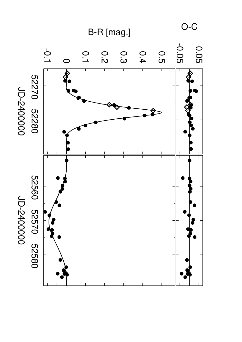
U and V light curves, and Figure 7 demonstrates the variations in the B-R color
index during the primary and the secondary eclipses of OW Gem.
| This work | Terrell et al.8 | GD5 | unit | |
| – | – | |||
| – | – | |||
| – | ||||
| – | ||||
| – | ||||
| – | – | |||
| – | – | |||
| - adopted | ||||
OW Gem spectrum
We used the coude-spectrograph of the 2m RCC telescope at the Rozhen Observatory (Bulgaria) to obtain spectra of OW Gem, with a resolving power R15000, on January 20, 2005 ( 0.88) and April 14, 2006 ( 0.24). The spectral regions covered were 6620-6825 and 6470-6820 respectively. In Figure 8 the spectra of OW Gem are compared with spectra of HD 164136 (), HD 75276 () and HD 159532 (). The spectrum of HD 164136 ( Her) is from the Indo-U.S. library of coudé feed stellar spectra (Valdes et al.24) and the spectra of HD 75276 and HD 159532 are from the UVES library of high-resolution spectra (Bagnulo et al.25). Additionally, a spectrum of the possible merger V838 Mon (Tylenda Soker26, and references therein), obtained at the Rozhen Observatory with the same resolution as the OW Gem spectra, is shown in Figure 8 as well.
In the both spectra the radial velocities were measured (Table 13). In the spectrum on April 14, 2006, obtained during the secondary eclipse, we measured the radial velocity of the primary component only.
Griffin Duquennoy5 classified the primary component of OW Gem as an star. We do not have enough spectral observations and intention to make a detailed spectral classification of both components. However, in Figure 8 it is obvious that the lines in the OW Gem spectrum on April 14, 2006 dominated by the primary component are very similar to the ones in the spectrum of HD 75276. The most remarkable difference between the spectrum of the OW Gem primary and the spectra of Her (noted by Griffin Duquennoy5) and HD 159532 is the rotational velocity which is for Her and for HD 159532 (Snow et al.27). Based on the January 20, 2005 spectrum only, we cannot say anything about the secondary companion spectral class.
The above spectral regions were chosen with the aim of checking up the presence of a weak Li I 6708 line in the spectrum of the secondary component suggested by Griffin Duquennoy5. These authors measured an equivalent width of about or for this lithium line in the composite spectrum. Our April 14, 2006 spectrum (just during the secondary eclipse) is dominated by the primary component. If the lithium line is present then it should be detectable in the January 20, 2005 spectrum (about 5 months before the primary eclipse) in which most of the absorptions are double because of the blending of both component lines. The quality of our spectra is good enough to identify and measure such weak absorptions. As can be seen in Figure 8, in both spectra there are several faint features with equivalent widths of the order of 10-15 in the vicinity of the lithium line. On one hand, none of these faint features disappear in the spectrum on April 14, 2006, as we would expect if the weak lithium line were present only in the secondary spectrum. On the other hand, the radial velocity measurements show that all of these faint features are far from the expected lithium line position for both stars. Therefore, we cannot confirm the presence of the Li I 6708 absorption line, neither in the primary component spectrum nor in the secondary component spectrum.
To explain the unusual evolutionary status of the components, Eggleton28 suggested that OW Gem is a
former triple star in which the F supergiant is a merged remnant of a close sub-binary. He pointed out that
it is very difficult to confirm that a particular star is or is not the result of a merger. A merger remnant
could be an unusually rapidly rotating star (Eggleton28) but it is obvious from Figure 8
that this is not the case of the OW Gem primary component. After the merging, a relatively strong
Li I 6708 absorption line is present in the spectrum of V838 Mon (Figure 8). As was
noted above, this line is missing in the spectrum of the OW Gem primary component. Hence, we can consider
the slow rotation and the lithium line absence only as an indication that, in case the primary component in
OW Gem is a merger remnant, the merger event took place a long time ago.
Conclusions
The full set of orbital and physical parameters for OW Gem have been obtained with independently collected photometric data. A slightly better values pair’s of parameters and was obtained in our work in comparison to the previous analysis. Both the eccentricity and the periastron argument calculated in this paper give a better fit to the observations, especially to the best timing of the secondary minimum. This was possible by using new data including three secondary minima. Our results underline the advantage of the simultaneous analysis of light and velocity curves. The new model have supplied a better estimate of the radii of the OW Gem components, using good quality multicolour photometry as well as more reliable temperature ratios of the stars. However, we were not able to significantly change the values of the masses and the mass ratio of the components, confirming once again the unclear evolutionary status of the system, in which two massive stars with considerably different masses ( and ) are placed in a very short stage of evolution of the supergiants. A confrontation with the solar metallicity evolutionary tracks from Girardi et al.29 is presented in Figure 9. The less massive star is about 200 million years old. The more massive star is at least 100 million year evolutionary younger. During this time it should finish its evolution as a supergiant. The current evolutionary status of the system stands in contradiction with evolutionary models of the stars in binary systems and cannot be explained either by loss or by transfer of mass (Griffin Duquennoy5). In order to explain the observed parameters of OW Gem, we should revise the stellar evolution theory. Another possibility is that a merger took place. Eggleton28 suggested that a triple system (close sub-binary + with short period about and the third component on wide orbit) can turn into a binary system. The lack of lithium line detection in the present spectra is an indication that the merger event would have had to have taken place long time ago.
It seems that future attempts of modelling optical light and velocity curves will not result in significant
changes in our knowledge about the physical parameters of the system. Nevertheless, the OW Geminorum case
still remains unexplained and an important case for understanding the evolution of the binary stars.
Especially the depths of the primary and secondary eclipses in deep UV and far infrared can give the
best, direct calibration of surface temperature for F and G supergiants. In present times it has became
possible to obtain an angular separation of such a few (about 3) milliarcseconds separated binary star
by optical interferometric observations (see e.g. Konacki Lane30), and it gives opportunity
for verification of the distance to the OW Gem system.
Acknowledgements
We specially thank to Dr R.F. Griffin, who together with Dr A. Duquennoy have discovered unusally interesting
nature of OW Gem system, for his permission to use of the radial velocity data collected by them since their
paper in 1993. We are also deeply grateful to him for helpfull and kindness discussion.
We are very grateful to Dr B. Roukema for his language corrections and for N. Biernaczyk, S. Fra̧ckowiak,
P. Oster, K. Rumiński, E. Świerczyński, M. Wiȩcek, P. Wirkus, K. Wojtkowska, M. Wojtkowski,
P. Wychudzki for their contribution to collection of photometric data. This study was supported by
MNiSW grant No. N203 018 322338, grant UMK No. 340-A, and partly supported by the
Polish–Bulgarian Academy of Sciences exchange.
References
(1.) D. H. Kaiser, M. E. Baldwin, D. B. Williams, D.B., Inf. Bull. Var. Stars, no. 3196, 1988.
(2.) D. B. Williams, 1989, J.A.A.V.S.O., 18, 7, 1989.
(3.) D. H. Kaiser, Inf. Bull. Var. Stars, No. 3233, 1988.
(4.) D. B. Williams, D. H. Kaiser, J.A.A.V.S.O., 20, 231, 1991.
(5.) R. F. Griffin, A. Duquennoy, The Observatory, 113, 53, 1993.
(6.) R. F. Griffin, The Observatory, 113 , 294, 1993.
(7.) A. Derekas, et al., Inf. Bull. Var. Stars, no. 5239, 2002.
(8.) D. Terrell, et al., A.J., 126, 902, 2003.
(9.) D. H. Kaiser,et al., Inf. Bull. Var. Stars, no. 5347, 2002.
(10.) M. Mikołajewski, C. Gałan, D. Graczyk, Inf. Bull. Var. Stars, no. 5445, 2003
(11.) D. Terrell, D. H. Kaiser, D. B. Williams, Inf. Bull. Var. Stars, no. 4102, 1994.
(12.) K. K. Kwee, H. Van Woerden, Bull. Astron. Inst. Netherlands, 12, 327, 1956.
(13.) T. Hager, J.A.A.V.S.O., 24, 9, 1996.
(14.) R. E. Wilson, E. J. Devinney, Ap.J., 166, 605, 1971.
(15.) R. E. Wilson, Ap.J., 356, 613, 1990.
(16.) J. Kallrath, E. F. Milone, Eclipsing Binary Stars: Modeling and Analysis, (New York: Springer), chap.4., 1998.
(17.) J. Kallrath, et al., Ap.J., 508, 308, 1998.
(18.) R. E. Wilson, P. Biermann, A.A., 48, 349, 1976.
(19.) L. B. Lucy, 1967, Z. Astrophys., 65, 89, 1967.
(20.) W. Van Hamme, A.J., 106, 2096, 1993.
(21.) R. E. Wilson, Ap.J., 234, 1054, 1979.
(22.) R. F. Griffin, The Observatory, 124, 136, 2004.
(23.) V. Straižys, G. Kuriliene, Ap.S.S., 80, 353, 1981.
(24.) F. Valdes, et al., Ap.J.S., 152, 251, 2004.
(25.) S. Bagnulo, et al., The Messenger, 114, 10, 2003.
(26.) R. Tylenda, N. Soker, A.A., 451, 223, 2006.
(27.) T. P. Snow, et al., Ap.J.S., 95, 163, 1994.
(28.) P. P. Eggleton, in Exotic Stars as Challenges to Evolution, edited by A. C. Tout W. Van Hamme,(A.S.P. Conf. Ser. 279, San Francisco), 2002, p. 37.
(29.) L. Girardi, et al., A.A., 141, 371, 2000.
(30.) M. Konacki, B. F. Lane, Ap.J., 610, 443, 2004.
Figures:




Appendix - photometric and radial velocity data:
| – | |||||
| – | |||||
| – | |||||
| – | |||||
| – | |||||
| – | |||||||
| – | |||||||
| – | |||||||
| – | |||||||
| – | |||||||
| – | – | ||||||
| – | – | – | |||||
| – | – | – | – | ||||
| – | – | ||||||
| – | – | ||||||
| – | – | ||||||
| – | – | ||||||
| – | – | ||||||
| – | – | – | |||||
| – | – | – | |||||
| – | – |
| HJD+ | ||||||||||
|---|---|---|---|---|---|---|---|---|---|---|
| – | – | – | – | – | – | |||||
| – | – |
| – | – | |||||||||
| – | – | |||||||||
| – | – | |||||||||
| – | – | – | – | – | – | |||||
| – | – | |||||||||
| – | – | |||||||||
| – | – | – | – | – | – | – | – | |||
| – | – | |||||||||
| – | – | |||||||||
| Hel. Date | HJD | Velocity | Source⋆ | Weight | |
|---|---|---|---|---|---|
| prim. | sec. | ||||
| 1988 Nov. 3.21 | – | OHP | |||
| 1988 Nov. 7.19 | – | OHP | |||
| 1988 Dec. 6.09 | – | Cambridge-old | |||
| 1988 Dec. 13.04 | – | Cambridge-old | |||
| 1988 Dec. 20.04 | – | Cambridge-old | |||
| 1989 Jan. 5.03 | – | Cambridge-old | |||
| 1989 Jan. 17.98 | – | Cambridge-old | |||
| 1989 Feb. 24.18 | ESO | ||||
| 1989 Mar. 26.84 | OHP | ||||
| 1989 Apr. 29.82 | OHP | ||||
| 1989 Oct. 30.16 | OHP | ||||
| 1989 Nov. 17.14 | – | Cambridge-old | |||
| 1989 Dec. 23.04 | – | Cambridge-old | |||
| 1990 Jan. 14.01 | – | Cambridge-old | |||
| 1990 Jan. 30.02 | OHP | ||||
| 1990 Feb. 12.14 | ESO | ||||
| 1990 Apr. 4.84 | – | Cambridge-old | |||
| 1990 Oct. 7.20 | – | Cambridge-old | |||
| 1990 Dec. 4.13 | – | Cambridge-old | |||
| 1991 Jan. 26.01 | OHP | ||||
| 1991 Mar. 13.85 | – | Cambridge-old | |||
| 1991 Apr. 3.87 | – | Cambridge-old | |||
| 1991 Oct. 29.16 | OHP | ||||
| 1991 Dec. 19.04 | OHP | ||||
| 1992 Jan. 14.01 | OHP | ||||
| 1992 Jan. 18.00 | OHP | ||||
| 1992 Jan. 24.06 | OHP | ||||
| 1992 Feb. 27.30 | DAO | ||||
| 1992 Apr. 22.85 | OHP | ||||
| 1992 Aug. 16.13 | OHP | ||||
| 1992 Aug. 17.13 | OHP | ||||
| 1992 Dec. 18.07 | OHP | ||||
| 1993 Feb. 15.93 | OHP | ||||
| 1993 Mar. 22.86 | OHP | ||||
| 1993 Apr. 20.83 | OHP | ||||
| 1993 Aug. 30.16 | OHP | ||||
| 1993 Sep. 12.14 | OHP | ||||
| 1993 Nov. 6.34 | OHP | ||||
| 1994 Jan. 3.05 | – | OHP | |||
| 1994 Feb. 19.88 | OHP | ||||
| 1994 Apr. 30.84 | OHP | ||||
| 1994 Dec. 12.13 | OHP | ||||
| 1995 Jan. 5.06 | OHP | ||||
| 1996 Jan. 1.08 | OHP | ||||
| 1996 Mar. 31.87 | OHP | ||||
| 1996 Dec. 16.07 | OHP | ||||
| 1997 Jan. 26.03 | OHP | ||||
| 1997 Sep. 11.16 | OHP | ||||
| 1997 Dec. 21.06 | OHP | ||||
| 2000 Jan. 9.02 | Cambridge | ||||
| 2000 Feb. 28.86 | Cambridge | ||||
| 2000 Apr. 6.85 | Cambridge | ||||
| 2000 Nov. 13.17 | Cambridge | ||||
| 2001 Jan. 7.02 | Cambridge | ||||
| 2001 Feb. 13.93 | Cambridge | ||||
| 2001 Nov. 14.20 | Cambridge | ||||
| 2001 Dec. 12.11 | Cambridge | ||||
| 2001 Dec. 22.05 | Cambridge | ||||
| 2002 Jan. 17.99 | Cambridge | ||||
| 2002 Jan. 24.97 | Cambridge | ||||
| 2002 Feb. 5.98 | Cambridge | ||||
| 2002 Feb. 16.90 | Cambridge | ||||
| 2002 Mar. 1.88 | Cambridge | ||||
| 2002 Mar. 9.90 | Cambridge | ||||
| 2002 Mar. 27.87 | Cambridge | ||||
| 2002 Apr. 6.86 | Cambridge | ||||
| 2002 Apr. 23.85 | Cambridge | ||||
| 2002 Oct. 24.18 | – | Cambridge | |||
| 2002 Nov. 7.20 | – | Cambridge | |||
| 2003 Jan. 6.01 | Cambridge | ||||
| 2003 Dec. 15.13 | Cambridge | ||||
| 2004 Feb. 27.94 | Cambridge | ||||
| 2005 Jan. 11.03 | Cambridge | ||||
| 2005 Nov. 25.16 | Cambridge | ||||
| 2005 Dec. 28.09 | Cambridge | ||||
| 2006 Feb. 20.93 | Cambridge | ||||
| 2007 Apr. 10.87 | Cambridge | ||||
Description for the table 12:
⋆Sources:
HPO - Coravel at Haute-Provence Observatory,
Cambridge-old - the old original radial-velocity spectrometer at Cambridge, with which Griffin first
developed the cross-correlation method of measuring velocities (ApJ 148, 465, 1967),
Cambridge - Coravel instrument currently working at Cambridge Observatory,
DAO - instrument at Dominion Astrophysical Observatory,
ESO - another spectrometer similar Coravel.
The velocities written between the columns for the primary and secondary have been reduced as if the system
were single-lined and the zero weight were applied in those cases.
The data before 1992 Aug. 16 were published already by Griffin Duquennoy
in 1993, but now they have been corrected by Dr Griffin and are presented here once again.
| Date | JD | Velocity | Weight | |
|---|---|---|---|---|
| prim. | sec. | |||
| 2005 Jan. 20 | ||||
| 2006 Apr. 14 | ||||
| ⋆ this is measurement of the blend of primary and secondary but the weight one | ||||
| was applied for calculations | ||||