Self-properties of codimension-2 braneworlds
We consider four-dimensional de Sitter, flat and anti de Sitter branes embedded in a six-dimensional bulk spacetime whose dynamics is dictated by Lovelock theory. We find, applying a generalised version of Birkhoff’s theorem, that all possible maximally symmetric braneworld solutions are embedded in Wick-rotated black hole spacetimes of Lovelock theory. These are warped solitonic spaces, where the horizons of the black hole geometries correspond to the possible positions of codimension-2 branes. The horizon temperature is related via conical singularities to the tension or vacuum energy of the branes. We classify the braneworld solutions for certain combinations of bulk parameters, according to their induced curvature, their vacuum energy and their effective compactness in the extra dimensions. The bulk Lovelock theory gives an induced gravity term on the brane, which, we argue, generates four-dimensional gravity up to some distance scale. As a result, some simple solutions, such as the Lovelock corrected Schwarzschild black hole in six dimensions, are shown to give rise to self-accelerating braneworlds. We also find that several other solutions have self-tuning properties. Finally, we present regular gravitational instantons of Lovelock gravity and comment on their significance.
Keywords: dark energy theory, gravity, string theory and cosmology
Report No: LPT08-37
e-mail address: christos.charmousis@th.u-psud.fr
∗∗ e-mail address: antonios.papazoglou@port.ac.uk
1 Introduction
Combined cosmological and astrophysical data indicate that at least of the actual matter content of the Universe has yet to be detected in particle accelerators. This is a correct statement provided we assume a homogeneous universe described by Einstein’s field equations. One fourth of this yet unseen component, dark matter, we can hope to discover in the Large Hardron Collider and is an expected, quite natural, cosmological signature of particle physics theories such as low energy supersymmetry (SUSY). For the remaining chunk, usually dubbed dark energy, that has cropped up more recently from supernovae data [1], the situation is a lot less clearer. Data is best ”fitted” by assuming a tiny positive cosmological constant of magnitude . The mass scale associated to this energy is that of, roughly, what one expects for neutrino masses, a really tiny number in the cosmological arena. This cosmological constant is so small because the radius of the observed universe is by now huge, of size of the square inverse to the mass scale in question. It is dominant because dark matter is extremely diluted at cosmological scales of roughly Gpc whereas super clusters of galaxies such as Virgo are at Mpc.
Unlike dark matter, from the point of view of theoretical particle physics, the cosmological constant is rather problematic. For the ”natural” value of the cosmological constant, from the point of view of Quantum Field Theory, is of the order of the ultraviolet cutoff we would impose for our quantum field theory, ranging from the Planck scale to the SUSY breaking scale, depending on our theoretical prejudice. The fine tuning we impose to compensate this vacuum energy by some bare, gravitational cosmological constant is the biggest known discrepancy between theoretical expectations and our understanding of experimental data. This is the cosmological constant problem [2] that was there already there [3] when the precision of existing data pointed towards a value, assumed for simplicity to be zero.
By admitting the presence of a small, but not null, cosmological constant we add two additional problems to the ”old” cosmological constant problem [3], namely, why is it so small and not zero, and why is its density now of the same order as dark matter density. Why therefore can we observe it now, i.e. the right time that it is possible for us to observe it in the first place? Dark energy models usually accompanied by scalar fields with suitable potentials do not solve this fine-tuning problem. They are also generically problematic due to enhanced radiative corrections associated to the scalar(s) [4] coupling to matter. Although general relativity is very well tested at solar system scales, both at weak and strong field regimes [5], it is not so at cosmological scales. In fact, to get an idea of the colossal difference in scales, take the quotient of the Hubble radius over the Astronomical unit (earth to sun distance) to get ! Therefore, cosmological data, if we do not assume some extra source of unknown matter or cosmological constant, tell us precisely that gravity is modified at the infrared.
Taking into account the above discussion, modifying gravity in the infrared is a legitimate theoretical hypothesis that should be taken seriously. As yet, no convincing modification of general relativity has been found. Often the problem is experimental, constraints as for example for theories in the solar system and in galaxy clusters [6]. However, there are also theoretical difficulties since a large distance modification spoils our understanding of asymptotic behaviour, which is very well-defined in General Relativity (GR). Typically, such models [7, 8] have ghost instabilities [9, 10, 11] and strong coupling problems [12] which are as yet not understood and therefore are no better than fitting data with a single, however small parameter, the cosmological constant.
This of course does not mean there is no such consistent modification. Clearly one has to try more complex setups and some interesting toy models [13] have been proposed and are now being put to the test. By far, however, the most successful and popular modification is that of self-acceleration [14] present in the Dvali-Gabadagze-Porrati (DGP) model [8]. There, the small current acceleration of the Universe is understood as a geometric effect originating from the (unfair) competition between the five-dimensional and four-dimensional curvature scales. Unfair, because the resulting length scale, the crossover scale, is of the order of the Hubble horizon today, . At these length scales gravity becomes five-dimensional with a very low five-dimensional gravitational scale, roughly of and we enter a geometric acceleration phase. Unfortunately, this solution has a ghost in its linear perturbation spectrum [10, 11]. Furthermore, the results are fuzzed by the presence of strong coupling problems [12] and either the theory loses linear predictability (which makes it useless cosmologically) or is completely unstable (see [15] for exact solutions and beyond linear order). To summarize, therefore, self-acceleration teaches us that we can in principle explain in a simple way the current acceleration of the Universe by a geometric effect of a codimension-1 braneworld, but the geometry modification required to attain this result is not seemingly viable. Along these lines, recently [16] have given an idea on similar terms where the cosmological constant results from a higher order gravity correction in a codimension-1 braneworld.
An even more ambitious proposal that emerged in braneworld models is that of the self-tuning and has to do with the ”old” cosmological constant problem [3]. The idea was to find models where the tension of the brane, that is its vacuum energy, can be large without affecting the curvature of the brane and without fine-tuning of it with other brane or bulk parameters [17]. The best attempt to realize such a kind of model has been in six dimensions and in the case that the brane is of codimension-2 [18]. These conical branes have the special property that their tension merely induces a deficit angle in the surrounding bulk geometry and does not curve the brane world-volume. The brane curvature is induced from the bulk dynamics and is not directly related to the brane vacuum energy11 1 We emphasize here that we will not necessarily consider flat brane curvature, but also cases where a small brane curvature is allowed with a large vacuum energy on the brane.. Several models with codimension-2 branes were studied with various compactifications [19, 20], however most of them had hidden fine-tunings or curvature singularities present. Although self-tuning vacua can be found, where indeed solutions of the same curvature correspond to a (continuous) range of brane vacuum energy, a cosmological constant problem resolution would require a dynamical selection mechanism of such vacua. This is because, as a rule, there exist nearby solutions of different curvature, which introduce the question whether the self-tuning solution is an attractor.
In the present paper, we will examine a completely novel possibility of obtaining acceleration due to geometry as well as certain self-tuning properties. The modified gravity theory that we will study is Lovelock theory [21] in six dimensions, which is the natural extension of GR in higher dimensions. The Lovelock theory in six dimensions has in addition to the Einstein-Hilbert term the Gauss-Bonnet combination. Although the latter is a topological invariant in four dimensions, it becomes dynamical for higher dimensions and modifies the gravitational theory. The codimension-2 branes present in the generic vacua of this theory, can have interesting properties, similar to the ones stated in the previous paragraphs. We will find for example self-accelerating cases with non-compact internal spaces as well as self-tuning vacua for several compact and non-compact vacua. These examples open new possibilities for consistent self-acceleration and effective self-tuning which need to be considered in more detail in the future.
In fact, Lovelock theory plays a crucial double role, not only in the bulk, but also for the brane junction conditions [22]. On the one hand, it provides geometric self-acceleration and novel solutions which are absent in Einstein theory, and on the other hand, it gives an induced gravity term on the brane [22, 23], much like in DGP [8]. Here we must emphasise, that this does not mean that we expect to have Einstein gravity on the codimension-2 braneworld, rather, it means that up to some scale, gravity ”looks” four-dimensional as in the DGP model. Lovelock theory has the extraordinary geometric property to induce an Einstein-Hilbert term at the level of the junction conditions [23].
The structure of the paper is as followss: we will firstly present the general black hole solutions in six-dimensional Lovelock theory and then show how by double Wick-rotation we can obtain the most general axially symmetric braneworlds with maximally symmetric codimension-2 branes. Then we will scan through several classes of solutions and analyse the cases of interest, i.e. the self-accelerating and the self-tuning vacua introducing each time, as few ”extra bulk parameters” as possible. We will briefly comment on the physical implications of some new regular instanton solutions of Lovelock gravity and we will finally conclude.
2 Static black hole solutions
Let us consider the six-dimensional dynamics of gravity with a bare cosmological constant and a Gauss-Bonnet (GB) term (see Appendix A for a more general system with in addition a gauge field coupled to gravity). The action of the system reads
| (1) |
where
| (2) |
is the Gauss-Bonnet Langrangian density, the six-dimensional Newton’s constant and the Gauss-Bonnet coupling.
It is straightforward to write down the Einstein equations of motion for the above action. They read
| (3) |
with the Einstein tensor and the following Gauss-Bonnet contribution
| (4) | |||||
Our ultimate goal is to find the maximally symmetric solutions of the above equations of motion. For this purpose, let us consider a four-dimensional space of maximal symmetry parametrised by , with metric
| (5) |
These spaces are four-dimensional flat space, hyperboloid or sphere respectively of curvature . A generalised version of Birkhoff’s theorem for (1) states, [24] (see [25] for the Lovelock version) that every six-dimensional spacetime solution of (3) having such four-dimensional maximal sub-spaces (5) is locally isometric to
| (6) |
admitting therefore a locally timelike Killing vector ( in the coordinates of (6)). The solution of the potential for the equations of motion (3) is found to be [26, 27]
| (7) |
where the parameters appearing in the action (1) have been rescaled to,
| (8) | |||||
The integration constant is
| (9) |
where is the AD or ADM mass of the solution and is the area of the unit four-dimensional maximally symmetric subspace. Finally, , giving rise to two distinct branches of solutions. The convention of the sign is chosen so that the gravitational mass is always . Indeed, as one can easily check by expanding the square root for large distances, the sign flip in front of is necessary to match the Schwarzschild de Sitter solution behaviour for positive AD mass. The case where is special, because the theory can be written in a Born-Infeld (BI) form [28].
Setting gives us the asymptotic vacua of the theory (1) which unlike Einstein theory are not unique (for given bare parameters in (1)). Then, we find that asymptotically we have an effective six-dimensional cosmological constant
| (10) |
with a normalisation like in (1). We note in particular, that gives an effective cosmological constant in the bulk even without a cosmological constant term in the action, i.e. even with . The maximally symmetric space that the solutions asymptote to, depends on the sign of and the branch of the solution, i.e. . It is interesting to expand the above expression at in order to check if there is an Einstein theory limit for the above vacua or not
| (11) |
Hence, we distinguish the following three cases
- •
For , the solution, as can be seen by (11), does not have an Einstein theory limit as , although there may be a relevant or Einstein solution mimicking (6). We name this branch the Gauss-Bonnet branch. The solution asymptotes space for and to space for . Unlike what is argued in [26] this branch is not, at least, classically unstable for the reasons put forward by [29] (for a full study of this see [30]).
- •
For , the solution has an Einstein theory limit (as ) as seen from (11) and therefore we call this branch the Einstein branch. The solution asymptotes space for , or , , to space for , or , and to for .
- •
For the special BI case , as we can see from (10) we obtain an or asymptotic solution which does not have an Einstein theory limit and no possible flat vacuum. However this is the only case that we have a unique vacuum.
Let us now proceed into analysing the solution at hand (6) (we will mostly follow [31]). For the above metric solution (6), there are two possible singularities in the curvature tensor, the usual , and also a branch cut singularity at the (maximal) zero of the square root
| (12) |
Whenever is real and positive, this is the singular end of spacetime (6). For the BI case there is no such singularity.
We will have a black hole solution if and only if there exists such that and , where . Indeed the usual Kruskal extension
| (13) |
gives that and constitute a regular chart across the future and past horizons of (6). It is actually straightforward and rather useful to show the following: is an horizon iff,
| (14) | |||
| (15) | |||
| (16) |
In addition, one should make sure that the sign of on each side of the roots of the above polynomial is such that (6) describes a black hole. The sign of and are not in general the same, depending on the signs of and .
Therefore for we have , i.e. , the event horizon is bounded from above. This means that for there are no black hole solutions in this branch. Also note that is just the usual polynomial for a Einstein black hole, and hence, couples only to the horizon curvature . Therefore, for and the horizon positions are the same as in the GR solutions. In fact, when we have similar structure and properties of the solutions (6) as their Einstein counterparts.
3 Codimension-2 braneworlds
A standard procedure for Einstein theory to generate brane world solutions from black hole solutions [32, 33] is to perform a double Wick rotation for a black hole solution. The same will be valid for (1) and the black hole solution (6) at hand. We set and in addition make a further Wick rotation in the metric (5) so that it becomes of Lorentzian signature
| (17) |
Then, the maximally symmetric spacetime sections correspond to four-dimensional Minkowski, and for respectively with curvature . The solutions are now of manifest axial symmetry with as the angular Killing vector,
| (18) |
The six-dimensional spacetime has the correct symmetries to describe a maximally symmetric four-dimensional brane world. The staticity theorem invoked for black hole spacetimes [24] tells us now that axial symmetry comes for free and need not be imposed for resolving the system of equations. The solutions (18) are therefore the general solutions describing maximally symmetric branes, something that has been overlooked up to now even in the case of Einstein theory. It is interesting to note that in the case of Einstein theory in four dimensions, we obtain in this way the general maximally symmetric gravitating cosmic strings, which can differ drastically from their flat counterparts (see in particular, the cosmic string solutions in presented in [34]).
The positions of the horizons will be the endpoints of the internal space and the solutions will have meaning if we keep the spacelike regions of the previous black hole solutions, i.e. the ones with . Let us suppose that we keep the space-like region between two horizons and , with [the subsequent discussion applies of course also in the case that we have only one horizon and we keep the side which is spacelike]. At these endpoints of spacetime, which are also the fixed points of the axial symmetry, one can in general put branes of dimension four, in other words 3-branes. Since the brane solutions we have found are maximally symmetric, the brane can only carry some two-dimensional Dirac charge, i.e. pure tension. Taking and expanding around the zeros of we get,
| (19) |
with the Gaussian Normal radial coordinate
| (20) |
which is well defined in all cases with . The case of needs special attention as we will see later (Sec.4.1.3 and Sec.4.2.3). In this coordinate system, the brane energy momentum tensor is , with , where are the brane tensions. If the angular coordinate has periodicity , then the deficit angles which are induced at the two brane positions are with
| (21) |
The angular periodicity is an arbitrary topological integration constant of the solution and can be varied to generate physically different brane world solutions. Let us note here, that in a compact model, we can always use the freedom of choosing to set the deficit angles of one of the branes to zero, e.g. , thus, obtaining a ”teardrop” compact space with only one brane of .
From the Einstein equations (3) supplemented by the brane tension terms, one can separate the distributional Dirac parts and write down induced Einstein equations for the branes. These brane junction conditions are [22, 23]
| (22) |
where is the induced metric on the branes with curvature , and is the induced Einstein tensor. It is important to emphasize here that depends on the geometric parameters of the bulk solution (18) namely the mass , and the bare parameters and . It is also effectively the warp factor of the brane. The induced Newton’s constant on the two branes can be determined from (22) to be
| (23) |
Note that in order to have positive induced Newton’s constant, we should have have angle deficit () for and angle excess () for . The two dimensional warped space in the coordinates and has in the latter case the shape of a pumpkin whereas in the former case the shape of a football (rugby ball to be more precise). The important information coming from (22) is that the parameters and invoke the relation and the possible hierarchy between the bulk and four-dimensional scales.
Substituting the back in (22) we find a relation between the Hubble parameters on the branes and the action parameters
| (24) |
which can be further simplified, if we substitute the deficit angle from (23) and solve for
| (25) |
The above equation is very important and relates the curvature on the brane to its sources, namely the brane tension and the Gauss-Bonnet coupling. We see that the junction conditions tell us that the effective expansion is in one part due to the Gauss-Bonnet induced cosmological term and in another part due to the vacuum energy of the brane. Since , we remind the reader that the Hubble parameter can be expressed as a function of parameters appearing in the soliton potential (7). Then, according to the specific explicit solution, the Hubble parameter is constrained and the above relation can give bounds on the two previously mentioned sources of curvature.
A final comment before discussing the various brane world solutions has to do with the induced effective Newton’s constant appearing in (23). In a usual Kaluza-Klein dimensional reduction, the effective Newton’s constant is obtained after substitution of the graviton’s zero mode wavefunction in the action and the integration of the extra dimensions. This integration, actually, defines a relation between the effective Newton’s constant on the brane, the higher dimensional Newton’s constant and the volume of the internal space (see Appendix C for the volume calculation for the general brane world models that we will discuss). However, because of the presence of the branes and the Gauss-Bonnet bulk dynamics, the graviton dynamics, as perceived on the brane, have peculiarities and four dimensional dynamics with an induced Newton’s constant can be operative, even for internal spaces of infinite volume [8]. This is the interpretation one should give to the effective appearing in (23) which can be different from the Newton’s constant obtained via the volume calculation in Appendix C. For a finite volume element the actual Newton’s constant perceived by the brane observer depends on the scale on which we probe gravity on the brane. This is analogous to what happens for the case of the DGP model [8] when we embed it in a Randall-Sundrum setup.
4 Braneworld solutions
In this section, we will analyze some particular cases of brane-world solutions, keeping only some of the parameters in the potential (7) each time, which give some interesting brane world examples. In each subcase, we will present the important features introducing the fewest parameters possible. What will interest us in particular are the zeros of which will correspond to possible brane locations. We will continue to refer to roots of as horizons although this term is strictly speaking correct only for the black hole solutions (6).
4.1 Zero bare cosmological constant
Let us first choose zero bare cosmological constant . Then in all cases of this class, the horizon position is given by the solutions of the algebraic equation
| (26) |
The roots of the above equation are analyzed in Appendix B. In the present section, we will in addition apply the constraints (14)-(16) and the requirement to be in a spacelike region with , in order to find all the possible vacua.
Firstly, it is evident that for there are no flat vacua since the polynomial (16) has no roots22 2 This is true for solutions of the specific ansatz (18), which does not include the unwarped flat case. As we will see in Sec.4.1.5, one unwarped flat vacuum for exists.. The other cases depend on the branch and the four-dimensional curvature .
4.1.1 The vacua
Vacua with , which are , exist both in the Gauss-Bonnet and the Einstein branches. As we will see, the Gauss-Bonnet branch vacua are compact with respect to the sections, while the Einstein branch vacua are non-compact.
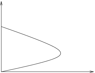
For , the only solution satisfying all the above requirements is for and . Then we have a double root structure, which means that the corresponding brane world solution is of compact sections. It is important to note that in this case the horizon positions are bounded from above and , so the corresponding Hubble parameters are going to be bounded from below. When in particular , the two roots become degenerate and . The solution deserves special attention and will be discussed later on. The plot of the horizon (or brane) positions as a function of is given in Fig.1. It is important to stress that the relevant black hole solution corresponding to this soliton, has the characteristics, of a de-Sitter-Schwarzschild like black hole studied in [31]. Note that the bigger the the smaller the effective cosmological constant. Here we have a pure Gauss-Bonnet soliton (or black hole) in the sense that the limit is singular.
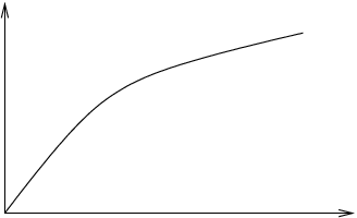
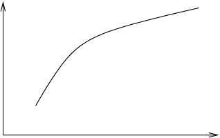
For , i.e. in the Einstein branch, we have two classes of solutions. The first class is for and . The single horizon of that case can take all positive values. The second class is for and . In this case the horizon position is bounded from below as . Furthermore, in the latter case the singularity (12) exists and is hidden behind the horizon. In the limit , we have and the brane position becomes singular. We should therefore exclude the point from the physical parameter space. In both cases, the brane Hubble parameter can be as small as desired. The plots of the horizon position as a function of in the above cases is given in Fig.2. It is interesting to note that both cases here correspond to a Gauss-Bonnet corrected six dimensional Schwarzschild black hole solution with or .
4.1.2 The vacua
Vacua with , which are , exist only in the Gauss-Bonnet branch. In the Einstein branch, for all the cases satisfying the constraint (15), the region shielded by the horizon is timelike and therefore not suitable for our compactification.
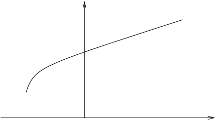
In the Gauss-Bonnet branch , we have only non-compact brane world models, all of them for . The solutions satisfy the criteria (14)-(16) for . The singularity (12) exists for but is always hidden behind the horizon. The plots of the horizon position as a function of in the above cases is given in Fig.3.
4.1.3 The Nariai vacuum
The degenerate case for in the Gauss-Bonnet branch deserves special consideration. This happens when the mass parameter reaches its maximal value and so the two horizons become one, . The internal space then appears to collapse, however one should look as for the Nariai metric to a different coordinate system [39]. So, setting , we make the coordinate transformation that consists of an affine transformation
| (27) | |||||
| (28) |
The degenerate case corresponds to the limit and as can be seen from (18), it is the limit that the four-dimensional part of the metric is rendered unwarped. In these coordinates and with
| (29) |
The affine transformation blows up a point of the coordinate system to a well behaved internal space in the coordinates. Let us now define the modified potential
| (30) |
with the parameters and as functions of and given by
| (31) |
Then, substituting everything in the metric (18) we obtain the blown up metric
| (32) |
The Nariai limit gives a non-singular limit for the modified potential . Therefore, we obtain a non-vanishing internal space
| (33) |
Note that, after this coordinate transformation, the deficit angle from (21) can be expressed as a function of the modified potential as
| (34) |
Thus, in this limit the deficit angle is independent of and depends only on the periodicity of the angular coordinate.
4.1.4 Zero black hole mass
Let us now suppose that also the black hole mass vanishes . Then, the potential has the simple cosmological form
| (35) |
from where we can see that the Einstein branch can only give the trivial flat six-dimensional solution, for . The Gauss-Bonnet branch on the other hand has non-trivial solutions. The flat case is excluded since it has no horizon, but there are and solutions. Firstly, the case can have brane world solutions as long as . Then the spacelike region that we use for the internal space is non-compact. This case corresponds to the point of Fig.3 where the curve intersects the axis.
On the other hand, for the vacua we can have an horizon for and obtain a compact brane world model which is part of a six dimensional de-Sitter space. This case corresponds to the point of Fig.1 where the upper curve of intersects the axis. Furthermore, since the space has no singularity at , we can extend the radial coordinate to and consider the region of . The internal space is symmetric around , thus we have symmetry around the equator of the internal space. The reintroduction of a black hole mass breaks this symmetry since it introduces an singularity.
4.1.5 Flat vacuum
As noted before, the black hole ansatz (18) does not admit flat vacua for . However, this ansatz, as we noticed also in the Nariai vacuum, has limitations, since it describes only warped four-dimensional metrics. Looking for unwarped solutions, it is easy to see that the following flat vacuum is a trivial solution of the equations of motion (3)
| (36) |
where . It is non-compact and exists for any sign of . The equations (23), (24), (25) continue to hold for . To compactify such flat vacua, a gauge field flux has to be added along the lines of Appendix A.
4.2 Non-zero bulk cosmological constant
Let us now switch on the bulk cosmological constant, i.e. . The polynomial (16) is more complicated to solve, therefore we will study some special cases and focus on as few parameters as possible. Namely, the case with zero black hole mass and also the point in parameter space where the theory can be written in a BI form. Finally, we will provide all the flat () vacua.
4.2.1 Zero black hole mass
If the black hole mass vanishes , the potential has the simple cosmological form
| (37) |
It is obvious that the only brane world solutions that we can obtain in the present case are the curved ones .
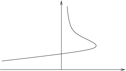
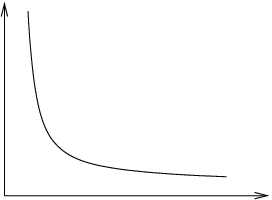
Let us first discuss the () solutions. For , we see from (15) that only the Einstein branch has a solution with a horizon. Furthermore, in this case, in order to have , the bulk cosmological constant should be positive, i.e. . For we can have solutions both in the Einstein and the Gauss-Bonnet branch. In the Einstein branch the horizon is for positive bulk cosmological constant with . On the other hand, in the Gauss-Bonnet branch there are solutions for any . At the BI limit the two branches merge to a unique solution. In all the above cases the spacelike region is for and the internal spaces are compact. As in Sec.4.1.4, we can extend the radial coordinate to and consider the region of , since the space has no singularity at . The plots of the horizon position as a function of in the above cases are given in Fig.4.
The () solutions are the same as above if we substitute . Thus, the curves in Fig.4 should be the mirrors of the case with respect to the axis. In addition, the spacelike region for these solutions is for , thus all the vacua are for non-compact internal spaces.
4.2.2 The Born-Infeld vacua
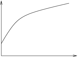
For the and vacua, it is easy to see that is monotonic for and has an extremum at if .
The vacua obtained for deserve special attention. As discussed in the Sec.2, these vacua do not have an Einstein limit. In a certain way they correspond to the strongly coupled limit of the Gauss-Bonnet term in the action (1), since at the linearized level the combination multiplies the perturbation operator. Furthermore, as we saw in the previous section, for these vacua the branches for , merge. Let us now switch on a mass parameter in the potential and write it as
| (38) |
where the integration constant replaces . The potential (38) is similar to an Einstein black hole potential in four dimensions with a cosmological constant, apart from the fact that the Newtonian potential is now rather than ! Furthermore, if we were to compare it with the six dimensional Einstein black hole (), we see that gravity in the Born-Infeld case is far weaker as one approaches the singularity.
Keeping this comparison in mind, the flat vacua of this theory, exist for and are non-compact. In order for the region to be spacelike, we need and thus (similar to a planar black hole). The horizon position is simply . We will see more of the flat vacua in the last subsection.
For the case , the potential has only one root. In order for the region to be spacelike, we need to have . Then both cases are possible. For the () vacua, the horizon distance is bounded from below , while for the () vacua, the horizon is not bounded. The plot of the horizon positions as a function of is given in Fig.5. The situation is similar to an Schwarzschild black hole with planar or spherical horizon.
In the , the potential has either none or two roots. In order for the potential to acquire two roots the black hole mass should be in the range . Then we can distinguish two possible cases, one with and , and a second with and . For the () vacua, the spacelike region is for and thus the space is non-compact. The horizon is bounded as . For the () vacua, the spacelike region is for and thus the space is compact. The outer horizon is bounded as and the inner as . When the two roots become degenerate and . This solution will be discussed in the following section. The plot of the horizon positions as a function of is given in Fig.6.
4.2.3 The Born-Infeld Nariai vacuum
The degenerate case of the Born-Infeld vacuum for , and deserves special consideration. This happens when and so . The internal space then appears to collapse, however one should look as for the Nariai metric in a different coordinate system, as we saw in Sec.4.1.3. Repeating the same procedure as before and expressing the parameters and as functions of and
| (39) |
we find that the Nariai limit gives a non-singular limit for the modified potential . Therefore, we obtain a non-vanishing internal space
| (40) |
Furthermore, the deficit angle from (21) can be expressed as a function of the modified potential as
| (41) |
4.2.4 Flat vacua
Let us now study the flat () vacua that exist in the case. We have found previously a flat vacuum in the special BI case. More generally, we know from (15) that flat vacua can exist only for . The horizon position is at and we can see from the potential asymptotics that the region will be spacelike in two cases: (i) and and (ii) and . Thus, for both cases we should have . In case (i) there is a branch cut singularity given in (12) hidden always beyond the horizon. In case (ii) there is not such .
In all these cases, the flat vacua have non-compact internal spaces and are warped. The latter property is in contrast to the flat vacuum that exists when . Thus, we see that the introduction of a bulk cosmological constant can be compensated by the black hole mass and warping of the four-dimensional space, giving again vacua of zero four-dimensional curvature. As noted before, to compactify such flat vacua, a gauge field flux has to be added along the lines of Appendix A.
5 Self-properties of the solutions
Let us now discuss the physical consequences of the above solutions. In particular, we wish to see whether we can obtain codimension-2 braneworlds exhibiting self-accelerating or self-tuning behaviour. For the former, we seek models where the acceleration is mainly of geometrical origin rather than due to the vacuum energy or tension of the branes. For the latter, we seek braneworld solutions (de Sitter or flat) where the effective Hubble parameter of the brane is not related to the brane vacuum energy and the tension can be arbitrary large even for small observable Hubble curvature. Here it is important to emphasize, that the Gauss-Bonnet term plays the role of an induced gravity term on the brane [23] according to (22). Therefore even if the internal space is not compact we expect that gravity will be four dimensional up to some distance scale. In fact, we would expect, and this turns out to be true, that self-acceleration will hold for warped but uncompactified codimension-2 setups as for the case of codimension-1. Secondly, taking into account that the effective curvature of the brane is given by
| (42) |
i.e. as the sum of a geometrical term and a brane tension term, the self-accelerating and the self-tuning cases are, in some respect, in contrast to each other.
Let us first study self-acceleration. The key relation is (42). For this case, one should firstly have a non-zero positive geometrical contribution to the curvature, i.e. coming from the Gauss-Bonnet term in the action (1). Secondly, this contribution should be dominant in comparison to the brane tension contribution. Note that in order to be in accord with phenomenology from supernovae data [1] and since , the Gauss-Bonnet coupling should be roughly of the order . In this case, the Gauss-Bonnet term in the action is dominant in comparison to the Einstein-Hilbert term. Furthermore, for this limit, even the compact models will have enormous volumes of cosmological size, and therefore will be comparable to certain aspects of infinite volume ones (see Appendix C for the calculation of the volumes of the various models).
It is useful to define a self-acceleration index as the fraction of the geometrical acceleration to the curvature
| (43) |
When we have assuming . On the other hand, if , we have with the limit giving . We can argue that self-acceleration exists whenever , with the strict self-accelerating limit being for .
The index (43) depends on the specific bulk solutions that we have. Going through the vacua that we discussed in the previous section, we should restrict ourselves to the ones with . Then the self-acceleration index for the various cases is listed as following
- 1.
For , , , we have two horizons and the index for the two branes varies as and . Thus, for this case (Fig.1) we have no strict self-accelerating limit. The Nariai limit case gives .
- 2.
For , , , we have one horizon and the index is (Fig.2). Here we have a strict self-accelerating limit when , however, at the model is singular.
- 3.
For , , , , we have the compact -symmetric model with .
- 4.
For , , , , we have the compact -symmetric model (Fig.4). The index for is and for varies as . The strict self-accelerating limit happens for the BI case and can be approached by either branch and . One can argue that the BI limit is natural in the sense that the theory becomes more symmetric at that point.
- 5.
For the BI case with , , , we have two horizons (Fig.6) and the index for the two branes varies as and . The strict self-accelerating limit happens for the case as mentioned above.
From the above we see that the two physically interesting cases where the late acceleration of our Universe can be of purely geometrical origin, are cases 2 and 4. In case 2 the strict limit can only be reached asymptotically in order not to hit the singularity at .
Actually, the first two cases present some similarities and one important difference with the codimension-1 DGP [8], which is worth noting. In fact, we see that case 2 corresponds to the self-accelerating branch of DGP [14] and case 1 to that of the normal branch with branes [11]. A first similarity is the fact that we obtain branching, which now is in-between the Gauss-Bonnet branch and the Einstein branch. Secondly, for case 1, as for the normal branch with branes, we expect a normalisable spin-2 graviton since the relevant volume element is finite. It is an intriguing difference, however, that the codimension-1 unstable or self-accelerating branch corresponds to the Einstein branch here and not the Gauss-Bonnet one.
In case 4, we note that the limit is regular and we see that around , self-acceleration is possible for both branches. Here, the similarity with codimension-1 resides that in that the case of tension we have enhanced symmetry [10, 11], as one also expects for the Born-Infeld case in codimension-2.
Let us now discuss the cases which have to do with self-tuning. The self-tuning idea aims to allow for vacua where their effective cosmological constant is independent from (or at least not strongly dependent on) the vacuum energy of the brane, without fine-tuning. In the toy-model we are presenting here, vacuum energy is represented by the brane tension whereas the effective cosmological constant is represented by . For self-tuning to operate, there should be enough integration constants allowed to be adjusted when we vary one brane tension, with the crucial demand of keeping the curvature of that brane constant. In the solutions that we have discussed, the free parameters are the angular coordinate range and the black hole mass . On the other hand, the action parameters are the Gauss-Bonnet coupling , the bulk cosmological constant and the brane tensions . If we vary for instance we do not wish , , , to change, but only possibly and . We will be obviously interested in the and the flat vacua to test if such a self-tuning can work.
For the vacua, the Hubble parameter on the brane depends on the black hole mass and the action parameters and . Since we require that the action parameters are not tuned, if we fix the curvature this is equivalent to fixing the black hole mass . In the cases where we have more than one brane with different Hubble parameters , both of the latter are given functions of , and . Thus, fixing from the curvature of the one brane , fixes also the curvature of the second brane . Then from the relation
| (44) |
we see that, if we change , we can keep the curvature constant by changing . But since is fixed, we have to change also . This results to an interbrane fine-tuning. Hence, the only way to obtain self-tuning is when the second brane is absent, or in -symmetric models where only one of the above relations survive.
These selftuning cases, however, are not all theoretically satisfying if we look at the orders of magnitude of the various dimensionful quantities in (42). Although we have no idea of the brane tension value today, it would be logical that, if no accurate cancellations happen during phase transitions in the history of the Universe, its natural order of magnitude is . On the other hand we know that the the present value of the Hubble constant is approximately . In order that (42) can then be satisfied, today’s curvature should be negligible in comparison with . In other words, we should find models which allow for and approximately
| (45) |
The above relation should not be viewed as a fine tuning between the action parameters and , since scales as (23) and can vary in time when the vacuum energy changes, in accordance with the remarks of [35]. The constraints on the time variation of Newton’s constant come rather late in the history of the Universe, certainly after the QCD phase transition. Therefore, the relation (45) is providing the angle deficit/excess parameter , given a Gauss-Bonnet coupling , which needs not to be unnatural as in the self-accelerating case. Furthermore, the relation (45) is exact for the case of flat vacua.
From the models that we have discussed, let us see the cases that give rise to such theoretically viable self-tuning
- •
For , , and for both and , we have the non-compact vacua with for (see Fig.2).
- •
For , , , , we have -symmetric vacua with for (see Fig.4).
- •
For , , , , we have non-compact vacua with for (see Fig.4).
- •
For the BI case with , , we have non-compact with for (see Fig.5).
- •
All the flat non-compact vacua, for both and are self-tuning in the exact sense.
Here we should note once more that the above (exact or approximate) self-tuning solutions do not constitute a resolution, but rather a potential amelioration, of the cosmological constant problem. We have found vacua where the brane curvature is independent of the brane vacuum energy and furthermore the these two energy scales can be well separated. However, the important question, for which the self-tuning mechanism cannot give a simple answer, is if the dynamical variation of the vacuum energy results in remaining in these vacua. In some sense, the term self-tuning itself is deceiving since the existence of these vacua does not guarantee that there are some attractor dynamics which tune the system towards them. Nevertheless, the very existence of them is important, since at least at the level of non-dynamical solutions, dissociating the brane curvature from its vacuum energy is a rather unique situation. Moreover, we saw that most of these vacua are non-compact, but, as we will explain in the last section, gravity is quasi-localised and thus effectively four dimensional up to some cross-over scale.
It is evident that the vacua with the above self-tuning properties are different from the ones with the self-accelerating properties corresponding in particular to a totally different bare parameter . This is true as long as we want self-acceleration at a very low energy scale. If, for example, we want to explain inflation theory geometrically, as in [36], then the self-accelerating (inflationary) vacua can be deformed to self-tuning ones by letting the integration constant run. A nice toy model scenario for this is pictured in Fig.2 if we assume that is an increasing function of proper cosmological time. One starts at the big-bang singularity which corresponds to a 6 dimensional bulk naked singularity at . At early time we have and the inflationary expansion is, . At late time the late expansion is related to the large mass of the soliton whereas the vacuum energy is of the order of which is much larger than the current Universe curvature .
Before we close off this section, it is worth pointing out that no self-tuning cases are possible for the Gauss-Bonnet branch. Furthermore, the only finite volume self-tuning case that we encountered is possible for a de Sitter braneworld.
6 The Gauss-Bonnet instantons
In our previous analysis, we have found several brane world vacua of finite volume. These solutions are of special interest because they can give rise to gravitational instantons. We saw how they all have the feature that the four dimensional space is . Wick rotating to a Euclidean metric as in (5) with and keeping the Euclidean internal space, all the coordinates are spacelike and the solutions describe a Riemannian manifold with conical singularities. Particularly important are the instantons which are regular, in other worlds those having no conical singularities (see also [37, 38]). We can divide these vacua into two classes according to their topology.
The first class of instantons are the ones for vanishing black hole mass , where there is no singularity at and the space is -symmetric. These instantons are given by
| (46) |
with and are topologically . In order for these instantons to be regular, one should have , which from (21) gives for the periodicity of the -coordinate. These instantons have an Einstein theory limit only in the case and .
The second class of instantons are the ones of the Nariai limits of vacua with non-vanishing black hole mass found in Sec.4.1.3 and Sec.4.2.3. These instantons are given by
| (47) |
where is a numerical factor and the degenerate horizon. These instantons, in contrast with the ones noted before, are topologically . In order for these to be regular, one should have . The deficit angle for the instantons that we have found is given by , thus, regularity of the instantons imposes . Let us also note here that these instantons for the case , exist also for the case other that the BI limit that we have discussed in Sec.4.2.3. This is why in (47) we allowed for dependence of the degenerate horizon. None of these instantons has an Einstein theory limit.
The above instantons have the physical interpretation of describing probabilities of nucleation processes [39, 40] between two distinct gravitational backgrounds. In particular, the probability of nucleation of a pair of Nariai black holes from the pure backgrounds of , is given by
| (48) |
where is the one loop contribution from the quantum quadratic fields and and are the values of the action for the two instantons that we presented earlier. It is straightforward to compute the above probability of nucleation for the two simple cases of and the BI case . In both cases one obtains
| (49) |
Since these action differences are positive definite, we deduce that the probability of both processes is unsuppressed unlike the case of [39]. Therefore, the solitonic vacua () are apparently stable with respect to pure de Sitter vacua in Lovelock theory. This result certainly deserves further study.
7 Discussion and Conclusions
In this paper we studied in some detail codimension-2 braneworlds in the context of Lovelock gravity. Using a modified version of Birkhoff’s staticity theorem [24, 25], we found all six dimensional solutions describing a de Sitter, flat or anti de Sitter braneworld of codimension 2. First thing we can observe is that, unlike the codimension-1 case where the Gauss-Bonnet invariant plays a somewhat secondary role, here, in the case of codimension-2 braneworlds, it can give rise to self-acceleration and certain self-tuning properties which are not present in the Einstein theory. This is largely due to the fact that codimension-2 junction conditions induce on the brane an Einstein-Hilbert term [22]. It is important to note that this does not mean that we have ordinary four-dimensional gravity, rather, as noted in [23], we are in a quite similar situation as for the codimension-1 DGP model [8]. By this, we mean that from some ultraviolet scale up to some infrared scale we expect gravity to ”look” four-dimensional. A proof of this statement of course requires the full spectrum of gravitational perturbations for the solutions that we have found.
The important relation we came across is (25) which relates the vacuum energy or tension of the brane with the Gauss-Bonnet coupling and the effective cosmological expansion on the brane , which itself is related to the characteristics of the bulk solution: its mass, bulk cosmological constant (and charge) in particular. The interesting feature we found here is that the Gauss-Bonnet coupling can give de Sitter branes without vacuum energy on the brane, purely geometrically. In this sense such de Sitter solutions are self-accelerating. In order to explain the small cosmological constant we then have to fine-tune as usual .
The second important point is that Gauss-Bonnet coupling and the topological parameter , which is otherwise unconstrained, dictate the cross-over scale between the four-dimensional Planck scale and the six-dimensional one (23). Here, unlike the five dimensional DGP model, the cross over scale is not necessarily tied up to the self-acceleration scale. Indeed, the more is close to 1 (23), the more we can dissociate these scales. In a nutshell, all depends on the gravity phenomenology beyond the cross-over scale and is dictated by the full graviton propagator on the brane. As we emphasized, the appearance of the induced Einstein tensor in the codimension-2 junction conditions is not a proof of an effective four-dimensional gravity or not. It is a definite sign, however, that a relevant scale will appear in the boundary conditions for the gravitational perturbations. Although we have not undertook the precise perturbation calculation here, we will comment on some of its characteristics later on.
The most conservative approach is, as in DGP [14], to introduce a hierarchy of scales between and so that the cross-over scale is
| (50) |
Assuming that , this gives a very low higher dimensional Planck scale which in turn dictates that . But, as mentioned above, one can have by having . For the self-tuning vacua, on the other hand, the natural value of the Gauss-Bonnet coupling is which for the same cross-over scale (50) and gives a huge angle excess . Obviously, in this case a reasonable hierarchy between and the cross-over scale , cannot reduce significantly the latter huge excess angle. We emphasize, however, that the above orders of magnitude, should be viewed with caution since the definition of the cross-over scale (50) should be done in a true cosmological setting with complete knowledge of the modified FRW equations.
Another important point concerns the fact that the self-accelerating branch of DGP seems to be embedded in the usual Einstein branch of Lovelock theory and not in the Gauss-Bonnet branch. Indeed, given the Gauss-Bonnet term in the action and no bare cosmological constant () we find two distinct solutions for (7): in the Gauss-Bonnet branch, , we can have a finite volume soliton solution since then the Gauss-Bonnet coupling plays the role of a cosmological constant (Fig.1) (situation akin to a Schwarzschild de Sitter black hole [31]). Then, we have a finite volume element and we expect a normalisable zero mode graviton. We get no self-acceleration. For the Einstein branch however, , we have a single brane, infinite volume element and self acceleration with as small tension as we want (Fig.2). The bulk solution corresponds to a Gauss-Bonnet corrected Schwarzschild black hole. This difference may be interesting in respect to linear (in)stability and the presence of ghosts of such backgrounds, not only in the scalar, but also in the spin-2 sector.
Furthermore, in our solutions we see at least two different length scales emerging where we can probe differing four-dimensional gravity. That of the volume element, which if finite, would mean that beyond that scale we expect ordinary four-dimensional gravity. Secondly, that of the cross-over scale where up to that distance gravity seems four-dimensional, as in the case of the codimension-1 DGP model. Again we emphasize that the cross over scale and self acceleration scale are here supplemented by an extra topological parameter which in a sense tells us how far we are from a Kaluza-Klein setup for the Killing direction . Indeed, we see that for our codimension-2 space is very much like a lightning rod [41], where we seemingly have a cascade from a six-dimensional to a five-dimensional and then a four-dimensional setup (reminiscent of the recent proposal [42]).
What is missing from our analysis is the linear perturbation of these solutions which will tell us of the stability and the precise gravitational spectrum. This is not a trivial task, for our metric is not conformally flat. Therefore, apart from the usual complications of black hole perturbations, one has to add the fact that Lovelock perturbations are going to be genuinely different from the usual ones for Einstein theory. The reason is simple: the background Weyl tensor appears in the Lovelock field equations and thus, extra tensor pieces are bound to appear for tensorial perturbations. Recent work in fact from string theory [43], in relation to the /CFT correspondence, indicates that there is yet another scale appearing in the bulk perturbations of (6). This extra scale comes from the extra tensorial pieces ”to be added” to the usual perturbation operator, that dictate that gravity waves in a planar () black hole background (6) can evolve in a differing background geometry than that of (6). This means in particular that the light-cone of the wave fronts can break causality. We think that this is an intriguing and extremely important issue, which we hope will be undertaken soon.
In addition, the cosmology of codimension-2 branes is very poorly understood, especially from the point of view of self-tuning and the issue of vacuum selection. It has been known that in Einstein gravity the introduction of matter other than tension on codimension-2 branes introduces singularities33 3 This is a well known fact in four dimensional gravity, called the Israel paradox concerning self-gravitating cosmic string metrics (see for example [44]). worse than conical [45] (see, however, the work of [46] for intersecting brane cosmology in six dimensions). Although, the appearance of singularities is natural in defects of codimension higher than one [47, 48], one has in practice to regularise the brane [49, 50] in order to consider some cosmological fluid on them [51, 52]. Although one expects that brane singularities persist in the Lovelock theory, the fact that there exists an induced Einstein equation on the brane, allows for the cosmology to be studied without the need of explicit regularisation. We plan to address the question of cosmology of the present Lovelock models in a different publication [53].
Acknowledgments
It is a great pleasure to acknowledge discussions and numerous insightful comments from Nemanja D. Kaloper, Kozuya Koyama and Antonio H. Padilla. We thank them also for reading through the manuscript. We also thank Roy Maartens for bringing up the issue of self acceleration in the context of codimension-2 braneworlds early on. C.C. also thanks Emilian Dudas and Valery Rubakov for discussions and critical comments. A.P. is supported by a Marie Curie Intra-European Fellowship EIF-039189.
Appendix A: A more general action
In this Appendix we will consider a generalization of the model that we discussed in the main text to a -dimensional bulk spacetime, where also a gauge field is coupled to gravity. The action of the system reads
| (A.1) |
where the -dimensional Newton’s constant.
It is straightforward to write down the Einstein equations of motion for the above action. They read
| (A.2) |
with the energy momentum tensor
| (A.3) |
Furthermore, the gauge field equation reads
| (A.4) |
The static spherically symmetric solutions of the above equations of motion with -dimensional space of maximal symmetry are locally isometric to
| (A.5) |
The explicit solution of the equations of motion then gives
| (A.6) |
and for the potential,
| (A.7) |
and the parameters appearing in the action have been rescaled to,
| (A.8) |
The integration constants are,
| (A.9) |
where is the charge, is the AD or ADM mass of the solution and is the area of the unit maximally symmetric subspace. Finally, which gives rise to 2 branches of solutions. The convention of the sign is chosen so that the gravitational mass is always . As one can easily check by expanding the square root for large distances, the sign flip in front of is necessary to match the Schwarzschild solution behaviour for positive AD mass. On the other hand, the charge term of the above potential is the opposite of a charged black hole for .
Appendix B: The general solution of
To determine the positions of the horizons for the case, we need the general solutions of the third order algebraic equation
| (B.1) |
The solutions of the above equation depend on the parameters , and in particular on the discriminant of the system
| (B.2) |
If there is only one real root. If there are three real roots, two of which become degenerate where the inequality saturates. A critical value of that will be useful in the subsequent study is
| (B.3) |
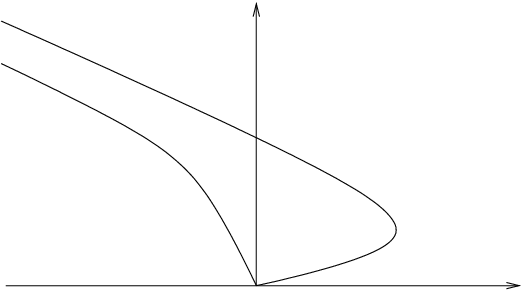
Since the solutions of the above equation will correspond to horizons, we also need to look which of these real roots are in addition positive. All permissible cases are listed as following
- •
If and , it is and we have the root
(B.4) - •
If and , it is , but we have one positive root which is given by the same formula as above (B.4). [It has different value, however, since .]
- •
If and , it is and we have two roots
(B.5) (B.6) - •
If and , it is but we only have one positive root, given by (B.5).
The results of the above analysis are summarized in Fig.7.
Appendix C: Volume calculation
In this Appendix, we will calculate the volume of the general brane world models that we considered in the main text. To do this, we will make the assumption that the zero mode graviton wavefunction follows the warp factor. In other words, we will assume that the zero mode is emanating from the metric
| (C.1) |
with the four dimensional metric , where is a perturbation around the background . To find the volume of the space we should substitute the metric (C.1) in the action (1) and integrate out the internal space. We will define the volume (Vol) to be given by the coefficient of the four-dimensional curvature term in the action as44 4 Notice that according to the ansatz (C.1), it is and thus . For this reason, we obtain an unusual mass dimension for the volume . With a suitable four-dimensional coordinate rescaling, e.g. , the volume will be redefined as and will acquire the correct mass dimension.
| (C.2) |
where the dots represent higher order in curvature terms. It is straightforward to compute that the various quantities of the action (1) for the ansatz (C.1) give
| (C.3) | |||||
| (C.4) | |||||
| (C.5) |
Then the volume is given by the following integral
| (C.6) |
If , the above integral gives
| (C.7) |
where F is the hypergeometric function
| (C.8) |
For the special BI case, , the integral gives instead
| (C.9) |
It is straightforward to see that the above formulas give finite (and positive) volume for the two Nariai cases. To obtain the volume in this case one should move to the coordinates and take the limit .
References
- [1] A. G. Riess et al. [Supernova Search Team Collaboration], Astron. J. 116 (1998) 1009 [arXiv:astro-ph/9805201]; S. Perlmutter et al. [Supernova Cosmology Project Collaboration], Astrophys. J. 517 (1999) 565 [arXiv:astro-ph/9812133]; A. G. Riess et al. [Supernova Search Team Collaboration], Astrophys. J. 607 (2004) 665 [arXiv:astro-ph/0402512].
- [2] S. M. Carroll, Living Rev. Rel. 4 (2001) 1 [arXiv:astro-ph/0004075]; J. Polchinski, arXiv:hep-th/0603249; R. Bousso, Gen. Rel. Grav. 40 (2008) 607 [arXiv:0708.4231 [hep-th]].
- [3] S. Weinberg, Rev. Mod. Phys. 61 (1989) 1.
- [4] S. M. Carroll, Phys. Rev. Lett. 81 (1998) 3067 [arXiv:astro-ph/9806099]; C. F. Kolda and D. H. Lyth, Phys. Lett. B 458 (1999) 197 [arXiv:hep-ph/9811375]; N. Kaloper and L. Sorbo, JCAP 0604 (2006) 007 [arXiv:astro-ph/0511543].
- [5] C. M. Will, Living Rev. Rel. 9 (2005) 3 [arXiv:gr-qc/0510072]; C. M. Will, Theory and experiment in gravitational physics, Cambridge University Press.
- [6] L. Amendola, D. Polarski and S. Tsujikawa, Int. J. Mod. Phys. D 16 (2007) 1555 [arXiv:astro-ph/0605384].
- [7] I. I. Kogan, S. Mouslopoulos, A. Papazoglou, G. G. Ross and J. Santiago, Nucl. Phys. B 584 (2000) 313 [arXiv:hep-ph/9912552]; R. Gregory, V. A. Rubakov and S. M. Sibiryakov, Phys. Rev. Lett. 84 (2000) 5928 [arXiv:hep-th/0002072].
- [8] G. R. Dvali, G. Gabadadze and M. Porrati, Phys. Lett. B 485 (2000) 208 [arXiv:hep-th/0005016].
- [9] I. I. Kogan, S. Mouslopoulos, A. Papazoglou and L. Pilo, Nucl. Phys. B 625 (2002) 179 [arXiv:hep-th/0105255]; R. Gregory, V. A. Rubakov and S. M. Sibiryakov, Phys. Lett. B 489 (2000) 203 [arXiv:hep-th/0003045].
- [10] D. Gorbunov, K. Koyama and S. Sibiryakov, Phys. Rev. D 73 (2006) 044016 [arXiv:hep-th/0512097]; K. Koyama, Phys. Rev. D 72 (2005) 123511 [arXiv:hep-th/0503191].
- [11] C. Charmousis, R. Gregory, N. Kaloper and A. Padilla, JHEP 0610 (2006) 066 [arXiv:hep-th/0604086].
- [12] G. Dvali, New J. Phys. 8 (2006) 326 [arXiv:hep-th/0610013].
- [13] C. Charmousis, R. Gregory and A. Padilla, JCAP 0710 (2007) 006 [arXiv:0706.0857 [hep-th]].
- [14] C. Deffayet, Phys. Lett. B 502 (2001) 199 [arXiv:hep-th/0010186].
- [15] N. Kaloper, Phys. Rev. Lett. 94 (2005) 181601 [Erratum-ibid. 95 (2005) 059901] [arXiv:hep-th/0501028]; N. Kaloper, Phys. Rev. D 71 (2005) 086003 [Erratum-ibid. D 71 (2005) 129905] [arXiv:hep-th/0502035]; K. Koyama and F. P. Silva, Phys. Rev. D 75 (2007) 084040 [arXiv:hep-th/0702169].
- [16] C. de Rham and A. J. Tolley, JCAP 0607 (2006) 004 [arXiv:hep-th/0605122].
- [17] N. Arkani-Hamed, S. Dimopoulos, N. Kaloper and R. Sundrum, Phys. Lett. B 480 (2000) 193 [arXiv:hep-th/0001197]; S. Kachru, M. B. Schulz and E. Silverstein, Phys. Rev. D 62 (2000) 045021 [arXiv:hep-th/0001206]; S. Forste, Z. Lalak, S. Lavignac and H. P. Nilles, Phys. Lett. B 481 (2000) 360 [arXiv:hep-th/0002164]; S. Forste, Z. Lalak, S. Lavignac and H. P. Nilles, JHEP 0009 (2000) 034 [arXiv:hep-th/0006139]; C. Csaki, J. Erlich and C. Grojean, Nucl. Phys. B 604 (2001) 312 [arXiv:hep-th/0012143]; J. E. Kim, B. Kyae and H. M. Lee, Nucl. Phys. B 613 (2001) 306 [arXiv:hep-th/0101027]; P. Binetruy, C. Charmousis, S. C. Davis and J. F. Dufaux, Phys. Lett. B 544 (2002) 183 [arXiv:hep-th/0206089]; C. Charmousis, S. C. Davis and J. F. Dufaux, JHEP 0312 (2003) 029 [arXiv:hep-th/0309083].
- [18] J. W. Chen, M. A. Luty and E. Ponton, JHEP 0009 (2000) 012 [arXiv:hep-th/0003067].
- [19] S. M. Carroll and M. M. Guica, arXiv:hep-th/0302067; I. Navarro, JCAP 0309 (2003) 004 [arXiv:hep-th/0302129]; Y. Aghababaie, C. P. Burgess, S. L. Parameswaran and F. Quevedo, Nucl. Phys. B 680 (2004) 389 [arXiv:hep-th/0304256]; I. Navarro, Class. Quant. Grav. 20 (2003) 3603 [arXiv:hep-th/0305014]; G. W. Gibbons, R. Guven and C. N. Pope, Phys. Lett. B 595 (2004) 498 [arXiv:hep-th/0307238]; J. M. Schwindt and C. Wetterich, Phys. Lett. B 578 (2004) 409 [arXiv:hep-th/0309065]; C. P. Burgess, F. Quevedo, G. Tasinato and I. Zavala, JHEP 0411 (2004) 069 [arXiv:hep-th/0408109].
- [20] A. Kehagias, Phys. Lett. B 600 (2004) 133 [arXiv:hep-th/0406025]; S. Randjbar-Daemi and V. A. Rubakov, JHEP 0410 (2004) 054 [arXiv:hep-th/0407176]; H. M. Lee and A. Papazoglou, Nucl. Phys. B 705 (2005) 152 [arXiv:hep-th/0407208]; A. Kehagias and C. Mattheopoulou, Nucl. Phys. B 797 (2008) 117 [arXiv:0710.4021 [hep-th]].
- [21] D. Lovelock, J. Math. Phys. 12 (1971) 498; B. Zumino, Phys. Rept. 137 (1986) 109 .
- [22] P. Bostock, R. Gregory, I. Navarro and J. Santiago, Phys. Rev. Lett. 92 (2004) 221601 [arXiv:hep-th/0311074].
- [23] C. Charmousis and R. Zegers, JHEP 0508 (2005) 075 [arXiv:hep-th/0502170]; C. Charmousis and R. Zegers, Phys. Rev. D 72 (2005) 064005 [arXiv:hep-th/0502171].
- [24] D. L. Wiltshire, Phys. Lett. B 169 (1986) 36; C. Charmousis and J. F. Dufaux, Class. Quant. Grav. 19 (2002) 4671 [arXiv:hep-th/0202107].
- [25] R. Zegers, J. Math. Phys. 46 (2005) 072502 [arXiv:gr-qc/0505016].
- [26] D. G. Boulware and S. Deser, Phys. Rev. Lett. 55 (1985) 2656.
- [27] R. G. Cai, Phys. Rev. D 65 (2002) 084014 [arXiv:hep-th/0109133].
- [28] J. Crisostomo, R. Troncoso and J. Zanelli, Phys. Rev. D 62 (2000) 084013 [arXiv:hep-th/0003271].
- [29] S. Deser and B. Tekin, Phys. Rev. D 67 (2003) 084009 [arXiv:hep-th/0212292]; A. Padilla, Class. Quant. Grav. 20 (2003) 3129 [arXiv:gr-qc/0303082].
- [30] R. Gregory and A. Padilla, Phys. Rev. D 65 (2002) 084013 [arXiv:hep-th/0104262].
- [31] R. C. Myers and J. Z. Simon, Phys. Rev. D 38 (1988) 2434.
- [32] Z. C. Wu, Phys. Lett. B 612 (2005) 115 [arXiv:hep-th/0405249].
- [33] S. Mukohyama, Y. Sendouda, H. Yoshiguchi and S. Kinoshita, JCAP 0507 (2005) 013 [arXiv:hep-th/0506050].
- [34] B. Linet, J. Math. Phys. 27 (1986) 1817.
- [35] H. P. Nilles, A. Papazoglou and G. Tasinato, Nucl. Phys. B 677 (2004) 405 [arXiv:hep-th/0309042].
- [36] A. A. Starobinsky, Phys. Lett. B 91 (1980) 99.
- [37] R. Gregory, N. Kaloper, R. C. Myers and A. Padilla, JHEP 0710 (2007) 069 [arXiv:0707.2666 [hep-th]].
- [38] C. Garraffo, G. Giribet, E. Gravanis and S. Willison, arXiv:0711.2992 [gr-qc].
- [39] P. H. Ginsparg and M. J. Perry, Nucl. Phys. B 222 (1983) 245.
- [40] S. W. Hawking, G. T. Horowitz and S. F. Ross, Phys. Rev. D 51 (1995) 4302 [arXiv:gr-qc/9409013]; O. J. C. Dias and J. P. S. Lemos, Phys. Rev. D 70 (2004) 124023 [arXiv:hep-th/0410279].
- [41] N. Kaloper and D. Kiley, JHEP 0705 (2007) 045 [arXiv:hep-th/0703190].
- [42] C. de Rham, G. Dvali, S. Hofmann, J. Khoury, O. Pujolas, M. Redi and A. J. Tolley, arXiv:0711.2072 [hep-th]; C. de Rham, S. Hofmann, J. Khoury and A. J. Tolley, JCAP 0802 (2008) 011 [arXiv:0712.2821 [hep-th]].
- [43] M. Brigante, H. Liu, R. C. Myers, S. Shenker and S. Yaida, arXiv:0802.3318 [hep-th]; M. Brigante, H. Liu, R. C. Myers, S. Shenker and S. Yaida, arXiv:0712.0805 [hep-th].
- [44] J. A. G. Vickers, Class. Quant. Grav. 4 (1987) 1; V. P. Frolov, W. Israel and W. G. Unruh, Phys. Rev. D 39 (1989) 1084; W. G. Unruh, G. Hayward, W. Israel and D. Mcmanus, Phys. Rev. Lett. 62 (1989) 2897; B. Boisseau, C. Charmousis and B. Linet, Phys. Rev. D 55 (1997) 616 [arXiv:gr-qc/9607029].
- [45] J. M. Cline, J. Descheneau, M. Giovannini and J. Vinet, JHEP 0306 (2003) 048 [arXiv:hep-th/0304147].
- [46] H. M. Lee and G. Tasinato, JCAP 0404 (2004) 009 [arXiv:hep-th/0401221]; O. Corradini, K. Koyama and G. Tasinato, arXiv:0712.0385 [hep-th]; O. Corradini, K. Koyama and G. Tasinato, arXiv:0803.1850 [hep-th].
- [47] C. Charmousis, R. Emparan and R. Gregory, JHEP 0105 (2001) 026 [arXiv:hep-th/0101198].
- [48] N. Kaloper and D. Kiley, JHEP 0603 (2006) 077 [arXiv:hep-th/0601110].
- [49] M. Kolanovic, M. Porrati and J. W. Rombouts, Phys. Rev. D 68 (2003) 064018 [arXiv:hep-th/0304148]; S. Kanno and J. Soda, JCAP 0407 (2004) 002 [arXiv:hep-th/0404207]; I. Navarro and J. Santiago, JHEP 0502 (2005) 007 [arXiv:hep-th/0411250].
- [50] M. Peloso, L. Sorbo and G. Tasinato, Phys. Rev. D 73 (2006) 104025 [arXiv:hep-th/0603026]; E. Papantonopoulos, A. Papazoglou and V. Zamarias, JHEP 0703 (2007) 002 [arXiv:hep-th/0611311]; C. P. Burgess, D. Hoover and G. Tasinato, JHEP 0709 (2007) 124 [arXiv:0705.3212 [hep-th]].
- [51] E. Papantonopoulos, A. Papazoglou and V. Zamarias, Nucl. Phys. B 797 (2008) 520 [arXiv:0707.1396 [hep-th]]; M. Minamitsuji and D. Langlois, Phys. Rev. D 76 (2007) 084031 [arXiv:0707.1426 [hep-th]].
- [52] J. Vinet and J. M. Cline, Phys. Rev. D 70 (2004) 083514 [arXiv:hep-th/0406141]; J. Vinet and J. M. Cline, Phys. Rev. D 71 (2005) 064011 [arXiv:hep-th/0501098]; F. Chen, J. M. Cline and S. Kanno, Phys. Rev. D 77 (2008) 063531 [arXiv:0801.0226 [hep-th]].
- [53] C. Charmousis, G. Kofinas, A. Papazoglou, work in progress.