跳到论文正文
W Papers独立论文阅读器 arXiv:0804.2044 论文正文 计算阅读时间 · 0%
引用这篇论文根据当前论文元数据生成,正式投稿前建议核对。


License: arXiv.org perpetual non-exclusive license
arXiv:0804.2044v1 [hep-ph] 13 Apr 2008

QED in finite volume and finite size scaling effect on electromagnetic properties of hadrons

Preprint: 
Shunpei Uno Affiliation: Department of Physics, Nagoya University, Nagoya, Aichi 464-8602, Japan Email: uno@eken.phys.nagoya-u.ac.jp Affiliation: Email:
Abstract: 

On account of its application to the present and future analysis of the virtual photon correction to the hadronic properties by means of lattice QCD simulation, we initiate the study of the finite size scaling effect on the QED correction using low energy effective theory of QCD with QED. For this purpose, we begin with formulating a new QED on the space with finite volume. By adapting this formalism to the partially quenched QCD with electromagnetism, we explore the qualitative features of the finite size scaling effect on the electromagnetic correction to the masses of pseudo-Goldstone bosons.

Keywords: 
Chiral Lagrangians, Electromagnetic Processes and Properties, NLO Computations, Lattice QCD

1 Introduction

The recent progress in the lattice QCD simulation enables us to perform “measurements” for hadronic properties through the world with more and more realistic QCD realized in the computer. It may not be a far future that the lattice QCD simulation becomes a method by which precise measurement of nonperturbative dynamics of QCD is reached.

One of the important applications of the lattice QCD simulation would be the determination of quark masses. The light quark masses have been determined using dynamical quarks with two flavors [1, 2, 3, 4, 5, 6] and (2+1)(2+1) flavors [7, 8, 9, 10]. The forthcoming precise measurement through the lattice QCD simulation reminds us that quarks are electrically charged. All of the hadronic properties thus suffer from electromagnetic (EM) radiative corrections. Because the EM interaction is other source of explicit breaking of isospin symmetry than the difference between the masses mu,mdm_{u},\,m_{d} of up and down-quarks, the determination of mu−mdm_{u}-m_{d} requires us to grasp the size of EM correction quantitatively at the hadronic level. Among the references [1, 2, 3, 4, 5, 6, 7, 8, 9, 10], Ref. [8] is the only work that presented the values of mum_{u}, mdm_{d} each, but it does not seem to make the data fit with a function parametrizing the EM splitting in the kaon masses as an undetermined constant.

The attempt to incorporate EM correction to the pseudoscalar meson masses in the context of lattice simulation was first done by Duncan et al.[11] by simulating QED put on the lattice. By adopting the same technique to incorporate QED correction, the QED correction to the meson masses has been investigated with use of dynamical domain wall fermions with two-flavors [12], and in the quenched approximation with the renormalization group improved gauge action [13]. Ref. [14] employs another method to calculate the leading-order EM correction to Δ​mπ2≡mπ+2−mπ02\Delta m_{\pi}^{2}\equiv m_{\pi^{+}}^{2}-m_{\pi^{0}}^{2} in the two-flavor overlap fermion simulation. This work relies on the formula [15]

Δ​mπ2|α\displaystyle\left.\Delta m_{\pi}^{2}\right|_{\alpha} =\displaystyle= 3​α4​π​fπ2​∫d4​ki⁡(2​π)​Dμ​ν​(k)\displaystyle\frac{3\,\alpha}{4\pi f_{\pi}^{2}}\int\frac{d^{4}k}{i\left(2\pi\right)}D^{\mu\nu}(k)\, (1)
×∫d4​x​ei​k⋅x​[⟨Vμ3​(x)​Vν3​(0)⟩QCD−⟨Aμ3​(x)​Aν3​(0)⟩QCD],\displaystyle\quad\times\int d^{4}x\,e^{ik\cdot x}\left[\left<V^{3}_{\mu}(x)\,V^{3}_{\nu}(0)\right>_{\rm QCD}-\left<A^{3}_{\mu}(x)\,A^{3}_{\nu}(0)\right>_{\rm QCD}\right]\,,

where Dμ​ν​(k)=ημ​ν/(k2+i​ϵ)D^{\mu\nu}(k)=\eta^{\mu\nu}/(k^{2}+i\epsilon) is the photon propagator, fπf_{\pi} (≃92\simeq 92 MeV) is the pion decay constant, Vμa≡q¯​Ta​γμ​qV^{a}_{\mu}\equiv\overline{q}T^{a}\gamma_{\mu}q and Aμa≡q¯​Ta​γν​γ5​qA^{a}_{\mu}\equiv\overline{q}T^{a}\gamma_{\nu}\gamma_{5}q with the normalization of S​U​(2)SU(2) generators tr⁡(Ta​Tb)=12​δa​b{\rm tr}\,\left(T^{a}T^{b}\right)=\frac{1}{2}\,\delta^{ab}. ⟨𝔒⟩QCD\left<\mathfrak{O}\right>_{\rm QCD} denotes the expectation value of the operator 𝔒\mathfrak{O} with respect to QCD. The lattice simulation calculates the two correlation functions appearing on the right-hand side of Eq. (1) and attempts to get the pion mass difference in the chiral limit [14].

Though our interest is the nonperturbative dynamics of QCD on space with infinite volume, the simulation has to be done in the virtual world with finite volume. As quarks with colors and electric charges must live in such a finite volume, it is inevitable that QED correction suffers from finite size scaling effect no matter what computational method one may choose. It is plausible that two pseudoscalar mesons in a common isospin multiplet share the same QCD finite size corrections [16, 17, 18, 19, 20, 21, 22, 23, 24, 25, 26, 27, 28]. In addition, electromagnetic force is long-ranged. Therefore the finite size scaling effect regarding QED will dominate the finite size corrections in the EM splittings. Unless it is adequately quantified, ignorance on the QED finite size scaling effect becomes another source of systematic uncertainty in mu−mdm_{u}-m_{d} derived using lattice simulation.

Thus far, there are diametrical opposite views on the relevance of QED finite size scaling. The authors in Ref. [13] performed the direct (quenched) lattice QCD measurement of the EM splitting in pion masses using two different sizes of four-volumes, T×L3=24​a×(12​a)3T\times L^{3}=24a\times(12a)^{3} and 24​a×(16​a)324a\times(16a)^{3}, where aa is the lattice spacing. They observed no significant difference for the EM splitting measured in two volumes and concluded that a linear size L=2.4L=2.4 fm is sufficient to compute the EM splitting without correcting the measured values within available statistical uncertainty. Contrastingly, Refs. [11, 12] estimated the QED finite size scaling according to the one-pole saturation approximation [15, 29, 30] to Eq. (1) with the momentum integral replaced with the sum

Δ​mπ2|α,VMD​(T,L)\displaystyle\left.\Delta m_{\pi}^{2}\right|_{\alpha,\,{\rm VMD}}(T,\,L) =\displaystyle= 3​α4​π​(4​π)2​1T​1L3​∑k∈(Γ~4−{0})mV2​mA2k2​(k2+mV2)​(k2+mA2),\displaystyle\frac{3\alpha}{4\pi}\left(4\pi\right)^{2}\frac{1}{T}\frac{1}{L^{3}}\sum_{k\in\left(\widetilde{\Gamma}_{4}-\left\{0\right\}\right)}\frac{m_{V}^{2}m_{A}^{2}}{k^{2}\left(k^{2}+m_{V}^{2}\right)\left(k^{2}+m_{A}^{2}\right)}\,, (2)

where mV≃770m_{V}\simeq 770 MeV, mA≃970m_{A}\simeq 970 MeV is the mass of A1A_{1} in the chiral limit, and

Γ~4\displaystyle\widetilde{\Gamma}_{4} ≡\displaystyle\equiv {k=(k0,k1,k2,k3)|k0∈2​πTℤ,kj∈2​πLℤ},\displaystyle\left\{k=(k_{0},\,k_{1},\,k_{2},\,k_{3})\left|k_{0}\in\frac{2\pi}{T}\,\mathbb{Z}\,,k_{j}\in\frac{2\pi}{L}\,\mathbb{Z}\right.\right\}\,, (3)

is a lattice on the Euclidean four-momentum space. For the lattice geometry T×L3=32​a×(16​a)3T\times L^{3}=32a\times(16a)^{3} with 1/a≃1.661/a\simeq 1.66 GeV in Ref. [12], Eq. (2) leads

Δ​mπ2|α,VMD​(T,L)Δ​mπ2|α,VMD​(∞,∞)≃0.9,\displaystyle\frac{\left.\Delta m_{\pi}^{2}\right|_{\alpha,\,{\rm VMD}}(T,\,L)}{\left.\Delta m_{\pi}^{2}\right|_{\alpha,\,{\rm VMD}}(\infty,\,\infty)}\simeq 0.9\,, (4)

which is not negligible.

Under such circumstances, we investigate the finite size scaling effect on the QED contribution to light pseudoscalar meson masses using the chiral perturbation theory including electromagnetism [31, 32, 33, 34, 35]. Though the finial quantitative determination of the finite size correction must resort to the first principle calculation as in Ref. [13], any qualitative understanding as shown here will help one to make extrapolation to infinite volume in the future simulation study.

This paper actually consists of two parts. In the first part, Sec. 2, we give a formulation of QED on the space with finite volume. This task is necessary because a single classical charged particle does not satisfy the equation of motion, say, the Gauss’ law constraint in the finite volume QED obtained via the ordinal compactification procedure. This is intuitively understandable as the electric flux emanating from a nonzero charge finds nowhere else to go. We thus begin with defining such a QED that accommodates a single charged particle on the space ℝ×𝕋3\mathbb{R}\times\mathbb{T}^{3}, where 𝕋3\mathbb{T}^{3} is three-dimensional torus corresponding to the compact space. The second part, Sec. 3, utilizes this QED to study the finite size scaling effect on the electromagnetic splittings in pseudoscalar meson masses. For this purpose, the calculation is performed in the framework of the partially quenched chiral perturbation theory [36, 37, 38, 39] including the electromagnetism [33] in view of its practical application to the actual lattice simulation . Sec. 4 is denoted to discussion and conclusion. Appendix A collects the formulae for the basic sums which appear in the evaluation of finite size scaling effect.

2 QED in finite volume

The aim of this section is to present a new QED on the space with finite volume, which allows us to investigate the properties of a single charged particle. We first clarify in Sec. 2.1 the problem itself that confronts us in the QED obtained by the ordinal compactification procedure. In Sec. 2.2, we define a new QED in finite volume and explain how it solves this problem. Throughout this paper, the topology of the space is the three-dimensional torus 𝕋3≡𝕊1×𝕊1×𝕊1\mathbb{T}^{3}\equiv\mathbb{S}^{1}\times\mathbb{S}^{1}\times\mathbb{S}^{1} with a common circumference LL for all 𝒮1\mathcal{S}^{1}. A point on 𝕋3\mathbb{T}^{3} is thus specified by the coordinates 𝐱≡(x1,x2,x3){\bf x}\equiv(x^{1},\,x^{2},\,x^{3}) obeying periodicity xj≅xj+Lx^{j}\cong x^{j}+L (j=1, 2, 3j=1,\,2,\,3). As in the analysis of finite size scaling of QCD [16, 17, 18], the temporal direction t=x0t=x^{0} is taken to be infinite, t∈ℝt\in\mathbb{R}, for single particle states to develop poles in the energy space. We adopt the convention ημ​ν=diag⁡(1,−1,−1−1)\eta_{\mu\nu}={\rm diag\left(1,\,-1,\,-1\,-1\right)} for the signature of the metric.

2.1 problem

The most familiar procedure to construct the corresponding theory on 𝕋3\mathbb{T}^{3} is to impose periodic boundary conditions on all fields. The electromagnetic theory obtained via such a naïve ℤ3\mathbb{Z}^{3}-orbifolding procedure 11 1 The word naïve means here that the Fourier modes A~μ​(t,𝐤=𝟎)\widetilde{A}_{\mu}(t,\,{\bf k}={\bf 0}) in Eq. (12) are treated as basic variables. We recall that the Wilson lines is appropriate variables. The correct 𝒵3\mathcal{Z}^{3}-orbifolding would involve the integration over Wilson line U0​(t)∼exp⁡[i​e​∫d​t​1L3​A~0​(t, 0)]U_{0}(t)\sim\exp\left[i\,e\int dt\,\frac{1}{L^{3}}\,\widetilde{A}_{0}(t,\,{\bf 0})\right] which leads to the constraint that the charges on every three-dimensional hypersurface should vanish in total 1L3​∫d3​𝐱​j0​(t,𝐱)=0.\displaystyle\frac{1}{L^{3}}\int d^{3}{\bf x}\,j^{0}(t,\,{\bf x})=0\,. (5) We would like to see what happens in the naïve procedure. is referred to as QEDℤ3{}_{\mathbb{Z}^{3}} here. In QEDℤ3{}_{\mathbb{Z}^{3}} the gauge potential Aμ​(x)A_{\mu}(x) (xν=(t,𝐱)x^{\nu}=(t,\,{\bf x})), in particular, obeys periodic boundary condition in every spatial direction. This form of boundary condition is motivated for the practical reason that the periodic or anti-periodic boundary condition is imposed along spatial directions for the available lattice QCD configurations and the conservation of quantized momenta at every QED vertex requires that every spatial component of photon momenta be an integer multiple of 2​πL\frac{2\pi}{L}. The action for the gauge kinetic term in QEDℤ3{}_{\mathbb{Z}^{3}} takes the usual form

Sγ\displaystyle S_{\gamma} =\displaystyle= ∫d​t​∫𝕋3d3​𝐱​(−14​Fμ​ν​Fμ​ν),\displaystyle\int dt\int_{\mathbb{T}^{3}}d^{3}{\bf x}\,\left(-\frac{1}{4}\,F_{\mu\nu}\,F^{\mu\nu}\right)\,, (6)

with the field strength Fμ​ν=∂μAν−∂νAμF_{\mu\nu}=\partial_{\mu}A_{\nu}-\partial_{\nu}A_{\mu}.

To elucidate the problem from the practical point of view in our context, we go back to Eq. (2) for the EM splitting in the pion mass squared in the effective theory including the vector and axial-vector mesons. The application of the ℤ3\mathbb{Z}^{3}-orbifolding procedure to the effective Lagrangian including the vector and axial-vector mesons in Ref. [30] immediately leads the same form of the Lagrangian written in terms of the spatially periodic fields. This effective theory gives the expression for the EM splitting in Eq. (2) with T→∞T\rightarrow\infty

Δ​mπ2|α,VMD​(∞,L)\displaystyle\left.\Delta m_{\pi}^{2}\right|_{\alpha,\,{\rm VMD}}(\infty,\,L) =\displaystyle= 3​α4​π​(4​π)2​∫−∞∞d​k02​π​1L3​∑𝐤∈Γ~3mV2​mA2k2​(k2+mV2)​(k2+mA2),\displaystyle\frac{3\alpha}{4\pi}\left(4\pi\right)^{2}\int_{-\infty}^{\infty}\frac{dk^{0}}{2\pi}\frac{1}{L^{3}}\sum_{{\bf k}\in\widetilde{\Gamma}_{3}}\frac{m_{V}^{2}m_{A}^{2}}{k^{2}\left(k^{2}+m_{V}^{2}\right)\left(k^{2}+m_{A}^{2}\right)}\,, (7)

where

Γ~3\displaystyle\widetilde{\Gamma}_{3} ≡\displaystyle\equiv {𝐤=(k1,k2,k3)|kj∈2​πLℤ}.\displaystyle\left\{{\bf k}=\left(k^{1},\,k^{2},\,k^{3}\right)\left|\,k^{j}\in\frac{2\pi}{L}\,\mathbb{Z}\right.\right\}\,. (8)

We can see that the quantity (7) has infrared (IR) divergence coming from the contribution of 𝐤=𝟎{\bf k}={\bf 0}. The expression (7) can be interpreted as the sum of the contribution of Kaluza-Klein modes in one-dimensional field theory. The IR divergence appearing in Eq. (8) is attributed to that of a massless mode from this point of view. It should be reminded that Δ​mπ2|α,VMD\left.\Delta m_{\pi}^{2}\right|_{\alpha,\,{\rm VMD}} in infinite volume is IR-finite. Therefore, limL→∞Δ​mπ2|α,VMD​(∞,L)≠Δ​mπ2|α,VMD\displaystyle{\lim_{L\rightarrow\infty}\left.\Delta m_{\pi}^{2}\right|_{\alpha,\,{\rm VMD}}(\infty,\,L)\neq\left.\Delta m_{\pi}^{2}\right|_{\alpha,\,{\rm VMD}}}. The theory deducing Eq. (7) is one of QEDℤ3{}_{\mathbb{Z}^{3}} with the content of matter fields and the action concretely specified. The same pathology always emerges in every QEDℤ3{}_{\mathbb{Z}^{3}} theory irrespective of the details of the matter fields and the action. Thus QEDℤ3{}_{\mathbb{Z}^{3}} cannot be used to study the finite size scaling effect on the EM splittings.

The origin of the above pathology will be traced back to the inconsistency of a single charged particle with the classical equation of motion. Though it may be well-known, the detail observation of this point will help us to grasp the essence of our new QED. Due to the periodicity of the gauge potential, the electromagnetic current jμ​(x)≡δ​Smatter/δ​Aμ​(x)j^{\mu}(x)\equiv\delta S_{\rm matter}/\delta A_{\mu}(x) derived from the matter part SmatterS_{\rm matter} of the action is also periodic along the spatial directions. The current jμ​(x)j^{\mu}(x) is assumed to be conserved under the equations of motion derived from the variation of matter fields. The classical equation of motion derived from the variation of Aμ​(x)A_{\mu}(x) is hence

∂νFμ​ν​(x)=jμ​(x).\displaystyle\partial_{\nu}F^{\mu\nu}(x)=j^{\mu}(x)\,. (9)

This contains the Gauss’ law constraint

∇⋅𝐄⁡(x)=ρ⁡(x).\displaystyle{\bf\nabla}\cdot{\bf E}(x)=\rho(x)\,. (10)

where the electric field Ej​(x)E^{j}(x) and the charge density ρ⁡(x)\rho(x) are given by Ej​(x)=F0​j​(x)E^{j}(x)=F^{0j}(x) and ρ​(x)=j0​(x)\rho(x)=j^{0}(x), respectively. For simplicity, we consider an infinitely heavy charged particle. When it is at rest initially, the charge density and the profile of electric field are both constant in time

∇⋅𝐄⁡(𝐱)=e​δ3​(𝐱).\displaystyle{\bf\nabla}\cdot{\bf E}({\bf x})=e\,\delta^{3}({\bf x})\,. (11)

The inconsistency appears when both sides of this equation are integrated over the whole 𝕋3\mathbb{T}^{3}; the left-hand side vanishes while the right-hand side does not. Likewise, we can see that any single charged particle cannot live on 𝕋3\mathbb{T}^{3}.

2.2 new QED on ℝ×𝕋3\mathbb{R}\times\mathbb{T}^{3}

The observation in Sec. 2.1 shows that the IR divergence in Eq. (7) is a manifestation of inconsistency of a single charged particle with the classical equation of motion. The aim of this section is to introduce an alternative QED in finite volume that solves this problem for the sake of our study of the finite size scaling effect on the EM splitting.

In the space 𝕋3\mathbb{T}^{3}, three-momenta take discrete values in Γ~3\widetilde{\Gamma}_{3} in Eq. (8). Accordingly, the gauge potential is decomposed in the Fourier series with respect to the spatial dimension

Aμ​(t,𝐱)\displaystyle A_{\mu}(t,\,{\bf x}) =\displaystyle= 1L3​∑𝐤∈Γ~3ei​𝐤⋅𝐱​A~μ​(t,𝐤).\displaystyle\frac{1}{L^{3}}\sum_{{\bf k}\in\widetilde{\Gamma}_{3}}e^{i{\bf k}\cdot{\bf x}}\,\widetilde{A}_{\mu}(t,\,{\bf k})\,. (12)

The new QED on ℝ×𝕋3\mathbb{R}\times\mathbb{T}^{3}, referred to as QEDL, is the theory without variables A~μ​(t,𝐤=𝟎)\widetilde{A}_{\mu}(t,\,{\bf k}={\bf 0}) ab initio. In other words, we do not incorporate the Wilson lines Uμ​(t)∼exp⁡[i​e​∫d​t​1L3​A~μ​(t, 0)]U_{\mu}(t)\sim\exp\left[i\,e\,\int dt\,\frac{1}{L^{3}}\widetilde{A}_{\mu}(t,\,{\bf 0})\right] as dynamical variables. In terms of such a gauge potential, the action of pure electromagnetism is given by SγS_{\gamma} in Eq. (6). Below, we observe the various features possessed by QEDL.

First, we see how QEDL solves the problems in Sec. 2.1. The equation of motion is modified as follows. Since the modes A~μ​(t, 0)\widetilde{A}_{\mu}(t,\,{\bf 0}) are absent, the variation of the full action S=Sγ+SmatterS=S_{\gamma}+S_{\rm matter} with respect to the gauge potential becomes

δA​S\displaystyle\delta_{A}S =\displaystyle= ∫−∞∞d​t​∫𝕋3d3​𝐱​[−12​δ​Fμ​ν​Fμ​ν+δ​Aμ​jμ]\displaystyle\int_{-\infty}^{\infty}dt\int_{\mathbb{T}^{3}}d^{3}{\bf x}\left[-\frac{1}{2}\delta F_{\mu\nu}F^{\mu\nu}+\delta A_{\mu}\,j^{\mu}\right] (13)
=\displaystyle= ∫−∞∞dt∑𝐤∈Γ~3′[δAμ(t,𝐤)\displaystyle\int_{-\infty}^{\infty}dt\sum_{{\bf k}\in\widetilde{\Gamma}_{3}^{\prime}}\left[\delta A_{\mu}(t,\,{\bf k})\right.
×∫d3𝐱ei​𝐤⋅𝐱(−∂νFμ​ν(t,𝐱)+jμ(t,𝐱))],\displaystyle\qquad\qquad\qquad\left.\times\int d^{3}{\bf x}\,e^{i{\bf k}\cdot{\bf x}}\left(-\partial_{\nu}F^{\mu\nu}(t,\,{\bf x})+j^{\mu}(t,\,{\bf x})\right)\right]\,,

where

Γ~3′≡Γ~3−{𝟎}.\displaystyle\displaystyle{\widetilde{\Gamma}_{3}^{\prime}\equiv\widetilde{\Gamma}_{3}-\left\{{\bf 0}\right\}\,.} (14)

As the result, the extremum condition gives the equations of motion only for 𝐤≠𝟎{\bf k}\neq{\bf 0};

∫d3​𝐱​cos⁡(𝐤⋅𝐱)​{∂νFμ​ν​(t,𝐱)−jμ​(t,𝐱)}=0(𝐤≠𝟎).\displaystyle\displaystyle{\int d^{3}{\bf x}\,\cos\left({\bf k}\cdot{\bf x}\right)\left\{\partial_{\nu}F^{\mu\nu}(t,\,{\bf x})-j^{\mu}(t,\,{\bf x})\right\}=0\quad({\bf k}\neq{\bf 0})\,.} (15)

The inconsistency seen in Sec. 2.1 is therefore circumvented. We also note that Eq. (15) instead of Eq. (10) no longer yields the equality between the charges contained in a domain VV in 𝕋3\mathbb{T}^{3} and the electric flux penetrating the surface ∂V\partial V.

The quantum field theory will be defined in the path integral framework by defining the measure of the gauge potential as usual. Let δ​A~μ​(t,𝐤)\delta\widetilde{A}_{\mu}(t,\,{\bf k}) be an infinitesimal variation of the mode A~μ​(t,𝐤)\widetilde{A}_{\mu}(t,\,{\bf k}) (t∈ℝt\in\mathbb{R},  𝐤∈Γ~3′{\bf k}\in\widetilde{\Gamma}_{3}^{\prime}). The functional measure is defined corresponding to the norm in the space of gauge configurations in QEDL

‖δ​A‖2≡∫d​t​∑𝐤∈Γ~3′δ​A~μ​(t,𝐤)​δ​A~μ​(t,𝐤).\displaystyle\left\|\delta A\right\|^{2}\equiv\int dt\sum_{{\bf k}\in\widetilde{\Gamma}_{3}^{\prime}}\delta\widetilde{A}_{\mu}(t,\,{\bf k})\,\delta\widetilde{A}^{\mu}(t,\,{\bf k})\,. (16)

As we will see later this norm will turn out to be gauge-invariant. From the point of view of field theory on ℝ\mathbb{R}, A~​(t, 0)\widetilde{A}(t,\,{\bf 0}) are massless fields. Due to the absence of these modes in QEDL, the IR divergence as in Eq. (8) no longer appears.

We next observe the gauge symmetry of QEDL. The transformation of the gauge potential is given by

Aμ​(x)↦Aμ′​(x)=Aμ​(x)+∂μΛ,\displaystyle A_{\mu}(x)\mapsto A^{\prime}_{\mu}(x)=A_{\mu}(x)+\partial_{\mu}\Lambda\,, (17)

while a matter field Φ⁡(x)\Phi(x) with charge QΦ​eQ_{\Phi}e is transformed as

Φ​(x)↦Φ′​(x)\displaystyle\Phi(x)\mapsto\Phi^{\prime}(x) =\displaystyle= exp⁡[i​QΦ​e​Λ​(x)]​Φ​(x).\displaystyle\exp[iQ_{\Phi}\,e\,\Lambda(x)]\,\Phi(x)\,. (18)

Here we assume that there is at least one matter field which has the minimum charge ee. The easiest way to identify the full gauge symmetry is to look at the full gauge symmetry of QEDℤ3{}_{\mathbb{Z}^{3}} first. There, the general form of Λ⁡(x)\Lambda(x) that keeps the periodic boundary condition for the matter fields takes the form

Λ⁡(x)\displaystyle\Lambda(x) =\displaystyle= ΛP​(x)+2​πe​L​∑j=13mj​xj(QEDℤ3),\displaystyle\Lambda_{P}(x)+\frac{2\pi}{e\,L}\,\sum_{j=1}^{3}m_{j}x^{j}\quad\left({\rm QED}_{\mathbb{Z}^{3}}\right)\,, (19)

where mj∈ℤm_{j}\in\mathbb{Z}, and ΛP​(x)\Lambda_{P}(x) is periodic along 𝕋3\mathbb{T}^{3}.

Denoting the Fourier components of ΛP​(t,𝐱)\Lambda_{P}(t,\,{\bf x}) by Λ~P​(t,𝐤)\widetilde{\Lambda}_{P}(t,\,{\bf k}), the gauge transformation for the gauge potential becomes in the three-momentum space

A~j′​(t,𝐤)\displaystyle\widetilde{A}^{\prime}_{j}(t,\,{\bf k}) =\displaystyle= A~j​(t,𝐤)+(i​kj​Λ^P​(t,𝐤)+L3​δ𝐤, 0​2​πe​L​mj)(QEDℤ3).\displaystyle\widetilde{A}_{j}(t,\,{\bf k})+\left(ik^{j}\widehat{\Lambda}_{P}(t,\,{\bf k})+L^{3}\,\delta_{{\bf k},\,{\bf 0}}\,\frac{2\pi}{e\,L}\,m_{j}\right)\quad({\rm QED}_{\mathbb{Z}^{3}})\,. (20)

In our new QED, A~​(t, 0)\widetilde{A}(t,\,{\bf 0}) no longer exists. It thus turns out that there are no redundancy corresponding to 𝐦∈ℤ3{\bf m}\in\mathbb{Z}^{3} and time-dependent but spatially homogeneous part of ΛP​(x)\Lambda_{P}(x), that is,

A~j′​(t,𝐤)\displaystyle\widetilde{A}^{\prime}_{j}(t,\,{\bf k}) =\displaystyle= A~j​(t,𝐤)+i​kj​Λ^P​(t,𝐤)(QEDL),\displaystyle\widetilde{A}_{j}(t,\,{\bf k})+i\,k^{j}\widehat{\Lambda}_{P}(t,\,{\bf k})\quad\left({\rm QED}_{L}\right)\,, (21)

where

∂tΛ~P​(t, 0)=0.\displaystyle\displaystyle{\partial_{t}\widetilde{\Lambda}_{P}(t,\,{\bf 0})=0\,.} (22)

One can readily see that the set of all functions that fulfill Eq. (22) forms an abelian group. From Eq. (21), it is also easy to see that this gauge group is exactly the redundancy that allows us to take the Coulomb gauge fixing condition

∂jAj​(t,𝐱)=0.\displaystyle\partial_{j}A_{j}(t,\,{\bf x})=0\,. (23)

We recall that in QEDℤ3{}_{\mathbb{Z}^{3}} a residual gauge symmetry survives even after imposing the condition (23), which should be fixed by the additional condition A~0​(t, 0)=0\widetilde{A}_{0}(t,\,{\bf 0})=0 [12]. In contrast, the condition (23) suffices to fix redundancy in QEDL leaving only the global symmetry. Obviously, the norm (16) in the space of gauge configurations is gauge-invariant. We can also make a BRST complex by introducing the ghost fields corresponding to the gauge parameters of the form (22) in the standard manner [40].

We close this section with a few remarks. We consider the scattering of a charged particle and its anti-particle in the center of mass frame, leaving aside the issue whether the scattering may not be well-defined in the presence of a long-ranged force in finite volume. Due to the absence of the modes A~μ​(t, 0)\widetilde{A}_{\mu}(t,\,{\bf 0}), the ss-channel process mediated by a single virtual photon does not occur. However, we recall that Lorentz invariance, in particular, the symmetry related to the Lorentz boosts, is explicitly violated on the space ℝ×𝕋3\mathbb{R}\times\mathbb{T}^{3}. Thus, once we consider the collision say, of an incident charged particle with three-momentum (p+2​πL)​𝐞x(p+\frac{2\pi}{L}){\bf e}_{x}, where p∈2​πL​ℤp\in\frac{2\pi}{L}\mathbb{Z} and 𝐞x{\bf e}_{x} is a unit three-vector along xx-direction, and an anti-particle with momentum (−p)​𝐞x(-p){\bf e}_{x}, the ss-channel process occurs. In the limit L→∞L\rightarrow\infty, the cross section will approach to that in the center of mass frame in infinite volume.

Secondly, since the equation of motion (15) is not written locally, QEDL seems to possess somewhat non-locality. In fact, it is not still clear at the present stage whether this is actually the case, and then whether another pathology appears in QEDL. As will be demonstrated explicitly in the subsequent section, even if non-locality is present, it is so mild that the structure of ultra-violet (UV) divergence in QEDL remains completely the same as in QED in infinite volume. This feature is contrasted the situation in noncommutative field theory [41, 42, 43]; the the UV structure of a noncommutative field theory differs significantly from that of the commutative counterpart due to the hard non-locality.

3 Finite size scaling in meson mass

Now we apply QEDL to the study of finite size effect on the EM correction to the pseudoscalar meson masses in the chiral perturbation theory including the electromagnetism [31, 32, 33, 34]. Looking at the practical application to the lattice simulation, we adopt the partially quenched chiral perturbation theory [36, 37, 38, 39] including the electromagnetism [33] and compute the leading-order finite size correction to the EM splitting in this theory. For that purpose, we begin with summarizing our notations for partially quenched chiral perturbation theory including electromagnetism to the next-leading order. We derive the formulas for the next-to-leading order correction to the pseudoscalar meson mass in finite volume, and evaluate them numerically to investigate the finite size correction to the EM splitting.

3.1 partially quenched chiral perturbation theory with electromagnetism

The next-to-leading order corrections to the off-diagonal meson masses has already been computed in Ref. [33]. However, the expression written by the momentum integrals are needed in practice for the study of finite size scaling effect. To derive such an expression in Sec. 3.2, we fix the notations, in particular, of the low-energy constants at the next-to-leading order for the subsequent calculation, and dictate the free meson propagators necessary for the one-loop calculation. To take the application to the partially quenched system with two-flavors, the super-trace of the EM charge matrix 𝒬~\widetilde{\mathcal{Q}} is not assumed here to vanish, unlike in Ref. [33]. There then appear more local terms at the next-to-leading order (i,e., O⁡(p4)O(p^{4}), O⁡(e2​p2)O(e^{2}p^{2}) and O⁡(e4)O(e^{4})) than those found in Ref. [33]. We list up all of them by drawing upon Appendix of Ref. [32] where one-loop UV divergences were computed for generic flavor number NFN_{F} in the unquenched chiral perturbation theory including electromagnetism. After that, we compute the UV divergences that should be absorbed by the coefficients of these local terms.

In what follows, all the fields and parameters are written in the “flavor” basis

𝔔\displaystyle\mathfrak{Q} ≡\displaystyle\equiv (q1V,⋯,qNVV,q1S,⋯,qNSS,g1,⋯,gNV)T,\displaystyle\left(q^{V}_{1},\,\cdots,\,q^{V}_{N_{V}},\,q^{S}_{1},\,\cdots,\,q^{S}_{N_{S}},\,g_{1},\,\cdots,\,g_{N_{V}}\right)^{T}\,, (24)

where qrSq^{S}_{r} (r=1,⋯,NSr=1,\,\cdots,\,N_{S}) denote the sea quark fields, qαVq^{V}_{\alpha} (α=1,⋯,NV\alpha=1,\,\cdots,\,N_{V}) the valence quark fields, and gαg_{\alpha} (α=1,⋯,NV\alpha=1,\,\cdots,\,N_{V}) the ghost quark fields [36]. The chiral symmetry is a graded Lie group G=S​U​(NS+NV|NV)L×S​U​(NS+NV|NV)RG=SU(N_{S}+N_{V}|N_{V})_{L}\times SU(N_{S}+N_{V}|N_{V})_{R}. It breaks down spontaneously to its vector-like subgroup H=S​U​(NS+NV|NV)VH=SU(N_{S}+N_{V}|N_{V})_{V}. The associated Nambu-Goldstone bosons are represented by an (NS+NV|NV)×(NS+NV|NV)(N_{S}+N_{V}|N_{V})\times(N_{S}+N_{V}|N_{V}) supermatrix Π\Pi. Using

u⁡[Π⁡(x)]\displaystyle u[\Pi(x)] =\displaystyle= exp⁡(i​Π⁡(x)2​F0),\displaystyle\exp\left(i\,\frac{\Pi(x)}{\sqrt{2}\,F_{0}}\right)\,, (25)

Π\Pi transforms nonlinearly under (gL,gR)∈G(g_{L},\,g_{R})\in G through

u⁡[Π]↦u⁡[Π′]=gR​u​[Π]​h​((gL,gR),Π)†=h⁡((gL,gR),Π)​u​[Π]​gL†.\displaystyle u[\Pi]\mapsto u[\Pi^{\prime}]=g_{R}\,u[\Pi]\,h((g_{L},\,g_{R});\,\Pi)^{\dagger}=h((g_{L},\,g_{R});\,\Pi)\,u[\Pi]\,g_{L}^{\dagger}\,. (26)

where h⁡((gL,gR),Π)∈Hh((g_{L},\,g_{R});\,\Pi)\in H. We follow the convention for the chiral Lagrangian which can be read off from Refs. [33, 44] with minor modification.

The external fields Rμ​(x)R_{\mu}(x), Lμ​(x)L_{\mu}(x) that couple to the right-handed and left-handed chiral components of vector currents are incorporated in the partially quenched QCD action for the purpose of calculating the connected Green functions of vector and axial-vector currents. They are defined to transform under local (gL,gR)(g_{L},\,g_{R}) as

Lμ↦Lμ′=gL​Lμ​gL†+i​gL​∂μgL†,\displaystyle\displaystyle{L_{\mu}\mapsto L^{\prime}_{\mu}=g_{L}L_{\mu}\,g_{L}^{\dagger}+ig_{L}\,\partial_{\mu}g_{L}^{\dagger}\,,}
Rμ↦Rμ′=gR​Rμ​gR†+i​gR​∂μgR†.\displaystyle\displaystyle{R_{\mu}\mapsto R^{\prime}_{\mu}=g_{R}R_{\mu}\,g_{R}^{\dagger}+ig_{R}\,\partial_{\mu}g_{R}^{\dagger}\,.} (27)

The field strengths

Lμ​ν=∂μLν−∂νLμ−[Lμ,Lν],Rμ​ν=∂μRν−∂νRμ−[Rμ,Rν],\displaystyle\displaystyle{L_{\mu\nu}=\partial_{\mu}L_{\nu}-\partial_{\nu}L_{\mu}-[L_{\mu},\,L_{\nu}]\,,\quad R_{\mu\nu}=\partial_{\mu}R_{\nu}-\partial_{\nu}R_{\mu}-[R_{\mu},\,R_{\nu}]\,,} (28)

hence transform covariantly. The symmetry breaking parameters are promoted to the spurion fields with the appropriate transformation laws. For instance, let ℳ⁡(x)\mathcal{M}(x) be the spurion field corresponding to the quark mass matrix MM and generalize the mass term in the partially quenched QCD to the form

−𝔔¯R​ℳ​𝔔L−𝔔¯L​ℳ†​𝔔R.\displaystyle\displaystyle{-\overline{\mathfrak{Q}}_{R}\,\mathcal{M}\,\mathfrak{Q}_{L}-\overline{\mathfrak{Q}}_{L}\,\mathcal{M}^{\dagger}\,\mathfrak{Q}_{R}\,.} (29)

The spurion field is assumed to transform under the local (gL,gR)∈G(g_{L},\,g_{R})\in G as

ℳ↦ℳ′=gR​ℳ​gL†.\displaystyle\mathcal{M}\mapsto\mathcal{M}^{\prime}=g_{R}\,\mathcal{M}\,g_{L}^{\dagger}\,. (30)

We write up the low-energy effective Lagrangian in terms of Nambu-Goldstone boson fields whose generating functional of connected Green functions exhibits the same transformation as that of the microscopic theory [45, 46]. The parameters are then inserted at the positions compatible with the way how the chiral symmetry is broken by them in the Feynman diagrams in the low energy effective theory. In our context the U​(1)emU(1)_{\rm em}-charge matrix 𝒬\mathcal{Q} must also be promoted to a pair of spurion fields 𝒬L\mathcal{Q}_{L}, 𝒬R\mathcal{Q}_{R} which transform respectively as

𝒬L↦𝒬L′=gL​𝒬L​gL†,𝒬R↦𝒬R′=gR​𝒬R​gR†.\displaystyle\displaystyle{\mathcal{Q}_{L}\mapsto\mathcal{Q}_{L}^{\prime}=g_{L}\,\mathcal{Q}_{L}\,g_{L}^{\dagger}\,,\quad\mathcal{Q}_{R}\mapsto\mathcal{Q}_{R}^{\prime}=g_{R}\,\mathcal{Q}_{R}\,g_{R}^{\dagger}\,.} (31)

The trace of any integral multiple of 𝒬L\mathcal{Q}_{L} (𝒬R\mathcal{Q}_{R}) is chirally invariant. It is thus possible to impose the chirally invariant condition

str⁡(𝒬R)=str⁡(𝒬L).\displaystyle\displaystyle{{\rm str}\left(\mathcal{Q}_{R}\right)={\rm str}\left(\mathcal{Q}_{L}\right)\,.} (32)

They are not required here to vanish. After writing up the Lagrangian to the order of our interest, ℳ\mathcal{M} is set to the diagonal quark mass matrix

Md=diag⁡(m1V,⋯,mNVV,m1S,⋯,mNSS,m1V,⋯,mNVV),\displaystyle M_{d}={\rm diag}\left(m^{V}_{1},\,\cdots,\,m^{V}_{N_{V}},\,m^{S}_{1},\,\cdots,\,m^{S}_{N_{S}},\,m^{V}_{1},\,\cdots,\,m^{V}_{N_{V}}\right)\,, (33)

and 𝒬L\mathcal{Q}_{L}, 𝒬R\mathcal{Q}_{R} are set to the diagonal EM charge matrix

𝒬=diag⁡(Q1V,⋯,QNVV,Q1S,⋯,QNSS,Q1V,⋯,QNVV).\displaystyle\mathcal{Q}={\rm diag}\left(Q^{V}_{1},\,\cdots,\,Q^{V}_{N_{V}},\,Q^{S}_{1},\,\cdots,\,Q^{S}_{N_{S}},\,Q^{V}_{1},\,\cdots,\,Q^{V}_{N_{V}}\right)\,. (34)

The substitution

Lμ↦Lμ+e​𝒬​Aμ,Rμ↦Rμ+e​𝒬​Aμ.\displaystyle\displaystyle{L_{\mu}\mapsto L_{\mu}+e\mathcal{Q}A_{\mu}\,,\quad R_{\mu}\mapsto R_{\mu}+e\mathcal{Q}A_{\mu}\,.} (35)

introduces the coupling of photons to the meson fields.

In practice, in order to write down chirally invariant operators, it is convenient to use the building blocks 𝒪\mathcal{O} which transform as 𝒪↦h⁡((gL,gR),Π)​𝒪​h​((gL,gR),Π)†\mathcal{O}\mapsto h((g_{L},\,g_{R});\,\Pi)\,\mathcal{O}\,h((g_{L},\,g_{R});\,\Pi)^{\dagger}. A set of the building blocks 𝒪\mathcal{O}, each of which is also the eigenstates of charge conjugation and intrinsic parity transformation, is

uμ≡i⁡{u†​(∂μu−i​Rμ​u)−u⁡(∂μu†−i​Lμ​u†)},\displaystyle u_{\mu}\equiv i\left\{u^{\dagger}\left(\partial_{\mu}u-iR_{\mu}u\right)-u\left(\partial_{\mu}u^{\dagger}-iL_{\mu}u^{\dagger}\right)\right\}\,,
χ±≡u†​χ​u†±u​χ†​u,χ≡2​B0​ℳ,\displaystyle\chi_{\pm}\equiv u^{\dagger}\chi u^{\dagger}\pm u\chi^{\dagger}\,u\,,\quad\chi\equiv 2B_{0}\,\mathcal{M}\,,
𝒬~L≡u​𝒬L​u†,𝒬~R≡u†​𝒬R​u,\displaystyle\widetilde{\mathcal{Q}}_{L}\equiv u\mathcal{Q}_{L}\,u^{\dagger}\,,\quad\widetilde{\mathcal{Q}}_{R}\equiv u^{\dagger}\,\mathcal{Q}_{R}\,u\,,
𝔉±μ​ν≡u​Lμ​ν​u†±u†​Rμ​ν​u,\displaystyle\mathfrak{F}_{\pm\,\mu\nu}\equiv u\,L_{\mu\nu}\,u^{\dagger}\pm u^{\dagger}\,R_{\mu\nu}\,u\,, (36)

where B0B_{0} is the mass scale characterizing the size of the chiral condensate [46], and their covariant derivatives with respect to the Maurer-Cartan form

∇μ𝒪\displaystyle\nabla_{\mu}\mathcal{O} ≡\displaystyle\equiv ∂μ𝒪−i⁡[Γμ,𝒪],\displaystyle\partial_{\mu}\mathcal{O}-i[\Gamma_{\mu},\,\mathcal{O}]\,,
Γμ\displaystyle\Gamma_{\mu} ≡\displaystyle\equiv −12​{u†​(∂μu−i​Rμ​u)+u⁡(∂μu†−i​Lμ​u†)}.\displaystyle-\frac{1}{2}\left\{u^{\dagger}\left(\partial_{\mu}u-iR_{\mu}u\right)+u\left(\partial_{\mu}u^{\dagger}-iL_{\mu}u^{\dagger}\right)\right\}\,. (37)

The chiral Lagrangian at the leading-order, O⁡(p2)∼O⁡(e2)O(p^{2})\sim O(e^{2}), takes the similar form as in the unquenched case

ℒ2\displaystyle\mathcal{L}_{2} =\displaystyle= F024​str​(uμ​uμ+χ+)\displaystyle\frac{F_{0}^{2}}{4}\,{\rm str}\left(u_{\mu}u^{\mu}+\chi_{+}\right) (38)
+e2​C​str​(𝒬~L​𝒬~R)−14​Fμ​ν​Fμ​ν−λ2​(∂μAμ)2.\displaystyle+e^{2}\,C\,{\rm str}\left(\widetilde{\mathcal{Q}}_{L}\widetilde{\mathcal{Q}}_{R}\right)-\frac{1}{4}\,F_{\mu\nu}F^{\mu\nu}-\frac{\lambda}{2}\left(\partial_{\mu}A^{\mu}\right)^{2}\,.

Using such a normalization of the decay constant F0F_{0} that F0≃90​MeVF_{0}\simeq 90\,{\rm MeV}, Π\Pi contains π+\pi^{+}, π3/2\pi^{3}/\sqrt{2} in its matrix element. The coefficient CC parametrizes the EM correction induced from the short distance dynamics less than the length scale ∼1/μ\sim 1/\mu above which the present effective description is valid. Since we adopt QEDL constructed in Sec. 2 in case space is finite, the gauge potential AμA_{\mu} appearing in Eq. (38) does not possess the components A~μ​(t, 0)\widetilde{A}_{\mu}(t,\,{\bf 0}).

The (bare) intrinsic parity even Lagrangian density at the next-to-leading order consists of 𝒪⁡(p4)\mathcal{O}(p^{4})-, 𝒪⁡(e2​p2)\mathcal{O}(e^{2}p^{2})- and 𝒪⁡(e4)\mathcal{O}(e^{4})-terms

ℒ4\displaystyle\mathcal{L}_{4} =\displaystyle= ∑j=012Lj​𝔛j+∑j=125e2​F02​Kj​𝔜j.\displaystyle\sum_{j=0}^{12}L_{j}\,\mathfrak{X}_{j}+\sum_{j=1}^{25}e^{2}F_{0}^{2}\,K_{j}\,\mathfrak{Y}_{j}\,. (39)

Here, 𝔛j\mathfrak{X}_{j} (0=1,⋯, 120=1,\,\cdots,\,12) are the terms of 𝒪⁡(p4)\mathcal{O}(p^{4})

𝔛0\displaystyle\mathfrak{X}_{0} ≡\displaystyle\equiv str⁡(uμ​uν​uμ​uν),\displaystyle{\rm str}\left(u_{\mu}u_{\nu}u^{\mu}u^{\nu}\right)\,,
𝔛1\displaystyle\mathfrak{X}_{1} ≡\displaystyle\equiv (str⁡(uμ​uμ))2,\displaystyle\left({\rm str}\left(u_{\mu}u^{\mu}\right)\right)^{2}\,,
𝔛2\displaystyle\mathfrak{X}_{2} ≡\displaystyle\equiv str⁡(uμ​uν)​str​(uμ​uν),\displaystyle{\rm str}\left(u_{\mu}u_{\nu}\right){\rm str}\left(u^{\mu}u^{\nu}\right)\,,
𝔛3\displaystyle\mathfrak{X}_{3} ≡\displaystyle\equiv str⁡((uμ​uμ)2),\displaystyle{\rm str}\left(\left(u_{\mu}u^{\mu}\right)^{2}\right)\,,
𝔛4\displaystyle\mathfrak{X}_{4} ≡\displaystyle\equiv str⁡(uμ​uμ)​str​(χ+),\displaystyle{\rm str}\left(u_{\mu}u^{\mu}\right)\,{\rm str}\left(\chi_{+}\right)\,,
𝔛5\displaystyle\mathfrak{X}_{5} ≡\displaystyle\equiv str⁡(uμ​uμ​χ+),\displaystyle{\rm str}\left(u_{\mu}u^{\mu}\chi_{+}\right)\,,
𝔛6\displaystyle\mathfrak{X}_{6} ≡\displaystyle\equiv (str⁡(χ+))2,\displaystyle\left({\rm str}\left(\chi_{+}\right)\right)^{2}\,,
𝔛7\displaystyle\mathfrak{X}_{7} ≡\displaystyle\equiv (str⁡(χ−))2,\displaystyle\left({\rm str}\left(\chi_{-}\right)\right)^{2}\,,
𝔛8\displaystyle\mathfrak{X}_{8} ≡\displaystyle\equiv 12​str​(χ+2+χ−2),\displaystyle\frac{1}{2}\,{\rm str}\left(\chi_{+}^{2}+\chi_{-}^{2}\right)\,,
𝔛9\displaystyle\mathfrak{X}_{9} ≡\displaystyle\equiv −i2​str​([uμ,uν]​𝔉+,μ​ν),\displaystyle-\frac{i}{2}\,{\rm str}\left(\left[u^{\mu},\,u^{\nu}\right]\mathfrak{F}_{+,\,\mu\nu}\right)\,,
𝔛10\displaystyle\mathfrak{X}_{10} ≡\displaystyle\equiv 14​str​(𝔉+,μ​ν​𝔉+μ​ν−𝔉−,μ​ν​𝔉−μ​ν),\displaystyle\frac{1}{4}\,{\rm str}\left(\mathfrak{F}_{+,\,\mu\nu}\mathfrak{F}_{+}^{\mu\nu}-\mathfrak{F}_{-,\,\mu\nu}\mathfrak{F}_{-}^{\mu\nu}\right)\,,
𝔛11\displaystyle\mathfrak{X}_{11} ≡\displaystyle\equiv str⁡(ℛμ​ν​ℛμ​ν+ℒμ​ν​ℒμ​ν)\displaystyle{\rm str}\left(\mathcal{R}_{\mu\nu}\mathcal{R}^{\mu\nu}+\mathcal{L}_{\mu\nu}\mathcal{L}^{\mu\nu}\right)
𝔛12\displaystyle\mathfrak{X}_{12} ≡\displaystyle\equiv 14​str​(χ+2−χ−2)=str⁡(χ​χ†).\displaystyle\frac{1}{4}\,{\rm str}\left(\chi_{+}^{2}-\chi_{-}^{2}\right)={\rm str}\left(\chi\chi^{\dagger}\right)\,. (40)

L11, 12L_{11,\,12} are known as H1=L11H_{1}=L_{11} H2=L12H_{2}=L_{12} [46]. Under the condition (32) and the leading-order equations of motion, 𝔜j\mathfrak{Y}_{j} (j=1,⋯, 25j=1,\,\cdots,\,25) describe all possible EM corrections at O⁡(e2​p2)O(e^{2}p^{2}) or O⁡(e4)O(e^{4}) in terms of Nambu-Goldstone boson fields. The first 19 ones are as follows;

𝔜1\displaystyle\mathfrak{Y}_{1} =\displaystyle= 12​str​((𝒬~L)2+(𝒬~R)2)​str​(uμ​uμ),\displaystyle\frac{1}{2}\,{\rm str}\left(\left(\widetilde{\mathcal{Q}}_{L}\right)^{2}+\left(\widetilde{\mathcal{Q}}_{R}\right)^{2}\right){\rm str}\left(u_{\mu}u^{\mu}\right)\,,
𝔜2\displaystyle\mathfrak{Y}_{2} =\displaystyle= str⁡(𝒬~L​𝒬~R)​str​(uμ​uμ),\displaystyle{\rm str}\left(\widetilde{\mathcal{Q}}_{L}\widetilde{\mathcal{Q}}_{R}\right){\rm str}\left(u_{\mu}u^{\mu}\right)\,,
𝔜3\displaystyle\mathfrak{Y}_{3} =\displaystyle= −str⁡(𝒬~R​uμ)​str​(𝒬~R​uμ)−str⁡(𝒬~L​uμ)​str​(𝒬~L​uμ),\displaystyle-{\rm str}\left(\widetilde{\mathcal{Q}}_{R}u_{\mu}\right){\rm str}\left(\widetilde{\mathcal{Q}}_{R}u^{\mu}\right)-{\rm str}\left(\widetilde{\mathcal{Q}}_{L}u_{\mu}\right){\rm str}\left(\widetilde{\mathcal{Q}}_{L}u^{\mu}\right)\,,
𝔜4\displaystyle\mathfrak{Y}_{4} =\displaystyle= str⁡(𝒬~R​uμ)​str​(𝒬~L​uμ),\displaystyle{\rm str}\left(\widetilde{\mathcal{Q}}_{R}u_{\mu}\right){\rm str}\left(\widetilde{\mathcal{Q}}_{L}u^{\mu}\right)\,,
𝔜5\displaystyle\mathfrak{Y}_{5} =\displaystyle= str⁡[{(𝒬~L)2+(𝒬~R)2}​uμ​uμ],\displaystyle{\rm str}\left[\left\{\left(\widetilde{\mathcal{Q}}_{L}\right)^{2}+\left(\widetilde{\mathcal{Q}}_{R}\right)^{2}\right\}u_{\mu}u^{\mu}\right]\,,
𝔜6\displaystyle\mathfrak{Y}_{6} =\displaystyle= str⁡((𝒬~R​𝒬~L+𝒬~L​𝒬~R)​uμ​uμ),\displaystyle{\rm str}\left(\left(\widetilde{\mathcal{Q}}_{R}\widetilde{\mathcal{Q}}_{L}+\widetilde{\mathcal{Q}}_{L}\widetilde{\mathcal{Q}}_{R}\right)u_{\mu}u^{\mu}\right)\,,
𝔜7\displaystyle\mathfrak{Y}_{7} =\displaystyle= 12​str​((𝒬~L)2+(𝒬~R)2)​str​(χ+),\displaystyle\frac{1}{2}\,{\rm str}\left(\left(\widetilde{\mathcal{Q}}_{L}\right)^{2}+\left(\widetilde{\mathcal{Q}}_{R}\right)^{2}\right){\rm str}\left(\chi_{+}\right)\,,
𝔜8\displaystyle\mathfrak{Y}_{8} =\displaystyle= str⁡(𝒬~L​𝒬~R)​str​(χ+),\displaystyle{\rm str}\left(\widetilde{\mathcal{Q}}_{L}\widetilde{\mathcal{Q}}_{R}\right){\rm str}\left(\chi_{+}\right)\,,
𝔜9\displaystyle\mathfrak{Y}_{9} =\displaystyle= str⁡[{(𝒬~L)2+(𝒬~R)2}​χ+],\displaystyle{\rm str}\left[\left\{\left(\widetilde{\mathcal{Q}}_{L}\right)^{2}+\left(\widetilde{\mathcal{Q}}_{R}\right)^{2}\right\}\chi_{+}\right]\,,
𝔜10\displaystyle\mathfrak{Y}_{10} =\displaystyle= str⁡((𝒬~R​𝒬~L+𝒬~L​𝒬~R)​χ+),\displaystyle{\rm str}\left(\left(\widetilde{\mathcal{Q}}_{R}\widetilde{\mathcal{Q}}_{L}+\widetilde{\mathcal{Q}}_{L}\widetilde{\mathcal{Q}}_{R}\right)\chi_{+}\right)\,,
𝔜11\displaystyle\mathfrak{Y}_{11} =\displaystyle= str⁡((𝒬~R​𝒬~L−𝒬~L​𝒬~R)​χ−),\displaystyle{\rm str}\left(\left(\widetilde{\mathcal{Q}}_{R}\widetilde{\mathcal{Q}}_{L}-\widetilde{\mathcal{Q}}_{L}\widetilde{\mathcal{Q}}_{R}\right)\chi_{-}\right)\,,
𝔜12\displaystyle\mathfrak{Y}_{12} =\displaystyle= i​str​([∇μ𝒬~R,𝒬~R]​uμ−[∇μ𝒬~L,𝒬~L]​uμ),\displaystyle i\,{\rm str}\left(\left[\nabla_{\mu}\widetilde{\mathcal{Q}}_{R},\,\widetilde{\mathcal{Q}}_{R}\right]u^{\mu}-\left[\nabla_{\mu}\widetilde{\mathcal{Q}}_{L},\,\widetilde{\mathcal{Q}}_{L}\right]u^{\mu}\right)\,,
𝔜13\displaystyle\mathfrak{Y}_{13} =\displaystyle= str⁡(∇μ𝒬~R​∇μ𝒬~L),\displaystyle{\rm str}\left(\nabla_{\mu}\widetilde{\mathcal{Q}}_{R}\nabla^{\mu}\widetilde{\mathcal{Q}}_{L}\right)\,,
𝔜14\displaystyle\mathfrak{Y}_{14} =\displaystyle= str⁡(∇μ𝒬~R​∇μ𝒬~R+∇μ𝒬~L​∇μ𝒬~L),\displaystyle{\rm str}\left(\nabla_{\mu}\widetilde{\mathcal{Q}}_{R}\nabla^{\mu}\widetilde{\mathcal{Q}}_{R}+\nabla_{\mu}\widetilde{\mathcal{Q}}_{L}\nabla^{\mu}\widetilde{\mathcal{Q}}_{L}\right)\,,
𝔜15\displaystyle\mathfrak{Y}_{15} =\displaystyle= e2​F02​(str⁡(𝒬~R​𝒬~L))2,\displaystyle e^{2}F_{0}^{2}\left({\rm str}\left(\widetilde{\mathcal{Q}}_{R}\widetilde{\mathcal{Q}}_{L}\right)\right)^{2}\,,
𝔜16\displaystyle\mathfrak{Y}_{16} =\displaystyle= e2​F02​str​(𝒬~R​𝒬~L)​str​((𝒬~R)2+(𝒬~L)2),\displaystyle e^{2}F_{0}^{2}\,{\rm str}\left(\widetilde{\mathcal{Q}}_{R}\widetilde{\mathcal{Q}}_{L}\right){\rm str}\left(\left(\widetilde{\mathcal{Q}}_{R}\right)^{2}+\left(\widetilde{\mathcal{Q}}_{L}\right)^{2}\right)\,,
𝔜17\displaystyle\mathfrak{Y}_{17} =\displaystyle= e2​F02​(str⁡((𝒬~R)2+(𝒬~L)2))2,\displaystyle e^{2}F_{0}^{2}\left({\rm str}\left(\left(\widetilde{\mathcal{Q}}_{R}\right)^{2}+\left(\widetilde{\mathcal{Q}}_{L}\right)^{2}\right)\right)^{2}\,,
𝔜18\displaystyle\mathfrak{Y}_{18} =\displaystyle= str⁡(𝒬~R​uμ​𝒬~R​uμ+𝒬~L​uμ​𝒬~L​uμ),\displaystyle{\rm str}\left(\widetilde{\mathcal{Q}}_{R}u_{\mu}\widetilde{\mathcal{Q}}_{R}u^{\mu}+\widetilde{\mathcal{Q}}_{L}u_{\mu}\widetilde{\mathcal{Q}}_{L}u^{\mu}\right)\,,
𝔜19\displaystyle\mathfrak{Y}_{19} =\displaystyle= str⁡(𝒬~R​uμ​𝒬~L​uμ).\displaystyle{\rm str}\left(\widetilde{\mathcal{Q}}_{R}u_{\mu}\widetilde{\mathcal{Q}}_{L}u^{\mu}\right)\,. (41)

The rest 6 ones are as follows;

𝔜20\displaystyle\mathfrak{Y}_{20} =\displaystyle= e2​F02​str​((𝒬~R)2​(𝒬~L)2),\displaystyle e^{2}F_{0}^{2}\,{\rm str}\left(\left(\widetilde{\mathcal{Q}}_{R}\right)^{2}\left(\widetilde{\mathcal{Q}}_{L}\right)^{2}\right)\,,
𝔜21\displaystyle\mathfrak{Y}_{21} =\displaystyle= e2​F02​str​(𝒬~R​𝒬~L​𝒬~R​𝒬~L),\displaystyle e^{2}F_{0}^{2}\,{\rm str}\left(\widetilde{\mathcal{Q}}_{R}\widetilde{\mathcal{Q}}_{L}\widetilde{\mathcal{Q}}_{R}\widetilde{\mathcal{Q}}_{L}\right)\,,
𝔜22\displaystyle\mathfrak{Y}_{22} =\displaystyle= e2​F02​{str⁡((𝒬~R)2−(𝒬~L)2)}2,\displaystyle e^{2}F_{0}^{2}\left\{{\rm str}\left(\left(\widetilde{\mathcal{Q}}_{R}\right)^{2}-\left(\widetilde{\mathcal{Q}}_{L}\right)^{2}\right)\right\}^{2}\,,
𝔜23\displaystyle\mathfrak{Y}_{23} =\displaystyle= e2​F02​{str⁡(𝒬~R)​str​(𝒬~R​(𝒬~L)2)+str⁡(𝒬~L)​str​(𝒬~L​(𝒬~R)2)},\displaystyle e^{2}F_{0}^{2}\left\{{\rm str}\left(\widetilde{\mathcal{Q}}_{R}\right){\rm str}\left(\widetilde{\mathcal{Q}}_{R}\left(\widetilde{\mathcal{Q}}_{L}\right)^{2}\right)+{\rm str}\left(\widetilde{\mathcal{Q}}_{L}\right){\rm str}\left(\widetilde{\mathcal{Q}}_{L}\left(\widetilde{\mathcal{Q}}_{R}\right)^{2}\right)\right\}\,,
𝔜24\displaystyle\mathfrak{Y}_{24} =\displaystyle= str⁡(𝒬~R)​str​(𝒬~L​uμ​uμ)+str⁡(𝒬~L)​str​(𝒬~R​uμ​uμ),\displaystyle{\rm str}\left(\widetilde{\mathcal{Q}}_{R}\right){\rm str}\left(\widetilde{\mathcal{Q}}_{L}u_{\mu}u^{\mu}\right)+{\rm str}\left(\widetilde{\mathcal{Q}}_{L}\right){\rm str}\left(\widetilde{\mathcal{Q}}_{R}u_{\mu}u^{\mu}\right)\,,
𝔜25\displaystyle\mathfrak{Y}_{25} =\displaystyle= str⁡(𝒬~R)​str​(𝒬~L​χ+)+str⁡(𝒬~L)​str​(𝒬~R​χ+).\displaystyle{\rm str}\left(\widetilde{\mathcal{Q}}_{R}\right){\rm str}\left(\widetilde{\mathcal{Q}}_{L}\chi_{+}\right)+{\rm str}\left(\widetilde{\mathcal{Q}}_{L}\right){\rm str}\left(\widetilde{\mathcal{Q}}_{R}\chi_{+}\right)\,. (42)
jj kjk_{j} jj kjk_{j}
11 00 1414 00
22 𝒵\mathcal{Z} 1515 32+8​𝒵2\frac{3}{2}+8\,\mathcal{Z}^{2}
33 00 1616 −32-\frac{3}{2}
44 2​𝒵2\,\mathcal{Z} 1717 38\frac{3}{8}
55 −34-\frac{3}{4} 1818 34\frac{3}{4}
66 NS2​𝒵\frac{N_{S}}{2}\,\mathcal{Z} 1919 00
77 00 2020 2​NS​𝒵2−3​𝒵2N_{S}\mathcal{Z}^{2}-3\mathcal{Z}
88 𝒵\mathcal{Z} 2121 2​NS​𝒵2+3​𝒵2N_{S}\mathcal{Z}^{2}+3\mathcal{Z}
99 −14-\frac{1}{4} 2222 −𝒵2-\mathcal{Z}^{2}
1010 14+NS2​𝒵\frac{1}{4}+\frac{N_{S}}{2}\,\mathcal{Z} 2323 −8​𝒵2-8\mathcal{Z}^{2}
1111 −18-\frac{1}{8} 2424 −𝒵-\mathcal{Z}
1212 14\frac{1}{4} 2525 −𝒵-\mathcal{Z}
1313 00
Table 1: Coefficients kjk_{j} of UV divergence in KjK_{j}.

The coefficients LjL_{j}, KkK_{k} absorb the UV divergences that arise from the one-loop correction

Lj+lj​Δϵ=Lj𝐑​(μ),\displaystyle\displaystyle{L_{j}+l_{j}\,\Delta_{\epsilon}=L^{\bf R}_{j}(\mu)\,,}
Kj+kj​Δϵ=Kj𝐑​(μ).\displaystyle\displaystyle{K_{j}+k_{j}\,\Delta_{\epsilon}=K^{\bf R}_{j}(\mu)\,.} (43)

Here we employ the dimensional regularization where the spatial dimension is analytically continued to dd. Denoting the full space-time dimension as D=d+1=4−2​ϵD=d+1=4-2\epsilon, Δϵ\Delta_{\epsilon} in Eq. (43) is given by

Δϵ\displaystyle\Delta_{\epsilon} ≡\displaystyle\equiv 132​π2​{1ϵ−ln⁡(μ24​π)−γE+1}.\displaystyle\frac{1}{32\pi^{2}}\left\{\frac{1}{\epsilon}-{\rm ln}\left(\frac{\mu^{2}}{4\pi}\right)-\gamma_{E}+1\right\}\,.

The values of ljl_{j} (j=1,⋯, 12j=1,\,\cdots,\,12) are available in Ref. [47] for the generic number of flavors. The values of kjk_{j} (j=1,⋯, 14j=1,\,\cdots,\,14,  1818, 1919) were computed in Ref. [33] for NS=3N_{S}=3 . Table 1 lists the values of kjk_{j} 22 2 The normalization of our kjk_{j}’s differs from those in Ref. [33] such that (kj)ours=−2​(kj)BD(k_{j})_{\rm ours}=-2(k_{j})_{\rm BD} for j=1,⋯, 10, 12, 13, 14, 18, 19j=1,\,\cdots,\,10,\,12,\,13,\,14,\,18,\,19, and (k11)ours=2​(k11)BD(k_{11})_{\rm ours}=2(k_{11})_{\rm BD}. computed using the heat kernel method and evaluating the fermionic pion contribution explicitly for general NSN_{S} without setting the quantities in Eq. (32) to zero. The compuatation is performed only for Feynman gauge λ=1\lambda=1. The dimensionless quantity 𝒵\mathcal{Z} in Table 1 is defined by

𝒵≡CF04.\displaystyle\mathcal{Z}\equiv\frac{C}{F_{0}^{4}}\,. (45)

For the sake of simplifying expressions, the superscript “R” is omitted from every renormalized parameter that appears in what follows.

In the momentum space, the Feynman rule in the partially quenched chiral perturbation theory in finite volume is the same as that in infinite volume. In particular, the form of propagators that allows us to carry out the computation efficiently is obtained by introducing the super-traceless component called super-η′\eta^{\prime}, deriving the propagators in the matrix element basis ΦJI\Phi^{I}_{\ J} (I,J=1,⋯,(NS+2​NV)I,\,J=1,\,\cdots,\,(N_{S}+2N_{V})), and taking the decoupling limit of super-η′\eta^{\prime} [38, 39].

The entry χI​J\chi_{IJ} of the matrix of meson mass squared including the leading-order EM correction is given by

χI​J\displaystyle\chi_{IJ} =\displaystyle= χI+χJ2+2​e2​CF02​(qI−qJ)2,\displaystyle\frac{\chi_{I}+\chi_{J}}{2}+\frac{2e^{2}C}{F_{0}^{2}}\left(q_{I}-q_{J}\right)^{2}\,, (46)

where χI\chi_{I} and qIq_{I} are the eigenvalues of χ|ℳ→Md\left.\chi\right|_{\mathcal{M}\rightarrow M_{d}} and 𝒬\mathcal{Q} in Eq. (34), respectively. The propagators are shown here in the case that the eigenvalues χ(r)≡χNV+r\chi_{(r)}\equiv\chi_{N_{V}+r} (1≤r≤NS1\leq r\leq N_{S}) corresponding to sea quarks as well as the mass squared χx\chi_{x} (x=1,⋯,NS−1x=1,\,\cdots,\,N_{S}-1) of the diagonal meson eigenstates in the sea-meson sub-sector, referred to as sea mesons, differ from all χj\chi_{j} (j=1,⋯,NVj=1,\,\cdots,\,N_{V}). The propagators of bosonic mesons (1≤I,J,K,L≤(NV+NS)1\leq I,\,J,\,K,\,L\leq(N_{V}+N_{S}) or (1+NV+NS)≤I,J,K,L≤(2​NV+NS)(1+N_{V}+N_{S})\leq I,\,J,\,K,\,L\leq(2N_{V}+N_{S})) are denoted by

i​GJ;LI​K​(p2)\displaystyle i\,G^{I\ \ \,K}_{\ J\,;\ \ L}(p^{2}) ≡\displaystyle\equiv ∫d4​x​ei​p⋅x​⟨ΠJI​(x)​ΠLK​(0)⟩.\displaystyle\int d^{4}x\,e^{ip\cdot x}\,\left<\Pi^{I}_{\ J}(x)\,\Pi^{K}_{\ L}(0)\right>\,. (47)

The off-diagonal meson fields have the usual form of propagators

i​GJ;LI​K​(p2)\displaystyle i\,G^{I\ \ \,K}_{\ J\,;\ \ L}(p^{2}) =\displaystyle= δLI​δJK​ip2−χI​J(I≠J,K≠L).\displaystyle\delta^{I}_{\ L}\,\delta_{J}^{\ K}\,\frac{i}{p^{2}-\chi_{IJ}}\quad(I\neq J,\,K\neq L)\,. (48)

The propagators of the fermionic mesons Ξji≡Πji+NS+NV\Xi^{i}_{\ j}\equiv\Pi^{i+N_{S}+N_{V}}_{\hskip 16.38895pt\hskip 8.19447pt\ j} (1≤i≤NV1\leq i\leq N_{V}, 1≤j≤(NS+NV)1\leq j\leq(N_{S}+N_{V})) also have simple forms

i​Sj;li​k​(p2)\displaystyle iS^{i\ \ \,k}_{\ j;\,\ \ l}(p^{2}) ≡\displaystyle\equiv ∫d4​x​ei​p⋅x​⟨Ξji​(x)​Ξl†k​(0)⟩\displaystyle\int d^{4}x\,e^{ip\cdot x}\,\left<\Xi^{i}_{\ j}(x)\,\Xi^{\dagger\,k}_{\ \ l}(0)\right> (49)
=\displaystyle= δli​δjk​ip2−χi​j(1≤i,l≤NV, 1≤j,k≤(NS+NV)).\displaystyle\delta^{i}_{\ l}\,\delta_{j}^{\ k}\,\frac{i}{p^{2}-\chi_{ij}}\quad(1\leq i,\,l\leq N_{V},\,1\leq j,\,k\leq(N_{S}+N_{V}))\,.

The one-loop calculation needs the propagators of diagonal mesons only for i,j=1,⋯,NVi,\,j=1,\,\cdots,\,N_{V};

Gi;ji​j​(p2)\displaystyle G^{i\ \ \,j}_{\ i\,;\ \ j}(p^{2}) =\displaystyle= −1NS​(Ri​jip2−χi+Ri​jjp2−χj+∑xsmRi​jxp2−χx)for​χi≠χj,\displaystyle-\frac{1}{N_{S}}\left(\frac{R_{ij}^{\ \ i}}{p^{2}-\chi_{i}}+\frac{R_{ij}^{\ \ j}}{p^{2}-\chi_{j}}+{\sum_{x}}^{{\rm sm}}\frac{R_{ij}^{\ \ x}}{p^{2}-\chi_{x}}\right)\quad{\rm for}\ \chi_{i}\neq\chi_{j}\,,
Gi;ji​j​(p2)\displaystyle G^{i\ \ \,j}_{\ i\,;\ \ j}(p^{2}) =\displaystyle= δi​j​1p2−χi\displaystyle\delta_{ij}\,\frac{1}{p^{2}-\chi_{i}} (50)
−1NS​(Ri(d)(p2−χi)2+Ri(s)p2−χi+∑xsmRi​ixp2−χx)\displaystyle-\frac{1}{N_{S}}\left(\frac{R_{i}^{(d)}}{(p^{2}-\chi_{i})^{2}}+\frac{R_{i}^{(s)}}{p^{2}-\chi_{i}}+{\sum_{x}}^{{\rm sm}}\frac{R_{ii}^{\ \ x}}{p^{2}-\chi_{x}}\right)
for​χi=χj,\displaystyle\qquad{\rm for}\ \chi_{i}=\chi_{j}\,,

where ∑xsm\displaystyle{{\sum_{x}}^{\rm sm}} denotes the sum over all sea mesons, and

Ri​ji\displaystyle R_{ij}^{\ \ i} ≡\displaystyle\equiv ∏r=1NS(χi−χ(r))(χi−χj)​∏xsm(χi−χx)=Rj​ii,\displaystyle\frac{\displaystyle{\prod_{r=1}^{N_{S}}\left(\chi_{i}-\chi_{(r)}\right)}}{\displaystyle{\left(\chi_{i}-\chi_{j}\right){\prod_{x}}^{\rm sm}\left(\chi_{i}-\chi_{x}\right)}}=R_{ji}^{\ \ i}\,,
Ri​jx\displaystyle R_{ij}^{\ \ x} ≡\displaystyle\equiv ∏r=1NS(χx−χ(r))(χx−χi)​(χx−χj)​∏y≠xsm(χx−χy),\displaystyle\frac{\displaystyle{\prod_{r=1}^{N_{S}}\left(\chi_{x}-\chi_{(r)}\right)}}{\displaystyle{\left(\chi_{x}-\chi_{i}\right)\left(\chi_{x}-\chi_{j}\right){\prod_{y\neq x}}^{\rm sm}\left(\chi_{x}-\chi_{y}\right)}}\,,
Ri(d)\displaystyle R_{i}^{(d)} ≡\displaystyle\equiv ∏r=1NS(χi−χ(r))∏xsm(χi−χx),\displaystyle\frac{\displaystyle{\prod_{r=1}^{N_{S}}\left(\chi_{i}-\chi_{(r)}\right)}}{\displaystyle{{\prod_{x}}^{\rm sm}\left(\chi_{i}-\chi_{x}\right)}}\,,
Ri(s)\displaystyle R_{i}^{(s)} =\displaystyle= ∏r=1NS(χi−χ(r))∏xsm(χi−χx)​(∑s=1NS1χi−χ(s)−∑xsm1χi−χx).\displaystyle\frac{\displaystyle{\prod_{r=1}^{N_{S}}\left(\chi_{i}-\chi_{(r)}\right)}}{\displaystyle{{\prod_{x}}^{\rm sm}\left(\chi_{i}-\chi_{x}\right)}}\left(\sum_{s=1}^{N_{S}}\frac{1}{\chi_{i}-\chi_{(s)}}-{\sum_{x}}^{\rm sm}\frac{1}{\chi_{i}-\chi_{x}}\right)\,. (51)

3.2 electromagnetic correction to meson mass in finite volume

With the preparations done in the previous subsection, we are ready to compute the next-to-leading order correction mi​j2|4​(L)\left.m_{ij}^{2}\right|_{4}(L) to the off-diagonal pseudoscalar meson mass squared in finite volume, which can be obtained from the self-energy function Σji​(p2)|L\left.\Sigma^{i}_{\ j}(p^{2})\right|_{L} within our approximation as

mi​j2|4​(L)=Σji​(χi​j)|L,\displaystyle\displaystyle{\left.m_{ij}^{2}\right|_{4}(L)=\left.\Sigma^{i}_{\ j}(\chi_{ij})\right|_{L}\,,} (52)

and investigate the relevance of finite size correction to the EM splitting. As recalled in Sec. 2.2 Lorentz boost symmetry is violated in finite volume. Here mi​j2|4​(L)\left.m_{ij}^{2}\right|_{4}(L) is defined in the rest frame, pμ=(χi​j, 0)p^{\mu}=(\sqrt{\chi_{ij}},\,{\bf 0}).

Before carrying on the explicit calculation further, we mention the limitation inherent to our approach on the ability to capture the dynamics. While the low energy effective theory enables us to evaluate the effect of finiteness of volume on the virtual quanta with low frequencies, it provides no knowledge on the effect to the short distance dynamics packed in the low energy constants Lj​(μ)L_{j}(\mu) and Kj​(μ)K_{j}(\mu). The finite size scaling effect on the low energy constants Lj​(μ)L_{j}(\mu) carrying the information on QCD less than 1/μ1/\mu, is insignificant so as to affect to the properties of Nambu-Goldstone bosons. The situation is different in QED where there is no intrinsic scale 1/μ1/\mu that separates long and short distances [35]. For this reason, though the finite size scaling effect on QED is dominated by the loop contribution whose finite part represents the long distance physics, the low energy constants Kj​(μ)K_{j}(\mu) possibly suffer from sub-dominant but non-negligible finite size scaling effect. For the purpose explained in Sec. 1, even qualitative features of the finite size scaling effect such as the size and sign are worthwhile to investigate.

With the above remark in mind, we proceed to calculate mi​j2|4​(L)\left.m_{ij}^{2}\right|_{4}(L) in finite volume. For the purpose of (1) getting mi​j2|4​(L)\left.m^{2}_{ij}\right|_{4}(L) for NS=2, 3N_{S}=2,\,3 simultaneously, and (2) demonstrating that QEDL share the common UV divergent structure as QED in infinite volume, we describe the computation in some detail. As the probes are valence quarks, it suffices to put 1≤i⁡(≠)​j≤NF1\leq i(\neq)j\leq N_{F}. Straightforward calculation of four types of Feynman diagrams yields

mi​j2|4​(L)\displaystyle\left.m_{ij}^{2}\right|_{4}(L) =\displaystyle= 16​F02∫−∞∞d​k02​π1Ld∑𝐤∈Γ~d[2(k2+2χi​jQCD)Gi;ji​j(k2)\displaystyle\frac{1}{6F_{0}^{2}}\int_{-\infty}^{\infty}\frac{dk^{0}}{2\pi}\frac{1}{L^{d}}\sum_{{\bf k}\in\widetilde{\Gamma}_{d}}\left[2\,\left(k^{2}+2\,\chi^{\rm QCD}_{ij}\right)G^{i\ \ j}_{\ i;\ \ j}(k^{2})\right. (53)
+(χi−k2)​(Gi;ii​i​(k2)−Si;ii​i​(k2))\displaystyle\qquad\qquad\quad+\left(\chi_{i}-k^{2}\right)\left(G^{i\ \ i}_{\ i;\ \ i}(k^{2})-S^{i\ \ i}_{\ i;\ \ i}(k^{2})\right)
+(χj−k2)(Gj;jj​j(k2)−Sj;jj​j(k2))]\displaystyle\qquad\qquad\quad\left.+\left(\chi_{j}-k^{2}\right)\left(G^{j\ \ j}_{\ j;\ \ j}(k^{2})-S^{j\ \ j}_{\ j;\ \ j}(k^{2})\right)\right]
+2e2𝒵∑nS∫−∞∞d​k02​π1Ld∑𝐤∈Γ~d{qi​jqi​nGn;ii​n(k2)\displaystyle\ +2\,e^{2}\mathcal{Z}{\sum_{n}}^{S}\int_{-\infty}^{\infty}\frac{dk^{0}}{2\pi}\frac{1}{L^{d}}\sum_{{\bf k}\in\widetilde{\Gamma}_{d}}\left\{q_{ij}q_{in}\,G^{i\ \ n}_{\ n;\ \ i}(k^{2})\right.
+qi​jqn​jGj;nn​j(k2)}\displaystyle\qquad\qquad\qquad\qquad\qquad\qquad\quad\left.+q_{ij}q_{nj}\,G^{n\ \ j}_{\ j;\ \ n}(k^{2})\right\}
+(qi​j)2e2∫−∞∞d​k02​π1Ld∑𝐤∈Γ~d′{(D−1)1−k2\displaystyle\ +\left(q_{ij}\right)^{2}e^{2}\int_{-\infty}^{\infty}\frac{dk^{0}}{2\pi}\frac{1}{L^{d}}\sum_{{\bf k}\in\widetilde{\Gamma}_{d}^{\prime}}\left\{\left(D-1\right)\frac{1}{-k^{2}}\right.
+2​p⋅k−k2​(χi​j−(k+p)2)\displaystyle\qquad\qquad\qquad\qquad+2\,\frac{p\cdot k}{-k^{2}\left(\chi_{ij}-(k+p)^{2}\right)}
+4χi​j1−k2​(χi​j−(k+p)2)}\displaystyle\qquad\qquad\qquad\qquad\left.+4\,\chi_{ij}\,\frac{1}{-k^{2}\left(\chi_{ij}-(k+p)^{2}\right)}\right\}
+mC,i​j2,\displaystyle+m_{C,\,ij}^{2}\,,

where ∑nS\displaystyle{{\sum_{n}}^{S}} represents the sum over the indices nn of sea quark flavors only, Γ~d′≡Γ~d−{𝟎}\widetilde{\Gamma}_{d}^{\prime}\equiv\widetilde{\Gamma}_{d}-\left\{{\bf 0}\right\} with Γ~d\widetilde{\Gamma}_{d} in Eq. (72), and

χi​jQCD\displaystyle\chi^{\rm QCD}_{ij} ≡\displaystyle\equiv χi+χj2,\displaystyle\frac{\chi_{i}+\chi_{j}}{2}\,,
qi​j\displaystyle q_{ij} ≡\displaystyle\equiv qi−qj.\displaystyle q_{i}-q_{j}\,. (54)

mC,i​j2m_{C,\,ij}^{2} represents the contribution of the next-to-leading order local terms in Eqs. (40), (41) and (42) to the pseudoscalar meson mass squared. mC,i​j2m_{C,\,ij}^{2} in Eq. (53) is written in terms of bare LjL_{j}, KjK_{j}. The explicit form of mC,i​j2m_{C,\,ij}^{2} will be given after renormalization is performed (the sum of m2C,i​j|QCD\left.m^{2}_{{\rm C},\,ij}\right|^{\rm QCD} and m2C,i​j|EM\left.m^{2}_{{\rm C},\,ij}\right|^{\rm EM} in Eq. (64)). We note that the expression in Eq. (53) is independent of the values of the gauge parameter λ\lambda.

Eq. (53) can be rewritten in terms of four basic functions, (73), (90), (96) and (100), defined in Appendix A. The function I1​(m2,L)I_{1}(m^{2};\,L) in Eq. (100) emerges in the QCD finite scaling effect [23]. In Appendix A, we derive the expression written in terms of a Jacobi theta function for the other three functions. Applying the identities

(2​χi+χj)​Ri​ji−12​Ri(d)=32​(χi+χj)​Ri​ji,\displaystyle\displaystyle{\left(2\chi_{i}+\chi_{j}\right)R_{ij}^{\ \ i}-\frac{1}{2}\,R^{(d)}_{i}=\frac{3}{2}\left(\chi_{i}+\chi_{j}\right)R_{ij}^{\ \ i}\,,}
(χi+2​χj)​Ri​jj−12​Rj(d)=32​(χi+χj)​Ri​jj,\displaystyle\displaystyle{\left(\chi_{i}+2\,\chi_{j}\right)R_{ij}^{\ \ j}-\frac{1}{2}\,R^{(d)}_{j}=\frac{3}{2}\left(\chi_{i}+\chi_{j}\right)R_{ij}^{\ \ j}\,,}
(χx+χi+χj)​Ri​jx+χi−χx2​Ri​ix+χj−χx2​Rj​jx=32​(χi+χj)​Ri​jx,\displaystyle\displaystyle{\left(\chi_{x}+\chi_{i}+\chi_{j}\right)R_{ij}^{\ \ x}+\frac{\chi_{i}-\chi_{x}}{2}\,R_{ii}^{\ \ x}+\frac{\chi_{j}-\chi_{x}}{2}\,R_{jj}^{\ \ x}=\frac{3}{2}\left(\chi_{i}+\chi_{j}\right)R_{ij}^{\ \ x}\,,} (55)

to the terms in Eq. (53) that are written solely by I1​(m2,L)I_{1}(m^{2};\,L), we get a compact expression

mi​j2|4​(L)\displaystyle\left.m_{ij}^{2}\right|_{4}(L) =\displaystyle= 12​NS​F02​(χi+χj)\displaystyle\frac{1}{2N_{S}F_{0}^{2}}\left(\chi_{i}+\chi_{j}\right) (56)
×{Ri​ji​I1​(χi,L)+Ri​jj​I1​(χj,L)+∑xsmRi​jx​I1​(χx,L)}\displaystyle\ \times\left\{R_{ij}^{\ \ i}\,I_{1}(\chi_{i};\,L)+R_{ij}^{\ \ j}\,I_{1}(\chi_{j};\,L)+{\sum_{x}}^{\rm sm}R_{ij}^{\ \ x}I_{1}(\chi_{x};\,L)\right\}
−2e2𝒵∑nS{qi​jqi​nI1(χi​n;L)+qi​jqn​jI1(χn​j;L)}\displaystyle-2e^{2}\mathcal{Z}{\sum_{n}}^{\rm S}\left\{q_{ij}q_{in}I_{1}(\chi_{in};\,L)+q_{ij}q_{nj}I_{1}(\chi_{nj};\,L)\right\}
+(qi​j)2​e2​{(D−1)​I10​(L)+2​J11​(χi​j,L)+4​χi​j​I11​(χi​j,L)}\displaystyle+\left(q_{ij}\right)^{2}e^{2}\left\{\left(D-1\right)I_{1}^{0}(L)+2\,J_{11}(\chi_{ij};\,L)+4\,\chi_{ij}\,I_{11}(\chi_{ij};\,L)\right\}
+mC,i​j2.\displaystyle+m_{C,\,ij}^{2}\,.

From Eq. (56), the finite size scaling correction is obtained as

Δ​mi​j2​(L)\displaystyle\Delta m_{ij}^{2}(L) =\displaystyle= mi​j2|4​(L)−mi​j2|4​(∞),\displaystyle\left.m_{ij}^{2}\right|_{4}(L)-\left.m_{ij}^{2}\right|_{4}(\infty)\,, (57)

using the quantity mi​j2|4​(∞)\left.m_{ij}^{2}\right|_{4}(\infty) evaluated directly in infinite volume. The use of the results in Appendix A immediately leads

Δ​mi​j2​(L)\displaystyle\Delta m_{ij}^{2}(L) =\displaystyle= Δ​mQCD,i​j2​(L)+Δ​mEM,i​j2​(L),\displaystyle\Delta m^{2}_{{\rm QCD},\,ij}(L)+\Delta m^{2}_{{\rm EM},\,ij}(L)\,, (58)

where Δ​mQCD,i​j2​(L)\Delta m^{2}_{{\rm QCD},\,ij}(L) and Δ​mEM,i​j2​(L)\Delta m^{2}_{{\rm EM},\,ij}(L) represent the finite size scaling correction on QCD and QED, respectively

Δ​mQCD,i​j2​(L)\displaystyle\Delta m^{2}_{{\rm QCD},\,ij}(L) =\displaystyle= 1(4​π)2χi+χj2​NS​F021L2{Ri​jiℳ(χiL)+Ri​jjℳ(χjL)\displaystyle\frac{1}{\left(4\pi\right)^{2}}\frac{\chi_{i}+\chi_{j}}{2N_{S}F_{0}^{2}}\,\frac{1}{L^{2}}\left\{R_{ij}^{\ \ i}\,\mathcal{M}(\sqrt{\chi_{i}}L)+R_{ij}^{\ \ j}\,\mathcal{M}(\sqrt{\chi_{j}}L)\right.
+∑xsmRi​jxℳ(χxL)},\displaystyle\qquad\qquad\qquad\qquad\quad\left.+{\sum_{x}}^{\rm sm}R_{ij}^{\ \ x}\,\mathcal{M}(\sqrt{\chi_{x}}L)\right\}\,,
Δ​mEM,i​j2​(L)\displaystyle\Delta m^{2}_{{\rm EM},\,ij}(L) =\displaystyle= −2​e2​𝒵(4​π)21L2∑nS{qi​jqi​nℳ(χi​nL)+qi​jqn​jℳ(χn​jL)\displaystyle-\frac{2e^{2}\mathcal{Z}}{\left(4\pi\right)^{2}}\frac{1}{L^{2}}{\sum_{n}}^{S}\left\{q_{ij}\,q_{in}\,\mathcal{M}(\sqrt{\chi_{in}}L)+q_{ij}\,q_{nj}\,\mathcal{M}(\sqrt{\chi_{nj}}L)\right. (59)
−3​(qi​j)2​e24​π​κL2\displaystyle-3\,\frac{\left(q_{ij}\right)^{2}e^{2}}{4\pi}\,\frac{\kappa}{L^{2}}
+(qi​j)2​e2(4​π)2​{𝒦⁡(χi​j​L)L2−4​χi​j​ℋ⁡(χi​j​L)L}.\displaystyle+\frac{\left(q_{ij}\right)^{2}e^{2}}{\left(4\pi\right)^{2}}\left\{\frac{\mathcal{K}(\sqrt{\chi_{ij}}L)}{L^{2}}-4\,\sqrt{\chi_{ij}}\,\frac{\mathcal{H}(\sqrt{\chi_{ij}}L)}{L}\right\}\,.

This expression is free from UV divergence, confirming the statement at the end of Sec. 2.2. Carrying out the renormalization for the part in infinite volume with help of the values of kjk_{j}’s in Table 1, we get the finite expression of the next-to-leading correction mi​j2|4​(L)\left.m^{2}_{ij}\right|_{4}(L)

mi​j2|4​(L)\displaystyle\left.m^{2}_{ij}\right|_{4}(L) =\displaystyle= mQCD,i​j2|4​(L)+mEM,i​j2|4​(L),\displaystyle\left.m^{2}_{{\rm QCD},\,ij}\right|_{4}(L)+\left.m^{2}_{{\rm EM},\,ij}\right|_{4}(L)\,, (60)

with mQCD,i​j2|4​(L)\left.m^{2}_{{\rm QCD},\,ij}\right|_{4}(L) (mEM,i​j2|4​(L)\left.m^{2}_{{\rm EM},\,ij}\right|_{4}(L)) composed of the corresponding quantity mQCD,i​j2|4​(∞)\left.m^{2}_{{\rm QCD},\,ij}\right|_{4}(\infty) (mEM,i​j2|4​(∞)\left.m^{2}_{{\rm EM},\,ij}\right|_{4}(\infty)) in infinite volume and the finite size correction in Eq. (59)

mQCD,i​j2|4​(L)\displaystyle\left.m^{2}_{{\rm QCD},\,ij}\right|_{4}(L) =\displaystyle= mQCD,i​j2|4​(∞)+Δ​mQCD,i​j2​(L),\displaystyle\left.m^{2}_{{\rm QCD},\,ij}\right|_{4}(\infty)+\Delta m^{2}_{{\rm QCD},\,ij}(L)\,,
mEM,i​j2|4​(L)\displaystyle\left.m^{2}_{{\rm EM},\,ij}\right|_{4}(L) =\displaystyle= mEM,i​j2|4​(∞)+Δ​mEM,i​j2​(L).\displaystyle\left.m^{2}_{{\rm EM},\,ij}\right|_{4}(\infty)+\Delta m^{2}_{{\rm EM},\,ij}(L)\,. (61)

Each of mQCD,i​j2|4​(∞)\left.m^{2}_{{\rm QCD},\,ij}\right|_{4}(\infty) and mEM,i​j2|4​(∞)\left.m^{2}_{{\rm EM},\,ij}\right|_{4}(\infty) consists of two parts

mQCD,i​j2|4​(∞)\displaystyle\left.m^{2}_{{\rm QCD},\,ij}\right|_{4}(\infty) =\displaystyle= mQCD,i​j2(∞)|loop+mC,i​j2|QCD,\displaystyle\left.m^{2}_{{\rm QCD},\,ij}(\infty)\right|^{\rm loop}+\left.m^{2}_{{\rm C},\,ij}\right|^{\rm QCD}\,,
mEM,i​j2|4​(∞)\displaystyle\left.m^{2}_{{\rm EM},\,ij}\right|_{4}(\infty) =\displaystyle= mEM,i​j2(∞)|loop+mC,i​j2|EM.\displaystyle\left.m^{2}_{{\rm EM},\,ij}(\infty)\right|^{\rm loop}+\left.m^{2}_{{\rm C},\,ij}\right|^{\rm EM}\,. (62)

The terms mQCD,i​j2(∞)|loop\left.m^{2}_{{\rm QCD},\,ij}(\infty)\right|^{\rm loop}, mEM,i​j2(∞)|loop\left.m^{2}_{{\rm EM},\,ij}(\infty)\right|^{\rm loop} are those involving the chiral logarithms

mQCD,i​j2(∞)|loop\displaystyle\left.m^{2}_{{\rm QCD},\,ij}(\infty)\right|^{\rm loop} =\displaystyle= 1(4​π)2χi+χj2​NS​F02{Ri​jiχiln(χiμ2)+Ri​jjχjln(χjμ2)\displaystyle\frac{1}{\left(4\pi\right)^{2}}\frac{\chi_{i}+\chi_{j}}{2N_{S}F_{0}^{2}}\left\{R_{ij}^{\ \ i}\,\chi_{i}\,{\rm ln}\left(\frac{\chi_{i}}{\mu^{2}}\right)+R_{ij}^{\ \ j}\,\chi_{j}\,{\rm ln}\left(\frac{\chi_{j}}{\mu^{2}}\right)\right.
+∑xRi​jxχxln(χxμ2)},\displaystyle\qquad\qquad\qquad\qquad\qquad\left.+\sum_{x}R_{ij}^{\ \ x}\,\chi_{x}\,{\rm ln}\left(\frac{\chi_{x}}{\mu^{2}}\right)\right\}\,,
mEM,i​j2(∞)|loop\displaystyle\left.m^{2}_{{\rm EM},\,ij}(\infty)\right|^{\rm loop} =\displaystyle= −2​e2​𝒵(4​π)2∑nS{qi​jqi​nχi​nln(χi​nμ2)+qi​jqn​jχn​jln(χn​jμ2)}\displaystyle-\frac{2e^{2}\mathcal{Z}}{\left(4\pi\right)^{2}}{\sum_{n}}^{\rm S}\left\{q_{ij}q_{in}\,\chi_{in}\,{\rm ln}\left(\frac{\chi_{in}}{\mu^{2}}\right)+q_{ij}q_{nj}\,\chi_{nj}\,{\rm ln}\left(\frac{\chi_{nj}}{\mu^{2}}\right)\right\} (63)
−(qi​j)2​e2(4​π)2​χi​j​{3​ln​(χi​jμ2)−4},\displaystyle-\frac{\left(q_{ij}\right)^{2}e^{2}}{\left(4\pi\right)^{2}}\,\chi_{ij}\left\{3\,{\rm ln}\left(\frac{\chi_{ij}}{\mu^{2}}\right)-4\right\}\,,

while the terms m2C,i​j|QCD\left.m^{2}_{{\rm C},\,ij}\right|^{\rm QCD} and m2C,i​j|EM\left.m^{2}_{{\rm C},\,ij}\right|^{\rm EM} are those given in terms of low energy constants

m2C,i​j|QCD\displaystyle\left.m^{2}_{{\rm C},\,ij}\right|^{\rm QCD} =\displaystyle= 1F02[−4{2L4NSχ¯S+L5(χi+χj)}χi​j\displaystyle\frac{1}{F_{0}^{2}}\left[-4\left\{2\,L_{4}\,N_{S}\,\overline{\chi}_{S}+L_{5}\left(\chi_{i}+\chi_{j}\right)\right\}\chi_{ij}\right.
+8L6NSχ¯S(χi+χj)+4L8(χi+χj)2],\displaystyle\qquad\left.+8\,L_{6}\,N_{S}\,\overline{\chi}_{S}\left(\chi_{i}+\chi_{j}\right)+4\,L_{8}\left(\chi_{i}+\chi_{j}\right)^{2}\right]\,,
m2C,i​j|EM\displaystyle\left.m^{2}_{{\rm C},\,ij}\right|^{\rm EM} =\displaystyle= e2[{−4NSQ2¯(K1+K2)−4(qi2+qj2)(K5+K6)\displaystyle e^{2}\left[\left\{-4N_{S}\,\overline{Q^{2}}\,\left(K_{1}+K_{2}\right)-4\left(q_{i}^{2}+q_{j}^{2}\right)\left(K_{5}+K_{6}\right)\right.\right. (64)
−4qiqj(2K18+K19)−4NSQ¯(qi+qj)K24}χi​j\displaystyle\qquad\quad\left.-4\,q_{i}q_{j}\left(2K_{18}+K_{19}\right)-4N_{S}\,\overline{Q}\left(q_{i}+q_{j}\right)K_{24}\right\}\chi_{ij}
+2​NS​Q2¯​(χi+χj)​K7\displaystyle\qquad+2N_{S}\,\overline{Q^{2}}\left(\chi_{i}+\chi_{j}\right)K_{7}
+2​NS​{Q2¯​(χi+χj)+2​χ¯S​(qi−qj)2}​K8\displaystyle\qquad+2N_{S}\left\{\overline{Q^{2}}\left(\chi_{i}+\chi_{j}\right)+2\,\overline{\chi}_{S}\,\left(q_{i}-q_{j}\right)^{2}\right\}K_{8}
+4​(qi2​χi+qj2​χj)​K9\displaystyle\qquad+4\left(q_{i}^{2}\chi_{i}+q_{j}^{2}\chi_{j}\right)K_{9}
+4​{qi2​χi+qj2​χj+(qi−qj)2​(χi+χj)}​K10\displaystyle\qquad+4\left\{q_{i}^{2}\chi_{i}+q_{j}^{2}\chi_{j}+\left(q_{i}-q_{j}\right)^{2}\left(\chi_{i}+\chi_{j}\right)\right\}K_{10}
−4(qi−qj)2(χi+χj)K11+4NSQ¯(qiχi+qjχj)K25]\displaystyle\qquad\left.-4\left(q_{i}-q_{j}\right)^{2}\left(\chi_{i}+\chi_{j}\right)K_{11}+4N_{S}\,\overline{Q}\left(q_{i}\chi_{i}+q_{j}\chi_{j}\right)K_{25}\right]
+e4F02[4NSQ2¯(qi−qj)2(K15+K16)+2(qi2−qj2)2K20\displaystyle+e^{4}F_{0}^{2}\left[4N_{S}\,\overline{Q^{2}}\left(q_{i}-q_{j}\right)^{2}\left(K_{15}+K_{16}\right)+2(q_{i}^{2}-q_{j}^{2})^{2}K_{20}\right.
+4​(qi−qj)2​(qi2+qj2)​K21\displaystyle\qquad\quad+4(q_{i}-q_{j})^{2}\left(q_{i}^{2}+q_{j}^{2}\right)K_{21}
+4NSQ¯(qi−qj)2(qi+qj)K23].\displaystyle\qquad\quad\left.+4N_{S}\,\overline{Q}(q_{i}-q_{j})^{2}\left(q_{i}+q_{j}\right)K_{23}\right]\,.

In the above,

χ¯S≡1NS​∑r=1NSχ(r),\displaystyle\displaystyle{\overline{\chi}_{S}\equiv\frac{1}{N_{S}}\sum_{r=1}^{N_{S}}\chi_{(r)}\,,}
Q¯≡1NS​∑r=1NSq(r),Q2¯≡1NS​∑r=1NSq(r)2,\displaystyle\displaystyle{\overline{Q}\equiv\frac{1}{N_{S}}\sum_{r=1}^{N_{S}}q_{(r)}\,,\quad\overline{Q^{2}}\equiv\frac{1}{N_{S}}\sum_{r=1}^{N_{S}}q_{(r)}^{2}\,,} (65)

with use of electric sea quark charges q(r)=qNV+rq_{(r)}=q_{N_{V}+r}. The formulas derived thus far applies both to NS=3N_{S}=3 and NS=2N_{S}=2 if the sum over sea flavors and the one over sea mesons are appropriately understood. The expressions for mQCD,i​j2|4​(∞)\left.m^{2}_{{\rm QCD},\,ij}\right|_{4}(\infty) and mEM,i​j2|4​(∞)\left.m^{2}_{{\rm EM},\,ij}\right|_{4}(\infty) will reduce to the result found in Ref. [33] if one sets NS=3N_{S}=3 and Q¯=0\overline{Q}=0 and discards the terms of order e4e^{4}.

Before turning to the numerical analysis, we observe a few features that can be read off from Eq. (59). First, the asymptotic behavior for L​χi​j≫1L\sqrt{\chi_{ij}}\gg 1 is determined by the term including the function ℋ⁡(x)\mathcal{H}(x). This term behaves like 1/L1/L times the function ℋ⁡(χi​j​L)\mathcal{H}(\sqrt{\chi_{ij}}L). As can be seen from Fig. 1, ℋ⁡(x)\mathcal{H}(x) gradually increases for x→∞x\rightarrow\infty. We find that the decrease of the finite size scaling effect is slightly slower than 1/L1/L.

Secondly, the terms in Eq. (59) all vanish for χI​J→0\sqrt{\chi_{IJ}}\rightarrow 0 except for the one proportional to the constant κ\kappa defined in Eq. (99) 33 3 Here we use the fact that ℋ⁡(x)x\frac{\mathcal{H}(x)}{x} is finite for all xx. This point, however, has been checked only through our numerical investigation which gives Eq. (89).. This term seems to appear whatever is used as the low effective field theories, because the contribution leading to this term originates from the diagrams in scalar QED theory. For instance, that contribution is also involved in the model including the vector and axial-vector mesons that leads Eq. (2), as is suggested from the overall numerical factor. The presence of this term indicates that 1/L1/L should be regarded as being the same order as the pseudo-Goldstone mass and the elementary charge ee in order for the chiral perturbation to remain systematic. In fact, the calculation done thus far implicitly assumes the relative magnitude of pseudo-Goldstone mass and LL in the pp-regime [25], mπ∼1L∼pm_{\pi}\sim\frac{1}{L}\sim p. Our result suggests that there is a pp-regime for the systematics chiral perturbation theory including electromagnetism in finite volume. The issue examining whether this is actually true is beyond the scope of this paper.
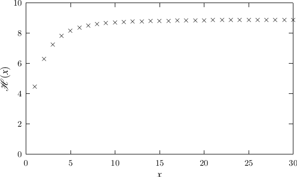
Figure 1: profile of function ℋ⁡(x)\mathcal{H}(x)
Refer to caption

3.3 numerical investigation

We turn to the numerical evaluation of the EM correction in the next-to-leading order approximation

mEM,i​j2​(L)\displaystyle m^{2}_{{\rm EM},\,ij}(L) =\displaystyle= 2​e2​CF02​(qi−qj)2+mEM,i​j2|4​(L),\displaystyle\frac{2e^{2}C}{F_{0}^{2}}\left(q_{i}-q_{j}\right)^{2}+\left.m^{2}_{{\rm EM},\,ij}\right|_{4}(L)\,, (66)

to study the qualitative features of the QED finite size scaling effect. For that purpose the values of various low energy constants found in Ref. [48] are used as reference

F0=87.7​MeV,C=4.2⋅10−5​GeV4,\displaystyle F_{0}=87.7\,{\rm MeV},\ C=4.2\cdot 10^{-5}\,{\rm GeV}^{4},
L4=0,L5=0.97⋅10−3,L6=0,L8=0.60⋅10−3,\displaystyle L_{4}=0,\ L_{5}=0.97\cdot 10^{-3},\ L_{6}=0,\ L_{8}=0.60\cdot 10^{-3},
K5=2.85⋅10−3,K9=1.3⋅10−3,K10=4.0⋅10−3,\displaystyle K_{5}=2.85\cdot 10^{-3},\ K_{9}=1.3\cdot 10^{-3},\ K_{10}=4.0\cdot 10^{-3},
K11=−1.25⋅10−3.\displaystyle K_{11}=-1.25\cdot 10^{-3}\,. (67)

The others are set to zero. We employ the formula for NS=3N_{S}=3 and NV=3N_{V}=3 and set

χ3=χ6=χ9=(500​MeV)2,\displaystyle\chi_{3}=\chi_{6}=\chi_{9}=(500\ {\rm MeV})^{2}\,,
q1=q4=q7=23,q2=q3=q5=q6=q8=q9=−13,\displaystyle q_{1}=q_{4}=q_{7}=\frac{2}{3},\,\quad q_{2}=q_{3}=q_{5}=q_{6}=q_{8}=q_{9}=-\frac{1}{3}\,, (68)

throughout the analysis. In what follows, it is always understood that the value of the mass of a ghost quark is set equal to that of the valence quark with the same flavor.

We plot the dependence of mEM, 122​(L)/mEM, 122​(∞)m^{2}_{{\rm EM},\,12}(L)/m^{2}_{{\rm EM},\,12}(\infty) on LL in Fig. 2 for the values of quark masses corresponding to χ1=χ2=χ4=χ5=(150​MeV)2\chi_{1}=\chi_{2}=\chi_{4}=\chi_{5}=(150\ {\rm MeV})^{2} and (300​MeV)2(300\ {\rm MeV})^{2}. The horizontal axis denotes the linear size of volume LL normalized in unit of 1/Mρ≃1/(770​MeV)1/M_{\rho}\simeq 1/(770\ {\rm MeV}). For instance, for the size L=16​a∼0.72×1/MρL=16\,a\sim 0.72\times 1/M_{\rho} used in Ref. [12], mEM, 122​(L)/mEM, 122​(∞)m^{2}_{{\rm EM},\,12}(L)/m^{2}_{{\rm EM},\,12}(\infty) are 0.144 and 0.421 for χ1=(150​MeV)2\chi_{1}=(150\ {\rm MeV})^{2} and χ1=(300​MeV)2\chi_{1}=(300\ {\rm MeV})^{2}, respectively. Thus, our calculation indicates that the finite size effect is significant for an available lattice geometry. The difference between two quark masses emerges for small LL, and the finite size effect is smaller for larger quark mass.

Figure 2: Linear volume size (LL) dependence of the electromagnetic correction in the charged pion mass squared
Refer to caption
Figure 3: Linear volume size (LL) dependence of the electromagnetic splitting (Δ​mK2\Delta m_{K}^{2}) in the kaon mass squared
Refer to caption

We next study the EM splitting Δ​mK2​(L)\Delta m^{2}_{{\rm K}}(L) in the (valence) kaon mass squared. Using mEM,i​j2​(L)m^{2}_{{\rm EM},\,ij}(L) in Eq. (66), it is given by

Δ​mK2​(L)\displaystyle\Delta m^{2}_{{\rm K}}(L) ≡\displaystyle\equiv mEM, 132​(L)−mEM, 232​(L).\displaystyle m^{2}_{{\rm EM},\,13}(L)-m^{2}_{{\rm EM},\,23}(L)\,. (69)

Figure 3 shows the LL-dependence of Δ​mK2​(L)/Δ​mK2​(∞)\Delta m^{2}_{{\rm K}}(L)/\Delta m^{2}_{{\rm K}}(\infty) for the two sets of quark masses corresponding to the same values of χ1=χ2=χ4=χ5\chi_{1}=\chi_{2}=\chi_{4}=\chi_{5} used in Fig. 2 with χ3=(500​MeV)2\chi_{3}=(500\ {\rm MeV})^{2} fixed. The LL-dependence in Fig. 3 is almost similar to that in Fig. 2 for each set of masses. For small LL and χ1=(150​MeV)2\chi_{1}=(150\ {\rm MeV})^{2}, the size of finite size scaling effect is smaller than the electromagnetic correction to the charged pion mass. For instance, for L=16​aL=16\,a, Δ​mK2​(L)/Δ​mK2​(∞)\Delta m^{2}_{{\rm K}}(L)/\Delta m^{2}_{{\rm K}}(\infty) is 0.2990.299 for χ1=(150​MeV)2\chi_{1}=(150\ {\rm MeV})^{2} and 0.4150.415 for χ1=(500​MeV)2\chi_{1}=(500\ {\rm MeV})^{2}. Figures 2 and 3 show that the values of EM correction depends on the quark masses for L=16​aL=16\,a. This observation indicates that the sizes of the terms depending on the quark masses in Eq. (59) are comparable to or more important than that of the term proportional to κ\kappa for the quark masses used in the present analysis.

Figure 4: Finite size scaling effect on the EM splitting (Δ​mK2\Delta m_{K}^{2}) in kaon mass squared in partially quenched QCD, where open squares stand for the LL-dependence for χ1=χ2=150​MeV\chi_{1}=\chi_{2}=150\ {\rm MeV}, χ4=χ5=300​MeV\chi_{4}=\chi_{5}=300\ {\rm MeV}, and dark squares with cross marks stand for the one for χ1=χ2=300​MeV\chi_{1}=\chi_{2}=300\ {\rm MeV}, χ4=χ5=150​MeV\chi_{4}=\chi_{5}=150\ {\rm MeV}. No significant change is observed between them. They differ from the other plots corresponding to unquenched QCD in the small volume region.
Refer to caption

Figure 4 compares the LL-dependence of the electromagnetic splitting of mK2​(L)m_{K}^{2}(L) in partially quenched QCD with that in (unquenched) QCD. The two sets of plots are drawn in Fig. 4 for

set​ 1\displaystyle{\rm set\ 1}\ ⇔\displaystyle\Leftrightarrow χ1=χ2=(150​MeV)2,χ4=χ5=(300​MeV)2,\displaystyle\ \chi_{1}=\chi_{2}=(150\ {\rm MeV})^{2},\ \chi_{4}=\chi_{5}=(300\ {\rm MeV})^{2},
set​ 2\displaystyle{\rm set\ 2} ⇔\displaystyle\Leftrightarrow χ1=χ2=(300​MeV)2,χ4=χ5=(150​MeV)2.\displaystyle\chi_{1}=\chi_{2}=(300\ {\rm MeV})^{2},\ \chi_{4}=\chi_{5}=(150\ {\rm MeV})^{2}\,. (70)

As can be seen, these two sets of plots in partially quenched QCD coincide with each other. By evaluating the LL-dependence for various set of the values of quark masses, we find that the LL-dependence for a set of the values of quark masses is almost the same as that for the set with the valence and sea quark masses interchanged. This observation together with the comparison of the relative sizes of four sets of plots in Fig. 4 shows that the size of the finite size correction is roughly determined by the average value of the quark masses involved irrespective of whether the system is unquenched or partially-quenched. To elucidate this point, we show in Figs. 5 and 6 the quark mass dependence of the finite size scaling effect on mK2​(L)m_{K}^{2}(L) on m2≡χ1=χ2=2​B0​mum^{2}\equiv\chi_{1}=\chi_{2}=2B_{0}m_{u} for fixed L=16​aL=16\,a and L=32​aL=32\,a (a≃1/(1.66​GeV)a\simeq 1/(1.66\ {\rm GeV}) [12]), respectively. In the partially quenched case, the masses of up and down sea quarks are fixed to be 300​MeV300\ {\rm MeV}. We can see that, at L=16​aL=16\,a, the size of the finite size effect changes rapidly for m2≲0.05​[GeV]2m^{2}\lesssim 0.05\ {\rm[GeV]^{2}} in the unquenched case, while no such significant change is observed in the partially quenched case. For larger m2m^{2}, they approach to each other. For L=32​aL=32\,a and larger LL, the finite size effect is determined by the relative size of LL and χ3=χ6=(500​MeV)2\chi_{3}=\chi_{6}=(500\ {\rm MeV})^{2}.

Figure 5: Dependence of the finite size scaling effect on the electromagnetic splitting (Δ​mK2\Delta m_{K}^{2}) in kaon mass squared on m2=χ1m^{2}=\chi_{1} at the tree level for L=16​aL=16\,a. The dark circular dots represent the unquenched case while the inverted triangles represent the valence quark mass dependence in partially quenched QCD.
Refer to caption
Figure 6: Dependence of the finite size scaling effect on the electromagnetic splitting (Δ​mK2\Delta m_{K}^{2}) in kaon mass squared on m2=χ1m^{2}=\chi_{1} at the tree level for L=32​aL=32\,a.
Refer to caption

4 Conclusion and discussion

In this paper, we studied the finite size scaling effect on the electromagnetic (EM) correction to the pseudoscalar meson masses from the low energy effective field theory of QCD including electromagnetism. For that purpose, we began with constructing a new QED in finite volume, QEDL. Taking the practical application to the lattice simulation into account, we adapted it to the partially quenched chiral perturbation theory including electromagnetism. We computed the electromagnetic correction to the pseudoscalar meson mass squared at the next-to-leading order on both of the spaces with finite and infinite volumes for generic number NSN_{S} of sea quarks. Through numerical investigation for NS=3N_{S}=3, we found that the finite size scaling effect on the EM correction is sizable on the space with the volume available in the lattice simulation. By investigating its dependence on the quark masses in unquenched and partially quenched systems, we pointed out that the finite size correction is determined by the averaged values of masses of quarks involved in the system. Though the current study was restricted to the pseudoscalar meson masses, we can study the EM corrections to the other hadronic observables such as decay constants in finite volume.

It should be noted that the finite size correction tends to increase for the increase of the extent TT of the temporal direction. For example, let us suppose that the value ∼0.9\sim 0.9 in Eq. (4) does not change so drastically even if the contribution of A~μ​(t, 0)\widetilde{A}_{\mu}(t,\,{\bf 0}) is subtracted. The explicit calculation in the low energy effective theory including vector and axial-vector mesons show that it is reduced to about 0.60.6 in the limit T→∞T\rightarrow\infty. Since the simulation has to be performed with finite TT, mEM, 122​(L)/mEM, 122​(∞)m^{2}_{{\rm EM},\,12}(L)/m^{2}_{{\rm EM},\,12}(\infty) obtained in our present analysis with T→∞T\rightarrow\infty may overestimate the finite size correction in the actual simulation. It is one of the subjects to fill the gap between these two.

Finally, we recall that we construct QEDL because we would like to respect the boundary condition (i.e., periodic boundary condition) for the meson fields along spatial directions usually assumed in the lattice QCD simulations, and to understand the qualitative properties of the finite size scaling effect with the practical situation in our mind. It is plausible that the finite size scaling effect depends on the boundary conditions imposed on fields. As illustrated in Figs. 4, if periodic boundary condition is employed, the dependence on the volume is not simple around the available volume L⋅(0.77​GeV)≲10L\cdot(0.77\ {\rm GeV})\lesssim 10 in the lattice simulations. It would be one of the important subjects to study the finite size scaling effect on EM corrections for the various types of boundary conditions and to select the one in which the finite size effect exhibits such a simplest behavior that allows us to extrapolate the data at available volumes to the value in infinite volume.

Acknowledgments.
We thank T. Blum, T. Doi, T. Izubuchi, N. Yamada, K. Yamawaki and R. Zhou for valuable discussions. This work is supported in part by JSPS Grant-in-Aid for Scientific Research (C) 20540261 and MEXT Grant-in-Aid for Scientific Research on Priority Areas “Higgs and Supersymmetry” 20025010.

Appendix A Formulae for several sums

The one-loop corrections to meson masses in chiral perturbation theory for QCD plus QED system with finite volume are described in terms of several basic functions. Each of these functions takes the form of the one-dimensional integral of the sum over three-dimensional momenta of some function. We employ dimensional regularization and define

∫−∞∞d​k02​π​i1V∑𝐤∈Γ~d=0.\displaystyle\displaystyle{\int_{-\infty}^{\infty}\frac{dk^{0}}{2\pi i}\,\frac{1}{V}\sum_{{\bf k}\in\widetilde{\Gamma}_{d}}=0\,.} (71)

Here, d≡D−1d\equiv D-1, V≡LdV\equiv L^{d} and the sum runs over all 𝐤∈Γ~d{\bf k}\in\widetilde{\Gamma}_{d}, where

Γ~d≡{𝐤=(k1,⋯,kd)|kj∈2​πLℤ}.\displaystyle\displaystyle{\widetilde{\Gamma}_{d}\equiv\left\{{\bf k}=\left(k^{1},\,\cdots,\,k^{d}\right)\,\left|\,k^{j}\in\frac{2\pi}{L}\,\mathbb{Z}\right.\right\}\,.} (72)

The aim of this Appendix is to get compact expressions for the four functions that can be evaluated by MATHEMATICA and so forth by following the strategy in Ref. [23].

We first consider the function

I11​(m2,L)≡(μ2)2−D2​∫−∞∞d​k02​π​i​1V​∑𝐤∈Γ~d′1(−k2−i​ϵ)​{m2−(k+p)2−i​ϵ}.\displaystyle\displaystyle{I_{11}(m^{2};\,L)\equiv\left(\mu^{2}\right)^{2-\frac{D}{2}}\int_{-\infty}^{\infty}\frac{dk^{0}}{2\pi i}\frac{1}{V}\sum_{{\bf k}\in\widetilde{\Gamma}_{d}^{\prime}}\frac{1}{\left(-k^{2}-i\epsilon\right)\left\{m^{2}-\left(k+p\right)^{2}-i\epsilon\right\}}\,.} (73)

In the above, pp is assumed to be on-shell, p2=m2p^{2}=m^{2} and Γ~d′≡Γ~d−{𝟎}\widetilde{\Gamma}_{d}^{\prime}\equiv\widetilde{\Gamma}_{d}-\left\{{\bf 0}\right\}.

By introducing the Feynman parameters as usual, Eq. (73) becomes

I11​(m2,L)≡∫01d​y​∫−∞∞d​k02​π​i​1V​∑𝐤∈Γ~d′1{y2​m2−(k+y​p)2−i​ϵ}2,\displaystyle\displaystyle{I_{11}(m^{2};\,L)\equiv\int_{0}^{1}dy\int_{-\infty}^{\infty}\frac{dk^{0}}{2\pi i}\frac{1}{V}\sum_{{\bf k}\in\widetilde{\Gamma}_{d}^{\prime}}\frac{1}{\left\{y^{2}m^{2}-(k+yp)^{2}-i\epsilon\right\}^{2}}\,,} (74)

The sum of a function F~​(𝐤)\widetilde{F}({\bf k}) over 𝐤∈Γ~d′{\bf k}\in\widetilde{\Gamma}_{d}^{\prime} can be written as an integral

1V​∑𝐤∈Γ~d′F~​(𝐤)=∫dd​k′​F~​(𝐤′)​1V​∑𝐤∈Γ~dδd​(𝐤′−𝐤)−1V​F~​(𝟎).\displaystyle\displaystyle{\frac{1}{V}\sum_{{\bf k}\in\widetilde{\Gamma}_{d}^{\prime}}\widetilde{F}({\bf k})=\int d^{d}k^{\prime}\widetilde{F}({\bf k}^{\prime})\,\frac{1}{V}\sum_{{\bf k}\in\widetilde{\Gamma}_{d}}\delta^{d}\left({\bf k}^{\prime}-{\bf k}\right)-\frac{1}{V}\,\widetilde{F}({\bf 0})\,.} (75)

Using the Poisson resummation

1V​∑𝐤∈Γ~dδd​(𝐤′−𝐤)=1(2​π)d​∑𝐱∈Γdei​𝐤⋅𝐱,\displaystyle\displaystyle{\frac{1}{V}\sum_{{\bf k}\in\widetilde{\Gamma}_{d}}\delta^{d}\left({\bf k}^{\prime}-{\bf k}\right)=\frac{1}{\left(2\pi\right)^{d}}\sum_{{\bf x}\in\Gamma_{d}}e^{i{\bf k}\cdot{\bf x}}\,,} (76)

where

Γd≡{𝐱≡(x1,⋯,xd)|xj∈Lℤ},\displaystyle\displaystyle{\Gamma_{d}\equiv\left\{{\bf x}\equiv\left(x^{1},\,\cdots,\,x^{d}\right)\,\left|x^{j}\in L\mathbb{Z}\right.\right\}\,,} (77)

the sum (75) can be written as

1V​∑𝐤∈Γ~d′F~​(𝐤)=∑𝐱∈ΓdF⁡(𝐱)−1V​∫dd​x​F​(𝐱),\displaystyle\displaystyle{\frac{1}{V}\sum_{{\bf k}\in\widetilde{\Gamma}_{d}^{\prime}}\widetilde{F}({\bf k})=\sum_{{\bf x}\in\Gamma_{d}}F({\bf x})-\frac{1}{V}\,\int d^{d}x\,F({\bf x})\,,} (78)

where F⁡(𝐱)F({\bf x}) is obtained by Fourier transformation of F~​(𝐤)\widetilde{F}({\bf k})

F⁡(𝐱)=∫dd​k(2​π)d​ei​𝐤⋅𝐱​F~​(𝐤).\displaystyle\displaystyle{F({\bf x})=\int\frac{d^{d}k}{\left(2\pi\right)^{d}}\,e^{i{\bf k}\cdot{\bf x}}\,\widetilde{F}({\bf k})\,.} (79)

In the present context F~​(𝐤)\widetilde{F}({\bf k}) is

F~​(𝐤)\displaystyle\widetilde{F}({\bf k}) =\displaystyle= 1{y2​m2−(k+y​p)2−i​ϵ}2\displaystyle\frac{1}{\left\{y^{2}m^{2}-\left(k+yp\right)^{2}-i\epsilon\right\}^{2}} (80)
=\displaystyle= 1Γ⁡(2)​∫0∞d​λλ​(i​λ)2​exp⁡[−i​λ​{y2​m2−(k+z​p)2−i​ϵ}].\displaystyle\frac{1}{\Gamma(2)}\int_{0}^{\infty}\frac{d\lambda}{\lambda}\left(i\lambda\right)^{2}\exp\left[-i\lambda\left\{y^{2}m^{2}-\left(k+zp\right)^{2}-i\epsilon\right\}\right]\,.

A given dd-dimensional vector 𝐱{\bf x} defines a DD-dimensional space-like vector xμ=(0,𝐱)x^{\mu}=(0,\,{\bf x}). A one-dimensional integral in Eq. (74) and a dd-dimension integral in Eq. (79) combine to become an integral over DD-dimensional momenta, which can be readily carried out;

∫0∞d​λλ​(i​λ)2​∫dD​ki​(2​π)D​exp⁡[−i​λ​{−(k+y​p)2−i​ϵ}−i​x⋅k]\displaystyle\int_{0}^{\infty}\frac{d\lambda}{\lambda}\left(i\lambda\right)^{2}\int\frac{d^{D}k}{i\left(2\pi\right)^{D}}\exp\left[-i\lambda\left\{-\left(k+yp\right)^{2}-i\epsilon\right\}-ix\cdot k\right]
=∫0∞d​λλ​λ2(4​π​λ)D2​exp⁡[−λ⁡{(i​x2​λ−y​p)2−(y​p)2}].\displaystyle\quad=\int_{0}^{\infty}\frac{d\lambda}{\lambda}\frac{\lambda^{2}}{\left(4\pi\lambda\right)^{\frac{D}{2}}}\exp\left[-\lambda\left\{\left(i\frac{x}{2\lambda}-yp\right)^{2}-(yp)^{2}\right\}\right]\,. (81)

For pμ=(m, 0)p^{\mu}=(m,\,{\bf 0}), (i​x2​λ−y​p)2−(y​p)2=|𝐱|24​λ2\left(i\frac{x}{2\lambda}-yp\right)^{2}-(yp)^{2}=\frac{\left|{\bf x}\right|^{2}}{4\lambda^{2}}. Eq. (74) thus becomes

I11​(m2,L)\displaystyle I_{11}(m^{2};\,L) =\displaystyle= (μ2)2−D2∫01dy(∑𝐧∈ℤd−∫ddn)\displaystyle\left(\mu^{2}\right)^{2-\frac{D}{2}}\int_{0}^{1}dy\left(\sum_{{\bf n}\in\mathbb{Z}^{d}}-\int d^{d}n\right) (82)
×∫0∞d​λλ​λ2(4​π​λ)D2​exp⁡(−λ​y2​m2−L24​λ​|𝐧|2).\displaystyle\quad\times\int_{0}^{\infty}\frac{d\lambda}{\lambda}\,\frac{\lambda^{2}}{\left(4\pi\lambda\right)^{\frac{D}{2}}}\,\exp\left(-\lambda\,y^{2}m^{2}-\frac{L^{2}}{4\lambda}\left|{\bf n}\right|^{2}\right)\,.

In the sum appearing above, the contribution of 𝐧=𝟎{\bf n}={\bf 0} is exactly I11(m2)=I11(m2;L→∞)I_{11}(m^{2})=I_{11}(m^{2};\,L\rightarrow\infty). I11​(m2,L)−I11​(m2)I_{11}(m^{2};\,L)-I_{11}(m^{2}) is hence free of UV divergence. Letting D→4D\rightarrow 4 for this difference and rescaling λ→L24​π​λ\lambda\rightarrow\frac{L^{2}}{4\pi}\lambda leads

I11​(m2,L)−I11​(m2)=−116​π2​1m​L​ℋ​(m​L).\displaystyle I_{11}(m^{2};\,L)-I_{11}(m^{2})=-\frac{1}{16\pi^{2}}\,\frac{1}{mL}\,\mathcal{H}(mL)\,. (83)

Here

ℋ⁡(m​L)\displaystyle\mathcal{H}(mL) ≡\displaystyle\equiv π​∫0∞d​λλ32​erf​(m​L​λ4​π)​𝒮​(λ),\displaystyle\pi\int_{0}^{\infty}\frac{d\lambda}{\lambda^{\frac{3}{2}}}\,{\rm erf}\left(mL\sqrt{\frac{\lambda}{4\pi}}\right)\mathcal{S}(\lambda)\,, (84)
𝒮⁡(λ)\displaystyle\mathcal{S}(\lambda) ≡\displaystyle\equiv −(∑𝐧∈𝒵3−{𝟎}−∫d3n)exp(−πλ|𝐧|2)\displaystyle-\left(\sum_{{\bf n}\in\mathcal{Z}^{3}-\left\{{\bf 0}\right\}}-\int d^{3}n\right)\exp\left(-\frac{\pi}{\lambda}\left|{\bf n}\right|^{2}\right) (85)
=\displaystyle= −{(ϑ3​(0,i​1λ))3−1−λ32},\displaystyle-\left\{\left(\vartheta_{3}\left(0,\,i\frac{1}{\lambda}\right)\right)^{3}-1-\lambda^{\frac{3}{2}}\right\}\,,

where erf⁡(x){\rm erf}(x) is the error function

erf⁡(x)=2π​∫0xd​s​e−s2,\displaystyle\displaystyle{{\rm erf}(x)=\frac{2}{\sqrt{\pi}}\int_{0}^{x}ds\,e^{-s^{2}}\,,} (86)

and ϑ3​(v,τ)\vartheta_{3}(v;\,\tau) is a Jacobi-theta function

ϑ3​(v,τ)=∑n=−∞∞exp⁡(π​τ​i​n2+2​π​v​i​n).\displaystyle\vartheta_{3}(v;\,\tau)=\sum_{n=-\infty}^{\infty}\exp\left(\pi\tau in^{2}+2\pi vin\right)\,. (87)

We recall that the term λ32\lambda^{\frac{3}{2}} in 𝒮⁡(λ)\mathcal{S}(\lambda) arises in our new QED, QEDL. Because

ϑ3​(0,i​1λ)→λ12,\displaystyle\vartheta_{3}\left(0,\,i\,\frac{1}{\lambda}\right)\rightarrow\lambda^{\frac{1}{2}}\,, (88)

in the infrared limit λ→∞\lambda\rightarrow\infty, the presence of that term indeed ensures IR-finiteness of the integral over λ\lambda in the expression (84). The numerical study shows that

limx→0ℋ⁡(x)x≃10.4.\displaystyle\lim_{x\rightarrow 0}\frac{\mathcal{H}(x)}{x}\simeq 10.4\,. (89)

Next we consider the function

J11​(m2,L)≡(μ2)2−D2​∫−∞∞d​k02​π​i​1V​∑𝐤∈Γ~d′p⋅k(−k2−i​ϵ)​{m2−(k+p)2−i​ϵ}.\displaystyle\displaystyle{J_{11}(m^{2};\,L)\equiv\left(\mu^{2}\right)^{2-\frac{D}{2}}\int_{-\infty}^{\infty}\frac{dk^{0}}{2\pi i}\frac{1}{V}\sum_{{\bf k}\in\widetilde{\Gamma}_{d}^{\prime}}\frac{p\cdot k}{\left(-k^{2}-i\epsilon\right)\left\{m^{2}-\left(k+p\right)^{2}-i\epsilon\right\}}\,.}
(90)

The same manipulation as done for I11​(m2,L)I_{11}(m^{2};\,L) in Eq. (80) leads

J11​(m2,L)\displaystyle J_{11}(m^{2};\,L) =\displaystyle= ∫01dy(∑𝐱∈Γd−1V∫ddx)\displaystyle\int_{0}^{1}dy\left(\sum_{{\bf x}\in\Gamma_{d}}-\frac{1}{V}\int d^{d}x\right) (91)
×1Γ⁡(2)​∫0∞d​λλ​(i​λ)2​(μ2)2−D2​∫dD​ki​(2​π)D\displaystyle\ \times\frac{1}{\Gamma(2)}\int_{0}^{\infty}\frac{d\lambda}{\lambda}\left(i\lambda\right)^{2}\left(\mu^{2}\right)^{2-\frac{D}{2}}\int\frac{d^{D}k}{i\left(2\pi\right)^{D}}
×p⋅k​exp⁡[−(i​λ)​{y2​m2−(k+y​p)2−i​ϵ}−i​x⋅k].\displaystyle\ \times p\cdot k\exp\left[-(i\lambda)\left\{y^{2}m^{2}-\left(k+yp\right)^{2}-i\epsilon\right\}-ix\cdot k\right]\,.

We follow Appendix of Ref. [49] to carry out such integrals with kμk_{\mu} in the numerator. We replace kμk_{\mu} appearing in the numerator as

kμ=[−121i​λ∂∂ρμexp(−2(iλ)ρ⋅k)]ρ→0.\displaystyle\displaystyle{k_{\mu}=\left[-\frac{1}{2}\,\frac{1}{i\lambda}\,\frac{\partial}{\partial\rho^{\mu}}\exp\left(-2\left(i\lambda\right)\rho\cdot k\right)\right]_{\rho\rightarrow 0}\,.} (92)

Carrying out the integral of kk and performing a ρ\rho-derivative gives

J11​(m2,L)\displaystyle J_{11}(m^{2};\,L) =\displaystyle= ∫01dy(∑𝐱∈Γd−1V∫ddx)∫0∞d​λλλ2(4​π​λ)D2\displaystyle\int_{0}^{1}dy\left(\sum_{{\bf x}\in\Gamma_{d}}-\frac{1}{V}\int d^{d}x\right)\int_{0}^{\infty}\frac{d\lambda}{\lambda}\frac{\lambda^{2}}{\left(4\pi\lambda\right)^{\frac{D}{2}}}
×p⋅(i​x2​λ−y​p)​exp⁡[−λ​(i​x2​λ−y​p)2]\displaystyle\quad\times p\cdot\left(i\,\frac{x}{2\lambda}-yp\right)\exp\left[-\lambda\left(i\,\frac{x}{2\lambda}-yp\right)^{2}\right]
=\displaystyle= −12(∑𝐱∈Γd−1V∫ddx)∫0∞d​λλλ(4​π​λ)D2(1−e−λ​m2)e−|𝐱|24​λ,\displaystyle-\frac{1}{2}\left(\sum_{{\bf x}\in\Gamma_{d}}-\frac{1}{V}\int d^{d}x\right)\int_{0}^{\infty}\frac{d\lambda}{\lambda}\frac{\lambda}{\left(4\pi\lambda\right)^{\frac{D}{2}}}\left(1-e^{-\lambda m^{2}}\right)e^{-\frac{\left|{\bf x}\right|^{2}}{4\lambda}}\,,

where the second equality follows by taking pμ=(m, 0)p^{\mu}=(m,\,{\bf 0}) and performing the integral over yy. In Eq. (), UV divergence is contained in the term with 𝐱=𝟎{\bf x}={\bf 0}, which is exactly J11(m2)=J11(m2,L→∞)J_{11}(m^{2})=J_{11}(m^{2},\,L\rightarrow\infty). Therefore, J11​(m2,L)−J11​(m2)J_{11}(m^{2};\,L)-J_{11}(m^{2}) is UV-finite. In terms of the function

𝒦⁡(x)≡4​π​∫0∞d​λλ​1λ​(1−e−x24​π​λ)​𝒮​(λ),\displaystyle\displaystyle{\mathcal{K}(x)\equiv 4\pi\int_{0}^{\infty}\frac{d\lambda}{\lambda}\,\frac{1}{\lambda}\left(1-e^{-\frac{x^{2}}{4\pi}\,\lambda}\right)\mathcal{S}(\lambda)\,,} (94)

it can be expressed as

J11​(m2,L)−J11​(m2)\displaystyle J_{11}(m^{2};\,L)-J_{11}(m^{2}) =\displaystyle= 132​π2​1L2​𝒦​(m​L).\displaystyle\frac{1}{32\pi^{2}}\,\frac{1}{L^{2}}\,\mathcal{K}(mL)\,. (95)

The quantity

I10​(L)\displaystyle I_{1}^{0}(L) ≡\displaystyle\equiv (μ2)2−D2​∫−∞∞d​k02​π​i​1V​∑𝐤∈Γ~d′1−k2−i​ϵ,\displaystyle\left(\mu^{2}\right)^{2-\frac{D}{2}}\int_{-\infty}^{\infty}\frac{dk^{0}}{2\pi i}\frac{1}{V}\sum_{{\bf k}\in\widetilde{\Gamma}_{d}^{\prime}}\frac{1}{-k^{2}-i\epsilon}\,, (96)

needs a special care. In dimensional regularization, we put

I10​(∞)=(μ2)2−D2​∫dD​ki​(2​π)D​1−k2−i​ϵ=0.\displaystyle\displaystyle{I_{1}^{0}(\infty)=\left(\mu^{2}\right)^{2-\frac{D}{2}}\int\frac{d^{D}k}{i\left(2\pi\right)^{D}}\,\frac{1}{-k^{2}-i\epsilon}=0\,.}

However, we cannot set I10​(L)=0I_{1}^{0}(L)=0. For instance, if the integral

(μ2)2−D2​∫−∞∞d​k02​π​i​1Ld​∑𝐤∈Γ~d′1(−k2−i​ϵ)​(m2−k2−i​ϵ)\displaystyle\left(\mu^{2}\right)^{2-\frac{D}{2}}\int_{-\infty}^{\infty}\frac{dk^{0}}{2\pi i}\frac{1}{L^{d}}\sum_{{\bf k}\in\widetilde{\Gamma}_{d}^{\prime}}\frac{1}{\left(-k^{2}-i\epsilon\right)\left(m^{2}-k^{2}-i\epsilon\right)}
=1m2​(μ2)2−D2​∫−∞∞d​k02​π​i​1Ld​∑𝐤∈Γ~d′(1−k2−i​ϵ−1m2−k2−i​ϵ),\displaystyle\qquad=\frac{1}{m^{2}}\left(\mu^{2}\right)^{2-\frac{D}{2}}\int_{-\infty}^{\infty}\frac{dk^{0}}{2\pi i}\frac{1}{L^{d}}\sum_{{\bf k}\in\widetilde{\Gamma}_{d}^{\prime}}\left(\frac{1}{-k^{2}-i\epsilon}-\frac{1}{m^{2}-k^{2}-i\epsilon}\right)\,, (97)

were evaluated in two different ways; (1) direct evaluation of the left-hand side by introducing a Feynman parameter, and (2) evaluation of the right-hand only with the second term kept, inconsistency would arise. A straightforward calculation yields

I10​(L)−I10​(∞)=−κ4​π​1L2,\displaystyle\displaystyle{I_{1}^{0}(L)-I_{1}^{0}(\infty)=-\frac{\kappa}{4\pi}\,\frac{1}{L^{2}}\,,} (98)

where κ\kappa is a constant defined by

κ≡∫0∞d​λλ2​𝒮​(λ)≊2.837.\displaystyle\displaystyle{\kappa\equiv\int_{0}^{\infty}\frac{d\lambda}{\lambda^{2}}\,\mathcal{S}(\lambda)\approxeq 2.837\,.} (99)

All the one-loop contributions induced by quartic couplings are described by a function

I1​(m2,L)\displaystyle I_{1}(m^{2};\,L) ≡\displaystyle\equiv (μ2)2−D2​∫−∞∞d​k02​π​i​1V​∑𝐤∈Γ~d1m2−k2−i​ϵ.\displaystyle\left(\mu^{2}\right)^{2-\frac{D}{2}}\int_{-\infty}^{\infty}\frac{dk^{0}}{2\pi i}\frac{1}{V}\sum_{{\bf k}\in\widetilde{\Gamma}_{d}}\frac{1}{m^{2}-k^{2}-i\epsilon}\,. (100)

The expression for I1​(m2,L)I_{1}(m^{2};\,L) in terms of Jacobi-theta function was obtained in Ref. [23]

I1​(m2,L)−I1​(m2)\displaystyle I_{1}(m^{2};\,L)-I_{1}(m^{2}) =\displaystyle= 1(4​π)2​ℳ⁡(m​L)L2,\displaystyle\frac{1}{\left(4\pi\right)^{2}}\,\frac{\mathcal{M}(mL)}{L^{2}}\,, (101)

where

ℳ⁡(x)\displaystyle\mathcal{M}(x) ≡\displaystyle\equiv 4​π​∫0∞d​λλ2​exp⁡(−x24​π​λ)​𝒯​(λ),\displaystyle 4\pi\int_{0}^{\infty}\frac{d\lambda}{\lambda^{2}}\,\exp\left(-\frac{x^{2}}{4\pi}\,\lambda\right)\mathcal{T}(\lambda)\,, (102)

and

𝒯⁡(λ)\displaystyle\mathcal{T}(\lambda) ≡\displaystyle\equiv ∑𝐧∈(ℤ3−{𝟎})exp⁡(−πλ​|𝐧|2)\displaystyle\sum_{{\bf n}\in\left(\mathbb{Z}^{3}-\left\{{\bf 0}\right\}\right)}\exp\left(-\frac{\pi}{\lambda}\,\left|{\bf n}\right|^{2}\right) (103)
=\displaystyle= (θ3​(0,i​1λ))3−1.\displaystyle\left(\theta_{3}\left(0,\,i\,\frac{1}{\lambda}\right)\right)^{3}-1\,.

References

  • [1] CP-PACS Collaboration, A. Ali Khan et. al., Light hadron spectroscopy with two flavors of dynamical quarks on the lattice, Phys. Rev. D 65 (2002) 054505, [hep-lat/0105015].
  • [2] JLQCD Collaboration, S. Aoki et. al., Light hadron spectroscopy with two flavors of O⁡(a)O(a)-improved dynamical quarks, Phys. Rev. D 68 (2003) 054502, [hep-lat/0212039].
  • [3] QCDSF Collaboration, M. Gockeler et. al., Determination of light and strange quark masses from full lattice QCD, Phys. Lett. B639 (2006) 307–311, [hep-ph/0409312].
  • [4] ALPHA Collaboration, M. Della Morte et. al., Non-perturbative quark mass renormalization in two-flavor QCD, Nucl. Phys. B729 (2005) 117–134, [hep-lat/0507035].
  • [5] D. Becirevic et. al., Non-perturbatively renormalised light quark masses from a lattice simulation with Nf=2N_{f}=2, Nucl. Phys. B734 (2006) 138–155, [hep-lat/0510014].
  • [6] European Twisted Mass Collaboration, B. Blossier et. al., Light quark masses and pseudoscalar decay constants from Nf=2N_{f}=2 Lattice QCD with twisted mass fermions, arXiv:0709.4574.
  • [7] HPQCD Collaboration, C. Aubin et. al., First determination of the strange and light quark masses from full lattice QCD, Phys. Rev. D 70 (2004) 031504, [hep-lat/0405022].
  • [8] MILC Collaboration, C. Aubin et. al., Light pseudoscalar decay constants, quark masses, and low energy constants from three-flavor lattice QCD, Phys. Rev. D 70 (2004) 114501, [hep-lat/0407028].
  • [9] HPQCD Collaboration, Q. Mason, H. D. Trottier, R. Horgan, C. T. H. Davies, and G. P. Lepage, High-precision determination of the light-quark masses from realistic lattice QCD, Phys. Rev. D 73 (2006) 114501, [hep-ph/0511160].
  • [10] JLQCD Collaboration, T. Ishikawa et. al., Light quark masses from unquenched lattice QCD, arXiv:0704.1937.
  • [11] A. Duncan, E. Eichten, and H. Thacker, Electromagnetic Splittings and Light Quark Masses in Lattice QCD, Phys. Rev. Lett. 76 (1996) 3894–3897, [hep-lat/9602005].
  • [12] T. Blum, T. Doi, M. Hayakawa, T. Izubuchi, and N. Yamada, Determination of light quark masses from the electromagnetic splitting of pseudoscalar meson masses computed with two flavors of domain wall fermions, Phys. Rev. D 76 (2007) 114508, [arXiv:0708.0484].
  • [13] Y. Namekawa and Y. Kikukawa, Electromagnetic mass difference on the lattice, PoS LAT2005 (2006) 090, [hep-lat/0509120].
  • [14] JLQCD Collaboration, E. Shintani et. al., Pion mass difference from vacuum polarization, PoS LAT2007 (2007) 134, [arXiv:0710.0691].
  • [15] T. Das, G. S. Guralnik, V. S. Mathur, F. E. Low, and J. E. Young, Electromagnetic mass difference of pions, Phys. Rev. Lett. 18 (1967) 759–761.
  • [16] M. Luscher, On a relation between finite size effects and elastic scattering processes, . Lecture given at Cargese Summer Inst., Cargese, France, Sep 1-15, 1983.
  • [17] M. Luscher, Volume Dependence of the Energy Spectrum in Massive Quantum Field Theories. 1. Stable Particle States, Commun. Math. Phys. 104 (1986) 177.
  • [18] M. Luscher, Volume Dependence of the Energy Spectrum in Massive Quantum Field Theories. 2. Scattering States, Commun. Math. Phys. 105 (1986) 153–188.
  • [19] J. Gasser and H. Leutwyler, Spontaneously Broken Symmetries: Eeffective Lagrangians at Finite Volume, Nucl. Phys. B307 (1988) 763.
  • [20] P. Hasenfratz and H. Leutwyler, Goldstone boson related finite size effects in field theory and critical phenomena with O⁡(N)O(N) symmetry, Nucl. Phys. B343 (1990) 241–284.
  • [21] F. C. Hansen, Finite size effects in spontaneously broken S​U​(N)×S​U​(N)SU(N)\times SU(N) theories, Nucl. Phys. B345 (1990) 685–708.
  • [22] G. Colangelo and S. Durr, The pion mass in finite volume, Eur. Phys. J. C 33 (2004) 543–553, [hep-lat/0311023].
  • [23] QCDSF-UKQCD Collaboration, A. Ali Khan et. al., The nucleon mass in NF=2N_{F}=2 lattice QCD: Finite size effects from chiral perturbation theory, Nucl. Phys. B689 (2004) 175–194, [hep-lat/0312030].
  • [24] Y. Koma and M. Koma, On the finite size mass shift formula for stable particles, Nucl. Phys. B713 (2005) 575–597, [hep-lat/0406034].
  • [25] G. Colangelo, Finite volume effects in chiral perturbation theory, Nucl. Phys. Proc. Suppl. 140 (2005) 120–126, [hep-lat/0409111].
  • [26] G. Colangelo, S. Durr, and C. Haefeli, Finite volume effects for meson masses and decay constants, Nucl. Phys. B721 (2005) 136–174, [hep-lat/0503014].
  • [27] I. Caprini, G. Colangelo, and H. Leutwyler, Mass and width of the lowest resonance in QCD, Phys. Rev. Lett. 96 (2006) 132001, [hep-ph/0512364].
  • [28] G. Colangelo and C. Haefeli, Finite volume effects for the pion mass at two loops, Nucl. Phys. B744 (2006) 14–33, [hep-lat/0602017].
  • [29] W. A. Bardeen, J. Bijnens, and J. M. Gerard, Hadronic Matrix Elements and the π+\pi^{+}-π0\pi^{0} Mass Difference, Phys. Rev. Lett. 62 (1989) 1343.
  • [30] G. Ecker, J. Gasser, A. Pich, and E. de Rafael, The Role of Resonances in Chiral Perturbation Theory, Nucl. Phys. B321 (1989) 311.
  • [31] R. Urech, Virtual photons in chiral perturbation theory, Nucl. Phys. B433 (1995) 234–254, [hep-ph/9405341].
  • [32] M. Knecht and R. Urech, Virtual photons in low energy π\pi-π\pi scattering, Nucl. Phys. B519 (1998) 329–360, [hep-ph/9709348].
  • [33] J. Bijnens and N. Danielsson, Electromagnetic corrections in partially quenched chiral perturbation theory, Phys. Rev. D 75 (2007) 014505, [hep-lat/0610127].
  • [34] C. Haefeli, M. A. Ivanov, and M. Schmid, Electromagnetic low-energy constants in ChPT, Eur. Phys. J. C 53 (2008) 549–557, [0710.5432].
  • [35] J. Gasser, A. Rusetsky, and I. Scimemi, Electromagnetic corrections in hadronic processes, Eur. Phys. J. C32 (2003) 97–114, [hep-ph/0305260].
  • [36] C. W. Bernard and M. F. L. Golterman, Chiral perturbation theory for the quenched approximation of QCD, Phys. Rev. D 46 (1992) 853–857, [hep-lat/9204007].
  • [37] S. R. Sharpe, Quenched chiral logarithms, Phys. Rev. D 46 (1992) 3146–3168, [hep-lat/9205020].
  • [38] S. R. Sharpe and N. Shoresh, Physical results from unphysical simulations, Phys. Rev. D 62 (2000) 094503, [hep-lat/0006017].
  • [39] S. R. Sharpe and N. Shoresh, Partially quenched chiral perturbation theory without Φ0\Phi_{0}, Phys. Rev. D 64 (2001) 114510, [hep-lat/0108003].
  • [40] M. Henneaux and C. Teitelboim, Quantization of gauge systems, . Princeton University Presse, New Jersey (1992), 520 p.
  • [41] T. Filk, Divergencies in a field theory on quantum space, Phys. Lett. B376 (1996) 53–58.
  • [42] S. Minwalla, M. Van Raamsdonk, and N. Seiberg, Noncommutative perturbative dynamics, JHEP 02 (2000) 020, [hep-th/9912072].
  • [43] M. Hayakawa, Perturbative analysis on infrared aspects of noncommutative QED on ℝ4\mathbb{R}^{4}, Phys. Lett. B478 (2000) 394–400, [hep-th/9912094].
  • [44] J. Bijnens, Chiral perturbation theory beyond one loop, Prog. Part. Nucl. Phys. 58 (2007) 521–586, [hep-ph/0604043].
  • [45] J. Gasser and H. Leutwyler, Chiral Perturbation Theory to One Loop, Ann. Phys. 158 (1984) 142.
  • [46] J. Gasser and H. Leutwyler, Chiral Perturbation Theory: Expansions in the Mass of the Strange Quark, Nucl. Phys. B250 (1985) 465.
  • [47] J. Bijnens, G. Colangelo, and G. Ecker, Renormalization of chiral perturbation theory to order p6p^{6}, Annals Phys. 280 (2000) 100–139, [hep-ph/9907333].
  • [48] J. Bijnens and J. Prades, Electromagnetic corrections for pions and kaons: Masses and polarizabilities, Nucl. Phys. B490 (1997) 239–271, [hep-ph/9610360].
  • [49] M. Hayakawa, Perturbative analysis on infrared and ultraviolet aspects of noncommutative QED on ℝ4\mathbb{R}^{4}, hep-th/9912167.