Particle creation in the presence of a warped extra dimension
Abstract
Particle creation in spacetimes with a warped extra dimension is studied. In particular, we investigate the dynamics of a conformally coupled, massless scalar field in a five dimensional warped geometry where the induced metric on the 3–branes is that of a spatially flat cosmological model. We look at situations where the scale of the extra dimension is assumed (i) to be time independent or (ii) to have specific functional forms for time dependence. The warp factor is chosen to be that of the Randall–Sundrum model. With particular choices for the functional form of the scale factor (and also the function characterising the time evolution of the extra dimension) we obtain the , the particle number and energy densities after solving (wherever possible, analytically but, otherwise, numerically) the conformal scalar field equations. The behaviour of these quantities for the massless and massive Kaluza–Klein modes are examined. Our results show the effect of a warped extra dimension on particle creation and illustrate how the nature of particle production on the brane depends on the nature of warping, type of cosmological evolution as well as the temporal evolution of the extra dimension.
pacs
04.62.+v, 04.50.-h, 11.10.KkI Introduction
Beginning with Kaluza-Klein [1], a large variety of models with extra dimensions have been proposed over the years. The recent brane-world models [2]-[5] where our world is viewed as a four dimensional sub-manifold (3-brane) embedded in five dimensions are actively pursued today largely because of their potential in proposing achievable experimental signatures of extra dimensions. Among braneworld models, the warped type necessarily assumes a curved higher dimensional spacetime and the line element on the 3–brane is scaled by a warp factor, thereby rendering the higher dimensional metric non-factorisable. The brane-world models seem to provide a viable resolution of the long-standing hierarchy problem in high energy physics. The warped braneworlds also suggest a dynamic way of compactification by proposing the idea of localisation of fields on the brane [6] (and references therein).
A study of quantum field theory in the context of warped spacetimes where there is an extra dimension is therefore not inappropriate. However, not much has been done along this direction. Leaving aside warping, the analysis of quantum field theory in a higher dimensional spacetime with a Kaluza–Klein-like extra dimension has been discussed by some–notable among them being the works reported in [7], [8], [9], [10]. More recently, Saharian [11] (and references therein) has discussed quantum fields in such spacetimes quite extensively (though, somewhat on the formal side) in a series of papers. Gravitational particle production in braneworld cosmology and its implications have been studied in [12].
The questions we address in this article are the following. Particle creation in a cosmological background spacetime using the formalism of quantum fields in curved spacetime [13] is a well–studied subject. How do the presence of extra dimensions affect particle creation? Further, how does a warping of the higher dimensional spacetime create differences, if any. The simple answer to the first question is related to the fact that now we do not refer to but we must consider , where is the momentum associated with the extra dimension. The eigenvalues would have to be obtained by solving the equation for the extra dimensional part of the field (assuming separability) and the corresponding equation (say, for a scalar or a vector or a fermion). In the case of a KK like extra dimension where is related to the radius of the compact extra space (say a circle). Not so when we have a warped spacetime. Here, the equation for the extra dimensional piece of the field would be different for different types of warping and hence, the resulting solutions and eigenvalues will, obviously differ. Further, in a two brane scenario, appropriate boundary conditions need to be imposed and thus would take on only those allowed values, such that the boundary conditions are obeyed. The question therefore comes up: how do the values for as well as the nature of evolution of the scale factor and the extra dimensions affect particle creation? We shall provide illustrations to this end in the rest of this article. In addition, we also consider the case of a time–dependent extra dimension. In this context, we investigate how the nature of time evolution of the extra dimension affects particle creation characteristics.
The plan of the article is as follows. In Section II, we discuss the conformally coupled scalar field equation and also the numerical method of solving the equations. The analytic formalism (for four dimensional cosmological spacetimes) is well-known and given in [13]. Section III contains the analysis of the extra dimensional part (assuming separability) of the scalar field equation. Then, in Section IV, we find out the , the number and energy density of the created particles for the four dimensional scenario with a massive, conformally coupled scalar field. Sections V and VI deal with the similar analysis for a massless scalar field in the presence of a time–independent extra dimension and a time dependent extra dimension, respectively. Section VII discusses the thermal/non–thermal nature of the spectra. Section VIII analyses zero mode particle creation and, finally, in Section IX, we conclude with comments and suggestions on future work.
II Quantum field coupled to a spacetime with an extra dimension
Let us consider the background line element (using conformal time) to be generically of the form:
| (1) |
where is the warp factor, and are the scale factors associated with the ordinary space () and the extra dimension () respectively. denotes conformal time.
A scalar field conformally coupled to the above metric satisfies the following Klein-Gordon equation,
| (2) |
where is the mass of the scalar particle, is the conformal coupling constant and is the five-dimensional curvature scalar. A dot (.) denotes differentiation w.r.t and a prime () denotes differentiation w.r.t .
We now concentrate on conformally coupled ( in five dimensions) massless particles (). The scale factor evolution, the time-dependent extra dimension (we also discuss the time–independent case later) and the warp factor lead to distinct characteristics of particle creation.
We separate variables using the following ansatz for the scalar field:
| (3) |
The normalization condition for gives the Wronskian relation,
| (4) |
Let
| (5) |
and,
| (6) |
The above two assumptions imply,
| (7) |
This equation admits WKB solutions of the form,
| (11) |
with a further restriction,
| (12) |
where and are Bogoliubov coefficients.
and,
| (14) |
With the initial conditions,
| (15) |
the number of particles created in mode ( signifies both and ) is given by,
| (16) |
Following Zel’dovich and Starobinsky [14], Eqs.() and (14), with the initial conditions (15), can be cast in the form,
| (17) | |||||
with initial conditions,
| (18) |
where,
and
To get the number of particles created in mode one has to solve the first order differential system (17) with initial conditions (18) and determine when . These equations can be evolved numerically using standard, easily available codes, in cases where one is unable to find an analytic solution.
The number of created particles per unit volume, in ordinary space, in mode is given at late times by
| (19) |
The energy density is given by
| (20) |
III The allowed values of
We first note the fact that there are specific allowed values of which depend on the nature of the warp factor and the boundary conditions. To obtain these allowed values of , we solved the Eq.(6), which is an eigenvalue equation for , for a typical functional form of (the RS solution). Other choices of can also be studied in a similar way.
In Eq.(6) let us take , the requirement of a vanishing coefficient in the term involving leads to the choice,
| (21) |
and, subsequently, we have
| (22) |
Now we can treat Eq.(22) as an eigenvalue equation for and investigate its solutions and the allowed values of .
Following RS, we choose, . The Eq.(22), for a two-brane model, now becomes
| (23) |
The complete solution of this differential equation is,
| (24) |
To crosscheck this result we use the following transformations, and (due to [4]) in Eq.(23), which leads to,
| (25) |
and confirms the previous result. Now, for a two-brane model, the boundary conditions at and imply
| (26) |
Eq.(25) with the above boundary conditions completely determine the allowed values for through the following transcendental equation
| (27) |
We can approximate the above equation as,
| (28) |
for moderate values of (i.e. ignoring the second term in the square brackets in the original transcendental equation).

Solving graphically (see Fig. 1) we get and so on. We consider in TeV units (as is normally done in warped braneworld scenarios) by absorbing the additional factor in the definition of the energy unit.
In the case of an infinite extra dimension there may or may not be any discrete values of the modes. Even, if there are some (bound states within the volcano-shaped potential), it is clear that for a decaying warp factor of the RS type we would get a finite number of discrete values, and, beyond these values, we will have a continuum. In our calculations henceforth, we shall consider only the first three discrete values of given above, for the two–brane model.
IV Particle creation in a 4d universe
Let us first look at the known analysis of a conformally coupled, massive scalar field in a four dimensional universe. In order to arrive at concrete results on quantities characterising particle creation we have to make a choice for the scale factor . This is chosen to be:
| (29) |
Note that the above choice gives a non-singular line element which has a bounce at (Fig.4). The approach to the big–bang singularity can be modeled using the limit . is known as the slowness parameter. In fact, for or , the scale factor approaches that of a radiative universe.
It is easy to show that in a four dimensional universe, the temporal part of a massive, conformally scalar field in the background given by:
| (30) |
satisfies the equation
| (31) |
where
| (32) |
As shown in [13], one can construct an exact solution of the above equation in terms of parabolic cylinder functions. Using these solutions, one can easily obtain the particle number density,
| (33) |

The main features of the particle number density () and energy density (), can be derived from Fig.2, are the following:
(a) the value, where or peaks, is independent of the parameter (for same ) but increases with increasing .
(b) The heights of all the peaks increases with decreasing . For higher values of , the lower modes dominate, whereas, when we lower (ie. we get closer to a metric with a singularity at ) the higher modes become more and more dominant. Also, it is known that massless particles ( modes) will not be created, as the background universe is conformally flat (check this using in the formula for ).
(c) The nature of the spectrum of created particles can be identified, following [15], with that of a non–relativistic thermal gas of particles with momentum at a chemical potential and temperature ( is the Boltzmann constant).
V Particle creation with a time-independent extra dimension
Having looked at the four dimensional scenario and also introduced the scale factor which we shall be working with throughout, we now move on to the case of a time–independent extra dimension. Note that this is different from the usual Kaluza–Klein scenario because of warping and also because of the choice of the extra dimensional space which could be finite or infinite. A fair amount of work on such brane cosmological models (the 3-braneworlds are now the so–called FRW branes) has been carried out since the inception of the braneworld idea [16].
V.1 Approximate analytic solution
The analysis of a massless scalar field conformally coupled with a 5d metric (1) is now carried out with the choice (a constant equal to the minimum value of the scale factor ). The Eq.(7) takes the form:
| (34) |
We have not succeeded in finding an analytic solution of the above equation. But, Eq.(34) and Eq.(31), are similar (modulo some redefinitions), if we consider that the particle concept has a meaning only at . In this case, the second term in the square brackets in Eq. (5.1) can be ignored and an approximate solution can thus be found which is the same as that obtained in the scenario of a four dimensional universe. This leads to
| (35) |
Hence, the particle number density becomes dependent on the size of the extra dimension. This approximation implies the equivalence of and , i.e. one may imagine a massive field in 4d as a projection of a massless scalar field residing in the 5d bulk. The variations of total particle number density and total energy density w.r.t for different parameter dependences are plotted in the left box of Fig.3. The following features can be noted:
(a) The value where or peaks increases with decreasing for same and it also increases with increasing .
(b) The heights of all the peaks increases with decreasing .
(c) The higher modes dominate for lower values.
(d) There will be no modes created (unlike the 4D case). Recall that the conformal invariance is not broken in the field equation since we have taken the factor to be negligible.
V.2 Numerical solution
The case discussed in the previous subsection is now re-analysed using the Zel’dovich-Starobinsky equations given in the previous section (taking into account the extra factor ) and the corresponding variations are plotted in the right box of Fig.3 in order to check how good the approximate analytic solution is.


The differences that arise between the results in this and those quoted in the previous subsection are:
(a) For same and , peaks occur at different values.
(b) The presence of a static extra dimension decreases the amplitudes of total particle number density and energy density (this is a signature of the term). Here, it is obvious that zero mode particles will be created, but this phenomenon is addressed later.
(c) The spectrum is no longer that of a thermal gas of non–relativistic particles. This is evident from the figure above where we show the and for the approximate and the numerical analysis carried out in this section. Although it might seem from the plots of the number and energy densities that the spectrum is thermal, we note that this is not the case. The obvious reason behind this is hidden in the factor which breaks the conformal symmetry and thereby leads to a non–thermal spectrum. One might take this as a signature of the presence of the extra dimension. Our results with a time–dependent extra dimension which we shall turn to now, also exhibit the same fact.
VI Particle creation with a time dependent extra dimension

What happens when is time-dependent? Such extra dimensions have not really been studied much in the context of braneworld models. The unwarped scenario with time dependent extra dimension has been analysed in [17] with the motivation of obtaining an accelerating scale factor. Exact solutions of the Einstein equations with a non-constant and with physically motivated matter sources are rare and difficult to find, though some examples and their cosmological implications have been discussed in [18]. However, in the Kaluza–Klein context time dependent extra dimensions which decay in time along with the expansion of the universe have been dealt with in detail (see papers on Kaluza–Klein cosmology in [19]).
Here, we assume the same form (as in the previous sections) for the scale factor . The is chosen to be a function of which approaches the constant value at the asymptotic infinities (). The form we choose is:
| (36) |
Fig.4 shows the variations of the scale factor for typical parameter values. in both cases ( and ) goes over to as (which was the size of the extra dimension considered in the previous section).

The particle number density and energy density are evaluated numerically (as before) in the presence of the above form of a time-varying extra dimension, for a typical value of and plotted in Fig.5. In this case, the size of the time–varying extra dimension always remains less than the minimum size of ordinary space. Apart from the features pointed out earlier, we can see that for , the contribution of the higher modes diminishes very quickly as compared to the previous cases. The reverse is seen to happen for , i.e. the higher modes tend to become more and more dominant with decreasing values of . Both these results are however dependent on the choice of which is taken to be large enough (away from the approach to a singular ()). But, for a fixed (say ) the marked differences in the number and energy densities for and are clearly visible from the next plots.
VI.1 Comparison
In order to figure out the similarities and differences arising out of a time-dependent and independent extra dimension, we now make a comparison of the results of the previous subsections. The differences are mentioned pointwise below.
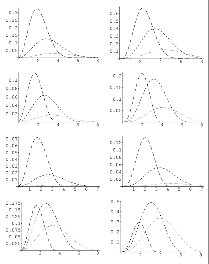
In Fig.6, as the caption suggests, we have placed the salient features of the integrands required to compute the total particle number density and the total energy density in the four different situations (universe without extra dimension, with static extra dimension, and with a dynamic extra dimension of two different kinds). We use the same value of the parameters (determining the minimum size of the ordinary scale factor) and (the slowness parameter) and the same values (which are the first three non-zero solutions found in Section III) in consecutive rows.
(a) The presence of a static extra dimension decreases the amplitudes for each mode, but the higher modes become relatively more dominating (i.e. relative contribution of higher modes w.r.t lower modes increases) in comparison with the case of a 4d universe.
(b) We have two different kinds of time-varying extra dimension (Fig.4). If the size of the extra dimension always remains less than the value equal to the static case and asymptotically reaches the same value (see ) in Fig.4), contributions of higher modes are significantly diminished and heights of the peaks are also decreased compared to the other cases. However, for the extra dimension with , an exactly opposite effect is seen to happen.
(c) In the last three rows, the -values where or peaks are the same and less than that in the 4d case.
(d) Previously, in models where the extra dimension was taken to be hidden and a decreasing function of time [7], any nonzero mode, if excited, was found to soon dominate over the redshifted -modes because of ever-increasing blueshift (their physical frequency asymptotically reaches a value equal to , but in the braneworld scenario can be much larger compared to those Planck-sized extra dimensions) resulting in a breakdown of the background cosmological model due to the possibility of a large back reaction. This problem may be resolved here for a dynamic extra dimension with , where the zero-mode is more dominant and higher mode contributions are quickly suppressed i.e production of [] particles can be controlled using suitable values of .
VII Non–thermal nature of the spectrum
In the cases of the massive, conformally coupled scalar field in four
dimensions and the analytic treatment of the time independent extra dimension
(assuming ) the spectrum of created particles can be
identified with that of a non–relativistic thermal gas of particles.
However, including the factor we find that the spectrum
deviates from the thermal nature–we might call it nearly thermal though.
The same features appear when we
consider time–dependent extra dimensions. In this section, we outline
these features by attempting to fit (by least-square fitting method) the
numerical data using thermal as well as non–thermal profiles characterised
by a set of parameters. The results are shown below.
In the case of a static extra dimension we attempt to fit total particle
number densities (top-left plot in right box of Fig.3)
with the following expressions for thermal and nonthermal profiles
of the particle number densities,
| (37) |
| (38) |
The first one is essentially the same thermal profile
as Eq.(35) with two new (fitting) parameters ( and )
introduced. The second one is a nonthermal profile with another parameter
() introduced to take care of the non-thermality. The best-fit plots are
shown in Fig.7 and Fig.8.
(a) Deviations of the datapoints from thermal fits are very prominent for
lower values of , whereas for higher and higher values of
data points seem to converge on the thermal fits. These features
are clearer when we use a non-thermal fit which seems to be a better fit
in all the three cases, but the extent of non-thermality decreases with
increasing (i.e., value of converges towards ), this is due to the fact that the factor contributes lesser and lesser for larger and larger .
(b) The fall–off of , for large k, are much faster than the thermal fits. Again this is confirmed through non-thermal fits where is found to be greater than .
(c) To figure out a single possible fitting formula for the non-thermal
profile with a unique set of parameters
one needs to do a rigorous statistical analysis.
The immediately apparent features of the parameters
in our fitting functions are the following. With increasing we
find: increasing, showing an oscillatory behaviour and
converging towards . These patterns can be useful in determining
the nature of non-thermality–an aspect which seems to be crucial
in distinguishing between the presence and absence of extra dimensions.


VIII The zero mode
In [7], it is pointed out that, in a radiative universe modes or the massless particles in the four dimensional picture will not be created if we have a static extra dimension because this situation is equivalent to the problem of massless particle creation in a conformally flat four dimensional cosmology. This accidental recovery of conformal invariance happens only because of the particular choice of (, in radiative universe) with a static extra dimension. Even in the case of a time-varying extra dimension conformal invariance can be imposed by making (the trivial case is, when , which is not of any interest). Otherwise, the conformal invariance is always broken for a metric of type Eq.(1) and the zero mode particles will indeed be produced with cosmological evolution. In Fig.9, features of zero mode particle creation in presence of a static extra dimension (continuous line) is compared with the other two situations with different kinds of extra dimensions (: smaller dashes and : longer dashes).

The contribution of zero mode particles, in the static case, lies between those of the two dynamic cases (this feature is similar for the other modes). For these particular choices of parameters, the zero modes are the most dominating modes. But the plots of the integrand in the total particle number density, asymptotically reaches a particular value as (for the zero modes), which is not the case for modes. Moreover, nothing similar to these modes (as the modes) exist in a four dimensional universe (without any extra dimension), since such a geometry is conformally flat.
IX Conclusions and comments
In this article, we have investigated the possible effects of the presence of a warped extra dimension (static or dynamic) on particle production in a 4d universe. From the numerical analysis represented via the figures, it is easy to point out the characteristic features.
The warp factor plays its part through the values of which are the allowed modes arising because of the warped extra dimension. will have discrete values in the case of a two brane model, otherwise it will be a continuum.
The location and heights of the peaks in the plots for the particle number density and energy density (as a function of ) decreases in the presence of an extra dimension. This is a feature of the breaking of conformal invariance and is manifest through the presence of the factor.
For the scenario with a time-varying extra dimension we have looked at two types distinguished through the parameter in the expression for . We note an increase in the heights of the peaks for and a decrease for ). To understand further general features of the breaking of conformal invariance in the context of particle creation one needs to see what happens for different kinds of models (i.e choices of and which yield different forms for ).
It may be mentioned that though these features look to be case specific and model dependent, it is worth noting that we did not choose arbitrarily. Rather, as mentioned before, it is chosen to be equal to (avoiding the introduction of another new parameter) or asymptotically reaching the same value (in the dynamic cases). Moreover, this value is the minimum value of during its evolution. In effect we are assuming some correlation between and , i.e. there may be a single mechanism which drives both the scale factors and therefore their ought to be a connection between them. This aspect can become clearer if we try to find out such solutions of the Einstein equations with a driving source in the bulk.
We have also found a mechanism (for ) to have control over contributions of higher non-zero modes to the energy density of the universe. We can suppress the production of those higher modes at our will by choosing higher and higher value of . The back reaction thus remains negligible and the classical cosmological model which is our background for all these studies does not break down.
To get an idea about the thermal/non–thermal nature of the spectrum of created particles we have tried to fit our numerical data with a thermal profile with a new set of parameters. Our analysis reveals that the spectrum could be assumed to be nearly thermal though marked deviations seem to appear for larger values of .
As a next step, one should study particle creation in the context of more realistic cosmological models and also further investigate the possibility of creation of other types of particles (like fermions, or spin one particles etc.) on the brane. Also, studies on particle production along the brane could provide insights into the recently proposed idea of braneworld isotropisation [20].
We admit, in conclusion, that our results are based on a toy scenario and can only be thought of as a build-up towards the study of more relevant and realistic situations in future. However, we do believe that some of the features observed (eg. possible avoidance of significant back–reaction effects and non-thermal nature of the spectral profile) here will indeed be carried over in generically similar situations and can provide pointers towards a better understanding of quantum fields in the presence of a warped extra dimension.
Acknowledgements
The authors thank G. Niz, A. Padilla and F. Urban for making them aware of related works and also for their useful comments. SG thanks IIT Kharagpur, India for providing financial support and the Centre for Theoretical Studies, IIT Kharagpur, India for allowing him to use its research facilities.
References
- [1] Th. Kaluza, Sitzunober. Preuss. Akad. Wiss. Berlin, p.966 (1921); O. Klein, Z. Phys. 37 895 (1926).
- [2] G. Gogberashvili, Int. J. of Mod. Phys. D 11, 1635(2002).
- [3] L. Randall and R. Sundrum, Phys. Rev. lett. 83 3370 (1999).
- [4] L. Randall and R. Sundrum, Phys. Rev. lett. 83 4690 (1999).
- [5] N. Arkani-Hamed, et al. Phys. Rev. lett. 84 586 (2000).
- [6] B. Bajc and G. Gabadadze, Phys. Lett. B 474, 282 (2000); S. Randjbar-Daemi and M. Shaposhnikov, Phys. Lett. B 492, 361 (2000); S. L. Dubovsky, V. A. Rubakov and P. G. Tinyakov, Phys. Rev. D 62, 105011 (2000); Y. Grossman and N. Neubert, Phys. Lett. B 474 361 (2000); C. Ringeval, P. Peter, J. P. Uzan, Phys. Rev. D 65, 044416 (2002); S. Ichinose, Phys. Rev. D 66, 104015 (2002); R. Koley and S. Kar, Class. Quantum Grav. 22, 753 (2005);
- [7] J. Garriga and E. Verdaguer, Phys. Rev. D 39 1072 (1989).
- [8] S. Nojiri and S. D. Odintsov, JCAP 06 004 (2003).
- [9] M. K. Mak and T. Harko, Class. Quantum Grav. 16 4085 (1999).
- [10] W. H. Huang, Phys. Lett. A140 280 (1989).
- [11] A. A. Saharian Phys. Rev. D 73 44012 (2006).
- [12] C. Bambi and F. R. Urban, Phys. Rev. Lett. 99 191302 (2007).
- [13] N. D. Birrell and P. C. W. Davies, Quantum fields in curved space (Cambridge University press, Cambridge, 1982) and references therein.
- [14] Ya. B. Zel’dovich and A. A. Starobinsky, Zh. Eksp. Teor. Fiz. 61, 617, (1981) [Sov. Phys. JETP 34, 1159 (1972)].
- [15] J. Audretch and G. Schäfer, Phys. Lett. A 66 459 (1978).
- [16] P. Binetruy, C. Deffayet, D. Langlois, Nucl.Phys. B565 269 (2000); P. Binetruy, C. Deffayet, U. Ellwanger, D. Langlois, Phys.Lett. B477 285 (2000); N. Kaloper, Phys.Rev. D60 123506 (1999); P. Bowcock, C. Charmousis, R. Gregory, Class.Quant.Grav. 17, 4745 (2000); P. Brax and C. van de Bruck, Class.Quant.Grav. 20 R201 (2003)
- [17] Je-An Gu, W-Y. P. Hwang, Phys.Rev. D66 024003 (2002), K. Freese and M.Lewis, Phys. Letts. B540, 1 (2002); J. Cline and J. Vinet, Phys. Rev. D68 025015 (2003)
- [18] D. J. H. Chung and K. Freese, Phys.Rev. D 61 023511 (2000); A. Wong, R-G Cai and N. O. Santos, Nucl.Phys. B797, 395 (2008).
- [19] T. Appelquist, A. Chodos and P. G. O. Freund, Modern Kaluza–Klein theories (Addison Wesley Publishing Company, 1987)
- [20] G. Niz, A. Padilla and H. K. Kunduri, arXiv:0801.3462