LPT–Orsay 08/38
FTUAM 08/6
IFT-UAM/CSIC-08-21
IFT-6/2008
Determining the WIMP mass using the complementarity between direct and indirect searches and the ILC
N. Bernal1, A. Goudelis1,Y. Mambrini2, C. Muñoz3,4
1 Laboratoire de Physique Théorique, Université Paris-Sud, F-91405 Orsay, France
2 Institute of Theoretical Physics, Warsaw University, ul. Hoza 69, 00-681 Warsaw, Poland
3 Departamento de Física Teórica C-XI, Universidad Autónoma de Madrid,
Cantoblanco, 28049 Madrid, Spain
4 Instituto de Física Teórica UAM/CSIC, Universidad Autónoma de Madrid,
Cantoblanco, 28049 Madrid, Spain
Abstract
We study the possibility of identifying dark matter properties from XENON–like kg experiments and the GLAST satellite mission. We show that whereas direct detection experiments will probe efficiently light WIMPs, given a positive detection (at the 10% level for GeV), GLAST will be able to confirm and even increase the precision in the case of a NFW profile, for a WIMP-nucleon cross-section pb. We also predict the production rate of a WIMP in the next generation of colliders (ILC), and compare their sensitivity to the WIMP mass with the XENON and GLAST projects.
1 Introduction
There exists strong evidence that a large fraction of the matter in our Universe is non-luminous [1]. Such evidence includes the motion of cluster member galaxies [2], gravitational lensing [3], cosmic microwave background [4], observations of the flat rotation curves of galaxies [5], etc. Dark matter plays a central role in current structure formation theories, and its microscopic properties have significant impact on the spatial distribution of mass, galaxies and clusters. Unraveling the nature of dark matter is therefore of critical importance. A Weakly Interacting Massive Particle (WIMP), with mass lying from the GeV to the TeV scale, is one of the preferred candidates for the dark matter of the Universe.
Different experimental programs are developing huge efforts to observe and identify the particle nature of dark matter. This can be achieved by direct measurement of the recoil energy of a nucleus when scattered by a WIMP, or indirectly via the observation of WIMP annihilation products. In both cases, the sensitivity depends strongly on the background and on the theoretical assumptions of the model. It would be interesting to combine all these efforts to invent intelligent strategies for determining the nature of dark matter [6]. Recently, several works (see, for example, Refs. [7] and [8] for the case of direct detection and [9, 10] for the indirect detection case) have shown that precision measurements of the mass of WIMPs are not only reserved to the domain of accelerator physics. In all of these studies, model independent bounds are derived for annihilation cross-sections, masses or WIMP–nucleus scattering cross-sections. The drawback of a model-independent framework (lack of determined microscopic processes) is largely compensated by the universality of the method: instead of restricting a theoretical parameter space, we restrict observable physical quantities (masses, branching ratios). Indeed, these limits are valid for a great number of WIMP candidates such as, for example, the supersymmetric neutralino, the lightest Kaluza Klein excitation, etc.
The aim of the present work is to analyse two of the most promising experiments, XENON [11] and GLAST [12], calculating and comparing their sensitivity to a WIMP mass depending on the astrophysical hypothesis (velocity distribution of WIMPs, density profile of the galactic halo). In addition, using the known cosmological abundance of dark matter in the Universe, we estimate the radiative WIMP production rate in the next generation of colliders (ILC) and compare their sensitivity to the WIMP mass with the XENON and GLAST projects.
Our goal is not to perform an exhaustive analysis of the mass determination capacity of each detection mode. The GLAST discovery potential has been studied in much detail in ref.[9] whereas direct detection experiments are thoroughly treated in refs. [7] and [8]. Instead, we are mostly interested in examining at which point and under which circumstances the different detection techniques can achieve comparable precision, thus acting in a complementary way (an issue which has been commented upon in a great number of references but has never been treated as such). In the case of indirect detection, we will restrict ourself to WIMP annihilation final states. It is well known, and is demonstrated in the Appendix, that different Standard Model particles contribute differently in the gamma-ray spectrum, the most prominent example being leptonic final states which tend to produce harder gamma-ray spectrae. Nevertheless, we should say in advance that at least in the ILC section we include an electron-positron final state, whereas the spectrum can be considered quite representative of bosonic and hadronic ones.
The paper is organised as follows. In section 2 we discuss the event rate and WIMP-nucleon scattering cross-section for a XENON-like experiment, in a microscopically model-independent approach. In Section 3 we carry out a similar analysis for the GLAST experiment, discussing in this case the WIMP annihilation cross section, and taking into account different halo profiles. Section 4 is dedicated to the comparison between these two modes of detection. In Section 5 we analyse the sensitivity that we can expect in such a model-independent framework for a linear collider. Finally, in Section 6 we carry out the comparison between the three detection modes. The conclusions are left for Section 7.
2 Direct detection
2.1 Differential event rate
In spite of the experimental challenges, a number of efforts worldwide are actively pursuing to directly detect WIMPs with a variety of targets and approaches. Many direct dark matter detection experiments are now either operating or in preparation. All these experiments measure the number of elastic collisions between WIMPs and target nuclei in a detector, per unit detector mass and per unit of time, as a function of the nuclear recoil energy . The detection rate in a detector depends on the density GeV cm-3 and velocity distribution of WIMPs near the Earth. In general, the differential event rate per unit detector mass and per unit of time can be written as:
| (2.1) |
where the WIMP-nucleus cross section, , is related to the WIMP-nucleon cross section, , by , with the WIMP-nucleon reduced mass, the WIMP-nucleus reduced mass, the WIMP mass, the nucleus mass, and the atomic weight. is the form factor.
For the velocity distribution we take a simple Maxwellian halo
| (2.2) |
where km/s is the velocity of the Sun around the galactic center with its uncertainty, and we have neglected the motion of the Earth around the Sun. After integrating over the angular part in order to find the speed distribution we get:
| (2.3) |
The integration over velocities is limited to those which can give place to a recoil energy , thus there is a minimal velocity given by .

The effective interaction between the WIMP and a nucleus is given by the Woods-Saxon form factor
| (2.4) |
where the transferred momentum is , is a spherical, first-order Bessel function, with fm, is the mass number, and fm.
In Fig.1 we show an example of a signal with a standard neutron background in a XENON–like ( kg) experiment, after years of data acquisition, as a function of the recoil energy. For a WIMP mass of GeV and a WIMP–nucleon cross-section of pb, such an experiment would reach a pretty large per degree of freedom () , of the order of 60.
2.2 The statistical method
In order to plot discrimination capacity regions, we use a method inspired by the treatment presented in [7]. For a WIMP with mass and a WIMP-proton scattering cross-section (in the case of indirect detection will, of course, be replaced by the total thermally averaged annihilation cross-section ), we can calculate the theoretically expected number of events, say , simply by integrating Eq.(2.1) from , the threshold energy which we consider as keV, up to , the maximal observable energy, which we take as equal to keV. Now, in a real-life experiment, one would expect the observed number of events to slightly deviate from this ideal value giving, say, events. In order to approach a more realistic situation, we perform our estimations not starting from , but rather from , where the “experimental” number of events is drawn from a Poisson distribution with mean value . Then, we can Monte-Carlo generate events according to Eq.(2.1) and we obtain what could actually resemble to an experimental spectrum. Such a set of events, together with the corresponding value of will be in the following referred to as an “experiment”.
Then, for every point in the parameter space , we calculate the corresponding extended likelihood function which is given by:
| (2.5) |
where
| (2.6) |
is the normalized total event rate (signal+background) and is the theoretical number of events, expected from Eq.(2.1), for the given point of the parameter space. The normalization renders a probability density function and, thus, suitable for use in a likelihood calculation.
The use of equation (2.5) presents the advantage that it takes into account the fact that the number of observed events in an experiment can, actually, deviate from the expected behaviour for several reasons. For the given experiment, say , we scan over the parameter space and calculate the value that maximize the expression (2.5). This is the estimation for the -th experiment. We then calculate the mean value of all the estimations and find which experiment’s estimation was closest to this mean value. This experiment is considered to be the most representative of them all and is used to perform a final scan. Finally, from the likelihood distribution we obtain through this scan we can plot discrimination capacity regions.
Direct Detection experiments present the advantage of quite well-controlled background. The additional ambiguity that arises in Indirect Detection and concerns uncertainties in the background will be dealt with in the relevant chapter.
As a final remark on the statistical treatment we used, let us say that in order to be more precise, we would have to take into account (as is systematically done in [9]) the fact that the mass and cross-section precision are themselves random variables and should, consequently, be given with their relevant statistical variance. To do so, we would have to consider the actual distribution of estimators for all experiments. However, as discussed in the Introduction, such a treatment goes far beyond the scopes of this paper, where we are interested in a more qualitative comparison of different detection modes. In this respect, we keep the experiment which averages the properties of a larger set of experiments. Motivating this approach, our results are indeed in accordance with [9] and [8].
2.3 The XENON experiment
The XENON experiment at the Gran Sasso national laboratory aims at the direct detection of dark matter via its elastic scattering off xenon nuclei. It was deployed underground in March and has been in continuous operation for a period of about one year. It allows the simultaneous measurement of direct scintillation in the liquid and of ionization, via proportional scintillation in the gas. In this way, XENON discriminates signal from background for a nuclear recoil energy as small as keV. Currently a kg detector is being used, but the final mass will be ton of liquid xenon. In Fig.2, we show the sensitivity curve for Xenon10 ( kg) and Xenon1T ( ton) for years of data acquisition, supposing zero backgrounds and a perfectly known velocity of the sun around the galactic center, fixed at km/sec.
In our study, following Ref. [11] we will consider the energy range between and keV and years of data acquisition for a kg XENON experiment. Such experimental conditions and time of exposure can be achieved after the years of GLAST mission and justify the comparison between the two detection modes.


In Fig.3 we show the ability of XENON to determine the mass and scattering cross-section for a , and GeV WIMP. We can clearly see how sensitive the experiment is to light WIMPs: the precision can easily reach the percent level for 11 1 During the finalization of this work, Drees and Shan in Ref. [7] proposed that one can even increase such a precision with a combined analysis of two experiments of direct detection. GeV. Indeed, the recoil energy of the nucleus depends on the reduced mass (see Eq.(2.1)). For WIMPs much heavier than the nucleus mass ( GeV for Xenon), , and is therefore independent of the WIMP mass. This is clearly reflected in the uncertainties at and CL in Fig.3 for a 500 GeV WIMP.
2.4 Influence of astrophysical/background assumptions
As mentioned before, a significant uncertainty (of the order of %) exists for the largely used values of the sun’s circular velocity around the Galactic Center (GC), as well as the various background forms we could expect in direct detection experiments. In this respect, it would be interesting to examine how the previous results are altered in the case where is actually included in the fitting procedure, letting it vary within the given margin of error.
As far as background events are concerned, it is quite difficult to perform a general study valid for every detector. Neutron backgrounds, which are in fact the most difficult to distinguish from signal events, are usually taken to come from three sources (see also [13]):
- •
Cosmic muon - induced neutrons, which are not in general considered to cause much nuisance.
- •
Neutrons from the detector’s surrounding rock.
- •
Neutrons coming from contamination of the detector itself or surrounding
materials.
As we said, it is difficult to model in general neutron backgrounds, as they are mostly determined by the specific location in which every experiment is situated, as well as by the specific shielding configuration adopted by each collaboration. Two widely studied forms of neutron backgrounds are the case of a constant one, which seems to be quite well-motivated by an experimental point of view and can resemble to a heavy WIMP’s signal, and an exponential one which apart from its theoretical motivation is also interesting as it gets to “mimic” (as pointed out in [8]) the actual signal spectrum for intermediate WIMP masses. In this respect, we studied the impact of these two forms of background:
We consider firstly a constant background, with a value taken to be the same as the maximal WIMP signal in the first energy bin. Throughout this paper, when examining the impact of uncertainties on the mass determination accuracy, we will consider the case of a somehow “typical” in many theoretical frameworks case of a 100 GeV WIMP.
Then, we introduce an exponential background of the form , where the slope of the exponential is fixed at keV and the factor is determined by demanding that the maximal values of the signal and the background be the same. The reason for this specific choice of parameters is that it is for these values that the signal spectrum has a significant resemblance to the background one, making it difficult to distinguish from one another.


Our results are shown in Figs.4 and 5 for the cases of inclusion of in the fitting procedure and non-zero backgrounds respectively. The deterioration of the expected accuracy is obvious, when we compare these plots to those of Fig.3. Especially for the case of large uncertainties in (we let it vary in the whole margin-of-error region) and of inclusion of a background which is nearly degenerate with the signal, the expected precision is dramatically aggravated. This shows, among others, the extreme importance of a well-controlled environment and well-measured input parameters, other than the WIMP mass.
3 Indirect detection
3.1 Differential event rate
The spectrum of gamma–rays generated in dark matter annihilations and coming from a direction forming an angle with respect to the galactic center is
| (3.7) |
where the discrete sum is over all dark matter annihilation channels, is the differential gamma–ray yield, is the annihilation cross-section averaged over its velocity distribution, is the branching ratio of annihilation into final state “i” , and is the dark matter density. The method followed in order to obtain the spectral function describing the standard model particle decay into -rays, is presented in the Appendix.
| (kpc) | |||||
|---|---|---|---|---|---|
| NFW | |||||
| Moore et al. | |||||
It is customary to rewrite Eq. (3.7) introducing the dimensionless quantity (which depends only on the dark matter distribution):
| (3.8) |
After having averaged over a solid angle, , the gamma–ray flux can now be expressed as
| (3.9) | |||||
The value of depends crucially on the dark matter distribution. The most common parametrization of the different profiles that have been proposed in the literature is
| (3.10) |
where is the local (solar neighborhood) halo density, is a characteristic length, and the distance from the Sun to the galactic center. As mentioned above, we will use GeV/cm3 throughout the paper, but since this is just a scaling factor in the analysis, modifications to its value can be straightforwardly taken into account in the results. N–body simulations suggest a cuspy inner region of dark matter halo with a distribution where generally lies in the range (NFW profile [14]) to (Moore et al. profile [15]), producing a profile with a behavior at small distances. Over a solid angle of sr, such profiles can lead from to . Moreover, if we take into account the baryon distribution in the Galaxy, we can predict even more cuspy profiles with in the range to () through the adiabatic compression process (see the study of Refs. [16, 17]). We summarize the parameters used in our study and the values of for each profile in Table 1. The values contained in the Table were calculated using the darkSUSY package for calculations of fluxes coming from SUSY DM candidates’ annihilations. The calculation is obviously not altered whatever DM candidate is assumed and is therefore valid for an arbitrary WIMP as the ones examined here.
It is worth noticing here that we are neglecting the effect of clumpyness, even though other studies showed that, depending upon assumptions on the clumps’ distribution, in principle an enhancement of the flux by a factor of to is possible [18]. In this respect, the following predictions on the gamma-ray flux from the galactic center are conservative.
3.2 Modeling the galactic center background.
HESS [19] has measured the gamma–ray spectrum from the galactic center in the range of energy [ GeV– TeV]. The collaboration claims that the data are fitted by a power–law
| (3.11) |
with a spectral index and . The data were taken during the second phase of measurements (July–August, ) with a of per degree of freedom. Because of the constant slope power–law observed by HESS, it turns out possible but difficult to conciliate such a spectrum with a signal from dark matter annihilation [17, 20]. Indeed, final particles (quarks, leptons or gauge bosons) produced through annihilations give rise to a spectrum with a continuously changing slope. Several astrophysical models have been proposed in order to match the HESS data [21]. In the present study we consider the astrophysical background for gamma–ray detection as the one extrapolated from the HESS data with a continuous power–law over the energy range of interest ( – GeV). As was recently underlined in Ref. [22], the sensitivity of GLAST will be affected by the presence of such an astrophysical source. Note that the WIMP masses that we shall obtain in our parameter space TeV avoid any conflict with the observations of HESS.
In addition, we have also taken into account the EGRET data [23] in our background at energies below GeV (), as they can affect the sensitivity of the analysis. Indeed, the extrapolation of the gamma–ray fluxes measured by HESS down to energies as low as GeV is likely to be an underestimation of the gamma–ray background in the galactic center, as EGRET measurements are one to two orders of magnitude higher than the HESS extrapolation. The EGRET point-source has been found [10] to be well fitted by a simple power-law with slope . We thus decided to take as background an interpolation between the HESS extrapolation and the EGRET data below GeV to stay as conservative as possible in evaluating the gamma–ray background.
Finally, we will consider the diffuse background of gamma rays in the region surrounding the galactic center.
We will describe the spectrum of the background using the HESS observation from the Galactic Center Ridge [19], which can be described by
| (3.12) |
In our analysis, we will consider the inner field of view ( sr) and the energy region between and GeV. During the completion of our work, the authors of Ref. [10] gave a more detailed and sophisticated statistical analysis of the diffuse background, adopting an overall normalization around the galactic center and taking into account a statistical spread function as GLAST would be able to probe in this region. However, we have checked that our results are not significantly modified and we recover similar results concerning the prospects of GLAST.
3.3 The GLAST experiment
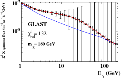
The space–based gamma–ray telescope GLAST [12] was launched in May for a five-year mission. It will perform an all-sky survey covering a large energy range ( – GeV). With an effective area and angular resolution of the order of and ( sr) respectively, GLAST will be able to point and analyze the inner center of the Milky Way ( pc). Concerning the statistical method, we have used an analysis similar to the one considered in the case of direct detection in section 2.2, with a six-year mission run, assuming the galactic center will be within its field–of–view of the time [12, 26]. In Fig.6 we show the ability of GLAST to identify a signal from dark matter annihilation for a WIMP mass of GeV. The error bars shown are projected assuming Gaussian statistic, and we adopt the background described above including Poisson noise. In the following, we will concentrate on a process which gives annihilation to . We have checked that the dependence on the final state does not influence significantly the general results of the study, except in the case of leptonic final states. This will be studied in a specific case in Section 5 dedicated to the ILC experiment.

In Fig.7 we show the ability of GLAST to determine the mass and annihilation cross-section for a , and GeV WIMP. Again, we can see that the experiment is more sensitive to light WIMPs: the precision can easily reach the percent level for GLAST for GeV. The gamma–ray spectrum will give more precise measurements if the mass of the WIMP lies within the GLAST sensitivity range. Indeed, the shape of the spectrum will be easily reconstructed above the HESS/EGRET and diffuse background if the endpoint of the annihilation spectrum lies within the energy range reachable by GLAST [ GeV]. Furthermore, we have studied the influence of the variation of the inner slope of the halo profile on the resolution of the WIMP mass. In addition to the NFW profile, we have considered some NFW–like profiles, allowing the parameter in Eq.(3.10) to vary from its original value by . This is shown in Fig.8, where in addition to the NFW halo profile () we also study profiles with . As expected, the larger the is, the more enhanced the galactic gamma ray flux becomes, and the better the WIMP mass resolution turns out to be. It is worth noticing here that in the case of a compressed NFW profile (), the precision of GLAST increases by two orders of magnitude.

3.4 Varying background parameters
Throughout the previous (and the following) analysis, we have considered a perfectly known background for both detection modes. Whereas this is a rather reasonable approximation for the case of direct detection, it is less obvious for the indirect one. As it has been pointed out (see, for example, [24, 25]), the uncertainties entering the calculation of the backgrounds coming from the galactic center region can considerably affect the results of any analysis. More concretely, and especially for small WIMP masses and low energies (where the performance of both direct and indirect detection is maximal), the main contribution in background comes from the EGRET source aforementioned. However, both the overall normalisation and the spectral index characterising this source’s spectrum contain uncertainties, and it has been widely discussed in the literature that a dark matter annihilation signal could account for some part of the EGRET source signal. An interesting point would be to include the overall background normalization as well as the spectral index in the fitting procedure. In Fig.9 we show, for the sake of comparison, the result of a fitting procedure, where we also fit the background normalization while simultaneously considering signals and backgrounds with poissonian fluctuations. The original spectrum is taken to be the full EGRET source plus the flux produced by a GeV WIMP annihilating in a NFW halo. One could imagine discarding low-energy data which contain a maximal background contamination. This, however, would significantly reduce the statistics and the corresponding precision, since a major part of the signal would be discarded. The fact that the inclusion of an uncertainty in the background normalization (i.e. its inclusion in the statistical treatment) does not have a major impact on the results can be explained from the fact that throughout this work we have used eq.(2.5) in our statistical analysis, which already introduces a deviation from the ideally expected situation. In this respect, our results are quite conservative.
In the same way, in Fig.10 we show the corresponding results where this time the spectral index is included in the fitting procedure instead. The spectral index is left to vary in the region , which we find to be a quite reasonable one as we verified that all over this region we obtain reasonable fits of the EGRET data.


It is interesting to note that the variation of the background’s spectral index seems to have a larger impact on the precision that could be achieved, with respect to the corresponding case of the background’s overall normalisation.
This is somehow logical, first of all since by definition the background depends linearly on the normalisation factor, but exponentially on the spectral index of the EGRET point source. So, modifications in the latter bring along a much more drastic modification of the background signal itsself. Furthermore, variations of the overall normalisation have just the influence of "burying" the signal a little more or a little less in a background which is already quite elevated. On the contrary, by varying the spectral index we actually change the shape of the spectrum. This brings along a more important uncertainty, since we could imagine much more numerous configurations in the (spectral index, cross-section, mass) space that could satisfy selection criteria.
3.5 Impact of Final States
Again, throughout this paper, we have considered a pure WIMP annihilation into a final state. This is an assumption which is made to simplify the overall treatment, but which at the same time somehow restricts the generality of our results. In this paragraph, we are interested in examining what could be the impact of variations in the final state on the WIMP mass determination capacity. Annihlation into pairs is not expected to seriously modify the results, what would be more interesting would be to see what happens when we consider (light or heavy) quark pairs and/or leptons as WIMP annihilation products.
The spectrae of SM particles’ annihilations into gamma-rays can be found in the Appendix. As explained there, the only leptonic final state we consider is the one, since annihilation into has a relatively small contribution to the annihilation gamma-ray spectrum, whereas pairs contribute through other processes, the examination of which exceeds the purposes of the present treatment. We should, nevertheless, note here that we do not take into account the effects of leptonic final state radiation which can indeed become important, especially in the case of Kaluza-Klein dark matter and in energy ranges lying near the WIMP mass. The effect of such processes has been discussed in detail in refs.[27] for the case of a generic WIMP and [28] for the special case of KK dark matter. Obviously, this omission somehow retricts the generality of our results as far as the impact of final states are concerned.
To this goal, we performed two kinds of tests: The first one consists only of modifying the annihilation products, considering a perfectly known final state (meaning that the Branching Ratios are not included in the statistical treatment). Our results can be seen in Fig.11 for the case of pure , and final states and a GeV WIMP.

It is interesting to notice the relative amelioration of the mass resolution with respect to the pure final state. A possible explanation could be that, as can clearly be seen in gamma-ray yields presented in the Appendix, fermionic final states tend to give more hard spectrae with respect to bosonic ones (the extreme case being leptonic ones), rendering the spectrum more easily distinguishable from the background. The hardest spectrum is given by the final state. Nevertheless, in this case the characteristic spectral form is somewhat compensated from the reduced statistics of the signal. This is not the case for annihilation into quarks, where the characteristic spectral form, although less obvious than in the leptonic case, is nevertheless combined with an important enhancement in the signal.
As a second test, we consider a mixed final state and fit the BRs themselves along with the annihilation cross-section and the WIMP mass. Our results can be seen in Fig.12 where we have taken a 100 GeV WIMP annihilating into a final state consisting of and . The sum of the two branching fractions is obviously equal to , so we only need to include one further parameter in the statistical analysis.

In this case, we can clearly see that the mass resolution deteriorates with respect to the case where a perfectly known final state is considered. A possible explanation could be that a mixed lepton - gauge boson final state yields a spectrum which presents neither the augmented statistics of pure annihilation into gauge bosons (the gamma-ray yield of leptons is significantly inferior to the one of gauge bosons) nor the characteristic hard spectral form of annihilation into pairs.
4 Direct versus indirect detection experiments
It is interesting to remark from Figs.3 and 7, how two completely different means of observation, with completely different signal/background physics, are in fact competitive (and hence complementary) in the search for the dark matter.
In Fig.13 we compare the precision level for both experiments as a function of the WIMP mass, for different values of the spin-independent cross-section (, and pb) and for different halo profiles. For this treatment we minimize the impact of uncertainties discussed in the previous paragraph, as we are mostly interested in examining the a priori, in some sense “intrinsic” sensitivity of the two detection techniques. For example, in the case of direct detection, the necessity for minimisation of background noises and control of the noise sources has been repeatedly stressed out. As for uncertainties entering the velocity distribution of WIMPs in the solar neighbourhood (or, why not, the form factor’s functional form), these can, in principle be minimized by measurements exterior to the experiments themselves. The same holds for uncertainties in the case of indirect detection. As a small example, Fermi-GLAST’s overall sky survey capacity is hoped to contribute in the minimisation of uncertainties in non-DM annihilation sources, whereas other observations in different energy regions can also contribute in this direction. In this respect, for our comparative results, we remove the extra parameters from the statistical treatment. We see that at of confidence level GLAST, after years of exposure ( years of taking data at of time exposure), will have an equivalent sensitivity to a kg XENON-like experiment after years of running if pb, independently of the WIMP mass. The indirect detection by GLAST will always be able to give an upper bound on the WIMP mass for GeV, whereas a XENON-like kg experiment would only give a lower bound value if pb. In all cases, the lower bounds given by GLAST for a NFW halo profile are similar to the ones given by a XENON-like kg experiment for any WIMP mass if pb.
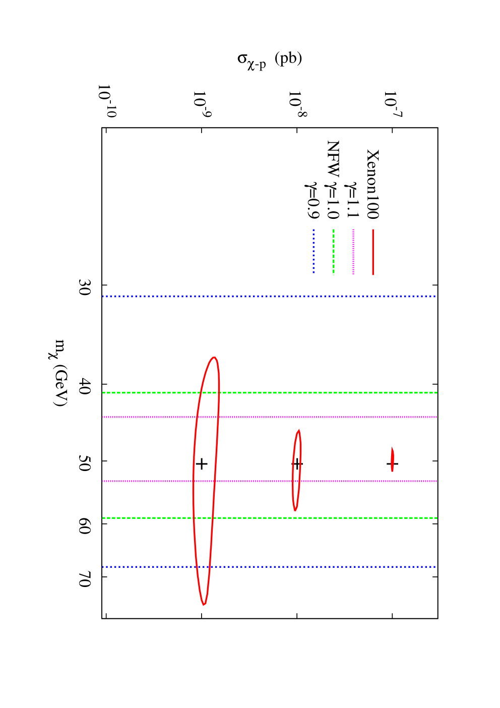
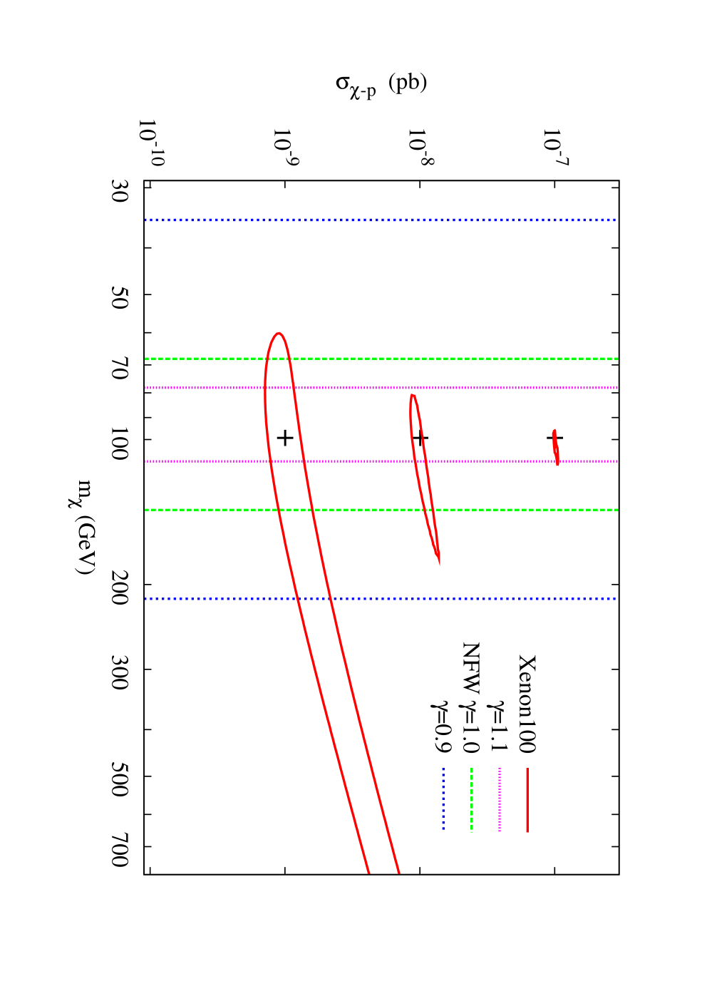
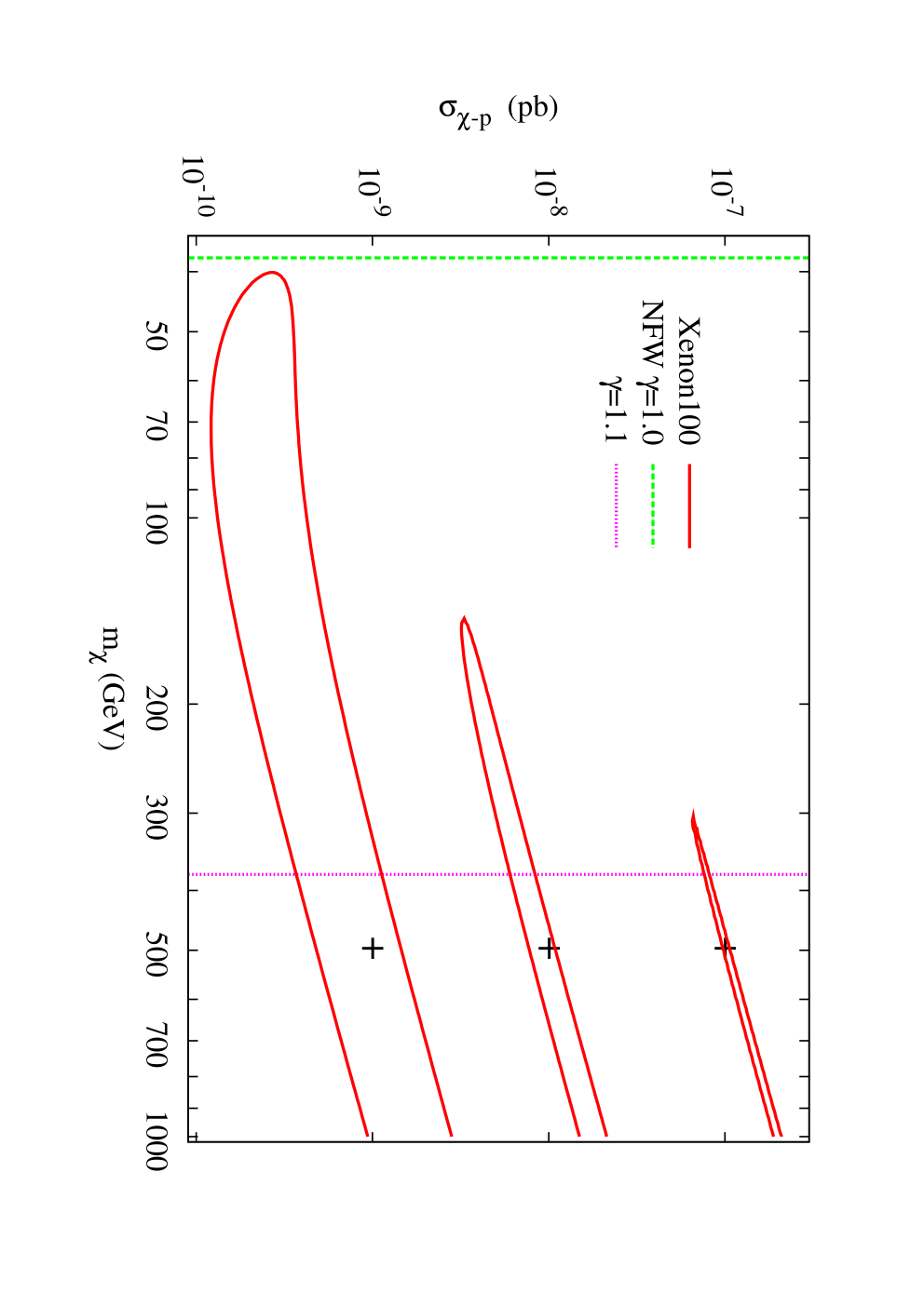
To compare the uncertainties on the WIMP mass expected from direct and indirect detection modes, we plotted in Fig.14 as a function of the WIMP mass for and a NFW halo profile. One can clearly see in the figure that GLAST will be competitive with XENON kg to measure the WIMP mass in the case of a NFW halo profile for pb.


5 WIMPs at present and future colliders
Among the most important sources of information concerning WIMP dark matter are, obviously, collider experiments, both present, such as the Tevatron or the Large Hadron Collider (LHC) and future, such as the International Linear Collider (ILC). In fact, there is a quite general agreement on the fact that despite the significant progress in astroparticle physics experiments, which manage to impose more and more constraints on various models, collider experiments remain an irreplaceable source of information for particle physics. It is quite natural thus, to examine the potential of colliders to constrain WIMP properties. We will examine the extent at which astroparticle and collider experiments become competitive, trying at the same time to stay as model-independent as possible.
This last point is, in fact, the major difficulty in treating collider experiments to extract astroparticle data: most studies performed for new physics at colliders are very strongly model dependent. This is almost unavoidable for the case of the LHC, due to the hadronic nature of the colliding particles. The large uncertainties on the parton distribution functions (and, hence, on the initial energy of the colliding particles/partons) render it extremely difficult (in fact, practically impossible) to look beyond the transverse plane. This fact obviously limits -up to a certain point- the precision that could be obtained with respect to, for example, an collider. As a result, it is quite difficult to make predictions in a model-independent way, since a whole set of parameters must be taken into account in order to perform concrete predictions. The cruciallity of these uncertainties will become clearer in the following.
5.1 The Approach
Recently, an approach was proposed in references [29, 30] which allows to actually perform a model-independent study of WIMP properties at lepton colliders (such as the ILC project). The goal we pursue is to extract constraints which are as stringent as possible for a generic dark matter candidate. A generic WIMP can annihilate into pairs of standard model particles:
| (5.13) |
However, the procedure taking place in a collider is the opposite one, having only one species of particles in the initial state. The idea proposed in Ref. [29] is to correlate the two processes in some way. This can be done through the so-called “detailed balancing” equation, which reads:
| (5.14) |
where and are respectively the velocity and the spin of the particle . The cross-section is only averaged over spins.
The total thermally averaged WIMP annihilation cross-section can be expanded as
| (5.15) |
where is the angular momentum of each annihilation wave. Now, for low velocities, the lowest-order non-vanishing term in the last equation will be dominant. So, we can express the total annihilation cross-section as a sum of the partial ones over all possible final states for the dominant partial wave in each final state:
| (5.16) |
Next, we can define the “annihilation fraction” into the standard model particle pair :
| (5.17) |
By combining Eqs. (5.14) and (5.17) we can obtain the following expression for the WIMP pair-production cross-section:
| (5.18) |
Now, a few remarks should be made about the validity of this formula:
- •
Equation (5.18) is valid for WIMP pair-production taking place at center-of-mass energies just above the pair-production threshold.
- •
The detailed balancing equation is valid if and only if the process under consideration is characterized by time-reversal and parity invariance. It is well known that weak interactions violate both of them, up to some degree, which we ignore in this treatment.
A process of the form is not visible in a collider, since WIMPs only manifest themselves as missing energy. At least one detectable particle is required for the event to pass the triggers. An additional photon from initial state radiation (ISR) is required to be recorded on tape: . We can correlate the WIMP pair-production process to the radiative WIMP pair-production for photons which are either soft or collinear with respect to the colliding beams. In this case, the two processes are related through [29]:
| (5.19) |
where , is the angle between the photon direction and the direction of the incoming electron beam, is the WIMP pair-production cross-section produced at the reduced center of mass energy , and is defined as:
| (5.20) |
The problem is that very collinear photons fall outside the reach of any detector, due to practical limitations in the coverage of the volume around the beam pipe. Also, typically, lower cuts are included in the detected transverse momentum of photons, , in order to avoid excessive background signals at low energies. So, if we are to use this approach, we have to examine its validity outside the soft/collinear region. The accuracy of the collinear approximation for hard photons at all angles has been discussed in the original paper [29], with the conclusion that the approach works quite well.
However, an important point should be taken into account here. From the previous discussion on the validity of the method, we have to impose specific kinematical cuts on the detected photons. We consider the following conditions:
- •
We demand an overall condition and GeV in order to assure the detectability of the photons.
- •
In order to assure the fact that any photon under examination corresponds to non-relativistic WIMPs, we demand . This gives a lower kinematical cut, along with an upper cut corresponding just to the endpoint of the photon spectrum:
(5.22)
These conditions present a flaw: the energy limits depend on the mass we wish to constrain. On the other hand, for the reasons explained before, we cannot treat the signals without imposing such kinds of cuts, if we do not want either to abuse the method or stick to heavy WIMPs (which, for kinematical reasons, cannot be relativistic). The only way to evade this problem is to suppose that other dark matter detection experiments (or, eventually, the LHC in the framework of specific models) will have already provided us with some sort of limits on the WIMP mass. In this case, having an idea of the region in which the WIMP mass falls, we can also estimate the cuts that will safely keep us outside the relativistic region and only consider photons within this region.
The main source of background events is the standard model radiative neutrino production, . Apart from these background events, various models predict additional signals of the form “ + missing energy”, one of the most well-known examples being radiative sneutrino production [31, 32], predicted in the framework of several supersymmetric models. In the spirit of staying as model-independent as possible, we will ignore all possible beyond standard model processes.
5.2 Basic Results
5.2.1 Non-polarized beams
We place ourselves in the framework of the ILC project with a center-of-mass energy of GeV and an integrated luminosity of fb-1. In order to estimate the background events, we used the CalcHEP code [33, 34] to generate events, corresponding to the aforementioned conditions. The total radiative neutrino production background can be seen in Fig.15. The peak at GeV corresponds to the radiative returns to the resonance.

We generate a predicted “observable” spectrum for given values of the WIMP mass and the annihilation fraction. During this study, we do not proceed to a (more realistic) full detector simulation, as done for example in Ref. [35], but stick to prediction levels in order to perform as thorough a scan as possible in the parameter space and to have a picture of the “a priori” potential of the method.


Figure 16 shows the predicted ability of the ILC to determine WIMP masses and annihilation fractions for four points in the parameter space for a and Confidence Level. These results concern WIMPs with spin and an angular momentum which corresponds to an annihilation cross-section pb [29]. As can be seen, we are able to constrain quite significantly the WIMP mass ( precision), while constraints on are weaker.
Figure 17 shows the relative error () for the mass reconstruction as a function of , for and a confidence level. The solid line corresponds to the proper treatment including kinematical cuts. For indicative reasons, we also show the abused results obtained if we do not impose kinematical cuts on the photon energy (dashed line). The amelioration of the method’s efficiency is obvious, although this is after all a false fact, since we include regions in which the approach is not valid. Above GeV the two lines become identical, since the WIMPs cannot be relativistic. The capacity of the method peaks significantly for masses of the order of GeV because around this value we reach an optimal combination of phase space volume and available spectrum that passes the kinematical cuts and can, hence, be used for the calculation of the relevant ; whereas as we move away from this value the accuracy tends to fall.
Let us make a final remark on the possibility of adopting a similar approach in the case of the LHC. As we argued before, the large uncertainties entering the parton distribution functions and, hence, the large uncertainty in the collision energy, affect significantly the precision of the whole procedure (which is, already, based on approximations). Formally, in order to perform such a study for the LHC, the computed cross-sections must be convoluted with the proton form factors. As an additional element, the photon background in the LHC is expected to be much greater than in the ILC. The possibility of determining WIMP properties through a model-independent method at the LHC has been addressed to in Ref. [36], where the authors conclude that WIMP detection will be extremely difficult, if even possible.
5.2.2 Polarized beams
The reach of the ILC can be further increased by polarizing the beams. For polarized beams, the signal cannot be fully characterized by ; instead, four independent annihilation fractions are needed, corresponding to the four possible helicity configurations.
To apply Eq. (5.21) to this case, we make the replacement:
| (5.23) | |||||
where are the polarizations of the positron and the electron beams. As in ref [29, 35], let us assume that the WIMP couplings to electrons conserve both helicity and parity: and .
In Fig.18 we show the relative error for the mass reconstruction for and confidence level, for the unpolarized scenario and for two different polarizations: and .

6 Complementarity
In Fig.19 we compare the precision levels for direct and indirect detection experiments, along with the corresponding results of the method we followed for the ILC for two cases of WIMPs masses, GeV and GeV, and . We plot the results in the plane. This is done as the parameter entering the ILC treatment presented before is, in fact, the same parameter as the corresponding branching ratio appearing in eq. (3.7) for .
| XENON | GLAST | ILC | |
|---|---|---|---|
| GeV | GeV | GeV | |
| GeV | GeV | GeV | GeV |
| GeV | GeV | GeV | GeV |
| GeV |
The blue-dotted line corresponds to a kg XENON-like experiment, where the WIMP-nucleus cross-section has been assumed to be pb. The green-dashed line depicts the results for a GLAST-like experiment assuming a NFW halo profile. The total annihilation cross-section into standard model particles has been taken to be cm3s-1. The red-plain line represents our results for an ILC-like collider, with non-polarized beams. All the results are plotted for a confidence level.
We can see that for different regions of the WIMP mass, the three kinds of experiments that we have used as prototypes can act in a highly complementary way. For example, for the case of a 100 GeV WIMP, indirect detection or an ILC-like experiment alone can provide us with limited precision both for the WIMP mass (of the order of ) and the parameter (where the results are even worse). Combined measurements can dramatically increase the precision, reaching an accuracy of in mass. If we additionally include direct detection measurement, we can further increase the precision.
For the case of a GeV WIMP, a point where the unpolarized ILC sensitivity peaks, we see that the dominant information comes from this source. Nevertheless, even if we only combine direct and indirect detection experiments, we see that we can, in fact, acquire non-negligible constraints on the dark matter candidate mass.
To summarize the analysis, we show in Table 2 the precision expected for several interesting dark matter masses. Whereas a light WIMP (50 GeV) can be reached by both types of dark matter experiments with a relatively high level of precision, our analysis fails in the ILC case because of the relativistic nature of the WIMP. On the contrary, the ILC would be particularly efficient to discover and measure a WIMP with a mass of about 175 GeV. Concerning a 500 GeV WIMP, which is kinematically unreachable at the linear collider, it would be difficult to be observed by GLAST or XENON. Only a lower bound could be determined experimentally.


7 Conclusions
A Weakly Interacting Massive Particle (WIMP), with mass lying from the GeV to the TeV scale, is one of the preferred candidates for the dark matter of the Universe.
We have discussed the possibility of identifying WIMP properties in a model-independent way. For that we have considered direct and indirect searches, and in particular the interesting cases of a XENON-like 100 kg experiment and the GLAST satellite. We have shown that whereas direct detection experiments will probe efficiently light WIMPs given a positive detection (at the level for GeV), GLAST will be able to confirm and even increase the precision in the case of NFW profile, for a WIMP-nucleon cross-section pb.
Moreover, both XENON and GLAST are complementary with a future ILC project, and the measurements from the three experiments will be able to increase significantly the precision that we can reach on the mass of the WIMP.
Acknowledgements
The authors want to thank particularly G. Bertone for the careful reading of the work. N.B. and A.G. would also like to thank R. K. Singh and A. Djouadi for useful discussions concerning the ILC part of the present work. Finally, A.G. would like to thank Y. Amhis for useful discussions concerning the statistical treatment.
Likewise, the authors would like to thank the ENTApP Network of the ILIAS project RII3-CT-2004-506222 and the French ANR project PHYS@COL&COS for financial support. Y.M. would like to thank the members of the Institute for Theoretical Physics of Warsaw for their warm hospitality, and financial support via the “Marie Curie Host Fellowship for Transfer of Knowledge”, MTKD-CT-2005-029466. The work of A.G. is sponsored by the hepTOOLS Research Training Network MRTN-CT-2006-035505. The work of C.M. was supported in part by the Spanish DGI of the MEC under Proyectos Nacionales FPA2006-01105 and FPA2006-05423, by the European Union under the RTN programs MRTN-CT-2004-503369 and UniverseNet MRTN-CT-2006-035863, and by the Comunidad de Madrid under Proyecto HEPHACOS S-0505/ESP-0346. The comments and suggestion of the referee were more than precious for the evolutions of the work.
Appendix
In this Appendix we present the method followed in order to obtain the functions describing the standard model particle decay into -rays. In order to determine these spectral functions, we generated 300000 events of standard model particles decaying (directly or through secondary decays) into -rays using the PYTHIA [37] package, taking care in order to include all possible decay channels. Following the method of Ref. [38], we fitted the resulting spectra through functions of the form:
| (7.24) |
where represents the i-th WIMP annihilation channel, ; with being the WIMP mass and are seventh-order polynomial functions which were found to be the following:
The case of WIMP annihilation into pairs has a relatively small decay contribution, to the photon spectrum, coming from the channel, which has a small branching ratio. pair production contributes to the gamma–ray spectrum through different (not decay) processes, mainly inverse Compton scattering and synchrotron radiation. These contributions depend crucially on the assumptions made concerning the intergalactic medium and will not be analysed here (For a relevant treatment see, e.g., section V of [39]). This means, practically, that the and spectral functions are set equal to zero. A graphical representation of these functions can be seen in Fig.20.
These functions can afterward be used in order to generate any gamma-ray flux according to eq. (3.7)


As we can see, all contributions are quite similar, apart from the channel which has a characteristic hard form. Nevertheless, at high energies, the form of all contributions becomes almost identical.
References
- [1] For reviews, see: G. Jungman, M. Kamionkowski and K. Griest, Phys. Rept. 267 (1996) 195; C. Munoz, Int. J. Mod. Phys. A 19 (2004) 3093 [arXiv:hep-ph/0309346]; G. Bertone, D. Hooper and J. Silk, Phys. Rept. 405 (2005) 279 [arXiv:hep-ph/0404175].
- [2] F. Zwicky, Helv. Phys. Acta 6, (1933) 110; S. Smith, Astrophys. J. 83 (1936) 23.
- [3] J. A. Tyso, G. P. Kochanski and I.P. Dell’Antonio, Astrophys. J. 498, L107 (1998); D. Clowe, M. Bradac, A. H. Gonzalez, M. Markevitch, S. W. Randall, C. Jones and D. Zaritsky, Astrophys. J. 648 (2006) L109 [arXiv:astro-ph/0608407].
- [4] D. N. Spergel et al. [WMAP Collaboration], Astrophys. J. Suppl. 170 (2007) 377 [arXiv:astro-ph/0603449]; E. Komatsu et al. [WMAP Collaboration], arXiv:0803.0547 [astro-ph].
- [5] A. Borriello and P. Salucci, Mon. Not. Roy. Astron. Soc. 323 (2001) 285 [arXiv:astro-ph/0001082].
- [6] D. Hooper and E. A. Baltz, arXiv:0802.0702 [hep-ph].
- [7] A. M. Green, JCAP 0708 (2007) 022 [arXiv:hep-ph/0703217]; C. L. Shan and M. Drees, arXiv:0710.4296 [hep-ph]; M. Drees and C. L. Shan, arXiv:0803.4477 [hep-ph].
- [8] A. M. Green, arXiv:0805.1704 [hep-ph].
- [9] Baltz, E. A. et al, JCAP 0807, 013 (2008) [arXiv:0806.2911];
- [10] D. Hooper and D. P. Serpico, JCAP 0706, 013 (2007) [arXiv:astro-ph/0702328]; M. Kachelriess and P. D. Serpico, Phys. Rev. D 76 (2007) 063516 [arXiv:0707.0209 [hep-ph]]; S. Dodelson, D. Hooper and P. D. Serpico, Phys. Rev. D 77 (2008) 063512 [arXiv:0711.4621 [astro-ph]].
- [11] J. Angle et al. [XENON Collaboration], arXiv:0706.0039 [astro-ph].
- [12] N. Gehrels and P. Michelson, Astropart. Phys. 11 (1999) 277.
- [13] Aprile, E. et al. [XENON Collaboration], [arXiv:astro-ph/0207670].
- [14] J. F. Navarro, C. S. Frenk and S. D. M. White, Astrophys. J. 462 (1996) 563 [arXiv:astro-ph/9508025]; J. F. Navarro, C. S. Frenk and S. D. M. White, Astrophys. J. 490 (1997) 493 [arXiv:astro-ph/9611107].
- [15] B. Moore, S. Ghigna, F. Governato, G. Lake, T. Quinn, J. Stadel and P. Tozzi, Astrophys. J. 524 (1999) L19.
- [16] F. Prada, A. Klypin, J. Flix, M. Martinez and E. Simonneau, arXiv:astro-ph/0401512; G. Bertone and D. Merritt, Mod. Phys. Lett. A20 (2005) 1021 [arXiv:astro-ph/0504422]; G. Bertone and D. Merritt, Phys. Rev. D72 (2005) 103502 [arXiv:astro-ph/0501555]; E. Athanassoula, F. S. Ling and E. Nezri, Phys. Rev. D72, 083503 (2005) [arXiv:astro-ph/0504631].
- [17] Y. Mambrini, C. Munoz, E. Nezri and F. Prada, JCAP 01 (2006) 010 [arXiv:hep-ph/0506204].
- [18] L. Bergstrom, J. Edsjo, P. Gondolo and P. Ullio, Phys. Rev. D 59 (1999) 043506 [astro-ph/9806072].
- [19] F. Aharonian et al. [HESS Collaboration], Astron. Astrophys. 425 (2004) L13 [arXiv:astro-ph/0408145].
- [20] S. Profumo, Phys. Rev. D72 (2005) 103521 [arXiv:astro-ph/0508628]; D. Hooper, I. de la Calle Perez, J. Silk, F. Ferrer and S. Sarkar, JCAP 09 (2004) 002 [arXiv:astro-ph/0404205].
- [21] F. Aharonian and A. Neronov, Astrophys. J. 619 (2005) 306 [arXiv:astro-ph/0408303]; A. Atoyan and C. D. Dermer, Astrophys. J. 617 (2004) L123 [arXiv:astro-ph/0410243].
- [22] G. Zaharijas and D. Hooper, Phys. Rev. D73 (2006) 103501 [arXiv:astro-ph/0603540].
- [23] S. D. Hunger et al. [EGRET Collaboration], Astrophys. J. 481 (1997) 205; H. A. Mayer-Hasselwander et al., Astron. & Astrophys. 335 (1998) 161.
- [24] Cesarini, Alessandro and Fucito, Francesco and Lionetto, Andrea and Morselli, Aldo and Ullio, Piero, Astropart. Phys. 21 (2004) 267-285.
- [25] Jeltema, Tesla E. and Profumo, Stefano, arXiv:0808.2641 [astro-ph]
- [26] S. Peirani, R. Mohayaee and J. A. de Freitas Pacheco, Phys. Rev. D 70 (2004) 043503 [arXiv:astro-ph/0401378].
- [27] Birkedal, Andreas and Matchev, Konstantin T. and Perelstein, Maxim and Spray, Andrew, arXiv:hep-ph/0507194
- [28] Bergstrom, Lars and Bringmann, Torsten and Eriksson, Martin and Gustafsson, Michael, Phys. Rev. Lett. 94 (2005) 131301 [arXiv:astro-ph/0410359]
- [29] A. Birkedal, K. Matchev and M. Perelstein, Phys. Rev. D 70 (2004) 077701 [arXiv:hep-ph/0403004].
- [30] A. Birkedal, AIP Conf. Proc. 805 (2006) 55 [arXiv:hep-ph/0509199].
- [31] H. K. Dreiner, O. Kittel and U. Langenfeld, Phys. Rev. D 74, 115010 (2006) [arXiv:hep-ph/0610020].
- [32] H. K. Dreiner, O. Kittel and U. Langenfeld, arXiv:0707.1642 [hep-ph].
- [33] A. Pukhov et al., hep-ph/9908288.
- [34] A. Pukhov, arXiv:hep-ph/0412191.
- [35] C. Bartels and J. List, arXiv:0709.2629 [hep-ex].
- [36] J. L. Feng, S. Su and F. Takayama, Phys. Rev. Lett. 96 (2006) 151802 [arXiv:hep-ph/0503117].
- [37] T. Sjostrand, S. Mrenna and P. Skands, JHEP 0605 (2006) 026 [arXiv:hep-ph/0603175].
- [38] J. Hisano, S. Matsumoto, O. Saito and M. Senami, Phys. Rev. D 73 (2006) 055004 [arXiv:hep-ph/0511118].
- [39] G. Bertone, P. Binetruy, Y. Mambrini, E. Nezri, Astropart. Phys. 24 (2005) 44–46 [arXiv:hep-ph/0406083]