On Local Models with Special
Parahoric Level Structure

For the study of arithmetic properties of a variety over an algebraic number field, it is of interest to have a model over the ring of integers. In the particular case of a Shimura variety, one likes to have a model over the ring of integers $\mathcal{O}_{E}$, where $E$ is the completion of the reflex field at a finite prime of residue characteristic $p$. It should be flat and have only mild singularities. If the Shimura variety is the moduli space over $\Spec E$ of abelian varieties with additional polarization, endomorphisms, and level structure (a Shimura variety of PEL type), it is natural to define a model by posing the moduli problem over $\mathcal{O}_{E}$. In the case of a parahoric level structure at $p$ with the parahoric defined in an elementary way as the stabilizer of a selfdual periodic lattice chain, such a model has been given by Rapoport and Zink [RZ:1996].

Although in special cases this model is shown to be flat with reduced special fiber and with irreducible components that are normal and that have only rational singularities [G:2001, G:2003], in general it is not flat, as has been pointed out by Pappas [P:2000]. In a series of papers, Pappas and Rapoport [PR:2003, PR:2005, PR:2007] examine how to define closed subschemes of this naive model that are more likely to be flat. Flatness can be enforced by taking the flat closure of the generic fiber in the naive model. Aside from that, by adding further conditions one can attempt to cut out this closed subscheme, or at least give a better approximation. If the parahoric subgroup is the stabilizer of a selfdual periodic lattice chain, these questions can be reduced to problems of the corresponding local models [RZ:1996]. Locally for the étale topology around each point of the special fiber, these coincide with the corresponding moduli schemes. This approach has the advantage of leading to varieties that can be defined in terms of linear algebra and, thus, can be handled more easily. In this way, Pappas [P:2000] defines the wedge local model, a closed subscheme of the naive local model. The local model is defined to be the closure of the generic fiber in the naive local model; it is also a closed subscheme of the wedge local model.

In one of their recent papers, Pappas and Rapoport [PR:2007] study the case where the group defining the Shimura variety is the group of unitary similitudes corresponding to a quadratic extension of $\mathbb{Q}$ that is ramified at $p$. Assuming the so-called Coherence Conjecture, the reducedness of the geometric special fiber of the local model is proven, and it is shown that its irreducible components are normal and with only rational singularities (loc.cit., Thm. 4.1). Some special cases, however, can be treated without relying on this conjecture. We will prove the following theorem:

The proof of the theorem is divided into two major steps, in which we prove the following results:

Once it is shown that the special fiber of the local model is irreducible and generically reduced, the other properties stated in the main theorem follow by standard methods given in the paper by Pappas and Rapoport [PR:2007]*Proof of Thm. 5.1.

It is shown in sect. 1.b. of loc.cit. that there are exactly three cases where the stabilizer subgroup is a special parahoric. Two of these cases have been treated by the authors of loc.cit. in sect. 5 of their paper, providing a proof of the theorems in these cases. The present paper is about the proof of the third case, which has not been treated (in full generality) in the literature yet, cf. Rem. 2.3. Moreover, the results we obtain during the proof of Thm. 0.2 are stronger than actually necessary:

All of the above mentioned results are achieved by first evaluating the conditions of the wedge local model for open neighborhoods of certain special points (the “best point” and the “worst point”, see sects. 3.1 and 4.1) and then passing to the actual local model using dimension arguments.

More precisely, the conditions of the wedge local model translate into several matrix identities, and we examine the schemes defined in this way. In the cases of Thm. 0.2 and Thm. 0.4, this leads to affine spaces described by simple matrix equations. In the case of Thm. 0.3, we have to deal with a more complicated matrix scheme. We exploit that the symplectic group acts thereon, and by considering an equivariant projection morphism, we can confine ourselves to the study of certain fibers. These can be described following arguments by Pappas and Rapoport from their treatment of one of the other cases of a special parahoric level structure [PR:2007]*sect. 5.e, using results of Ohta [O:1986]*Prop. 1 and Thm. 1 and of Kostant and Rallis [KR:1971]*Prop. 5 and its proof on the structure of nilpotent orbits in the classical symmetric pair $(\mathfrak{gl}_{n},\mathfrak{sp}_{n})$.

By definition, the local model is flat; hence, its special fiber is equidimensional and has the same dimension as the generic fiber. The aforementioned matrix schemes are seen either to be irreducible of that dimension, or to contain a single irreducible component of that dimension with all other irreducible components having smaller dimension. Since the local model is a closed subscheme of the wedge local model, this allows transition to the local model.

The paper is divided into five sections. In the first section we recall the construction of the local model for the situation considered above. In the second section we formulate the main theorem (Thm. 0.1) of this paper, with its two-part proof ranging over the following sections three and four, where we establish Thm. 0.2 and Thm. 0.3, respectively. As mentioned above, a slightly stronger result is obtained during the proof of Thm. 0.2. This carries over to the cases treated by Pappas and Rapoport and is the topic of the final section, cf. Thm. 0.4.

I conclude the introduction by thanking those people who helped and supported me in writing this paper. In particular, my thanks go to Prof. Dr. M. Rapoport for introducing me to this fine area of mathematics and his steady interest in my work. I also thank Priv.-Doz. Dr. U. Görtz for helping me with a multitude of questions. Finally, I am indebted to the Professor-Rhein-Stiftung for its financial support during my study.

We use the notation of loc.cit. Let $F_{0}$ be a complete discretely valued field with ring of integers $\mathcal{O}_{F_{0}}$ and perfect residue field $k$ of characteristic $\neq 2$ and uniformizer $\pi_{0}$. Let $F/F_{0}$ be a ramified quadratic extension and $\pi\in F$ a uniformizer with $\pi^{2}=\pi_{0}$. Let $V$ be an $F$-vector space of dimension $n\geq 3$ with an $F/F_{0}$-hermitian form

which we assume to be split. This means that there exists a basis $e_{1},\dots,e_{n}$ of $V$ such that

We have two associated $F_{0}$-bilinear forms:

with $\langle$ , $\rangle$ being alternating and $($ , $)$ being symmetric. For any $\mathcal{O}_{F}$-lattice $\Lambda$ in $V$ we denote by

the dual lattice with respect to the alternating form and by

the dual lattice with respect to the symmetric form. We have $\hat{\Lambda}^{\text{s}}=\pi^{-1}\;\hat{\Lambda}$.

For $i=0,\dots,n-1$, we define the standard lattices

Write $n=2m$ if $n$ is even and $n=2m+1$ if $n$ is odd. We consider nonempty subsets $I\subset\{0,\dots,m\}$ with the requirement that for $n=2m$ even, if $m-1$ is in $I$, then also $m$ is in $I$. We complete the $\Lambda_{i}$ with $i\in I$ to a selfdual periodic lattice chain by first including the duals $\Lambda_{n-i}:=\hat{\Lambda}^{\text{s}}_{i}$ for $i\in I\setminus\{0\}$ and then all the $\pi$-multiples: For $j\in\mathbb{Z}$ of the form $j=kn+i$ with $k\in\mathbb{Z}$ and $i\in I$ or $n-i\in I$, we set $\Lambda_{j}:=\pi^{-k}\;\Lambda_{i}$. Then the $\Lambda_{j}$ form a periodic lattice chain $\Lambda_{I}$, which satisfies $\hat{\Lambda}_{j}=\Lambda_{-j}$.

The index sets $I$ of the above form are in one-to-one correspondence with the parahoric subgroups of the unitary similitude group

of the vector space $V$ and the form $\phi$, as is shown in sect. 1.b.3. of Pappas and Rapoport’s paper [PR:2007]. If $n=2m+1$ is odd, the correspondence is given by assigning the stabilizer subgroup

to the lattice chain $\Lambda_{I}$. If $n=2m$ is even, the situation is slightly more complicated. One has to consider a certain subgroup of $P_{I}$ (the kernel of the Kottwitz homomorphism), which gives a proper subgroup (of index two) exactly when $I$ does not contain $m$.

Let ${F_{0}}^{\text{sep}}$ be a fixed separable closure of $F_{0}$. We fix for each of the two embeddings $\varphi:F\to{F_{0}}^{\text{sep}}$ an integer $r_{\varphi}$ with $0\leq r_{\varphi}\leq n$. The reflex field $E$ associated to these data is the finite field extension of $F_{0}$ contained in ${F_{0}}^{\text{sep}}$ with

We fix nonnegative integers $r$ and $s$ with $n=r+s$. In the theory of Shimura varieties, these integers correspond to the signature of the algebraic group associated to the Shimura variety (after base change to the real numbers). By replacing $\phi$ by $-\phi$ if necessary, we may assume $s\leq r$. We further assume $s>0$ (otherwise the corresponding Shimura variety is zero-dimensional). With $r$ and $s$ taken for $r_{\varphi}$ in the previous subsection, the reflex field $E$ equals $F$ if $r\neq s$ and $F_{0}$ if $r=s$.

For ease of notation, we denote the tensor product over $\mathcal{O}_{F_{0}}$ just by $\otimes$. We formulate a moduli problem $M_{I}^{\text{naive}}$ on the category of $\mathcal{O}_{E}$-schemes: A point of $M_{I}^{\text{naive}}$ with values in an $\mathcal{O}_{E}$-scheme $S$ is given by $\mathcal{O}_{F}\otimes\mathcal{O}_{S}$-submodules

for each $j\in\mathbb{Z}$ of the form $j=kn\pm i$ with $k\in\mathbb{Z}$ and $i\in I$. For each $j$, the following conditions have to be satisfied:

1. (N1)

   As an $\mathcal{O}_{S}$-module, $\mathcal{F}_{j}$ is locally on $S$ a direct summand of rank $n$.

2. (N2)

   For each $j<j^{\prime}$, there is a commutative diagram

   $$\begin{array}[]{ccc}\Lambda_{j}\otimes\mathcal{O}_{S}&\rightarrow&\Lambda_{j^{\prime}}\otimes\mathcal{O}_{S}\\ \cup&&\cup\\ \mathcal{F}_{j}&\rightarrow&\mathcal{F}_{j^{\prime}}\end{array}$$

   where the top horizontal map is induced by the lattice inclusion $\Lambda_{j}\subset\Lambda_{j^{\prime}}$, and for each $j$, the isomorphism $\pi:\ \Lambda_{j}\rightarrow\Lambda_{j-n}$ induces an isomorphism of $\mathcal{F}_{j}$ with $\mathcal{F}_{j-n}$.

3. (N3)

   $\mathcal{F}_{-j}=\mathcal{F}_{j}^{\perp}$, with $\mathcal{F}_{j}^{\perp}$ denoting the orthogonal complement of $\mathcal{F}_{j}$ under the natural perfect pairing

   $${\langle\ ,\ \rangle}\otimes\mathcal{O}_{S}:\ (\Lambda_{-j}\otimes\mathcal{O}_{S})\times(\Lambda_{j}\otimes\mathcal{O}_{S})\rightarrow\mathcal{O}_{S}\;.$$

4. (N4)

   Denote by $\Pi$ the respective action on $\Lambda_{j}\otimes\mathcal{O}_{S}$ given by multiplication with $\pi\otimes 1$. Since $\mathcal{F}_{j}$ is required to be an $\mathcal{O}_{F}\otimes\mathcal{O}_{S}$-module, $\Pi$ restricts to an action on $\mathcal{F}_{j}$. The characteristic polynomial equals

   $$\det(T\;\id-\Pi|\mathcal{F}_{j})=(T-\pi)^{s}(T+\pi)^{r}\in\mathcal{O}_{S}[T]\;.$$

The moduli problem formulated in this way is representable by a projective scheme over $\Spec\mathcal{O}_{E}$ since the above conditions define a closed subfunctor of a product of Grassmann functors. $M^{\text{naive}}_{I}$ is called the naive local model associated to the group $GU(V,\phi)$, the signature type $(r,s)$, and the selfdual periodic lattice chain $\Lambda_{I}$.

As mentioned in the introduction, the naive local model is almost never flat over $\mathcal{O}_{E}$. Pappas [P:2000] defines a closed subscheme of $M_{I}^{\text{naive}}$ by imposing an additional condition:

1. (W)

   If $r\neq s$, we have for each $j$

   	$$\displaystyle\wedge^{r+1}(\Pi-\sqrt{\pi_{0}}|\mathcal{F}_{j})=0\;,$$
   	$$\displaystyle\wedge^{s+1}(\Pi+\sqrt{\pi_{0}}|\mathcal{F}_{j})=0\;.$$

   Here we have written $\sqrt{\pi_{0}}$ for the action on $\Lambda_{j}\otimes\mathcal{O}_{S}$ given by multiplication with $1\otimes\pi$. Note that the assumption $r\neq s$ implies $\pi\in\mathcal{O}_{S}$.

We denote the corresponding closed subscheme by $M_{I}^{\wedge}$. It is called the wedge local model.

The local model $M_{I}^{\text{loc}}$ is defined to be the flat closure of the generic fiber in the naive local model $M_{I}^{\text{naive}}$. In particular, their generic fibers coincide. The following result will be used later on.

Because of Lem. 1.1, the local model is also a closed subscheme of the wedge local model. Pappas and Rapoport [PR:2007]*Rem. 7.4) give examples showing that in general the wedge condition is not sufficient to cut out the local model. In loc.cit., they propose one further condition (the so-called Spin condition) that should take care of this. Nevertheless, in some of the special cases we will consider below, the local model should already be given by the wedge local model; for a precise statement, see Rem. 2.2.

Recall from sect. 1.2 the notion of the parahoric subgroup $P_{I}$: in the current situation of odd $n$, it is the stabilizer subgroup preserving the lattice chain $\Lambda_{I}$. This group acts on the special fibers of the models $M_{I}^{\text{naive}}$, $M_{I}^{\wedge}$, and $M_{I}^{\text{loc}}$. In sect. 3.c. of their paper, Pappas and Rapoport [PR:2007] construct an embedding of the geometric special fiber of the naive local model into a partial affine flag variety (associated to the unitary similitude group). This closed immersion is equivariant for the action of the parahoric, and thus its image is a union of Schubert varieties, which are enumerated by certain elements of the corresponding affine Weyl group.

In Prop. 3.1 of loc.cit., it is shown that the union of Schubert varieties over elements of the so-called $\mu$-admissible set is contained in the geometric special fiber of the local model. This union is denoted by $\mathcal{A}^{I}(\mu)$ in the notation of loc.cit. and is closed (since the $\mu$-admissible set is closed under the Bruhat order). In sect. 3.d of loc.cit., points of the local model are constructed that reduce to points lying in the Schubert varieties corresponding to the extreme elements of the $\mu$-admissible set. The open subset of the local model we are about to construct will contain one of these ‘‘best points’’.¹¹ 1 A posteriori, we can see that in the situation under consideration, there is only a single extreme orbit, see Rem. 4.15.

We specialize the definition of the wedge local model to the case $n=2m+1$ odd, $I=\{m\}$. The essential part of the periodic lattice chain is given by

with $\Lambda_{m}$ and $\Lambda_{m+1}$ being the standard lattices

Denoting the above basis of $\Lambda_{m}$ by $f_{1},\dots,f_{n}$ and that of $\Lambda_{m+1}$ by $g_{1},\dots,g_{n}$, we have corresponding $\mathcal{O}_{F_{0}}$-bases $f_{1},\dots,f_{n},\pi f_{1},\dots,\pi f_{n}$ and $g_{1},\dots,g_{n}$,$\pi g_{1},\dots,\pi g_{n}$, respectively.

We have to examine $A$-valued points of $M_{I}^{\wedge}$, with $A$ an arbitrary $\mathcal{O}_{E}$-algebra. This means considering $\mathcal{O}_{F}\otimes A$-submodules

subject to the conditions of the wedge local model. These translate into:

1. (N1)

   As $A$-modules, $\mathcal{F}$ and $\mathcal{G}$ are locally direct summands of rank $n$. Identifying $\Lambda_{m}\otimes A$ and $\Lambda_{m+1}\otimes A$ with $A^{2n}$ via the above $\mathcal{O}_{F_{0}}$-bases, we can consider $\mathcal{F}$ and $\mathcal{G}$ as $A$-valued points of the Grassmannian $\Grass_{n,2n}$.

2. (N2)

   The maps induced by the inclusions $\Lambda_{m}\subset\Lambda_{m+1}$ and $\Lambda_{m+1}\subset\pi^{-1}\Lambda_{m}$ restrict to maps

   $$\mathcal{F}\to\mathcal{G}\to\pi^{-1}\mathcal{F}\;.$$

   Here $\pi^{-1}\mathcal{F}$ is the image of $\mathcal{F}$ under the map induced by the isomorphism $\pi^{-1}:\ \Lambda_{m}\to\pi^{-1}\Lambda_{m}$.

3. (N3)

   $\mathcal{G}=\mathcal{F}^{\perp}$, with $\mathcal{F}^{\perp}$ denoting the orthogonal complement of $\mathcal{F}$ under the natural perfect pairing

   (3.1)

   $$(\mbox{ , })\otimes A:\;(\Lambda_{m+1}\otimes A)\times(\Lambda_{m}\otimes A)\rightarrow A\;.$$

   With respect to the chosen bases, the form is represented by the $2n\times 2n$-matrix

   $${M}:=\begin{pmatrix}&-{J}_{m,m+1}\\ {J}_{m,m+1}&\end{pmatrix}\;.$$

4. (N4)

   The characteristic polynomial of $\Pi|\mathcal{F}$ is given by

   $$\det(T\;\id-\Pi|\mathcal{F})=(T-\pi)^{s}(T+\pi)^{r}\in A[T]\;,$$

   and the analogous statement holds true for $\mathcal{G}$.

5. (W)

   We have

   	$$\displaystyle\wedge^{r+1}(\Pi-\sqrt{\pi_{0}}|\mathcal{F})=0\;,$$
   	$$\displaystyle\wedge^{s+1}(\Pi+\sqrt{\pi_{0}}|\mathcal{F})=0\;,$$

   and the analogous statement holds true for $\mathcal{G}$.

Viewing $\mathcal{F}$ and $\mathcal{G}$ as $A$-modules, the fact that they are required to be modules over $\mathcal{O}_{F}\otimes A$ translates into an additional condition:

1. (Pi)

   $\mathcal{F}$ and $\mathcal{G}$ are $\Pi$-stable.

These conditions will be evaluated in the following subsections.

Condition (N3) implies that the subspace $\mathcal{G}$ is determined by $\mathcal{F}$ as its orthogonal complement. We denote by $W$ the corresponding subfunctor of $\Grass_{n,2n}\times\Grass_{n,2n}$ that satisfies (N3). Then the projection onto the first factor, $\pr_{\mathcal{F}}:\ \Grass_{n,2n}\times\Grass_{n,2n}\to\Grass_{n,2n}$, restricts to an isomorphism of functors:

This is because the assignment $\mathcal{F}\mapsto(\mathcal{F},\mathcal{F}^{\perp})$ on $A$-valued points induces an inverse morphism, as can be seen from the explicit determination of the orthogonal complement in Lem. 3.3 below. Since our objective is to construct an open subset of the wedge local model, we may restrict ourselves to considering subfunctors of $W$ that are induced via the isomorphism $\pr_{\mathcal{F}}$ by open subfunctors of $\Grass_{n,2n}$.

Recall that the Grassmann functor is covered by the open subfunctors

where $J\subset\{1,\dots,2n\}$ is a subset consisting of $n$ elements, and the arrows denote the obvious homomorphisms. These functors are represented by affine space of dimension $n^{2}$.

We consider the complement $J$ of the index set that corresponds to the basis elements $f_{1},\dots,f_{s}$, $\pi f_{1},\dots,\pi f_{r}$ (for a motivation of this choice, see Rem. 3.4). The elements of $\Grass_{n,2n}^{J}(A)$ can be described as the column span of $2n\times n$-matrices $\mathcal{F}$ having entries in $A$ and being of the following form:

Here the submatrix ${a}$ has $r$ rows and $s$ columns, ${d}$ has $s$ rows and $r$ columns, and as usual, ${I}_{s}$ and ${I}_{r}$ are the unit matrices of sizes $s$ and $r$, respectively. An impression of the ratio of the respective blocks can be received from Fig. 3.1.

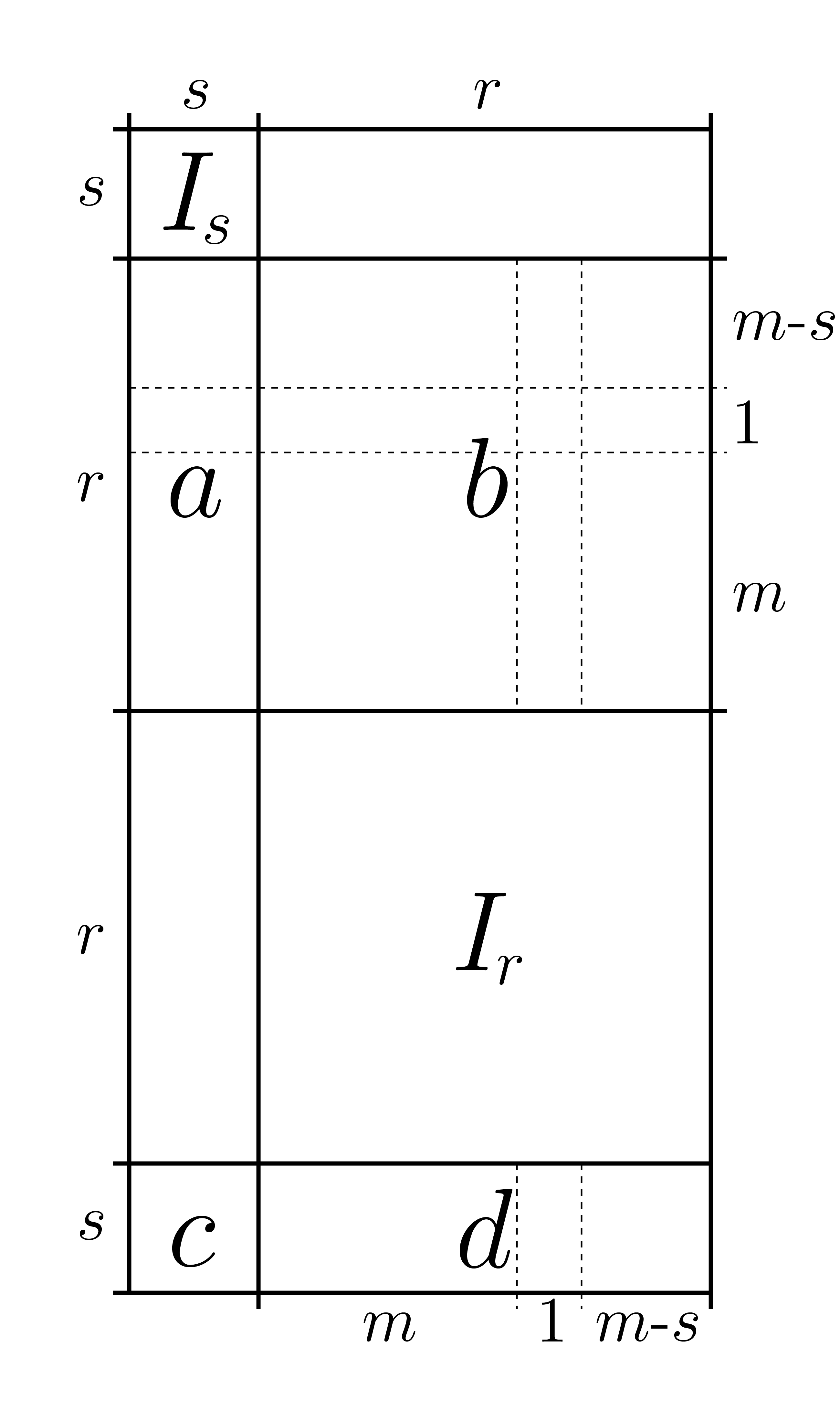
We denote the subspace $\mathcal{F}$ and the matrix representing it (as a column span) by the same symbol. This should not lead to any confusion, since the intended meaning will be clear from the context.

To describe the orthogonal complement of $\mathcal{F}$ in a clear way, we introduce further notations. For the moment, let ${B}$ be an arbitrary matrix with $k$ rows and $l$ columns. We define the involution $\iota$ as follows:

This is the matrix obtained from ${B}$ by reflection at the first angle bisector going through the lower left matrix entry (which is precisely the antidiagonal in the case of a square matrix). Assuming $i\leq k$, we denote by ${B}^{[i]}$ the matrix consisting of the first $i$ rows of $B$ and by ${B}_{[i]}$ the matrix consisting of the last $i$ rows. The $i$th row is denoted by ${B}^{(i)}$. Likewise, assuming $j\leq l$, we write ${}^{[j]}{B}$, ${}_{[j]}{B}$, and ${}^{(j)}{B}$ for the first $j$ columns of $B$, the last $j$ columns, and the $j$th column, respectively. We refer to the single matrix entry in the $i$th row and $j$th column as ${B}_{i,j}$.

We continue to evaluate the conditions of the wedge local model. We are given pairs of subspaces $(\mathcal{F},\mathcal{F}^{\perp})$. Condition (Pi), concerning the stability of $\mathcal{F}$ under the action of $\Pi$, translates into the equation

Here ${R}$ is a square matrix of size $n$, which we subdivide into four blocks as follows:

with ${S}$ a square matrix of size $s$ and ${V}$ a square matrix of size $r$. With respect to the chosen basis, the operator $\Pi$ is given by the matrix

Then (3.3) comes to

Comparison of the matrices yields several identities involving the $a$-, $b$-, $c$-, and $d$-variables. This has to be done carefully since the blocks of the matrices that seem to correspond are of different sizes.

To begin with, we obtain from (3.4) the following identities concerning the blocks of the matrix ${R}$:

Thus, the matrix ${R}$ takes the form

Before examining the remaining blocks of (3.4), we take a look at the wedge condition (W).

Since $\Pi|\mathcal{F}$ is given by the matrix ${R}$, all minors of size $r+1$ of

have to be zero. Note that the first $s$ rows are multiples of the following $s$ rows. Since any minor of size $r+1$ includes at least one pair of such corresponding rows, all these minors are zero.

All minors of size $s+1$ of

have to be zero as well. First, we consider the minors of size $s+1$ obtained by keeping only the rows with row number in $\{s+1,\dots,2s,2s+i\}$ and the columns with column number in $\{1,\dots,s,s+j\}$. Here $i$ and $j$ denote integers with $1\leq i\leq r-s$ and $1\leq j\leq s$. We use Laplace expansion along the last column and calculate

These minors being zero, we get

Next, we consider the minors obtained by keeping the rows $\{s+1,\dots,2s,2s+i\}$ and the columns $\{1,\dots,s,2s+j\}$, with $1\leq i,j\leq r-s$:

These minors being zero, we obtain

Finally, all remaining minors of size $s+1$ are automatically zero now.

The characteristic polynomial of $\Pi|\mathcal{F}$ is given by $\det(T\;{I}_{n}-{R})$, with $R$ as in (3.6). Making use of (3.10), we calculate

which is in accordance with (N4).

We show that the $b$-variables are determined by the $a$-, $c$-, and $d$-variables. For this purpose, we consider the matrix equation ${c}\;{T}+{d}\;{V}={b}_{[s]}$, obtained from the lower right blocks of the matrices in (3.4). Using (3.5), (3.9), and (3.10), the first $s$ columns give

and the last $r-s$ columns give

Combining (3.9)–(3.12) yields the following description of the submatrix ${b}$:

Hence, the ${b}$-variables are determined by the other variables.

With (3.5), the lower left blocks of the matrices in (3.4) give the identity

to which we return later.

The remaining blocks of the matrices in (3.4) give nothing new.

We can deduce further constraints on the $a$-, $c$-, and $d$-variables from (N2), which demands that the maps induced by the lattice inclusions restrict to the considered subspaces.

With respect to the chosen bases, the map corresponding to $\Lambda_{m}\subset\Lambda_{m+1}$ is given by the $2n\times 2n$-matrix

Since this map is required to restrict to $\mathcal{F}\rightarrow\mathcal{F}^{\perp}$, we have to examine the conditions under which ${A}\;\mathcal{F}$ is perpendicular to $\mathcal{F}$. With ${M}$ as in (N3), ${C}:=\mathcal{F}^{\text{{t}}}\;{A}^{\text{{t}}}\;{M}\;\mathcal{F}$ has to be the zero matrix of size $n$. We multiply the matrices on the right hand side. Note the form of the matrix

which suggests that blockwise multiplying becomes easier when subdividing $\mathcal{F}$ into four groups of columns, with the groups consisting of $s$, $m$, $1$, and $m-s$ columns. This partitioning is shown in Fig. 3.1. The symmetry of ${A}^{\text{{t}}}\;{M}$ implies the symmetry of ${C}$, and we obtain ten conditions from the blocks of ${C}$:

1. (C1)

   $0=-{H}_{s}\;{c}+{{a}^{(m-s+1)}}^{\text{{t}}}\;{a}^{(m-s+1)}-{c}^{\text{{t}}}\;{H}_{s}$ ,

2. (C2)

   $0=-{H}_{s}\;^{[m]}{d}+{{a}^{(m-s+1)}}^{\text{{t}}}\;{}^{[m]}{b}^{(m-s+1)}+{{a}_{[m]}}^{\text{{t}}}\;{H}_{m}$ ,

3. (C3)

   $0=-{H}_{s}\;^{(m+1)}{d}+{{a}^{(m-s+1)}}^{\text{{t}}}\;{b}_{m-s+1,m+1}$ ,

4. (C4)

   $0=-{H}_{s}\;{}_{[m-s]}{d}-{{a}^{[m-s]}}^{\text{{t}}}\;{H}_{m-s}+{{a}^{(m-s+1)}}^{\text{{t}}}\;_{[m-s]}{b}^{(m-s+1)}$ ,

5. (C5)

   $0={{}^{[m]}{b}^{(m-s+1)}}^{\text{{t}}}\;{}^{[m]}{b}^{(m-s+1)}+{{}^{[m]}{b}_{[m]}}^{\text{{t}}}\;{H}_{m}+{H}_{m}\;^{[m]}{b}_{[m]}$ ,

6. (C6)

   $0={{}^{[m]}{b}^{(m-s+1)}}^{\text{{t}}}\;{b}_{m-s+1,m+1}+{H}_{m}\;^{(m+1)}{b}_{[m]}$ ,

7. (C7)

   $0=-{{}^{[m]}{b}^{[m-s]}}^{\text{{t}}}\;{H}_{m-s}+{{}^{[m]}{b}^{(m-s+1)}}^{\text{{t}}}\;_{[m-s]}{b}^{(m-s+1)}+{H}_{m}\;{}_{[m-s]}{b}_{[m]}$ ,

8. (C8)

   $0={{b}_{m-s+1,m+1}}^{2}-\pi_{0}$ ,

9. (C9)

   $0=-{{}^{(m+1)}{b}^{[m-s]}}^{\text{{t}}}\;{H}_{m-s}+{b}_{m-s+1,m+1}\;{}_{[m-s]}{b}^{(m-s+1)}$ ,

10. (C10)

    $0=-{{}_{[m-s]}{b}^{[m-s]}}^{\text{{t}}}\;{H}_{m-s}+{{}_{[m-s]}{b}^{(m-s+1)}}^{\text{{t}}}\;_{[m-s]}{b}^{(m-s+1)}-{{H}_{m-s}\;{}_{[m-s]}{b}^{[m-s]}}$ .