On the geometry of broad emission region in quasars
Abstract
We study the geometry of the H broad emission region by comparing the values derived from H through the virial relation with those obtained from the host galaxy luminosity in a sample of 36 low redshift () quasars. This comparison lets us infer the geometrical factor needed to de-project the line-of-sight velocity component of the emitting gas. The wide range of values we found, together with the strong dependence of on the observed line width, suggests that a disc-like model for the broad line region is preferable to an isotropic model, both for radio loud and radio quiet quasars. We examined similar observations of the C iv line and found no correlation in the width of the two lines. Our results indicate that an inflated disc broad line region, in which the Carbon line is emitted in a flat disc while H is produced in a geometrically thick region, can account for the observed differences in the width and shape of the two emission lines.
Keywords:
galaxies: active - galaxies: nuclei - quasars: general - quasars: emission lines1 Introduction
Super-massive black holes (BHs) are found in virtually all massive spheroids (Kormendy & Richstone, 1995). In the Local Universe BH mass measurements can be performed through their imprint on the stellar kinematics (see Ferrarese, 2006 and references therein). The masses of the BHs are correlated with some large scale properties of their host galaxies (Ferrarese & Merritt, 2000; Gebhardt et al., 2000; Magorrian et al., 1998; Marconi & Hunt, 2003; Graham & Driver, 2007). The reader is referred to Graham, (2007) for an up-to-date review on this topic, and to King, (2005) and references therein for interpretative models of the scaling relations.
In Type–1 AGNs the line emission from the gas inside the BH radius of influence is observed. If non-gravitational motions are neglected, the cloud velocity at a given radius is fixed by the BH mass . Emission lines are Doppler broadened according to the gas motions. A simple, isotropic model of the broad line region (BLR) is usually adopted (e.g., Salviander et al., 2007 and the references therein); McLure & Dunlop, (2002), Dunlop et al., (2003) and Laor et al., (2006) found that a disc model is preferable, and Decarli et al., (2008) proved that inclination may explain some peculiar characteristics of the so–called Narrow Line Type–1 AGNs. On the other hand, some authors questioned the underlying virial assumption (Bottorf et al., 1997), at least for some broad emission lines (e.g., Baskin & Laor, 2005). McLure & Dunlop, (2001) and Dunlop et al., (2003), and, more recently, a number of reverberation mapping campaigns (e.g., Metzroth Onken & Peterson, 2006; Bentz et al., 2007; Sergev et al., 2007) found rough agreement between the virial estimate of the BH mass from H width and the one based on the host galaxy luminosities, but the observed dispersions are significant. If the scatter is due to the assumed gas dynamical model, constrains on the BLR geometry can be inferred. Onken et al., (2004) compared the virial estimates of in few, well studied nearby AGNs with the stellar velocity dispersion of their host galaxies. The large offset observed with respect to the relation observed in inactive galaxies suggested that an isotropic geometry is not successful, but they could not put a better constrain on the gas dynamics due to the large uncertainties and the poor statistics. In radio loud quasars (RLQs), the width of the broad lines is roughly correlated to the core-to-lobe power ratio index, (e.g.,Wills & Browne, 1986; Brotherton, 1996; Vestergaard Wilkes & Barthel, 2000). This dependence is usually interpreted in terms of a flat BLR, given that is related to the inclination angle of the jet axis with respect to the line of sight. Whether a flat BLR model can be valid also for radio quiet quasars (RQQs) is still unclear.
| Object | R.A. | Decl. | Radio | log | |||
|---|---|---|---|---|---|---|---|
| name | (J2000.0) | (J2000.0) | [mag] | [mag] | [M⊙] | ||
| (1) | (2) | (3) | (4) | (5) | (6) | (7) | (8) |
| 0054+144 | 00 57 09.9 | +14 46 10 | 0.171 | Q | 15.70 | -22.48 | 8.6 |
| 0100+0205 | 01 03 13.0 | +02 21 10 | 0.393 | Q | 17.51 | -22.00 | 8.4 |
| 0110+297 | 01 13 24.2 | +29 58 15 | 0.363 | L | 17.00 | -22.85 | 8.8 |
| 0133+207 | 01 36 24.4 | +20 57 27 | 0.425 | L | 18.10 | -22.69 | 8.7 |
| 3C48 | 01 37 41.3 | +33 09 35 | 0.367 | L | 16.20 | -24.76 | 9.8 |
| 0204+292 | 02 07 02.2 | +29 30 46 | 0.109 | Q | 16.80 | -22.80 | 8.8 |
| 0244+194 | 02 47 40.8 | +19 40 58 | 0.176 | Q | 16.66 | -22.29 | 8.5 |
| 0624+6907 | 06 30 02.5 | +69 05 04 | 0.370 | Q | 14.20 | -24.53 | 9.6 |
| 07546+3928 | 07 58 00.0 | +39 20 29 | 0.096 | Q | 14.36 | -24.08 | 9.4 |
| US1867 | 08 53 34.2 | +43 49 02 | 0.513 | Q | 16.40 | -23.39 | 9.1 |
| 0903+169 | 09 06 31.9 | +16 46 11 | 0.412 | L | 18.27 | -22.76 | 8.8 |
| 0923+201 | 09 25 54.7 | +19 54 05 | 0.190 | Q | 15.80 | -22.15 | 8.4 |
| 0944.1+1333 | 09 46 52.0 | +13 20 26 | 0.131 | Q | 16.05 | -23.23 | 9.0 |
| 0953+415 | 09 56 52.4 | +41 15 22 | 0.234 | Q | 15.30 | -22.24 | 8.4 |
| 1001+291 | 10 04 02.5 | +28 55 35 | 0.330 | Q | 15.50 | -23.42 | 9.1 |
| 1004+130 | 10 07 26.1 | +12 48 56 | 0.240 | L | 15.20 | -23.10 | 8.9 |
| 1058+110 | 11 00 47.8 | +10 46 13 | 0.423 | L | 17.10 | -22.46 | 8.6 |
| 1100+772 | 11 04 13.7 | +76 58 58 | 0.315 | L | 15.72 | -23.55 | 9.1 |
| 1150+497 | 11 53 24.4 | +49 31 09 | 0.334 | L | 17.10 | -23.66 | 9.2 |
| 1202+281 | 12 04 42.1 | +27 54 11 | 0.165 | Q | 15.60 | -22.40 | 8.6 |
| 1216+069 | 12 19 20.9 | +06 38 38 | 0.331 | Q | 15.65 | -22.29 | 8.5 |
| Mrk0205 | 12 21 44.0 | +75 18 38 | 0.071 | Q | 15.24 | -22.63 | 8.7 |
| 1222+125 | 12 25 12.9 | +12 18 36 | 0.411 | L | 17.86 | -23.22 | 9.0 |
| 1230+097 | 12 33 25.8 | +09 31 23 | 0.415 | Q | 16.15 | -23.89 | 9.3 |
| 1307+085 | 13 09 47.0 | +08 19 49 | 0.155 | Q | 15.10 | -21.89 | 8.3 |
| 1309+355 | 13 12 17.8 | +35 15 21 | 0.184 | L | 15.64 | -23.29 | 9.0 |
| 1402+436 | 14 04 38.8 | +43 27 07 | 0.323 | Q | 15.62 | -22.96 | 8.8 |
| 1425+267 | 14 27 35.5 | +26 32 14 | 0.366 | L | 15.68 | -23.04 | 8.9 |
| 1444+407 | 14 46 45.9 | +40 35 06 | 0.267 | Q | 15.70 | -22.66 | 8.7 |
| 1512+37 | 15 14 43.0 | +36 50 50 | 0.371 | L | 16.27 | -23.09 | 8.9 |
| 3C323.1 | 15 47 43.5 | +20 52 17 | 0.266 | L | 16.70 | -23.06 | 8.9 |
| 1549+203 | 15 52 02.3 | +20 14 02 | 0.250 | Q | 16.40 | -21.86 | 8.3 |
| 1635+119 | 16 37 46.5 | +11 49 50 | 0.146 | Q | 16.50 | -22.40 | 8.6 |
| 3C351 | 17 04 41.4 | +60 44 31 | 0.372 | L | 15.28 | -23.55 | 9.1 |
| 1821+643 | 18 21 57.3 | +64 20 36 | 0.297 | Q | 14.10 | -24.44 | 9.6 |
| 2141+175 | 21 43 35.5 | +17 43 49 | 0.213 | L | 15.73 | -23.13 | 8.9 |
| 2201+315 | 22 03 15.0 | +31 45 38 | 0.295 | L | 15.58 | -24.28 | 9.5 |
| 2247+140 | 22 50 25.3 | +14 19 52 | 0.235 | L | 16.93 | -23.11 | 8.9 |
H is the best studied emission line for low-redshift objects, while Mg iiλ2798 and C ivλ1549 are often chosen for higher redshift (e.g. McLure & Jarvis, 2002, Peterson et al., 2004, Kaspi et al., 2005 and 2007, Peng et al., 2006), since they fall in the optical range for and respectively. Mg ii and H widths are well correlated (Salviander et al., 2007), while C iv line shows systematic deviances from the H values (Baskin & Laor, 2005, Vestergaard & Peterson, 2006). Labita et al., (2006) studied derived from C iv width as a function of a -based for a sample of low-redshift quasars. They found a significantly better correlation than that reported by McLure & Dunlop, (2001) for H data.
In this paper we study the BLR geometry and gas dynamics by comparing the values derived from H broad emission with those obtained from the host galaxy luminosity in a sample of 36 low redshift () quasars. The sample is selected in order to provide similar numbers of RLQs and RQQs, so that conclusions on the geometry of the BLR can be drawn for both classes. Comparing our results with those of Labita et al., (2006), based on C iv line, we sketch a picture of the dynamics of the gas around the BH. Note that since the dynamical model of the BLR is assumed to be independent of redshift, we also test the evolution of the BH–host galaxy relations.
We define our sample in section 2. Data sources are summarized in section 3. Data analysis is described in section 4. We then discuss our results (section 5). The sketch of the broad line region dynamics is presented in section 6. Throughout the paper we adopt a concordance cosmology with km/s/Mpc, and . We converted the results of other authors to this cosmology when adopting their relations and data.
2 The sample
We selected all quasars in the Veron-Cetty & Veron, (2006) catalogue that have been imaged by HST-WFPC2 (exposure time s). The host galaxies are required to be elliptical, and therefore the bulge component practically coincides with the whole galaxy. We considered all the quasars with , so that the Hλ 4861–[O iii]λλ 4959,5007 lines are present in the optical spectra. For their observability from the Northern hemisphere, we selected only objects with . The entire sample thus consists of 53 targets. 12 of them have available spectra in the Sloan Digital Sky Survey (SDSS; see section 3.2). Other 32 spectra were taken on purpose at the Asiago Observatory (see section 3.2), including 6 targets already observed by the SDSS. Two observed targets were then excluded from our analysis: 0903+169 (RQQ) because of the low signal to noise ratio in the available spectrum, and 0923+201 (RLQ) because of the peculiar, composite profile of its broad lines, possibly due to the interaction with a nearby galaxy (see McLeod & Rieke, 1994; Bennert et al., 2007). Thus per cent of the sample was covered, including 16 RLQs and 20 RQQs. Table 1 summarizes the main properties of the objects in our sample.
3 Data sources
3.1 Host galaxy magnitudes and
The host galaxy apparent magnitudes were taken from the literature (Hooper et al., 1997; Boyce et al., 1998; Kirhakos et al., 1999; Pagani et al., 2003; Dunlop et al., 2003; Labita et al., 2006) or converted from published or luminosities (Bahcall et al., 1997; Hamilton et al., 2002; Floyd et al., 2004). Corrections for galactic extinction are from Schlegel et al., (1998). To perform colour and -correction transformations we adopted an elliptical galaxy template (Mannucci et al. 2001), assuming that the host galaxies are dominated by old stellar population. The -correction for an elliptical galaxy at observed in the -band is mag. The passive evolution of the host galaxies follows Bressan, Chiosi & Fagotto (1994), as discussed in Labita et al., (2006). Typical corrections for the passive evolution are mag. The resulting -band absolute magnitudes of the host galaxies are given in table 1.
We use the relationship obtained by Bettoni et al., (2003), corrected for the chosen cosmology, in order to estimate from the host galaxy luminosity:
| (1) |
where is the absolute magnitude of the bulge component of the host galaxy. The rms of this fit is . Table 1 also lists the resulting values.
3.2 Spectroscopic observations
32 optical spectra were taken with the m Cima Ekar telescope at the Asiago Observatory. The Asiago Faint Object Spectrograph Camera was mounted in longslit spectroscopy configuration with grisms n. 4, 7 and 8, yielding spectral resolutions of , and ( slit) in the spectral range – Å, – Å and – Å respectively (pxl = , and Å/pxl). At Å the spectral instrumental resolutions are , and Å, tight enough to distinguish prominent H narrow emission from the broad one.
The standard IRAF procedure was adopted in the data reduction. The
ccdred package was employed to perform bias subtraction, flat
field correction, image alignment and combination. Cosmic rays were
eliminated by combining 3 or more exposures of the same objects, and
applying crreject algorithm while averaging. When only one or
two bidimensional spectra were available, we applied
cosmicrays task in the crutils package. In order to
prevent the task from altering the narrow component of emission
lines, we masked the central region of our bidimensional spectra.
The spectra extraction, the background subtraction and the
calibrations both in wavelength and in flux were performed with
doslit task in kpnoslit package, using a Hg-Cd and Ne
lamps and spectrophotometric standard stars as reference. Wavelength
calibration residuals are around Å (sub-pixel), thus
implying a negligible ( per cent) error on redshift estimates.
Absolute calibration of spectra was corrected through the photometry
of field stars, by comparing corollary imaging with Johnson’s R and
V filters to the magnitudes published in the U.S. Naval Observatory
catalogue. The uncertainty in the flux calibration is mag.
Galactic extinction was accounted for according to Schlegel, et al.
(1998) , assuming .
Table 2 summarizes the observed targets.
| Object | z | Available | Date | Seeing | |
|---|---|---|---|---|---|
| name | [mag] | spectra | [arcsec] | ||
| (1) | (2) | (3) | (4) | (5) | (6) |
| 0054+144 | 0.171 | 15.70 | A4,S | 13/09/06 | 1.4 |
| 0100+020 | 0.393 | 16.39 | A4,H | 18/09/07 | n/a |
| 0110+297 | 0.363 | 17.00 | A4 | 09/12/05 | 2.1 |
| 0133+207 | 0.425 | 18.10 | A4,H | 27/11/06 | 2.0 |
| 3C48 | 0.367 | 16.20 | A4 | 11/12/05 | n/a |
| 0204+2916 | 0.109 | 16.80 | A4 | 15/10/06 | 1.7 |
| 0244+194 | 0.176 | 16.66 | A4 | 16/10/06 | 1.7 |
| 0624+6907 | 0.370 | 14.20 | A4,H | 27/10/06 | 2.6 |
| 07546+3928 | 0.096 | 14.36 | A4 | 24/12/05 | 1.9 |
| US1867 | 0.513 | 16.40 | A4,S,H | 27/11/06 | 1.3 |
| 0944.1+1333 | 0.131 | 16.05 | A4 | 25/04/06 | 2.4 |
| 0953+415 | 0.234 | 15.30 | A4 | 07/02/06 | 3.1 |
| 1001+291 | 0.330 | 15.50 | A4 | 19/02/06 | 2.4 |
| 1004+130 | 0.240 | 15.20 | A4,S | 07/03/06 | 2.2 |
| 1058+110 | 0.423 | 17.10 | A4,S | 26/04/06 | 2.0 |
| 1100+772 | 0.315 | 15.72 | A4 | 08/03/06 | 2.7 |
| 1202+281 | 0.165 | 15.60 | A4,H | 20/02/06 | 2.3 |
| 1216+069 | 0.331 | 15.65 | A8,H | 12/04/07 | 1.9 |
| Mrk0205 | 0.071 | 15.24 | A7,H | 11/04/07 | 1.6 |
| 1307+085 | 0.155 | 15.10 | A7,H | 24/04/07 | 1.6 |
| 1309+355 | 0.184 | 15.64 | A4,H | 20/02/06 | 2.4 |
| 1402+436 | 0.323 | 15.62 | A4,S | 07/03/06 | 3.6 |
| 1425+267 | 0.366 | 15.68 | A4,H | 20/02/06 | 2.9 |
| 3C323.1 | 0.266 | 16.70 | A7,H | 24/04/07 | 1.4 |
| 1549+203 | 0.250 | 16.40 | A4 | 23/04/06 | 2.0 |
| 1635+119 | 0.146 | 16.50 | A4 | 31/05/06 | 2.8 |
| 1821+643 | 0.297 | 14.10 | A4,H | 15/12/06 | 2.1 |
| 2141+175 | 0.213 | 15.73 | A4,H | 15/12/06 | 1.9 |
| 2201+315 | 0.295 | 15.58 | A4,H | 15/12/06 | 1.5 |
| 2247+140 | 0.235 | 16.93 | A4,S,H | 12/09/06 | 1.5 |
The SDSS Data Release 5 (Adelman-McCarthy, et al., 2007) provides spectra for 12 quasars in our sample. SDSS spectra have and a spectral range between and Å. Uncertainties on wavelength calibration amount to Å, while flux calibration formal errors account to 5 per cent. We re-observed six of these objects (0054+144, US1867, 1004+130, 1058+110, 1402+436, 2247+140) in order to perform a comparison. Both the specific fluxes at 5100 Å and the H broad line widths are in good agreement. Due to their better spectral resolution, we will consider only the SDSS spectra of these objects in our analysis.
4 The virial determination of
In the virial assumption, if the velocity of a particle orbiting at a certain radius around the BH is known, the mass of the BH is simply:
| (2) |
In Type-1 AGNs expression (2) can be evaluated at the characteristic radius of the BLR, , which can be measured almost directly with the reverberation mapping technique (Blandford & McKee, 1982). Kaspi et al., (2000) found that the nuclear monochromatic luminosity, , is correlated with by , with depending on the considered emission line. The broad line width is used to estimate . According to the adopted dynamical model,
| (3) |
where is a geometrical factor11 1 The reader should notice that different definitions for are available in literature: Vestergaard & Peterson, (2006) and Collin et al., (2006) use . and the FWHM is expressed in velocity units. If the gas moves isotropically, a gaussian line shape is observed, with . If a rotational component is present, an axial symmetry is introduced, and depends on the inclination angle :
| (4) |
where is the angle between the line of sight and the rotation axis, and and are parameters accounting for the importance of the disc and isotropic components respectively. The reader is referred to McLure & Dunlop, (2001), Labita et al., (2006), Collin et al., (2006) and Decarli et al., (2008) for detailed discussions on this topic. Since value is generally unknown, one defines the Virial Product as:
| (5) |
corresponding to if is taken unitary. Thus, an estimate of requires measures of the monochromatic luminosity , of the line width and independently of .

4.1 The monochromatic luminosity
The continuum luminosity was calculated as follows: Rest-frame spectral continua were fitted with a power-law (see figure 1). The key-point is to avoid contaminations due to various emission features, especially to broad Fe ii bands. Typical rest-frame fitted regions are around 2610, 3030, 4030, 4190, 5080 Å and in the 5450-5720 Å range. The 5100 Å region is generally free from contaminations and can be easily fitted. The resulting fit function was computed at 5100 Å, thus providing (5100 Å). We corrected for the host galaxy contamination by computing the fraction of its flux within the slit, on the basis of the nucleus and host galaxy luminosities and the effective radius estimates available from the literature, and following the recipe adopted by Sbarufatti et al., (2006). The average correction is dex.
| Object | z | Data | |||
|---|---|---|---|---|---|
| name | set | [erg/s/cm2/Å] | [erg/s] | [cm] | |
| (1) | (2) | (3) | (4) | (5) | (6) |
| 0054+144 | 0.171 | S | -14.9 | 44.7 | 17.2 |
| 0100+0205 | 0.393 | A4 | -15.6 | 44.9 | 17.3 |
| 0110+297 | 0.363 | A4 | -15.5 | 44.7 | 17.2 |
| 0133+207 | 0.424 | A4 | -15.6 | 44.7 | 17.2 |
| 3C48 | 0.369 | A4 | -14.9 | 45.4 | 17.6 |
| 0204+292 | 0.110 | A4 | -15.1 | 44.2 | 16.8 |
| 0244+194 | 0.174 | A4 | -15.1 | 44.7 | 17.2 |
| 0624+6907 | 0.370 | A4 | -14.5 | 46.1 | 18.1 |
| 07546+3928 | 0.096 | A4 | -14.2 | 44.7 | 17.2 |
| US1867 | 0.515 | S | -15.3 | 45.3 | 17.6 |
| 0944.1+1333 | 0.134 | A4 | -14.8 | 44.5 | 17.1 |
| 0953+415 | 0.235 | A4 | -14.8 | 45.6 | 17.8 |
| 1001+291 | 0.330 | A4 | -14.9 | 45.1 | 17.5 |
| 1004+130 | 0.241 | S | -14.7 | 45.2 | 17.5 |
| 1058+110 | 0.423 | S | -15.9 | 44.6 | 17.1 |
| 1100+772 | 0.311 | A4 | -14.4 | 45.8 | 17.9 |
| 1150+497 | 0.334 | S | -15.6 | 44.6 | 17.1 |
| 1202+281 | 0.165 | A4 | -15.3 | 44.6 | 17.1 |
| 1216p069 | 0.331 | A8 | -14.7 | 45.6 | 17.8 |
| Mrk0205 | 0.071 | A7 | -14.7 | 44.5 | 17.0 |
| 1222+125 | 0.412 | S | -15.6 | 44.8 | 17.2 |
| 1230+097 | 0.416 | S | -15.2 | 45.2 | 17.5 |
| 1307p085 | 0.155 | A7 | -15.0 | 45.3 | 17.6 |
| 1309+355 | 0.184 | A4 | -14.7 | 44.4 | 17.0 |
| 1402+436 | 0.323 | S | -14.7 | 45.4 | 17.7 |
| 1425+267 | 0.366 | A4 | -15.4 | 45.2 | 17.5 |
| 1444+407 | 0.267 | S | -14.9 | 45.1 | 17.4 |
| 1512+37 | 0.371 | S | -15.3 | 45.0 | 17.4 |
| 3C323.1 | 0.266 | A7 | -15.2 | 45.2 | 17.5 |
| 1549+203 | 0.253 | A4 | -15.2 | 44.8 | 17.3 |
| 1635+119 | 0.148 | A4 | -15.4 | 42.2 | 15.5 |
| 3C351 | 0.372 | S | -14.7 | 45.6 | 17.8 |
| 1821+643 | 0.297 | A4 | -14.2 | 46.1 | 18.1 |
| 2141+175 | 0.211 | A4 | -15.0 | 45.0 | 17.4 |
| 2201+315 | 0.295 | A4 | -14.9 | 45.4 | 17.7 |
| 2247+140 | 0.235 | S | -15.3 | 44.6 | 17.1 |
4.2 Line width measurements
The observed H broad component is usually contaminated by other spectral features, in particular by blended Fe ii multiplets, the H narrow component and the [O iii]λλ4959,5007 lines.
Strong Fe ii emissions are commonly detected in quasar spectra at 4400-4750 and 5150-5450 Å, and weaker blended features are found at 4800-5000 Å. A common practice to remove this contamination (e.g., Boroson & Green, 1992; Marziani et al., 2003; Salviander et al., 2007; McGill et al., 2007) is to adopt the spectrum of I Zw001 as a template of the Fe ii emission, due to the intensity and narrowness of the Fe ii lines. Since the relative intensities of the various Fe ii features may differ from a quasar to another (see, for example, table 7 in Phillips, 1978), we preferred a more conservative approach: we modeled the Fe ii emission as a simple power-law fitted at and Å, and subtracted it from the observed spectrum. The reliability of this procedure is discussed in appendix A.1.
Since most of our objects have the H red wing contaminated by [Fe viii]λ4894, Fe iiλλ4924,5018 and [O iii]λλ4959,5007 lines, a reliable study of the broad line asymmetries is extremely hard to achieve, and is strongly dependent on the procedure adopted in removing these contaminations. We preferred to set the same peak wavelength for both the gaussian curves, thus neglecting line asymmetries. In appendix A.2 we discuss how the use of a different fitting function, sensitive to the asymmetries in the line profile, does not affect the estimates of the line width in a significant way.
The fit procedure was preferred to the width measurement directly applied to the observed data (without any fit; see for example Collin et al., 2006) since: 1) it is applicable also to low signal-to-noise spectra; 2) it does not require an accurate modeling of the narrow component; 3) it is reliable even in the largest tails, where contaminations by other emission or absorption features may be relevant.
We derived the FWHM and the second moment of the line, , from
the fitted profile. Both FWHM and are corrected for
instrumental spectral resolution. The ratio between FWHM and
is used to study the shape of the line, as discussed in
section 5.1. According to Collin et al., (2006),
could be preferred to FWHM as a line width indicator, since it is
strongly dependent on the line wings, i.e., to the kinematics of the
innermost clouds. On the other hand, is very sensitive to
contaminations and to the adopted Fe ii subtraction. Therefore, we
will use the FWHM in the estimates, and consider
only in the study of the line shape. Figure 2 offers
an example of the fitting procedure, applied to 1821+643. Plots for
the whole sample are available in electronic form at
www.dfm.uninsubria.it/astro/caqos/index.html. Our H width
estimates are listed in table 4. Typical uncertainties
in the FWHM values due to the fit procedure are per cent of
the line width.

| Object | Data | FWHM | FWHM | ||
|---|---|---|---|---|---|
| name | set | [Å] | [Å] | [km/s] | [km/s] |
| (1) | (2) | (3) | (4) | (5) | (6) |
| 0054+144 | S | 134 | 57 | 8220 | 3520 |
| 0100+0205 | A4 | 79 | 35 | 4870 | 2160 |
| 0110+297 | A4 | 100 | 40 | 6150 | 2440 |
| 0133+207 | A4 | 143 | 53 | 8850 | 3260 |
| 3C48 | A4 | 65 | 39 | 4010 | 2370 |
| 0204+292 | A4 | 145 | 67 | 8960 | 4110 |
| 0244+194 | A4 | 76 | 36 | 4680 | 2220 |
| 0624+6907 | A4 | 59 | 32 | 3630 | 1940 |
| 07546+3928 | A4 | 50 | 28 | 3110 | 1750 |
| US1867 | S | 37 | 31 | 2280 | 1900 |
| 0944.1+1333 | A4 | 52 | 30 | 3230 | 1850 |
| 0953+415 | A4 | 58 | 47 | 3610 | 2890 |
| 1001+291 | A4 | 32 | 26 | 1980 | 1610 |
| 1004+130 | S | 98 | 50 | 6010 | 3060 |
| 1058+110 | S | 121 | 48 | 7460 | 2950 |
| 1100+772 | A4 | 113 | 58 | 6980 | 3550 |
| 1150+497 | S | 63 | 28 | 3870 | 1750 |
| 1202+281 | A4 | 84 | 57 | 5190 | 3510 |
| 1216+069 | A8 | 83 | 50 | 5110 | 3080 |
| Mrk0205 | A7 | 53 | 34 | 3270 | 2100 |
| 1222+125 | S | 122 | 56 | 7530 | 3430 |
| 1230+097 | S | 77 | 41 | 4770 | 2540 |
| 1307+085 | A7 | 57 | 27 | 3520 | 1670 |
| 1309+355 | A4 | 72 | 44 | 4430 | 2720 |
| 1402+436 | S | 45 | 33 | 2760 | 2030 |
| 1425+267 | A4 | 131 | 73 | 8090 | 4530 |
| 1444+407 | S | 44 | 27 | 2690 | 1650 |
| 1512+37 | S | 144 | 52 | 8910 | 3210 |
| 3C323.1 | A7 | 77 | 37 | 4760 | 2290 |
| 1549+203 | A4 | 30 | 20 | 1880 | 1230 |
| 1635+119 | A4 | 92 | 46 | 5700 | 2870 |
| 3C351 | S | 150 | 63 | 9260 | 3870 |
| 1821+643 | A4 | 78 | 34 | 4820 | 2090 |
| 2141+175 | A4 | 84 | 36 | 5180 | 2230 |
| 2201+315 | A4 | 49 | 28 | 3020 | 1720 |
| 2247+140 | S | 52 | 22 | 3180 | 1330 |
5 Discussion
5.1 H line width and shape
The mean value and rms of the H FWHM distribution are:
A different distribution of FWHM is observed between RLQs and RQQs, in the sense that the former ones show, on average, wider lines than the latter. This difference may be intrinsic, the velocity of the gas in RLQs being actually larger than in RQQs, independently on the BLR geometry. Indeed, as we will notice later, a bias towards the high–mass end of the distribution occurs for RLQs (partially related to the Malmquist bias, since the average redshift of our sample RLQs is higher than that of RQQs). Otherwise, in the prospective of a disc–like broad line region, different average inclination angles may account for the different distributions in the FWHM values. This may be achieved assuming that, while RLQs have , the RQQs are biased towards lower inclination angles, e.g. . Such a bias has been already hypothesized by some authors (e.g., Francis et al., 2000), but its occurrence is still debated (see, for example, Kotilainen et al., 2007).
The comparison between H FWHM and illustrates some general properties of the line shape (see figure 3). A single gaussian has FWHM/. The single gaussian case (upper dashed line) represents an upper limit for FWHM. Only few H data have FWHM (lower dashed line). Collin et al., (2006) suggested a bimodality in the FWHM vs relation, with a break when km/s. We argue that such a behaviour is mainly due to the fit procedure adopted by those authors: When the H width is estimated directly on the observed spectrum, cannot be integrated up to infinity, because of He iiλ4686, [Ar iv]λλ4711,4740 and Fe ii contaminations. Integral truncation leads to underestimates of the largest line widths: For a single gaussian curve, the deviation is significant when times the width of the truncation interval. Typically, H can be studied only in the first 80 Å bluewards. That means, Å are underestimated. In disagreement with Collin’s results, our fit-based FWHM to ratio is found to be constant all over the observed values of . No systematic difference is reported in the FWHM/ ratio of RLQs and RQQs.

5.2 Broad Line Region radii
Kaspi et al. (2000) found that the radius of the broad line region, as estimated by the reverberation mapping, is related to the continuum monochromatic luminosity . An increasing body of measurements is now available for H time lags (e.g. Kaspi et al., 2000, Suganuma et al., 2006, Bentz et al., 2006). Following Kaspi et al., (2005) we adopt:
| (6) |
The average characteristic radius for H is:
where the error is the standard deviation.
5.3 Redshift dependence of the – relation
Our work is centered on the comparison between the Virial Products (equation 5) and the evaluated from the host galaxy luminosity. Woo et al., (2006) and Treu et al., (2007) proposed that the –bulge relations change significantly even at . On the other hand, Lauer et al., (2007) showed that such a result is probably due to a statistical bias. Owing to the steepness of the bright end of galaxy luminosity function, very high mass black holes are more commonly upper residuals of the –host luminosity, rather than being hosted by correspondingly very massive galaxies. Thus, when a luminosity cutoff is adopted (typically due to sensitivity limits, when observing at high redshift), the expected from – relation tends to be lower than the real one. Since the geometrical factor is supposed to be independent of redshift, we can directly test the evolution of the Bettoni relation (equation 1) checking the redshift dependence of VPs, host absolute magnitudes and their ratios. We consider here only the objects the host galaxies of which have similar luminosities, namely, the (15) objects with mag, since they are roughly well distributed along the considered redshift range. While an overall slight increase in the VPs is found with redshift (possibly due to Malmquist bias), data dispersion largely exceeds the effect reported in Woo et al., (2006) and Treu et al., (2007), our objects being consistent with a no-evolution scenario. A lower scatter is observed for C iv data taken from Labita et al., (2006) (see section 5.5). Applying the same argument, no significant redshift dependence is found in the VP-to-host galaxy luminosity ratios, the probability of null correlation exceeding 30 per cent.
5.4 Spectroscopic Virial Products vs Imaging estimates
| Object | z | log VP (H) | |
|---|---|---|---|
| name | [M⊙] | ||
| (1) | (2) | (3) | (4) |
| 0054+144 | 0.171 | 8.9 | 0.7 |
| 0100+0205 | 0.393 | 8.6 | 0.8 |
| 0110+297 | 0.363 | 8.6 | 1.1 |
| 0133+207 | 0.424 | 9.0 | 0.6 |
| 3C48 | 0.368 | 8.7 | 3.0 |
| 0204+292 | 0.110 | 8.6 | 1.1 |
| 0244+194 | 0.174 | 8.4 | 1.1 |
| 0624+6907 | 0.370 | 9.1 | 1.8 |
| 07546+3928 | 0.096 | 8.0 | 4.6 |
| US1867 | 0.515 | 8.2 | 2.6 |
| 0944.1+1333 | 0.134 | 7.9 | 3.4 |
| 0953+415 | 0.235 | 8.8 | 0.7 |
| 1001+291 | 0.330 | 7.8 | 4.4 |
| 1004+130 | 0.241 | 9.0 | 0.9 |
| 1058+110 | 0.423 | 8.7 | 0.8 |
| 1100+772 | 0.311 | 9.5 | 0.6 |
| 1150+497 | 0.334 | 8.1 | 3.1 |
| 1202+281 | 0.165 | 8.4 | 1.2 |
| 1216+069 | 0.331 | 9.1 | 0.5 |
| Mrk0205 | 0.071 | 8.0 | 2.2 |
| 1222+125 | 0.412 | 8.8 | 1.0 |
| 1230+097 | 0.416 | 8.8 | 1.7 |
| 1307+085 | 0.155 | 8.5 | 0.7 |
| 1309+355 | 0.184 | 8.1 | 2.2 |
| 1402+436 | 0.323 | 8.5 | 1.5 |
| 1425+267 | 0.366 | 9.2 | 0.7 |
| 1444+407 | 0.267 | 8.2 | 1.8 |
| 1512+37 | 0.371 | 9.2 | 0.7 |
| 3C323.1 | 0.266 | 8.8 | 1.1 |
| 1549+203 | 0.253 | 7.5 | 2.4 |
| 1635+119 | 0.148 | 6.9 | 0.6 |
| 3C351 | 0.372 | 9.6 | 0.5 |
| 1821+643 | 0.297 | 9.4 | 1.3 |
| 2141+175 | 0.211 | 8.7 | 1.3 |
| 2201+315 | 0.295 | 8.4 | 3.2 |
| 2247+140 | 0.235 | 8.0 | 2.7 |
We are now ready to compare the Virial Products to the BH masses as estimated from the host galaxy luminosity. VPs and values are listed in table 5. Typical uncertainties on VPs and are dex, due mainly to the scatter in the – and – relations. The comparison is shown in figure 4. Our data show no correlation: The probability of non-correlation is per cent, with a Spearman’s rank coefficient of and a residual standard deviation of dex. The mean value of is . The dispersion in our data reflects the values obtained in the same way by Dunlop et al., (2003) (see their figure 13).

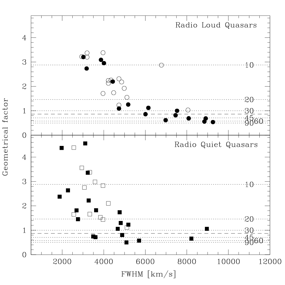
We study now the geometrical factor of our sample quasars separately according to radio loudness. Indeed, indications that RLQs may have flat BLRs have been already reported (in particular, the rough dependence of on the FWHM of H: Wills & Browne, 1986; Brotherton, 1996; Vestergaard Wilkes & Barthel, 2000), while not so much is known about RQQs. In RLQs, the factor is found to be strongly dependent on the FWHM of the lines, as shown in figure 5, upper panel. We note that such a relation show significantly less dispersion than the FWHM– published for similar samples (e.g., see figure 4 in Brotherton, 1996). Some authors proposed the existence of two different populations with different FWHM ranges and average (Sulentic et al., 2000; Collin et al., 2006). Our data confirm this result, even if a continuous trend rather than a strict bimodality seems to be present. All the objects with FWHM km/s have , the value of rapidly decreasing with FWHM. According to equation 3, such a trend would be expected only if is not fixed, given . This reinforces the idea that RLQs have disc–like BLRs.
A similar picture is observed for RQQs, even if a larger dispersion is found (see, for comparison, McLure & Dunlop, 2002). The occurrence of two populations is still clear: at FWHM km/s all but two targets have , while only few targets with FWHM km/s have . This rules out that the BLR is isotropic even in RQQs.
We simulated the –FWHM relation in the hypothesis of a thin disc BLR (figure 6). We assumed a gaussian distribution of the uncertainties for FWHM, VP and , mimicking the uncertainties in the adopted fitting techniques and scaling relations. We then assumed that all the quasars have purely disc-like BLRs, with a fixed rotational velocity . Fitting our data with a hyperbole (see eq. 3), we found and km/s for RLQs and RQQs respectively. The variable was let free to vary from to . The angle was fixed to and for RLQs and RQQs respectively, in order to match the median value of the observed distributions. The simulated values are overplotted to the measures presented in figure 5 for a comparison. We also plotted the two lines corresponding to the expected values of if uncertainties were negligible. Both RLQs and RQQs are well described with a disc model of the BLR, with the former ones showing larger than the latter ones. This difference cannot be explained in terms of a different range of , and – as we noted in section 5.1 – may be the effect of a selection bias, in the sense that the RLQs in our sample have higher average than RQQs. Concerning the different FWHM distributions of RLQs and RQQs, our simulation cannot rule out a dependence on the adopted range of , as suggested by the the estimates of based on the distributions of . Extending this technique on a larger sample is needed to properly address this topic.

5.5 Comparison between C iv and H lines
We now want to compare the H properties with those of the C ivλ 1549 line. We will refer to the C iv data in Labita et al., (2006), who used the C iv line in order to measure the VPs of 29 low-redshift quasars observed with HST-FOS. 16 out of 29 objects in that work are also present in our sample. The average C iv FWHM and its standard deviation are:
C iv FWHMs show smaller dispersion and a smaller mean value than H ones. This is remarkable: the C iv line requires higher ionization potential than H. If the virial hypothesis is valid and a simple photoionization model is assumed, C iv emission should show lower radii and, accordingly to equation 2, higher velocities. In section 6 we will show how this point can be interpreted in terms of different thickness of the BLR disc at C iv and H radii. Figure 7 shows the comparison between C iv and H FWHMs for the objects common to both our and Labita’s studies. No correlation is apparent (the probability of non-correlation being up to per cent), as already noticed for different samples by Baskin & Laor, (2005) (81 quasars) and Vestergaard & Peterson, (2006) (32 quasars; see their figure 10). We argue that the FWHM values of the two lines are intrinsically different.

As in the H case (figure 3), we now consider the comparison between C iv FWHM and . Even if we sampled only a small range of values, the data from the two lines clearly fill different regions of the (FWHM, ) plane. Since the fitting procedure is similar, we can rule out a systematic effect due to the width estimate algorithm. Thus, we argue that C iv and H broad lines have intrinsically different shapes, the C iv departing more from the isotropic (gaussian) case than H.
The continuum monochromatic luminosity at 1350 Å is also considered for the objects belonging to the sample of Labita et al., (2006). We use this information in order to estimate for C iv data, by means of the radius-luminosity relation published by Kaspi et al., (2007):
| (7) |
This is the first available relation based on reverberation mapping studies of the C iv lines. However, it is based only on 8 sources, thus the slope and offset of the relation shall need some tuning when other data will be available. The average (C iv) result:
The (C iv) is found to be systematically ( times) smaller than (H), but we warn the reader that the scatter due to the – relations is severe. Values of (C iv) smaller than (H) are consistent with simple photoionization models: The C iv line is a higher ionization line than H, thus it should be emitted in an inner region. Such a difference, if confirmed, should be taken into account when referring to previous works where the (H) was used as a surrogate for (C iv).
Following the steps traced in section 5.4, we estimate the VPs also for the C iv data. Carbon VPs are well correlated with imaging BH mass estimates (see figure 4): The probability of non-correlation is per cent with a Spearman’s rank coefficient of and a residual standard deviation of dex, comparable with the dispersion in the luminosity-radius relations. Even considering only the common sample, the probability of non-correlation for C iv and H data is and per cent respectively. The mean value of for C iv data amounts to . This value is times larger than the value obtained by Labita et al., (2006) on the same data, since they adopted a different – relation (Pian Falomo & Treves, 2005), which provided an estimate of the H broad-line radius rather than the C iv one. The dependence on FWHM is observed also in C iv data (see figures 5 and 6). No value deduced from C iv line is found to be consistent with an isotropic model of the BLR. The –FWHM plot for C iv–based data is fully consistent with a disc-like BLR, both for RLQs and RQQs. In the average value of , the C iv line appears farther from the isotropic case than the H, both being inconsistent with isotropy.
The formally better correlation of imaging-based BH mass estimates with VPs for C iv line rather than for H suggests that the former could be preferable as a mass indicator than H, as already proposed by Vestergaard & Peterson, (2006) and references therein. If confirmed, this disagrees with recent claims (Baskin & Laor, 2005; Sulentic et al., 2007), in which the average blueshift of the high-ionization lines with respect to the rest frame of the host galaxy was interpreted in terms of gas outflow (but see Richards et al., 2002 for a different interpretation). A larger set of quasars with independent estimates of both VPs and , sampling a wider parameter space, is required in order to better address this topic.
6 A sketch of the BLR dynamics
We discuss how three simple models of the BLR dynamics can account for or contrast with the observed H and C iv line shapes and widths.
Isotropic model:
Up to now, since the geometry of the BLR is poorly
understood, an isotropic model has been commonly adopted as a
reference. As mentioned in section 5.1, if the BLR is
dominated by isotropic motions, with a Maxwellian velocity
distribution, the geometrical factor is and the
FWHM/ ratio is . We find that
H FWHM/ ratios are closer to the isotropic case than
C iv ones. All the geometrical factors derived from C iv and
most of those from H exceed unity, in disagreement with the
expected value for this model. Moreover, the isotropic model does
not explain the observed –FWHM relation.
Geometrically thin disc model:
If a disc model is adopted, depends on 3 free parameters,
namely , and in equation 4. Here
we assume that the disc is geometrically thin, that is, tends
to zero, tends to 1 and . In
the light of the unified scheme of AGNs (Antonucci & Miller, 1985),
is supposed to vary between , fixed
by the presence of a jet (if any) and , given
by the angular dimension of the obscuring torus. Even if these
angles are poorly constrained, reasonable values are
and
for Type-1 AGNs (see for
example the statistical approach in Labita et al., 2006 and in
Decarli et al., 2008). Since the
line profile depends on the (unknown) radial distribution of the
emitting clouds, this model does not constrain the FWHM/
ratio. The thin disc model is able to explain the values derived
from C iv, with ranging between and degrees.
The –FWHM relation given in figure 5 is accounted
for by different inclination angles. On the other hand, H data
are suggestive of a wider range of values, up to
in the thin disc picture. This mismatches with the Type-1
AGN model. Furthermore, objects with both UV and optical spectra
exhibit different values, for C iv and H lines. Since
depends only on , different inclination angles for the
orbits of the clouds emitting the two lines are needed.
Geometrically thick disc model:
In the case of a thick disc
model is non-negligible. Since H is emitted in a larger
region than C iv, the disc is thinner in the inner region (where
C iv line is emitted), and thicker outside (see the flared
disc model in Collin et al., 2006, and the references therein). This
model accounts for the differences in the factor of the two
lines, and the non-correlation of the FWHMs of H and C iv
(figure 7). When the disc is seen almost face-on,
the velocity component perpendicular to the disc plane would be
larger than the projected rotational component, thus leading to FWHM
values larger for H than for C iv. This picture also explains
why H FWHM/ ratios are close to the expected values for
a thermal energy distribution at a given radius from the black hole.
Acknowledgments
We thank Bradley M. Peterson, Tommaso Treu
and the anonymous referee for useful discussions and suggestions.
This work is based on observations collected at Asiago observatory.
This research has made use of the VizieR Service, available
at http://vizier.u-strasbg.fr/viz-bin/VizieR and of the
NASA/IPAC Extragalactic Database (NED) which is operated by the Jet
Propulsion Laboratory, California Institute of Technology, under
contract with the National Aeronautics and Space Administration.
Observed spectra and H fits are available at
www.dfm.uninsubria.it/astro/caqos/index.html.
References
- Adelman-McCarthy et al., (2007) Adelman-McCarthy J., et al. 2007, ApJS, 172, 634
- Antonucci & Miller, (1985) Antonucci R.R.J. & Miller J.S., 1985, ApJ, 297, 621
- Bahcall et al., (1997) Bahcall J.N., Kirhakos S., Saxe D.H. & Schneider D.P., 1997, ApJ, 479, 642
- Baskin & Laor, (2005) Baskin A. & Laor A., 2005, MNRAS, 356, 1029
- Bennert et al., (2007) Bennert N., Canalizo G., Jungwiert B., Stockton A., Schweizer F., Peng C., Lacy M., 2007, arXiv:0710.1504
- Bentz et al., (2006) Bentz M.C., Denney K.D., Cackett E.M., 2006, ApJ, 651, 775
- Bentz et al., (2007) Bentz M.C., Denney K.D., Cackett E.M., Dietrich M., Fogel J.K.J., Ghosh H., Horne K.D., Kuehn C., et al., 2007, ApJ, 662, 205
- Bettoni et al., (2003) Bettoni D., Falomo R., Fasano G. & Govoni F., 2003, A&A, 399, 869
- Blandford & McKee, (1982) Blandford R.D., McKee C.F., 1982, ApJ, 255, 419
- Boroson & Green, (1992) Boroson T.A., & Green R.F., 1992, ApJS, 80, 109
- Boyce et al., (1998) Boyce P.J., Disney M.J., Blades J.C., Boksenberg A., Crane P., Deharveng J.M., Macchetto F.D., Mackay C.D., Sparks W.B., 1998, MNRAS, 298, 121
- Bottorf et al., (1997) Bottorf M., Korista K.T., Shlosman I. & Blandford R.D., 1997, ApJ, 479, 200
- Bressan Chiosi & Fagotto, (1994) Bressan A., Chiosi C., & Fagotto F., 1994, ApJS, 94, 63
- Brotherton, (1996) Brotherton M.S., 1996, ApJS, 102, 1
- Collin et al., (2006) Collin S., Kawaguchi T., Peterson B.M., Vestergaard M., 2006, A&A, 456, 75
- Decarli et al., (2008) Decarli R., Dotti M., Fontana M., Haardt F., 2008, accepted for publication in MNRAS Letters (arXiv:0801.4560)
- Dunlop et al., (2003) Dunlop J.S., McLure R.J., Kukula M.J., et al., 2003, MNRAS, 340, 1095
- Ferrarese & Merritt, (2000) Ferrarese L. & Merritt D., 2000, ApJ, 539L, 9
- Ferrarese, (2006) Ferrarese L., 2006, in Series in High Energy Physics, Cosmology and Gravitation, ‘Joint Evolution of Black Holes and Galaxies’, ed. by M. Colpi, V. Gorini, F. Haardt, U. Moschella (New York - London: Taylor & Francis Group), 1
- Floyd et al., (2004) Floyd D.J.E., Kukula M.J., Dunlop J.S., et al., 2004, MNRAS, 355, 196
- Francis et al., (2000) Francis P.J., Whiting M.T., Webster R.L., 2000, PASA, 17, 56
- Gebhardt et al., (2000) Gebhardt K., Bender R., Bower G., et al., 2000, ApJ, 539L, 13
- Graham & Driver, (2007) Graham A.W. & Driver S.P., 2007, ApJ, 655, 77
- Graham, (2007) Graham A.W., 2007, MNRAS, 379, 711
- Hamilton et al., (2002) Hamilton T.S., Casertano S., Turnshek D.A., 2002, ApJ, 576, 61
- Hooper et al., (1997) Hooper E.J., Impey C.D. & Foltz C.B., 1997, ApJ, 480, L95
- Kaspi et al., (2000) Kaspi S., Smith P.S., Netzer H., Maoz D., Jannuzi B.T., Giveon U., 2000, ApJ, 533, 631
- Kaspi et al., (2005) Kaspi S., Maoz D., Netzer H., Peterson B.M., Vestergaard M., Jannuzi B.T., 2005, ApJ, 629, 61
- Kaspi et al., (2007) Kaspi S., Maoz D., Netzer H., et al., 2007, ApJ, 659, 997
- King, (2005) King A.R., 2005, ApJ, 635, L121
- Kirhakos et al., (1999) Kirhakos S., Bahcall J.N., Schneider D.P. & Kristian J., 1999, ApJ, 520, 67
- Kormendy & Richstone, (1995) Kormendy J. & Richstone D., 1995, ARA&A, 33, 581
- Kotilainen et al., (2007) Kotilainen J.K., Falomo R., Labita M., Treves A., Uslenghi M., 2007, ApJ, 660, 1039
- Kuehn et al., (2008) Kuehn C.A., Baldwin J.A., Peterson B.M., Korista K.T., 2008, ApJ, 673, 69
- Labita et al., (2006) Labita M., Treves A., Falomo R., Uslenghi M., 2006, MNRAS, 373, 551
- Laor et al., (2006) Laor A., Barth A.J., Ho L.C., Filippenko A.V., 2006, ApJ, 636, 83
- Lauer et al., (2007) Lauer T.R., Tremaine S., Richstone D. & Faber S.M., 2007 (astro-ph/0705.4103)
- Magorrian et al., (1998) Magorrian J., Tremaine S., Richstone D., et al., 1998, AJ, 115, 2285
- Mannucci et al., (2001) Mannucci F., Basile F., Poggianti B. M. et al., 2001, MNRAS, 326, 745
- Marconi & Hunt, (2003) Marconi A. & Hunt L., 2003, ApJ, 589, L21
- Marziani et al., (2003) Marziani P., Sulentic J.W., Zamanov R., et al., 2003 ApJS, 145, 199
- McGill et al., (2007) McGill K.L., Woo J.H., Treu T., Malkan M.A., 2007, astro-ph/0710.1839
- McLeod & Rieke, (1994) McLeod K.K.n & Rieke G.H., 1994, ApJ, 431, 137
- McLure & Dunlop, (2001) McLure R.J. & Dunlop J.S., 2001, MNRAS, 327, 199
- McLure & Dunlop, (2002) McLure R.J. & Dunlop J.S., 2002, MNRAS, 331, 795
- McLure & Jarvis, (2002) McLure R.J. & Jarvis M.J., 2002, MNRAS, 337, 109
- Metzroth Onken & Peterson, (2006) Metzroth K.G., Onken C.A., Peterson B.M., 2006, ApJ, 647, 901
- Onken et al., (2004) Onken C.A., Ferrarese L., Merritt D., Peterson B.M., Pogge R.W., Vestergaard M., Wandel A., 2004, ApJ, 615, 645
- Pagani et al., (2003) Pagani C., Falomo R. & Treves A., 2003, ApJ, 596, 830
- Peng et al., (2006) Peng C.Y., Impey C.D., Rix H.W., et al., 2006, ApJ, 649, 616
- Peterson et al., (2004) Peterson B.M., Ferrarese L., Gilbert K.M., et al., 2004, ApJ, 613, 682
- Phillips, (1978) Phillips M.M., 1978, ApJS, 38, 187
- Pian Falomo & Treves, (2005) Pian E., Falomo R., Treves A., 2005, MNRAS, 361, 919
- Richards et al., (2002) Richards G.T., Vanden Berk D.E., Reichard T.A., Hall P.B., Schneider D.P., SubbaRao M., Thakar A.R., York D.G., 2002, AJ, 124, 1
- Salviander et al., (2007) Salviander, S., Shields, G.A., Gebhardt, K. & Bonning, E.W., 2007, ApJ, 662, 131
- Sbarufatti et al., (2006) Sbarufatti B., Treves A., Falomo R., Heidt J., Kotilainen J., Scarpa R., 2006, AJ, 132, 1
- Schlegel et al., (1998) Schlegel, et al., 1998, ApJ, 500, 525
- Sergev et al., (2007) Sergeev S.G., Doroshenko V.T., Dzyuba S.A., Peterson B.M., Pogge R.W., Pronik V.I., 2007, ApJ, 668, 708
- Suganuma et al., (2006) Suganuma M., Yoshii Y., Kobayashi Y., et al., 2006, ApJ, 639, 46
- Sulentic et al., (2000) Sulentic J.W., Zwitter T., Marziani P. & Dultzin-Hacyan D., 2000, ApJ, 536, L5
- Sulentic et al., (2007) Sulentic J.W., Bachev R., Marziani P., Negrete C.A., Dultzin D., 2007, ApJ, 666, 757
- Treu et al., (2007) Treu T., Woo J.H., Malkan M.A., & Blandford R.D., 2007, ApJ, 667, 117
- Van Der Marel & Franx, (1993) Van Der Marel R.P. & Franx M., 1993, ApJ, 407, 525
- Veron-Cetty & Veron, (2006) Veron-Cetty M.P., & Veron P., 2006, A&A, 455, 773
- Vestergaard Wilkes & Barthel, (2000) Vestergaard M., Wilkes B.J., Barthel P.D., 2000, ApJ, 538L, 103
- Vestergaard & Peterson, (2006) Vestergaard M., & Peterson B.M., 2006, ApJ, 641, 689
- Wills & Browne, (1986) Wills B.J. & Browne I.W.A., 1986, ApJ, 302, 56
- Woo et al., (2006) Woo J.H., Treu T., Malkan M.A., & Blandford R.D., 2006, ApJ, 645, 900
Appendix A
A.1 Fe ii subtraction
The reliability of our zero-order correction was checked as follows:
- 1.
We observed I Zw001 with the grism 7 setup. The H line was modeled and removed with a 2-gaussian fit.
- 2.
For each target, we applied the zero order correction for the Fe ii contamination, and we fitted the broad emission of H with a 2-gaussian profile. In order to avoid the H narrow component, we excluded the line central region ( times the spectral resolution) in the fitting procedure, when a narrow H component was clearly observed.
- 3.
The spectrum of I Zw001 has been convolved to a gaussian mimicking both the intrinsic and instrumental broadening of the Fe ii features. The line width was assumed to be the same as the one measured for H, consistently with the most of the literature, thus assuming that Fe ii and H emitting regions are nearly the same (but see Kuehn et al., 2008).
- 4.
The Fe ii template was then scaled in flux and wavelength to match the observed features in the – and – Å ranges. The best fit was subtracted to the observed spectrum.
- 5.
The narrow lines are modeled on the [O iii]5007Å line, following McGill et al., (2007): the [O iii]4959Å flux was assumed to be 1/3 of the [O iii]5007Å line. Narrow H and He ii fluxes are left free in the fitting procedure.
- 6.
The resulting spectra only present the H broad emission. We applied a 2-gaussian fit to the H broad component, fitting the range Å.
The template-subtracted FWHM and are compared with the one presented in the paper in figure 8, upper panels. As previously reported by McGill et al., (2007), the FWHMs obtained with and without the subtraction of the Fe ii template are in very good agreement: the average difference in the two estimates is negligible ( dex), the standard deviation being per cent of the FWHM values, comparable to the estimated error in the fitting procedure. The estimates of are in agreement, too, but the dispersion is larger: the average difference is dex, and the residual standard deviation is per cent.
A.2 The fitting function
Several authors (e.g., McGill et al., 2007) preferred the Gauss-Hermite series (Van Der Marel & Franx, 1993) when fitting the profile of broad emission lines. In this technique, the observed profile is fitted with a set of orthonormal polynomials (the Hermite series) multiplied to a Gaussian curve. Van Der Marel & Franx, (1993) proved that, in most of the situations of astrophysical interest, the lines are well fitted with a series truncated at the fourth order. In this way, the set of independent parameters provided by the fit has a straightforward interpretation, in particular and (the coefficient for the third and fourth order of the Hermite series) are related to the line asymmetry and kurtosis.
In order to check the dependence of our results on the adopted fitting function, we applied the Gauss-Hermite fit (extended to the fourth order of the series) to our data, after the Fe ii template subtraction described in appendix A.1. The FWHM and values obtained with the two profiles are compared in figure 8, lower panels. The FWHM estimates are in good agreement with those adopted in the paper: the average difference ( dex) is negligible within the purposes of our work, with a residual standard deviation of per cent. A systematic deviation of estimates is observed when comparing the two fitting technique, but the overall average difference ( dex) cannot account for the differences in the FWHM/ ratio observed for C iv and H.
