QUANTUM CORNER-TRANSFER MATRIX DMRG
Abstract
We propose a new method for the calculation of thermodynamic properties of one-dimensional quantum systems by combining the TMRG approach with the corner transfer-matrix method. The corner transfer-matrix DMRG method brings reasonable advantage over TMRG for classical systems. We have modified the concept for the calculation of thermal properties of one-dimensional quantum systems. The novel QCTMRG algorithm is implemented and used to study two simple test cases, the classical Ising chain and the isotropic Heisenberg model. In a discussion, the advantages and challenges are illuminated.
keywords
DMRG, Trotter decomposition, renormalization, thermodynamic properties, quantum spin systemsPACS
PACS Nos.: 02.70.-c, 64.60.De, 05.70.-a, 05.10.Cc1 Introduction
The Density Matrix Renormalization Group (DMRG) [1, 2] as a major technique for one-dimensional quantum systems provides a variational method in the space of matrix-product states [3, 4]. The key idea of DMRG comprises the repeated basis truncation by density matrix projection in an iteratively enlarged system. This idea turned out to be extraordinary successful beyond the original purpose of computing the low-energy spectrum of quantum chains with short-range interactions [5, 6].
Finite-temperature properties of quantum chains can be obtained by mapping the one-dimensional quantum system to a two-dimensional classical lattice via Trotter-Suzuki decomposition [7, 8, 9, 10, 11]. The Transfer Matrix DMRG method (TMRG) [12, 13, 14] yields the finite temperature properties of infinite-sized quantum chains by applying a DMRG algorithm to the transfer matrix of such a corresponding two-dimensional lattice in order to find the highest contributing eigenvalues.
In this paper, we propose a different method: The Quantum Corner Transfer Matrix DMRG (QCTMRG) for the calculation of thermodynamic properties of finite one-dimensional quantum systems is a variant of Nishino’s Corner Transfer Matrix DMRG (CTMRG) for classical systems [15]. Here, both calculating the partition sum and obtaining the reduced density matrix is just one step and does not involve finding eigenvectors of large transfer matrices. Thus, CTMRG performs drastically better than the TMRG method for classical systems. Can we benefit from the ideas of the CTMRG in the quantum case?
In contrast to the classical models treated with CTMRG so far, two substantial differences arise in dealing with a Trotter decomposition:
- •
A significant anisotropy due to the existence of a well-distinguished real space and a Trotter direction.
- •
Calculation of the trace in order to obtain the partition function demands periodic boundary conditions of the two-dimensional plane.
Both aspects will be considered our QCTMRG approach. In this paper, we present the QCTMRG algorithm and its essential features and close with first results and a discussion of the method’s performance.
2 CTMRG for quantum systems
2.1 Trotter decomposition
We consider one-dimensional quantum chains of length where the Hamiltonian only includes nearest-neighbor interactions. Generically, the partition function of such a quantum chain does not factorize because the neighboring interaction terms do not commute. This difficulty has been overcome by the Trotter-Suzuki decomposition [8] which maps the partition function of the quantum chain onto a partition function of a two-dimensional classical chequerboard model. A variant was introduced by Sirker and Klümper [16] where the partition function
| (1) |
where , is decomposed into a trace over a product of imaginary-time propagators. Here, and are left and right shift operators. Note that because of translational invariance, . The decomposition with shift operators overcomes disadvantages of the common chequerboard decomposition because the spatial periodicity of the lattice is one site [16]. Yet, the QCTMRG algorithm as described in the subsequent section can be adapted to the chequerboard decomposition with only minor changes.
As a benefit from the factorization, we are able to insert identities of the form
| (2) |
pictured as slices of discrete temperature or imaginary time, where the chain state is the tensor product of local quantum states at site . Thus, we achieve a classical two dimensional model, spanned by the real space or chain direction and the auxiliary introduced imaginary time or so called Trotter direction.

The local transfer matrix (see figure 1)
| (3) |
is a fourth order tensor of dimension where is the number of states per site. With this, we find
With the action of the right and left shift operators
| (9) |
we get the partition function
of a two-dimensional classical lattice. For finite the corrections to the approximated partitions functions and free energies have been shown to be no larger than [17].

Graphically (see figure 2), the decomposition is represented as rows of alternately rotated local transfer matrices .
Thermal expectation values of local operators can be calculated by a modified partition function. We recall the statistical definition of the thermodynamical expectation value
| (14) |
of an operator at a site . In terms of a two-dimensional classical model, the non-normalized expectation value is formed by replacing one standard transfer-matrix within the product (2.1) by the modified local transfer-matrix .
2.2 Constituting tiles
We consider the partition function of a Trotter decomposition (2.1). Starting with an initial lattice small enough to be treated analytically, our aim is to iteratively expand this system in both directions to large enough sizes. Periodic boundary conditions correspond to the trace in the calculation of the partition function. They are physically essential in Trotter direction. We are, however, free to choose open boundary conditions in real space direction. This choice significantly reduces computational effort because the tensor-dimensionality of the corner tiles is now three rather than four in the case of real-space periodic boundary conditions. Thus, free sites at both real space edges will be integrated out, whereas the edge states regarding Trotter direction are left as degrees of freedom in order to permit periodical closing.

At an arbitrary renormalization step, we consider a lattice of fixed size in both directions divided into four parts (see figure 3). Assuming free edges in Trotter direction, we no longer deal with two-dimensional matrices as in conventional CTMRG, but with three-dimensional tensors. So the pieces of the system are third and fourth order tensors and, thus, shall rather be called tiles than–somewhat misleadingly–matrices in this context. Here, a composition of left and right corner tiles makes up the whole system.

Now we introduce some additional tiles which are required for enlarging the system in the renormalization step (figure 4). The unit cell of the two-dimensional Trotter decomposition forms the smallest basic tile with four free edges. Arising from the spatial symmetries, three tiles play the role of the row-to-row transfer matrix of CTMRG. Here, we have for both left and right side the row-to-row tiles and and a single column-to-column tile , which are tensors of third resp. fourth order11 1 Depending of the symmetries of the spin chain and the Trotter decomposition, and as well as and can be represented by a single tile in special cases. Here, we assume the general case with no vertical reflection symmetry..
Together with these tiles, we have to keep account of the different bases associated with their edges. The basic tile demands a vertical basis at the left and right edge and a horizontal basis at the upper and lower edge, both consisting of one- or two-site states depending on the size of the unit cell of the Trotter decomposition. These bases will be unaffected by changes within the renormalization procedure. The edge bases of the corner tiles, however, are iteratively renormalized during the CTMRG-iterations to keep a fixed maximum size. The maximum size of the vertical-edge basis of the corner tiles is . The horizontal edges of the corner tiles are different for the left/right corner tile. Their bases have a maximum size of resp. . Tiles and include bases which stay unaltered as well as renormalized bases corresponding to their different edges.
2.3 Renormalization algorithm
With the concept of the constituting tiles, we sketch the outline of the QCTMRG algorithm:
- 1.
Construction of initial tiles
In the special case of the Sirker-like decomposition [17], the basic tile (figure 5) as well as the column-to-column tile are built by addition of two mutually rotated transfer matrices .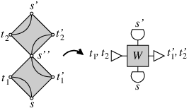
Figure 5: Graphical representation of the basic tile in the Sirker-decomposition. A composition of two transfer matrices can be depicted as a tile with four arms at the edges. The shape of the arms symbolizes the symmetries of the tile and the basis of the underlying tensor operator. The left row-to-row tile and the left corner tile arise by summing out the left free sites of . For the right row-to-row tile and the right corner tile the right free sites of are bent into the horizontal edges in order to aim a summation with the neighboring site on the lower/upper tile when composing tiles. In figure 6, the construction of all initial tiles is depicted. These initial tiles demand the construction of the initial basis. Starting from the one-site basis , the vertical basis of corner and column-to-column tile is22 2 denotes the usual tensor product. , while the horizontal basis of left corner and row-to-row tile is , and the horizontal basis of right corner and row-to-row tile is in the first iteration.

Figure 6: Graphical representation of the initial tiles. - 2.
Calculation of expectation values
All tiles are combined to form a periodically closed two-dimensional lattice in order to determine the partition function of the system. Summing out the states on the inner edges, we obtain the desired partition sum of the system. The partition sum of the modified system with a certain operator situated in the middle of the lattice (see figure 7) can be realized similarly. Thus, the thermodynamical expectation value can be computed.

Figure 7: (a) Calculation of the partition function and (b) of the partition function of the system containing a certain operator . - 3.
Enlargement of system tiles
In the next step of the renormalization process, the system is expanded by enlargement of the corner tiles in applying a row-to-row, a column-to-column tile and the basic tile. Correspondingly, the row-to-row and column-to-column tiles have to be expanded by addition of the basic tile. These enlargement steps, which technically correspond to matrix-matrix-multiplications, are illustrated in figure 8. Enlargement of the tiles implies enlargement of the bases, which is done by simple tensor products , and . Note that the sizes of the bases grow by a factor of to depending on the underlying spin system, which correspondingly increases the size of the tiles.

Figure 8: Enlargement of system tiles. (a) The enlarged corner tile is composed of the corner tile , the column-to-column tile , the row-to-row tile and the basic tile . (b) The enlarged the column-to-column tile is composed of the column-to-column tile and the basic tile . - 4.
Construction of reduced density matrices
The crucial step in the DMRG-like renormalization procedure is the construction of the reduced density matrix. In the Trotter decomposed lattice, three density matrices , and are required in order to renormalize the three different types of bases appearing in the system (see figure 9). The concept of the reduced density matrix is to compose the corner matrices and to sum out all but one edge. The picture of the reduced density matrices then corresponds to cuts of the system [15, 18]

Figure 9: Construction of the (a) vertical and (b) left reduced density matrix. Illustration as “cuts of the system”. - 5.
Truncation of basis
The idea behind renormalization group procedures is to iteratively integrate out insignificant degrees of freedom. In the context of DMRG-type algorithms, measuring the contribution of states for calculating the partition function is carried out by diagonalization of the reduced density matrix. Those eigenstates with large eigenvalues will dominate because the partition function is nothing but the trace over the reduced density matrix. Conservation of the bases’ sizes demands truncation of the eigenstates with lowest weight. So, we establish a projection onto the states with largest eigenvalues as renormalization prescription. Since a projection is obtained for each of the three bases, all edges of the system tiles are now reduced to a fixed size keeping only the most relevant states for calculation of the partition function.
- 6.
Iteration
Go to step (2) until desired system size is reached.
2.4 Normalization of growing tiles
While our interest lies in the calculation of (local) expectation values of a certain quantum mechanical system, we have to deal with the partition functions of an iteratively increased classical system in the QCTMRG-algorithm. Thus, the partition function is a rapidly growing entity leading to several huge matrix entries in the tiles’ numerical representation in each renormalization step. So, the program runs the risk of exceeding the numerical capacity of the variables of the system. To avoid this problem, a constant prefactor is extracted in each renormalization step.
2.5 Implementation
Our implementation of the QCTMRG method follows the algorithm presented in section 2.3. The ratio is kept at a fixed value during the renormalization procedure as in TMRG. This provides, in contrast to TMRG, not only a new (lower) temperature but also a different (larger) chain length after each renormalization step. Measurements of expectation values can be made in the center of odd chains or at the two sites in the center of even chains. Our implementation makes use of good quantum numbers which drastically reduce computational effort.
3 Results
As a first test, we compute the energy and the free energy of the Ising model [19]. The antiferromagnetic Ising chain with the classical Hamiltonian
| (15) |
is exactly solvable by a transfer matrix method [20]. The classical Ising spin can take the values .


We have computed the thermodynamics of the Ising chain using the QCTMRG algorithm, keeping states within the renormalization procedure. The inverse factor of temperature and number of imaginary time steps has been chosen as . We expect an excellent agreement with the analytical results because the Trotter decomposition becomes exact for the classical Ising model. In figures 10 and 11 the numerical results are plotted and, indeed, both data show the expected agreement.
We face a different situation in considering the antiferromagnetic spin- Heisenberg chain
| (16) |
The model is exactly solvable [21] but quantum fluctuations are no longer suppressed. Thus, the Heisenberg chain can serve as a non-trivial trial system for the QCTMRG algorithm.

We calculated the free energy and the expectation value of the energy operator in the middle of the chain, see Figs. 12, 14. The calculations have been done with fixed ratio while the preserved number of states from the renormalization was varied from to .
In figure 12, the free energy density is plotted against temperature. Note that the chain length is related to temperature by . With increasing the free energy tends to converge. Interestingly, the convergence is faster for lower values of and correspondingly larger system sizes. We account for that point later in Section 4.2. For a comparison, we added the well-converged data for an infinite chain calculated by conventional TMRG. We see the deviation of the QCTMRG data from this curve more pronounced at higher temperatures which are related to smaller system sizes. Thus, we can interpret the deviation as finite size effect.

For three points of fixed temperature and chain length the free energy density was extrapolated, see figure 13. We find growing with for each point. This results from the fact that the partition sum is underestimated for smaller number of states kept. This leads to a monotonically increasing free energy for growing . As already noticed earlier, we find better convergence for smaller temperature and larger system sizes.


The energy expectation value in the center of the chain has been calculated for various system sizes and temperatures in figure 14. Again we have which leads to a fixed relation for the QCTMRG data. Odd and even chain lengths are included in this calculation, in contrast to the free energy data which have only been given for even chains. For odd chains, the expectation value was taken from a plaquette at the exact center of the decomposition. For even chains, we considered one of the two central plaquettes. Even chain lengths appear as the natural choice in the renormalization procedure. Chains with an odd number of sites have a well-defined central site which might give better results.
We find the energy expectation value to lie for even systems below and for odd systems above the infinite-system value. The low-energy spectrum of the antiferromagnetic Heisenberg chain involves spin-1/2 spinons which can be identified with quantum domain walls. The ground state is a total spin singlet on chains with an even number of spins. In odd chains there is no spin singlet ground state and so always a spinon “excitation” is present. In the domain wall picture, there is always a kink present. For this reason, we expect the chains with an even number of sites to possess a lower local energy than chains with an odd number of sites. However, we expect that the expectation values for even and odd chains converge to the same limit in an infinite chain. This description agrees well with our observed behaviour.
In either case, we have a strong dependence of the expectation value on the number of preserved states in the renormalization group. For both even and odd number of sites, we can still distinguish the data curves up to low temperatures even for high values of . Yet, the convergence for even system sizes is faster than for odd sizes.
To get a more quantitative picture we plotted the convergence of several points of fixed temperature and system size, see figure 15. Like in the free energy data, the high- and larger sized systems show a better convergence. We included linear fits for a better understanding. The expectation values for even/odd sized system at finite temperatures seem to differ even in an extrapolation. The infinite-chain expectation value lies well-between those boundaries. For larger system sizes and lower temperatures we obtain a better convergence in .
The results from this section shall serve as an illustrating background for a discussion of the scope of application and the limits of the QCTMRG technique.
4 Discussion of the QCTMRG method
A crucial attribute for the QCTMRG algorithm is the fixed relation between system size and temperature during the renormalization loops. This condition sets the focus of the method to finite size systems, in contrast to the TMRG. Yet, a significant advantage in computational resources would make the QCTMRG an interesting choice for low-temperature studies of very large systems where finite-size effects play a marginal role.
4.1 Running time and storage use
For a view on the algorithm’s running time and storage use, we studied the scaling behaviour with the number of states kept of the different steps in the algorithm. We find the algorithm to take asymptotically elementary floating point operations (FLOP) and a storage use of order floating point numbers for large . However, most of the time is spent in matrix-matrix-multiplications operations where a naive approach would give a running time of FLOP for multiplication of two matrices. In contrast to this, the fastest algorithm currently known has an asymptotic running-time of FLOP [23]. So we expect the running-time to scale asymptotically with well-below fourth order in in a clever implementation.
In case of the TMRG algorithm, the by-far most time consuming part is finding the largest eigenvalues of the transfer-matrix. We, thus, expect the asymptotic scaling behaviour to be dominated by the employed Arnoldi method which performs with between and the cost of a certain matrix-vector product when is the size of the matrix. In our case, the necessary matrix-vector product has a cost of FLOP and the total matrix has a basis of size . We thus expect the total running-time to vary between worst case and best case. Further reduction might be achieved when clever algorithms for matrix multiplications are implemented. The storage scales with the size of the system-block-transfer-matrix ( numbers).
From the theoretical point of view, the QCTMRG and the TMRG algorithms have similar running-times in the large- limit. The TMRG algorithm will be favorable in those cases where the Arnoldi method reaches a fast convergence. For some ill-posed problems, however, the QCTMRG algorithm might have an advantage. The TMRG algorithm is the clear winner when storage usage is a sensible quantity.
In our implementation of both methods, we observed a roughly similar running time of both algorithms for different number of preserved states . The storage use was, indeed, higher in the QCTMRG algorithm.
4.2 Fundamental challenges
Yet, we still face some fundamental challenges of the QCTMRG algorithm in addition to the advantages of TMRG concerning the use of system resources. As already mentioned above, the quantum character of the system enforces periodical boundary conditions in Trotter direction which makes the two-dimensional corner transfer-matrix from Nishino’s CTMRG a three-dimensional tensor in the case of QCTMRG. This is the reason behind an increase in running-time and storage which is crucial and partly destroys the advantages from the development of CTMRG over TMRG.
Another more subtle point involves the spectra of the reduced density matrices from the renormalization procedure. Consider the limit which is close to the starting point of TMRG and QCTMRG where is small. Here, the local transfer-matrix of the Trotter decomposition reduces to
| (17) |
which means that the initial spin configuration will not be changed by the transfer-matrix.
Now, we consider a Trotter decomposition for infinite temperature or vanishing . The chosen graphical representation depicts the Kronecker symbols as lines passing through the transfer-matrix plaquettes. If the system is periodically closed in Trotter direction and has open boundaries in space direction, we can imagine the paths as non-interacting lines around a cylinder. This depicts the trace from the partition sum.
Building a reduced density matrix introduces a vertical or horizontal cut into the system. Consider the case of a cut in Trotter direction which corresponds to the cut in TMRG. One “spin path” has been cut through while all the others stay intact, i.e. they still are summed out in the reduced density matrix. Only the intersected thread determines the eigenspectrum of the reduced density matrix. With a straightforward calculation we find one or two degenerate eigenvalues depending on whether we intersect an odd or even number of sites. All other eigenvalues remain zero in this case. This turns the renormalization step, which is a truncation of basis states, to be highly effective. In a system with small we still find a small number of dominating eigenvalues which lead a DMRG renormalization to success.
The opposite situation is faced when the cut is made in space direction. If the underlying spin chain has spins, the density matrix will “cut” as much as paths. All spins act separately and, thus, all spin configurations have the same contribution to the partition function. Merely the remaining degrees of freedom will be summed out. Consequently, we are left with a reduced density matrix which has degenerate eigenstates when is the spin size. No effective truncation can be found. The situation in cases with high, but finite temperature is certainly less ill-posed. Though, still we expect a slow decay of the spectrum of the reduced transfer matrix.
This scenario explains why the calculated QCTMRG data shows a most significant deviation from the expected values at higher temperatures. Starting with a small system size the algorithm can still handle the system with high precision. For larger system sizes, a truncation has to be done during the renormalization step which cannot be optimal since the reduced density matrix will still have a flat spectrum. At even larger system sizes and lower temperatures the spectrum of horizontal density matrix will become acceptably well-behaved again.
5 Conclusions and Outlook
We developed a new method for finite-temperature studies of one-dimensional quantum systems based on the CTMRG of Nishino. The free energy densities and thermal energy expectation values at the chain centers have been successfully calculated for the classical Ising chain and the antiferromagnetic spin- Heisenberg chain by the Quantum Corner-Transfer Matrix DMRG. Reliable results were given for finite temperatures and system sizes. Yet, the algorithm faces two difficulties:
- •
Periodic boundary conditions reduce the efficiency.
- •
The reduced density matrix in space direction has a slowly decaying eigenspectrum.
If finite-temperature data in the thermodynamic limit are aimed at, the quantum TMRG method is certainly still the method of choice. At least one of the mentioned problems should be solved to make the QCTMRG technique an attractive option.
Acknowledgments
We dedicate this paper to Dietrich Stauffer on the occasion of his retirement. This work has been performed within the research program SFB 608 of the Deutsche Forschungsgemeinschaft.
References
- [1] S.R. White, Phys. Rev. Lett. 69, 2863 (1992).
- [2] S.R. White, Phys. Rev. B 48, 10345 (1993).
- [3] S. Östlund and S. Rommer, Phys. Rev. Lett. 75, 3537 (1995).
- [4] F. Verstraete, J.J. Garcia-Ripoll, and J.I. Cirac, Phys. Rev. Lett. 93, 207204 (2004).
- [5] I. Peschel, W. Wang, M. Kaulke, and K. Hallberg (Eds.), Density Matrix Renormalisation. A New Numerical Method in Physics, Lecture Notes in Physics 528 (Springer, Berlin, 1998).
- [6] U. Schollwöck, Rev. Mod. Phys. 77, 259 (2005).
- [7] H.F. Trotter, Proc. Am. Math. Soc. 10, 545 (1959).
- [8] M. Suzuki, Prog. Theor. Phys. 56, 1454 (1976).
- [9] M. Suzuki, Phys. Rev. B 31, 2957 (1985).
- [10] M. Suzuki, J. Math. Phys. 26, 601 (1985).
- [11] M. Suzuki, J. Stat. Phys. 43, 883 (1986).
- [12] R.J. Bursill, T. Xiang, and G.A. Gehring, J. Phys.: Condens. Matter 8, L583 (1996).
- [13] X. Wang and T. Xiang, Phys. Rev. B 56, 5061 (1997).
- [14] N. Shibata, J. Phys. Soc. Jpn. 66, 2221 (1997).
- [15] T. Nishino and K. Okunishi, J. Phys. Soc. Jpn. 65, 891 (1996).
- [16] J. Sirker and A. Klümper, Europhys. Lett. 60, 262 (2002).
- [17] J. Sirker, Ph.D. thesis, Universität Dortmund (2002).
- [18] T. Nishino and K. Okunishi, J. Phys. Soc. Jpn. 66, 3040 (1997).
- [19] E. Ising, Z. Phys. 31, 253 (1925).
- [20] H.A. Kramers and G.H. Wannier, Phys. Rev. 60, 252 (1941).
- [21] H. Bethe. Z. Phys. 71, 205 (1931).
- [22] A. Klümper and D. C. Johnston, Phys. Rev. Lett. 84, 4701 (2000).
- [23] D. Coppersmith and S. Winograd, J. Symb. Comput. 9, 251 (1990).