Keywords: stochastic particle dynamics (theory), stochastic processes (theory), models for evolution (theory)
Statistics of the total number of collisions and the ordering time in a freely expanding hard-point gas
Abstract
We consider a Jepsen gas of hard-point particles undergoing free expansion on a line, starting from random initial positions of the particles having random initial velocities. The particles undergo binary elastic collisions upon contact and move freely in-between collisions. After a certain ordering time , the system reaches a “fan” state where all the velocities are completely ordered from left to right in an increasing fashion and there is no further collision. We compute analytically the distributions of (i) the total number of collisions and (ii) the ordering time . We show that several features of these distributions are universal.
1 Introduction
Exactly solvable models of interacting particle systems are important both in equilibrium and out-of-equilibrium statistical mechanics. Such solvable models, apart from their pedagogical virtues, also offer important insights and intuitions of the underlying more complex physical phenomena. Besides, they also allow to understand better the limitations of the approximate methods one generally uses in treating many-particles systems (e.g., the Boltzmann equation).
One such very useful and instructive model was introduced a few decades ago [1, 2] and is usually referred to as the Jepsen gas [3]. It consists of identical hard-point particles that undergo binary elastic collisions on a line. At these instantaneous collisions the particles exchange their velocities, while in-between collisions they move freely. Due to the simplicity of the dynamics, this system admits analytical treatments for various imposed conditions, and therefore triggered quite a lot of interest in the past. The work of Jepsen [3] was followed by Lebowitz et al. [4, 5, 6], McKean [7], and Keyes [8] who refined and extended the calculations of the stochastic properties of a ‘test’ gas particle, including its asymptotic diffusive-like behavior and a comparison with the results of the Boltzmann equation approach. There was a recent surge of interest in this model in the context of the “adiabatic piston problem” [9, 10, 11, 12, 13], including the description of the stochastic dynamics of the piston-particle [14] and the analytic calculation of the energy transfer and heat flux throughout an inhomogeneously-prepared, out-of-equilibrium configuration of the gas [15]. Later on, the Jarzynski theorem [16] was illustrated for the case of uniform expansion or compression of the gas [17]. Jepsen gas also turned out to be useful in the study of spin transport processes in the nonlinear -model [18, 19].
In the context of biological evolution, a simplified version of Eigen’s
quasispecies model [20], namely, the shell
model [21, 22, 23] corresponds to the free expansion of
a Jepsen gas of particles, where initially there is one particle at
each position for with a positive velocity
drawn independently from a position dependent probability density function
(pdf) . A further simplification treating the velocities as
independent and identically distributed (i.i.d.) random variables with a
common independent pdf (i.e., ) leads to
the i.i.d. shell model, for which several asymptotic properties can be
computed exactly [24, 25]. In particular, the statistical
properties of the piston-particle (the rightmost particle or the leading
genotype in the biological language) exhibit universal
properties. Its velocity distribution function at intermediate times
(, where is related to the tail of the
velocity distribution) has universal scaling behavior of only three
varieties, depending exclusively on the tail of
[25]. The associated scaling functions are different
from the usual extreme-value distribution of uncorrelated random variables,
and this difference is due to the dynamically-built, collision-generated
correlations between the particles at finite times. These correlations are
also responsible for the fact that the statistics of the piston collisions
is not Poissonian. Indeed, both the mean and the variance of the number of
collisions the piston-particle undergoes increase logarithmically with
time, but with different prefactors (that are also universal).
Despite this rather rich history of the Jepsen gas, there are other interesting natural questions to which detailed answers are missing. Consider, for example, the fact that the dynamics of the freely expanding Jepsen gas provides a “natural” sorting algorithm for the velocities of the particles. It leads to an asymptotic “fan” state (see figure 1) in which these velocities are completely ordered from left to right in an increasing fashion. Two questions arise naturally from this ordering of the Jepsen gas are
- A.
What is the total number of collisions the particles undergo?
- B.
How long does it take for the gas to reach the “fan” state?
In this paper we provide analytical answers to these two questions.

More precisely, we consider the free expansion of a Jepsen gas of hard-point particles of equal mass on the infinite real line . The initial positions of the particles are drawn independently from a common pdf and a random velocity drawn independently from a common pdf is assigned to each particle. At subsequent times () each particle moves ballistically according to its assigned velocity, and upon contact between two particles they undergo elastic collision which merely interchanges their respective velocities. We assume both the set of positions and the set of velocities are continuous variables (or at least one set), so that the collisions are always binary, and there can be at most one binary collision at one instant of time. Clearly, in each collision the velocities of the colliding particles get ordered such that after the collision the particle on the right acquires the larger of the two velocities and the one on the left gets the smaller of the two velocities. Therefore, after a certain ordering time the system reaches a “fan” state where the velocities of the particles are increasingly ordered from left to right. Once this “fan” state is reached, evidently, there cannot be any further collision. For any given initial realization of positions and velocities, the dynamics of future evolution of the gas is completely deterministic. Therefore, both the total number of collisions (denoted by ) and the ordering time (denoted by ) are solely determined by the initial condition. Hence, and are random variables in the sense that they differ from one realization of initial condition to another. In this paper we analytically compute their distributions. Our main results are:
- A.
The probability of having collision, is completely independent of and for all , and for large it approaches a Gaussian form around its mean with a variance .
- B.
When the ordering time is suitably scaled with as , —where is a nonuniversal scale factor which depends explicitly on and as given by (16),— the limiting pdf of in the scaling limit , while keeping fixed, becomes universal, i.e., completely independent of and , and is given by the well known Fréchet form that arises in the extreme value statistics.
The paper is organized as follows. In section 2, we compute the statistics of the total number of collisions, and in section 3, we compute the limiting distribution of the ordering time. Section 4 contains some concluding remarks. Most of the calculational details are relegated to the Appendices A–C.
2 Total number of collisions
In order to express the total number of collisions in terms of the initial condition, we label the particles as from left to right, i.e., is the leftmost particle and is the rightmost one (see figure 1). Let for each denote the initial position of the -th particle such that . Note that the labeled, ordered coordinates ’s are no longer distributed independently according to , rather their joint pdf is given by
| (1) |
where is the Heaviside step function. On the other hand, the initial velocities associated with the labeled particles, which we denote by for are i.i.d. random variables drawn from the common pdf .
Now, for a given initial configuration, the system is fully and uniquely described at all subsequent times by the set of the free trajectories (see figure 1(a)). Note that the -th free trajectory should not be confused with the actual trajectory of the -th particle. Indeed, each of the particles travels along such a free trajectory until it collides with another particle; in such a binary collision the particles interchange their trajectories (see figure 1(b)). In terms of the free trajectories, the total number of collisions is just the total number of intersections among the free trajectories. Two free trajectories can, of course, intersect at most once.
Consider first two extreme situations. If in the initial configuration the velocities are already in the increasing order, i.e., (which happens with probability ), then there cannot be any collision at subsequent times as the gas evolves. Thus, in this case, the system is always in the “fan” state and . On the other hand, if the initial velocities are in the decreasing order, i.e., (which also happens with probability ), then each pair of free trajectories intersects once and there are of them. Therefore, this configuration yields the maximum number of binary collisions, which is . For any other realizations of the velocities, lies between and . The total number of collisions is a random variable, , which differs from one realization of the initial configuration of the particle velocities to another, and whose statistical properties we address below.
Since, for , two free trajectories and intersect if and only if for . Therefore, for a given realization of the initial velocities , the total number of collisions (total number of intersections among free trajectories) can be expressed as
| (2) |
Obviously, is independent of the set of initial positions of the particles and their distribution. Moreover, we will show below that is also completely independent of the velocity distribution and is solely determined by .
The probability of having total number of collisions can be formally expressed as
| (3) |
where with integer , is discrete delta function: and for any . Let us consider the change of variables [26]
| (4) |
Obviously is a monotonically increasing function of , and therefore . Moreover, since is normalized to unity, the variables vary from 0 to 1, and so (3) becomes
| (5) |
where the velocity distribution simply drops out, meaning that is universal, i.e., is the same as if the “new” velocities are drawn independently from an uniform distribution over .
The mean number of total collisions is straightforward to compute. Using the change of variables in (4), it is trivially checked that . Therefore, taking the average in (2) yields
| (6) |
The calculation of the variance implies several steps that are indicated in A. One obtains finally:
| (7) |
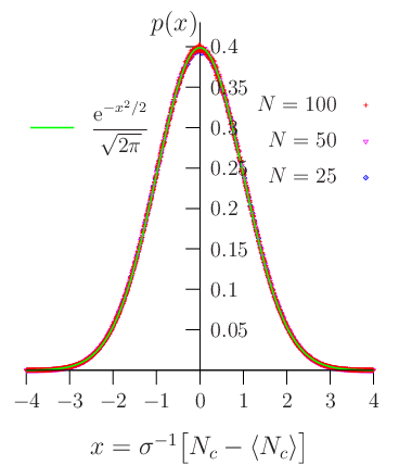
As given by (2), is a sum of random variables that are correlated. However, each term in (2) is correlated with only other terms, since two different terms are correlated only when they have one velocity in common. Therefore, near the mean and within a region , the probability distribution for large has a Gaussian form (see B),
| (8) |
One can check numerically that this is actually already an extremely good approximation for as small as and for practically all the values of , as illustrated by the figure 2.
3 Ordering time

In order to compute the statistics of the ordering time , it is convenient to relabel the particles according to the decreasing order of the velocities (see figure 3). Let denote the decreasingly ordered set of the initial velocities, i.e.,
so that . The joint pdf of these ordered velocities is given by
| (9) |
Let for each denote the initial position of the particle having the initial velocity . Note that when we label the particles according to the order of their velocities, their initial positions ’s are no longer ordered on the line, but are i.i.d. random variables drawn from the pdf .
As before, for a given initial condition, the system is fully and uniquely described at all subsequent times by the set of free trajectories , where . The “fan” state is reached when all the free trajectories become completely ordered according to the velocities, i.e., at all (see figure 3).
Let be the cumulative probability distribution of the ordering time, i.e., . It immediately follows that , given that . This probability can be formally expressed as
| (10) |
where denotes the averaging over both the i.i.d. initial positions that are drawn from the common pdf , and the initial ordered velocities, whose joint pdf is given by (9). Note that, for any finite is non-zero,
| (11) |
and is universal. This represents the probability that the initial positions of the particles are also ordered according to their velocities, i.e., , so that there cannot be any collision. The pdf of the ordering time is simply
| (12) |
where the extra weight at vanishes in the limit .
Let us introduce the variables and for brevity. In terms these variables we rewrite the expression (10) as
| (13) |
where for .
Since ’s are drawn independently from , two different variables and with are correlated iff . Therefore, for large , treating ’s as i.i.d. random variables, with a common pdf , is a rather good approximation, which becomes exact in the limit . On the other hand, in the variables (), the ordered velocities are correlated, as can be seen from their joint pdf given by (9). Therefore, the random variables with , are not independent either. It turns out, however, that the limiting distribution of the ordering time , when suitably scaled with , has the well known Fréchet form (see figure 4) that arises in the extreme value statistics of i.i.d. random variables drawn from a common parent distribution with a power-law tail. To show this, we formally expand the product in (13) as a sum of terms
| (14) | |||||
We show in C that scales as when both and are large. Moreover, as detailed in C, considering first , and then taking the scaling limit and , but keeping fixed, the -th term (counting from the “zero”-th term, which equals unity) in (14) becomes
| (15) |
where
| (16) |
with, recall,
| (17) |
Thus, (14) yields
| (18) |
The limiting pdf of the scaled ordering time , —where the scale factor is nonuniversal and is given explicitly by (16),— is therefore given by the universal function . Figure 4 compares the results of the numerical simulation of the gas with this limiting pdf.

The Fréchet cumulative distribution (18) usually emerges as the cumulative distribution of the maximum of a set of i.i.d. random variables each drawn from the common pdf having a power-law tail . In the context of Jepsen gas, let us consider two free trajectories and chosen at random. The ordering time between these two free trajectories has the pdf
| (19) |
where is given by (16). The ordering time of the full system is clearly the maximum of the ordering times between each of the ( for large ) pairs of free trajectories. Therefore, it turns out simply that in the , the ordering times between different pairs of free trajectories become uncorrelated, and can be treated as i.i.d. random variables drawn from a common pdf having power-law tail .
4 Concluding remarks
In this paper we have computed the statistics of the total number of collisions of a freely expanding gas of hard-point particles, and found that the mean is . On the other hand, the variance is , due to the correlations between different particle collisions, without which the variance would also have been . However, despite these correlations, the probability distribution of the total number of collisions near the mean is very well approximated by a Gaussian form.
In the context of biological evolution of quasispecies, the evolution time —which is defined as the time at which the rightmost particle undergoes the last collision, i.e., the free trajectory with the largest slope (with respect to the time-axis) becomes the rightmost trajectory— was studied recently [21, 27]. It was estimated that its pdf has a power-law tail . The ordering time studied here represents obviously the upper bound to this evolution time, . We have found that the limiting distribution of the ordering time, when suitably scaled with , becomes universal and is given by the Fréchet form. This Fréchet form usually appears as the limiting distribution of maximum of a set of i.i.d. random variables drawn from a common distribution with a power-law tail. Our result here provides another mechanism of generating Fréchet form as a limiting distribution.
Finally, while we have studied the statistics of the total number of collisions, it would be interesting to study the number of collisions of the particles up to time . Our results correspond to the limit . In this context we point out that recently the collision statistics of a tagged particle in a -dimensional hard-sphere gas at equilibrium was investigated using Boltzmann equation approach [28] and was found to be non-Poissonian. It would be interesting to verify this conclusion for a tagged particle in the 1- Jepsen gas for which an exact result may be possible to obtain.
Appendix A Variance of the total number of collisions
Subtracting the mean given by (6) from (2), then taking the square and the average gives
| (20) |
where
| (21) |
Note that, , and .
The total number of terms in the summation in (20) is . These can be grouped according to the correlation functions ’s that are of similar kind. This can be conveniently represented by diagrams as shown in Fig. 5. Then using the change of variables (4), it is easy to compute the correlations and hence , corresponding to each of the diagrams (a)–(f) in figure 5.

- Diagram (a):
-
.
The number of such terms in (20) is equal to number of ways of choosing two indices out of , which is
- Diagram (b):
-
.
The number of such terms in (20) is equal to number of ways of choosing three indices out of with allowing permutation between two of them . This is given by
- Diagram (c):
-
Same as for diagram (b).
- Diagram (d):
-
.
The number of such terms in (20) is just the number of ways of choosing three indices out of , which is
- Diagram (e):
-
Same as for diagram (d).
- Diagram (f):
-
. These terms do not contribute to the sum in (20).
Therefore, finally (20) yields
| (22) |
Appendix B Probability distribution of the total number of collisions
Let us consider the deviation of the total number of collisions given by (2) from it mean given by (6):
| (23) |
where , and . Obviously and we have already calculated the second moment in A, which is
| (24) |
Assuming the pdf of the velocities to be symmetric, i.e. , and noting that , it can be easily shown that the probability distribution of is symmetric about zero. On the other hand, we have shown in section 2, that the probability distribution of , and hence that of , is independent of the velocity distribution. Therefore, the distribution of must be symmetric for any velocity distribution. This implies the vanishing of all the odd moments, i.e.,
| (25) |
By the same argument, one can also show that average over any product of odd number of ’s is zero. is just a sum of such terms.
The even moments are given by
| (26) |
for . We first break the average as product of averages over different factors of pair of ’s, and then sum over the indices independently under each average of factors, each of which gives the second moment making it . This is . The corrections to this come from the terms where the sets of indices between different factors are not independent. If there is one common index between two different factors, we will have to take the average of them together. It will reduces one summation and therefore is . The number of ways of grouping objects into pairs is clearly . Therefore,
| (27) |
Let us now consider the scaled variable
| (28) |
Since is , we have
| (29) |
The characteristic function of the probability density of is then
| (30) | |||||
The inversion of this Fourier transform gives the pdf of as
| (31) |
which says that the scaled variable has a Gaussian distribution.
Appendix C Evaluation of the terms in the series expansion of
First term:
Let us compute the average , in the first term (counting from the “zero”-th term, which equals unity) in (14). The pdf of is given by
| (32) | |||||
in which
| (33) |
The integrand in (32) merely specifies that velocities are smaller than , velocities are larger than , two velocities are and respectively, such that their difference is . The combinatorial prefactor gives the number of such arrangements, and we finally integrate the integrand over all possible values of . It is checked that this pdf is normalized, . Using (32) we first take the average over , which for all gives
| (34) | |||||
When ,
| (35) |
Note that the pdf of as given by (17) is independent of the index . Substituting (35) in (34), then taking average over , and finally summing over yields
| (36) |
with given by the (16).
Second term:
Let us now consider the second term in (14) involving summation over and . We substitute , and rewrite it as
| (38) | |||
| (39) |
Now in the first term (38), the variables and are uncorrelated, and each of them has the same pdf (17). Following the similar reasoning that we used to write down the pdf of the single variable in (32), we can also write down the joint pdf of and for as
| (40) | |||||
where is given by (33). It is checked that the joint pdf is normalized to unity, i.e., . Now using (40) we first compute the average over and in (38), then we expand the result in Taylor series (assuming large ), and then average over and . Finally, we sum over and , and take the limit . Noting that
| (41) |
we find
| (42) |
where is given by (16). The term (39) goes to zero in the limit .
The -th term:
Following the exactly same steps, we can evaluate the -th term of the expansion of in the expression (14). We first assume that , and later take the limit . We again write the sum as
| (43) | |||
| (44) |
such that (43) contains only the terms with for all . As before, the variables in (43) are uncorrelated, and the joint pdf of can be written as
| (45) | |||||
where is given by (33) and where the combinatorial prefactor gives the number of ways of arranging velocities as in the above integrand,
| (46) |
It is again checked that the joint pdf (45) is normalized, i.e.,
| (47) |
Using (45) we first take the average over in (43), then we expand the result in Taylor series (assuming large ), and then average over . Finally, summing over all the indices , and taking the limit , (43) yields
| (48) | |||||
| (49) |
Now, the term inside the first square brackets of the integrand in (49) remains unchanged under permutations of the variables . While the term inside the second square brackets of the integrand changes under permutations, summing over all possible permutations yields unity. However, note that ’s are just dummy variables in the multiple integral (49), so it must remain unchanged under any of the permutations of these variables. Therefore, the integral (49) equals
| (50) |
Therefore, in the limit the expression (43) becomes [see (48), (49)],
| (51) |
where is given by (16). The remaining term (44) goes to zero in the limit .
References
References
- [1] Frisch H L 1956 Poincaré Recurrences Phys. Rev. 104 1
- [2] Teramoto E and Suzuki C 1955 The Statistical Mechanical Aspect of H-Theorem Prog. Theor. Phys. 14 411
- [3] Jepsen D W 1965 Dynamics of a Simple Many-Body System of Hard Rods J. Math. Phys. 6 405
- [4] Lebowitz J L and Percus J K 1967 Kinetic Equations and Density Expansions: Exactly Solvable One-Dimensional System Phys. Rev. 155 122
- [5] Lebowitz J L, Percus J K and Sykes J 1968 Time Evolution of the Total Distribution Function of a One-Dimensional System of Hard Rods Phys. Rev. E 171 224
- [6] Aizenman M, Lebowitz J L and Marro J 1978 Time-displaced correlation functions in an infinite one-dimensional mixture of hard rods with different diameters J. Stat. Phys. 18 179
- [7] McKean H P 1967 Chapman-Enskog-Hilbert expansion for a class of solutions of the telegraph equation J. Math. Phys. 8 547
- [8] Protopopescu V and Keyes T 1985 The Goldstein-McKean model revisited Physica A 132 421
- [9] Lieb E 1999 Some problems in statistical mechanics that I would like to see solved Physica A 263 491
- [10] For a critical discussion of the “adiabatic piston problem” see Gruber Ch 1999 Thermodynamics of systems with internal adiabatic constraints: Time evolution of the adiabatic piston Eur. J. Phys. 20 259
- [11] Piasecki J and Gruber Ch 1999 From the adiabatic piston to macroscopic motion induced by fluctuations Physica A 265 463
- [12] Piasecki J and Sinai Ya G 2000 A model of non-equilibrium statistical mechanics in Dynamics: Models and Kinetic Methods for Non-equilibrium Many Body Systems Karkheck J (ed) (Amsterdam: Kluwer Academic) pp 191-199
- [13] Piasecki J 2001 Drift Velocity Induced by Collisions J. Stat. Phys. 104 1145
- [14] Balakrishnan V, Bena I and Van den Broeck C 2002 Velocity correlations, diffusion, and stochasticity in a one-dimensional system Phys. Rev. E 65 031102
- [15] Balakrishnan V and Van den Broeck C 2005 Analytic calculation of energy transfer and heat flux in a one-dimensional system Phys. Rev. E 72 046141
- [16] Jarzynski C 1997 Nonequilibrium Equality for Free Energy Differences Phys. Rev. Lett. 78 2690
- [17] Bena I, Van den Broeck C and Kawai R 2005 Jarzynski equality for the Jepsen gas Europhys. Lett. 71 879
- [18] Sachdev S and Damle K 1997 Low Temperature Spin Diffusion in the One-Dimensional Quantum Nonlinear Model Phys. Rev. Lett. 78 943
- [19] Sachdev S and Young A P 1997 Low Temperature Relaxational Dynamics of the Ising Chain in a Transverse Field Phys. Rev. Lett. 78 2220
- [20] Eigen M 1971 Selforganization of matter and the evolution of biological macromolecules Naturwissenschaften 58 465
- [21] Krug J and Karl C 2003 Punctuated evolution for the quasispecies model Physica A 318 137
- [22] Jain K and Krug J 2005 Evolutionary trajectories in rugged fitness landscapes J. Stat. Mech.: Theor. Exp. P04008
- [23] Jain K 2007 Evolutionary dynamics of the most populated genotype on rugged fitness landscapes Phys. Rev. E 76 031922
- [24] Sire C, Majumdar S N and Dean D S 2006 Exact solution of a model of time-dependent evolutionary dynamics in a rugged fitness landscape J. Stat. Mech.: Theor. Exp. L07001
- [25] Bena I and Majumdar S N 2007 Universal extremal statistics in a freely expanding Jepsen gas Phys. Rev. E 75 051103
- [26] Majumdar S N and Martin O C 2006 Statistics of the number of minima in a random energy landscape Phys. Rev. E 74 061112
- [27] Krug J 2002 Tempo and mode in quasispecies evolution in Biological Evolution and Statistical Physics Lässig M and Valleriani A (eds) (Berlin: Springer) pp 205-216 (Preprint arXiv:cond-mat/0103443)
- [28] Visco P, van Wijland F and Trizac E 2008 Collisional statistics of the hard-sphere gas Preprint arXiv:0803.1291