Negative differential resistivity in superconductors with periodic arrays of pinning sites
Abstract
We study theoretically the effects of heating on the magnetic flux moving in superconductors with a periodic array of pinning sites (PAPS). The voltage-current characteristic (VI-curve) of superconductors with a PAPS includes a region with negative differential resistivity (NDR) of S-type (i.e., S-shaped VI-curve), while the heating of the superconductor by moving flux lines produces NDR of N-type (i.e., with an N-shaped VI-curve). We analyze the instability of the uniform flux flow corresponding to different parts of the VI-curve with NDR. Especially, we focus on the appearance of the filamentary instability that corresponds to an S-type NDR, which is extremely unusual for superconductors. We argue that the simultaneous existence of NDR of both N- and S-type gives rise to the appearance of self-organized two-dimensional dynamical structures in the flux flow mode. We study the effect of the pinning site positional disorder on the NDR and show that moderate disorder does not change the predicted results, while strong disorder completely suppresses the S-type NDR.
pacs
74.25.QtI Introduction
Negative Differential Resistivity (NDR) and Conductivity (NDC) can be observed in various non-linear media. To illustrate the counterintuitive nature of this phenomenon, let us consider a force acting on a set of moving particles: NDC corresponds to a lower velocity of motion for these particles when the force applied to them increases. Two different types of NDR can be observed in the voltage-current characteristics (VI-curves) of non-linear media [1, 2, 3, 4, 5, 6, 7]. NDR of S-type is characterized by the existence of three different values of the current corresponding to a single value of the voltage . The corresponding VI-curve is S-shaped. A VI-curve with three different values of the voltage for a single value of the current is referred to as NDR of N-type. The corresponding VI-curve is N-shaped. NDR (or NDC) is commonly observed in semiconductors, plasmas, superconductors and is used in many non-linear devices (see, e.g. Refs. 1, 2, 3, 4, 5, 6, 7). In particular, semiconductors with NDR are the basic elements of Gunn-effect diodes and -junctions [1, 2]. VI-curves with NDR can only be observed under specific conditions. For example, to study N-type NDR one has to include the corresponding sample in an electric circuit with fixed voltage . Vice versa, to observe S-type NDR the sample should be included in a circuit with fixed current . If these conditions are not fulfilled, the uniform current flow becomes unstable, and non-uniform self-organized structures (e.g., filaments and overheated domains with higher or lower electric fields) arise in the sample. Such structures are commonly observed in plasmas, semiconductors, and superconductors (see, e.g. Refs. 1, 2, 3, 4, 5, 6, 7). Table 1 (using results from Refs. 1, 2, 3, 4, 5, 6, 7, 8, 9, 10, 11, 12, 13 compares NDR in different non-linear media. Note, the macroscopic manifestations of NDR in different media could be rather similar while the intrinsic physical mechanisms giving rise to NDR could be different.
| Superconductors | Semiconductors | Plasmas | Manganites | |
| Carriers | flux quanta | charge quanta: | electrons | electrons, |
| electrons or holes | holes | |||
| Characteristic | voltage-current | current-voltage | IV curve | IV curve |
| curve | (VI) curve | (IV) curve | ||
| Homogeneous | homogeneous flux | homogeneous | homogeneous | homogeneous |
| state | and current flows | current flow | current flow | current flow |
| Origin of | in/commensurate vortex | non-linear electron | ionization | |
| S-shape NDR | dynamical phases in PAPS | transport | ||
| Origin of | overheating, Cooper pair | overheating, electron | heating | heating [12, 13] |
| N-shape NDR | tunnelling [8]; vortex-core: | or hole tunnelling | ||
| shrinkage [9] (); | ||||
| expansion [10], driven [11] | ||||
| () | ||||
| Filaments | overheating, Cooper pair | current filaments, | current filaments, | |
| tunnelling [8]; vortex-core: | pinch-effect | pinch-effect | ||
| shrinkage [9] (); | ||||
| expansion [10], driven | ||||
| vortices [11] () | ||||
| Domains | vortex-induced higher | higher electric field | higher electric | higher electric |
| field overheated domains | overheated domains | field overheated | field overheated | |
| domains | domains |
As a non-linear medium with NDR, we study a superconductor with artificial pinning sites. The magnetic flux behavior in such superconductors has attracted considerable attention due to the possibility of constructing samples with enhanced pinning as well as with novel and unusual voltage-current characteristics [14, 15, 16, 17, 18, 19]. Present-day technology allows the fabrication superconductors with well-defined periodic arrays of pinning sites (PAPS). Such structures include many thousands of elements with controlled microscopic pinning parameters. Increased interest on these systems has arisen in recent years, and a number of intriguing features related to PAPS has been revealed.
In Ref. 20 the existence of several dynamical vortex phases was predicted for square PAPS subjected to perpendicular magnetic field, , close to the first matching field , where is the magnetic flux quantum and is the PAPS period. The geometry of the problem is shown in Fig. 1 which is discussed in Sec. II. The effect of the dynamic phases on the VI-curve is illustrated in Fig. 2a. Let us assume that the field is slightly higher than and the number of the vortices in the sample is higher than the number of the pinning sites . Let us now slowly increase the applied current in the sample. For very low current density (phase I in Fig. 2) all vortices are pinned and their average velocity is zero. With increasing the current , interstitial vortices, , start to move and the velocity becomes nonzero and grows with (phase II in Fig. 2). With further increasing the current , the driving force acting on a single vortex, , overcomes the pinning force, and a significant fraction of the vortices start to move. This motion is uniform and very disordered. Phase III corresponds to such vortex-flow mode. At higher vortex velocities, the random motion of vortices becomes more ordered. Some vortices become pinned in commensurate rows while others move along vortex rows, which are incommensurate with the underlying PAPS. Namely, when exceeds a threshold value, only incommensurate vortex rows move and the vortex velocity exhibits a significant drop with the increase of the driving force (phase IV). Note that the phases III and IV have an analogy with the NDR behavior of electron motion in semiconductors with the increase of the voltage. Namely, increasing the applied force on the moving particles produces a lower velocity in them. At high current densities, the driving force completely overcomes the pinning force (phase V) and the curve tends to a linear one.
The results obtained in Refs. 20 and 21 prove that the VI-curves of superconductors with a square PAPS have a part with NDR of the S-type, since the electric field in the sample is related to the average vortex velocity by the well-known relation . Such type of NDR is usual for plasmas [6, 7] and semiconductors [1, 2] giving rise to important instabilities of the uniform current flow known as pinch-effect and filamentary instability, when a current flow breaks into filaments with lower and higher current densities [1, 2, 3, 4, 5, 6, 7]. In superconductors we have only few examples of the S-type NDR in the samples with the specific weak links [10].
The described dynamical phases disappear in the case of very disordered pinning arrays and, consequently, the NDR of S-type in the VI -curves vanishes. Under realistic experimental conditions, the properties of the superconductor in the flux flow regime are strongly affected by Joule heating since the current density necessary to overcome the pinning force is high [5]. An increase of the sample temperature due to Joule heat, , gives rise to a decrease of the pinning force, and the current density can drop down with the growth of the electric field. As a result, the VI-curve with an NDR of N-type (red dashed line in Fig. 2b) is commonly observed in superconductors for high current density [4, 5]. The uniform state in samples with NDR of N-type is also unstable [1, 2]; and a propagating resistive state boundary or the formation of resistive domains can destroy the uniform flux flow mode in the superconductor [4, 5, 8]. Increasing the pinning force and/or decreasing the thermal coupling of the sample with its environment (which decreases the cooling rate of the sample), one can achieve a situation where the NDR of both N- and S-type simultaneously coexist in the VI-curve (Fig. 2b) [21]. In this case, we predict remarkable flux flow instabilities. Note also that the effect of thermal fluctuations on the flux flow regime in the superconductors with PAPS is somewhat analogous to the effect of positional disorder in the pinning sites. This effect should be taken into account, especially, at temperatures close to the critical temperature of the the superconductor .
The effect of Joule heating on the VI-curve of superconductors with PAPS was first outlined in Ref. 21. This gives rise to the coexistence of both types of instabilities, which is very unusual since non-linear devices are typically either N-type or N-type, but not both. Here we present a detailed analysis of this problem. In addition, we study in detail the effect of disorder on this phenomenon.
The paper is organized as follows. In Section II we formulate the model of the flux motion taking into account the effect of Joule heating. The heating manifests itself in thermal fluctuations of the vortices and a variation of the superconductor parameters due to the temperature increase. Both of these effects are included in the model. In Section III the average velocity of the vortices, , is found as a function of the applied current density . This dependence is obtained by means of the molecular dynamics integration of the equations of motion presented in Section II. As a result, we obtain the VI-curves of the sample with PAPS and study the effects of temperature variation, thermal fluctuations, and positional disorder of the pinning sites on these curves. In Section IV an analytical criterion for the development of the filamentary instability in superconductors with an NDR of S-type is derived. In Section V we analyze the effect of the interplay between S-type and N-type NDR on the flux flow in superconductors with a PAPS. We argue that the coexistence of the NDR of both types can give rise to macroscopic non-uniform self-organized dynamical structures in the flux flow regime.
II Model
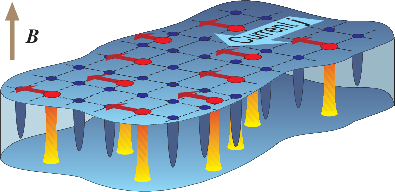
We describe the flux motion in a three-dimensional (3D) superconducting slab, infinite in the -plane, using a 2D model (assuming no changes in the -direction). This approach has also been used in the past, e.g., in Refs. 20, 21, 22, 23. We consider a sample with a square array of pinning sites interacting with vortices related to the magnetic field by . The magnetic field is perpendicular to the slab (see Fig. 1). The period of the regular array is and we focus on the case when the magnetic field is slightly higher than the first matching field , that is . The vortices are driven by the Lorentz force, , produced by the current flowing in the direction (see Fig. 1). Thus, the horizontal axis of figures 2, 3, 4, and 5, refer to the driving force or driving current , since these are proportional to each other. The overdamped motion of the th vortex is described by the equation
| (1) |
where is the velocity of th vortex, is the flux flow viscosity, is the normal conductivity, and is the upper critical field. is the force per unit length acting on the th vortex due to the interaction with other vortices. The force per unit vortex length describes the interaction of the th vortex with the pinning array. The term arises due to the thermal fluctuation contribution to the force. As in standard approaches is a random function of time , obeying the correlation relations
| (2) |
and
| (3) |
where is the Boltzmann constant, denotes a time average, is the Kronecker symbol, and delta-function.
We describe the vortex-vortex interaction by the usual expression for Abrikosov vortices
| (4) |
where is the magnetic field penetration depth, is the first order modified Bessel function, the summation is performed over the positions of vortices in the sample, and is a unit vector in the direction of the force acting between the th and th vortices.
The pinning sites (narrow indentations or “blind holes” which can accomodate a maximum of one vortex, for the vortex densities used in our calculations) are located at positions . The pinning potentials are approximated by parabolic wells. Then, the pinning force per unit length acting on the th vortex can be written in the form
| (5) |
where is the size of the elementary pinning potential well, is the maximum pinning force, is the Heaviside step function, , and is the unit vector in the direction of the elementary pinning force. In what follows, we estimate the maximum pinning force as
| (6) |
where is the coherence length.
The temperature dependence of the values entering our model is found using the Ginzburg-Landau approach. Therefore, . The temperature dependence of the penetration depth is approximated as
| (7) |
We assume that the Ginzburg-Landau ratio is independent of temperature. In this case, for the temperature dependence of the maximum pinning force, we have
| (8) |
where . We also assume that the normal conductivity is temperature independent.
We simulate Eqs. (1)–(5) using the molecular dynamics technique. Below we present the results for rectangular cells with size . Periodic boundary conditions are imposed at the cell boundaries. First, we should prepare an initial state of our system. For this purpose we assume that the initial temperature of the system is high and that the vortex structure is in a liquid unpinned state. Then, we slowly decrease the temperature down to and vortices are captured by the pinning sites. When cooling down, vortices adjust themselves to minimize their energy, simulating field-cooled experiments. Starting from this initial state, we increase the driving current and compute the average vortex velocity , which is determined as
| (9) |
where is the unit vector in the direction.
The equilibrium temperature distribution in the sample can be found by solving the heat equation with Joule heating. The average power of this heating per unit volume due to vortex motion is . The heat flux, , removed from the sample boundaries by the external coolant is described by the usual linear Kapitza law, , where is the sample surface, is the heat transfer coefficient, and the ambient temperature. To simplify the procedure, we assume that the heat conductivity of the sample, , is large, , where is the sample thickness. Under such a condition, the temperature in the sample is uniform and it can be found from the heat balance equation [5]:
| (10) |
where is the sample volume. Further, we shall assume that and neglect .
We now introduce dimensionless variables. The dimensionless current (which is equal to the dimensionless driving force ), dimensionless average vortex velocity , and dimensionless magnetic field induction , are given by
| (11) |
The normalization values and are defined by
| (12) |
In dimensionless units the heat balance equation (10) relates the temperature and the dimensionless driving force as
where
| (13) |
is the ratio of the characteristic heat release to heat removal. In our calculations we used the values of the parameters characteristic of high temperature superconductors: Å, , s-1, Å, K, G, and W/cm2K. In this case, we find that and is of the order of . In the simulations, we used and .
III Simulation results
III.1 Effect of heating: VI-curve of N- and S-type
The calculated dependence of versus the current density in the absence of the Joule heating is shown in Fig. 2a, in dimensionless units. The shape of this curve is similar to that as found in Ref. 20 and 21: there exist five dynamical vortex phases described in the introduction and a pronounced hysteresis for increasing and decreasing current regimes.
A significant effect of the heating is observed if the current density exceeds some threshold value, for the case shown in Fig. 2b. In particular, the jump from phase II to phase III becomes larger, and an abrupt transition occurs between regimes IV and V, compared to the non-heating case shown in Fig. 2a. The most important feature related to Joule heating in the high current range is the appearance of hysteresis in some regions of phases IV and V. For decreasing current, the overheated vortex lattice keeps moving as a whole at lower currents than the “cold” one (for increasing ). The transition part of the curve from phase IV to phase V is shown by the dashed line in Fig. 2b. This part of the VI-curve is unstable for a given drive force and could be only found for a fixed voltage [4].
As a result, we obtain a new complex NDR of a hybrid nature with both - and -type instabilities, which is very unusual for any media, especially for superconductors. Each type of NDR is characterized by its specific instabilities [1, 2, 3, 4, 5, 6, 7]. Thus, the obtained VI-curve is characterized by two kinds of instabilities. For example, if the current density exceeds the value (point A in Fig. 2b), the uniform current flow becomes unstable and a filamentary instability [1, 2] occurs. Due to this instability, the current flow breaks into filaments with different supercurrent density, some with lower current (state B) and others with higher current (state C). However, the state C is, in its turn, unstable and decays. The corresponding stable states are on the lower (E) and on the upper (D) VI-curve branches. That is, the filament breaks into domains with higher and lower value of vortex flow speed ; in other words, with higher and lower electric field. The stability and evolution of such a complicated structure is an open question (see also Section V).


In Fig. 3, the average vortex velocity is shown for different radii of the pinning sites. The shape of the function only slightly changes for the radii in the range to (Figs. 3a, b). However, for radii smaller than a certain value, phase IV in the reverse branch (i.e., when decreasing the driving current ) disappears (Fig. 3c) since the overheated vortex lattice cannot adjust itself to the pinning array and turns to the disordered motion in phase III.
III.2 Effect of disorder
Let us study the effects of disorder on the NDR. Small disorder can be effectively introduced to the system by increasing the radius, , of the pinning sites. So vortices acquire an additional degree of freedom and can move inside the pinning sites. The function is shown in Fig. 4 for larger pinning site radii, (Fig. 4a), and (Fig. 4b). In case of larger radii, phase III disappears, and the motion of interstitial vortices (phase II) transforms directly to the 1D incommensurate vortex motion (phase IV) (Fig. 4a). However, the robust hysteresis related to heating remains. For larger radii of the pinning sites, phase II, related to the motion of interstitial vortices, disappears since all the vortices are pinned for weak enough drives (Fig. 4b).

To model disorder related to a distortion of the regular PAPS, we introduced small random displacements for each pinning site. Specifically, for the displacement of each pinning site we consider a random angle () and a random radius (, measured in units of , where is a period of the (regular) pinning array) for each pinning displacement.

The corresponding values of are shown in Fig. 5 for different amounts of disorder. Note that small disorder does not appreciably influence (Fig. 5a). However, for (Fig. 5b), phase IV disappears in the reverse branch of . For (Fig. 5c), phase IV is lost in both branches; only some reminiscent features remain, which disappear for larger (Figs. 5d, e). Finally, at full disorder (Fig. 5f), only phases I, III and V remain. However, even in this case there is a weak hysteresis related to heating (inset to Fig. 5f), observed in experiments with random pinning [5].
IV Filamentary instability
It is well-known that the uniform current and electric field distributions are unstable under definite conditions if the sample VI-curve has parts with NDR [1, 2, 3, 4, 5, 6, 7]. Let us assume that the sample with the VI-curve shown in Fig. 2b is in a current-biased regime. If the driving current exceeds the value , the uniform current flow with the current density becomes unstable with respect to the so-called filamentary instability [1, 2]. Thus, the current flow in the sample breaks up into stripes or filaments with two different alternating current densities. This process is illustrated in Fig. 1b: the sample in state A with current density breaks into filaments with lower (state B) and higher (state C) current densities.

To study the process in more detail, we consider a sample connected to a standard electrical circuit, Fig. 6. The circuit equation is
| (14) |
where is the current in the circuit, and are the circuit inductance and resistance, is the sample length, is the electric field in the sample, is the voltage at the circuit terminals, which is assumed to be constant, and , where is the sample cross-section. Using Eq. (14) and Maxwell equations we can write the equations describing the development of the small perturbations of electromagnetic field , , and current density in the form
| (15) | |||
Here
all quantities are assumed averaged over a volume including a large number of vortices, and denote the average values over the sample cross-section. Below we assume for simplicity that the sample has zero demagnetization factor.
We shall seek the solution to Eqs. (15) in the standard form: ; where is the value to be found, and is the circuit relaxation time.
An instability develops if . In general we should add to Eqs. (15) the equation for the small temperature perturbations but here we study the filamentary instability for which the temperature rise is not of crucial importance. We also neglect the self-field effect and assume that the background magnetic field in the sample is uniform. To find the filamentary instability criterion we can consider the perturbations depending on the coordinate only [1, 2]. In such a geometry, the perturbation of the electric field has only the component, while has only the component. Using , we find from Eqs. (15)
| (16) | |||||
| (17) |
where prime means differentiation over the dimensionless coordinate , is the sample half-width, , and
are the sample VI-curve parameters, which are positive or negative depending on the relevant part of the VI-curve at given background fields and . Note that the value of is the characteristic time of the magnetic field relaxation in the sample.
The differential equation (17) requires two boundary conditions. We obtain the first one assuming that the applied magnetic field is constant. This means that or . From the Maxwell equations (15) we get . Using these ’s, and substituting from Eq. (16), we obtain the second boundary condition in the form
where
The solution of Eq. (17) reads
| (18) |
where are constants and
Substituting Eq. (18) to the boundary conditions we obtain a set of uniform linear equations for the constants . The non-trivial solution of this equation set exists if its determinant is zero. Thus we find the equation for the eigenvalue spectrum in the form
| (19) |
In the simplest case of small , when
the solution of Eq. (19) can be readily found explicitly with an accuracy up to
| (20) |
It follows from the last relation that the instability occurs only at the VI-curve branch with NDR when
and, moreover, the drop of the voltage should be large enough,
| (21) |
In this case are purely imaginary numbers and the solution of Eqs. (14) is periodic in the -direction. The characteristic spatial period of the arising current filament structure is of the order of
| (22) |
In a very unstable state, , the filament width is small, . The characteristic instability build-up time becomes . Thus, a sample with an S-type NDR in VI-curve divides itself into small filaments with different current densities (in different dynamic flux flow phases III and IV) if the resistance and inductance of the external circuit are restricted by inequalities
| (23) |
The obtained results are valid if
According to Eq. (21), the left hand side of the last inequality should be higher than unity, while the right hand side is much smaller than 1 for the parameter range studied in the previous sections if the sample half-width mm. Note, however, that taking into account the magnetic field dependence of the VI-curve gives rise to some increase in its stability.
V Interplay between N-type and S-type instabilities
In the stationary inhomogeneous state that arises after the development of the filamentary instability, the electric field should be uniform over the sample. The part, , of the filament with the higher current and the part, , with the lower current (see Fig. 2b) are defined by an evident condition , that is,
For the case shown in Fig. 1b we find an estimate .
As shown in Fig. 4, sufficiently high disorder destroys the NDR of S-type in the VI-curve, but the NDR of N-type can still exist in this case due to sample heating. Such an unstable regime has been thoroughly studied for superconductors [3, 4, 5], and we do not discuss it here.
A richer dynamics can be observed if the VI-curve has NDR parts of both N- and S-types, Figs. 2b and 3. In this case the filaments with higher current density are unstable if the system is far from the voltage-biased regime [1, 2]. The instability of the filament with N-type VI-curve should switch the filaments into state D (Fig. 2b) with high resistivity or to the formation of the domain structure with higher, D, and lower, E, resistivity [4]. However, any possible decay of the unstable state C gives rise to a non-uniform electric field distribution in the sample and, as a result, to non-zero . Thus, the state that appears after the instability develops is not stationary but rather a dynamic one.

To clarify the situation, we consider two possible VI-curves shown in Fig. 7 (one red and another, labelled by ”2”, with a green branch) and assume that the total current value in the circuit is fixed, . In a more general case, after the decay of the unstable state C, the filaments with higher current density will be overheated and transit to the higher resistive state D. In this state D the flux lines move fast, which, along with the temperature increase due to the thermal conductivity, gives rise to the acceleration of the flux flow in the lower-current filaments. As a result, the high-resistivity overheated state moves from point D to a lower electric field range, while the low-resistivity state (point B) moves to a higher electric field range (point A). If we assume that the system has a VI-curve of the type 2 (green (dark grey) dashed curve in Fig. 7), then the high-current filaments in D move to the state A′ with current density and a higher electric field than in the initial state A. The filaments in point B move to point A and jump to point A′. As a result, a new stable uniform state with appears. However, if the VI-curve has the form shown by the red curve 1, the stable stationary point with the current density does not exist. In this case, the high electric field state moves from point D to the marginal stability point F and then falls down to a lower branch of the VI-curve curve (point F′). In this state F′ the electric field is lower than in the state B with lower current. As result, the state moves from F to F′ and then to point A, which is the only uniform state corresponding to the fixed current value . However, this state is unstable, and the cycle
is repeated (branch 1 in red in Fig. 7). Another branch (branch 2 with the green segment) of this cycle involves the stable filament state B and is as follows:
Such a dynamic state has a non-stationary pattern of resistive domains coexisting and intertwinned with current filaments. The specific form of these patterns, and their dynamics can be very complex, and requires investigations beyond the scope of this study.
VI Conclusions
The influence of temperature on the dynamic phases and current-voltage characteristic of superconductors with periodic pinning array was investigated here. It is demonstrated that this effect can change the VI-curve drastically. For a range of values of the pinning array parameters and heat transfer characteristics it is possible to obtain the VI-curves with a negative differential resistivity of (i) either N- or S-type, (ii) VI-curves with both types of NDR, or VI-curves without any NDR parts. The uniform flux flow is unstable if the VI-curve has a part with NDR. The formation of resistive domain structures and/or propagating the resistive state through the sample is a characteristic of VI-curves of N-type, while a filamentary instability with sample regions (filaments) having different current densities is a characteristic of VI-curves with NDR of S-type. Much more complex regimes can be expected in the case of VI-curves with NDR parts of both types. In this case the possibility of arising dynamical non-uniform regimes is argued.
ACKNOWLEDGMENT
This work was supported in part by the National Security Agency (NSA), Laboratory of Physical Sciences (LPS), Army Research Office; and also supported by the US National Science Foundation grant No. EIA-0130383, JSPS-RFBR Grant No. 06-02-91200, RFBR Grant No 06-02-16691, and RIKEN’s President’s funds. V.R.M. acknowledges support through POD. S.S. acknowledges support from the Ministry of Science, Culture and Sport of Japan via the Grant-in Aid for Young Scientists No. 18740224 and EPSRC via No. EP/D072581/1.
References
- [1] See, e.g., E. Schöll, Nonequilibrium Phase Transitions in Semiconductors (Springer, Berlin, 1987).
- [2] M.P. Shaw, V.V. Mitin, E. Schöll, H.L. Grubin, The Physics of Instabilities in Solid State Electron Devices (Plenum, London, 1992).
- [3] R.G. Mints and A.L. Rakhmanov, Rev. Mod. Phys. 53, 551 (1981).
- [4] A.V. Gurevich and R.G. Mints, Rev. Mod. Phys. 59, 941 (1987).
- [5] A.V. Gurevich, R.G. Mints, A.L. Rakhmanov, The Physics of Composite Superconductors (Begell, New York, 1997).
- [6] F.F. Cap, Handbook on plasma instabilities (Academic Press, New York, 1976).
- [7] A.B. Mikhailovskii, Instabilities in a confined plasma (Institute of Physics Publishing, Bristol, 1998).
- [8] A. Wehner, O.M. Stoll, R.P. Huebener, M. Naito, Phys. Rev. B63, 144511 (2001); O.M. Stoll, S. Kaiser, R.P. Huebener, M. Naito, Phys. Rev. Lett. 81, 2994 (1998).
- [9] A.I. Larkin and Yu.N. Ovchinnikov, Zh. Eksp. Teor. Fiz. 68, 1915 (1975) [Sov. Phys. JETP 41, 960 (1976)].
- [10] M.N. Kunchur, B.I. Ivlev, D.K. Christen, J.M. Phillips, Phys. Rev. Lett. 84, 5204 (2000); M.N. Kunchur, B.I. Ivlev, J.M. Knight, Phys. Rev. Lett. 87, 177001 (2001).
- [11] S.G. Doettinger, R.P. Huebener, R. Gerdemann, A. Kühle, S. Anders, T.G. Träuble, and J.C. Villégier, Phys. Rev. Lett. 73, 1691 (1994); A.V. Samoilov, M. Konczykowski, N.-C. Yeh, S. Berry, and C.C. Tsuei, Phys. Rev. Lett. 75, 4118 (1995); Z.L. Xiao, P. Ziemann, Phys. Rev. B 53, 15265 (1996).
- [12] M. Tokunaga, Y. Tokunaga, T. Tamegai, Phys. Rev. Lett. 93, 037203 (2004).
- [13] M. Tokunaga, H. Song, Y. Tokunaga, T. Tamegai, Phys. Rev. Lett. 94, 157203 (2005).
- [14] V.V. Moshchalkov, M. Baert, V.V. Metlushko, E. Rosseel, M.J. Van Bael, K. Temst, R. Jonckheere, and Y. Bruynseraede, Phys. Rev. B 54, 7385 (1996).
- [15] J.E. Villegas, S. Savel’ev, F. Nori, E.M. Gonzalez, J.V. Anguita, R. García, and J.L. Vicent, Science 302, 1188 (2003); J.E. Villegas, E.M. Gonzalez, M.I. Montero, I.K. Schuller, J.L. Vicent, Phys. Rev. B 68, 224504 (2003); M.I. Montero, J.J.Akerman, A. Varilci, I.K. Schuller, Europhys. Lett. 63, 118 (2003).
- [16] A.M. Castellanos, R. Wördenweber, G. Ockenfuss, A. v. d. Hart, and K. Keck, Appl. Phys. Lett. 71, 962 (1997); R. Wördenweber, P. Dymashevski, and V.R. Misko, Phys. Rev. B 69, 184504 (2004).
- [17] A.V. Silhanek, S. Raedts, M. Lange, and V.V. Moshchalkov, Phys. Rev. B 67, 064502 (2003).
- [18] V. Misko, S. Savel’ev, and F. Nori, Phys. Rev. Lett. 95, 177007 (2005); Phys. Rev. B74, 024522 (2006); Physica C 437-438, 213 (2006).
- [19] M. Kemmler, C. Gürlich, A. Sterck, H. Pöhler, N. Neuhaus, M. Siegel, R. Kleiner, and D. Koelle, Phys. Rev. Lett. 97, 147003 (2006).
- [20] C. Reichhardt, C.J. Olson, and F. Nori, Phys. Rev. Lett. 78, 2648 (1997); Phys. Rev. B58, 6534 (1998).
- [21] V.R. Misko, S. Savel’ev, A.L. Rakhmanov, and F. Nori, Phys. Rev. Lett. 96, 127004 (2006).
- [22] F. Nori, Science 278, 1373 (1996).
- [23] B.Y. Zhu, F. Marchesoni, V.V. Moshchalkov, F. Nori, Phys. Rev. B 68, 014514 (2003); Physica E 18, 322 (2003); Physica C 388-389, 665 (2003); B.Y. Zhu, F. Marchesoni, F. Nori, Physica E 18, 318 (2003); Phys. Rev. Lett. 92, 180602 (2004).