Non-hyperbolic ergodic measures for non-hyperbolic homoclinic classes

Lorenzo J. Díaz Anton Gorodetski

Abstract

We prove that there is a residual subset $\mathcal{S}$ in $\text{Diff\,}^{1}(M)$ such that, for every $f\in\mathcal{S}$ , any homoclinic class of $f$ containing saddles of different indices (dimension of the unstable bundle) contains also an uncountable support of an invariant ergodic non-hyperbolic (one of the Lyapunov exponents is equal to zero) measure of $f$ .

⁰⁰footnotetext: Keywords: homoclinic class, Lyapunov exponent, non-uniform hyperbolicity, heterodimenional cycle, invariant measure.⁰⁰footnotetext: MSC 2000: 37C05, 37C20, 37C29, 37D25, 37D30.

1 Introduction

It was shown in the 1960s by Abraham and Smale that uniform hyperbolicity is not dense in the space of dynamical systems [AS]. This necessitated weakening the notion of hyperbolicity. One of the possible approaches (Pesin’s theory [Pe]) is to characterize hyperbolic behavior by non-zero Lyapunov exponents with respect to some invariant measure. The most natural case is that of a system with a smooth invariant measure. In this setting Lyapunov exponents were studied in various aspects, such that removability of zero exponents [BB, SW], genericity of zero or non-zero exponents [B, BcV], and existence of hyperbolic measures [DP]. However, the question about Lyapunov exponents can also be considered for non-conservative maps.

Recall that if $\mu$ is an ergodic measure of a diffeomorphism $f:M\to M,\,\text{\rm dim}\,M={\mathbf{m}},$ then there is a set $\Lambda$ of full $\mu$ -measure and real numbers $\chi^{1}_{\mu}\leq\chi^{2}_{\mu}\leq\dots\leq\chi^{\mathbf{m}}_{\mu}$ such that, for every $x\in\Lambda$ and every non-zero vector $v\in T_{x}M$ , one has $\lim_{n\to\infty}(1/n)\,\log||Df^{n}(v)||=\chi^{i}_{\mu}$ for some $i=1,\dots,\mathbf{m}$ , see [O, M2]. The number $\chi^{i}_{\mu}$ is the $i$ -th Lyapunov exponent of the measure $\mu$ .

Definition 1.1.

An ergodic invariant measure of a diffeomorphism is called non-hyperbolic if at least one of its Lyapunov exponents is equal to zero.

Some natural questions arise while considering non-hyperbolic diffeomorphisms and Lyapunov exponents of their ergodic measures. First, does a generic diffeomorphism have non-zero Lyapunov exponents for each invariant measure? A negative answer to this question was given recently in [KN] by constructing a $C^{1}$ -open subset in $\text{Diff\,}^{r}(M)$ ( $r\geq 1,\,$ $M$ is a closed smooth manifold, $\text{dim}\,M\geq 3$ ) of diffeomorphisms exhibiting non-hyperbolic ergodic invariant measures with uncountable support.

It seems interesting also to consider non-hyperbolic invariant measures with respect to other questions. How to characterize the absence of uniform hyperbolicity? What dynamical structures can not exist in the uniformly hyperbolic setting but must be present in the complement? A number of conjectures related to this question had been stated. The most influential one is the Palis’ Conjecture [Pa] that claims, roughly speaking, that diffeomorphisms exhibiting homoclinic tangencies or heterodimensional cycles are dense in the complement to the set of uniformly hyperbolic systems. This conjecture was proved in [PS] for $C^{1}$ surface diffeomorphisms (in that case, heterodimensional cycles are not considered). Another candidates for a “non-hyperbolic structure” are, for instance, super-exponential growth of the number of periodic points [K, BDF] and the absence of shadowing property [BDT, YY, AD, S]. Here we would like to suggest a reformulation of Palis’ conjecture meaning that the non-hyperbolic behavior is detected in the ergodic level:

Conjecture 1.

In $\text{{\rm Diff\,}}^{r}(M),r\geq 1,$ there exists an open and dense subset $\mathcal{U}\subset\text{{\rm Diff\,}}^{r}(M)$ such that every diffeomorphism $f\in\mathcal{U}$ is either uniformly hyperbolic or has an ergodic non-hyperbolic invariant measure.

We observe that this conjecture holds if we replace the open and dense condition by just dense.¹¹ 1 A $C^{1}$ -diffeomorphism $f$ satisfies the star condition if it has a $C^{1}$ -neighborhood $\mathcal{U}$ such that every periodic point of every diffeomorphism in $\mathcal{U}$ is hyperbolic. The star condition is equivalent to the Axiom A and no-cycles conditions, see [A, H, L, M1]. Thus to prove the weak “conjecture” it suffices to approximate a non-star diffeomorphism by a diffeomorphism with a non-hyperbolic periodic point and consider a measure supported on that orbit. Alternative (weaker) slightly different reformulation is to consider generic diffeomorphisms.

We observe that, as a consequence of our main result, this conjecture holds in the so-called tame setting, see Theorem 1 and the discussion below.

Remark 1.2.

A shift along the phase curves of the Bowen’s example of an invariant disk bounded by the separatrices of two saddles provides an example of a non-Axiom A diffeomorphism without non-hyperbolic invariant measures, see [T]. For another less degenerate example, see [CLR].

Remark 1.3.

If all Lyapunov exponents for every invariant measure of a local $C^{1}$ -diffeomorphism are positive then it is uniformly expanding. Also, if a partially hyperbolic diffeomorphism has all central Lyapunov exponents positive for every invariant measure then it is uniformly hyperbolic. Note that this hypothesis necessarily implies that all periodic points are hyperbolic and have the same index. See [AAS] for both results. In this paper, we study a different setting: we consider transitive sets (homoclinic classes) containing saddles of different indices and construct non-hyperbolic ergodic measures.

Let us recall that the homoclinic class of a hyperbolic periodic point $P$ of a diffeomorphism $f$ , denoted by $H(P,f)$ , is the closure of the transverse intersections of the invariant manifolds (stable and unstable ones) of the orbit of $P$ (note that the homoclinic class of a sink or a source is just its orbit). A homoclinic class can be also defined as the closure of the set of hyperbolic saddles $Q$ homoclinically related to $P$ (the stable manifold of the orbit of $Q$ transversely meets the unstable one of the orbit of $P$ and vice-versa). Note that two homoclinically related saddles have the same index (dimension of the unstable bundle). In [N2] the notion of a homoclinic class was proposed as a generalization of a uniformly hyperbolic basic set of an Axiom A diffeomorphism. However, homoclinic classes may fail, in general, to be hyperbolic and may contain saddles having different indices (in fact, this is the context of our paper). For explicit nontrivial examples of non-hyperbolic homoclinic classes see [BD1, D] (see also [GI1, G] for similar examples studied later by different methods).

In order to support Conjecture 1, we prove the following theorem.

Theorem 1.

In $\text{\rm{Diff\,}}^{1}(M)$ there exists a residual subset $\mathcal{S}$ such that, for every $f\in\mathcal{S}$ , any homoclinic class containing saddles of different indices contains also an uncountable support of an invariant ergodic non-hyperbolic measure of $f$ .

In fact, we prove more:

Addendum. Given a diffeomorphism $f\in{\cal S}$ , every homoclinic class of $f$ with saddles whose stable bundles have dimensions $s$ and $s+r$ , $r\geq 1$ , for every $j=s+1,\dots,s+r$ contains a uncountable support of an invariant ergodic measure whose $j$ -th Lyapunov exponent is zero.

We also would like to mention that recently the following result had been announced in [ABC]: for $C^{1}$ -generic diffeomorphisms²² 2 By $C^{1}$ -generic diffeomorphisms we mean diffeomorphisms in a residual subset of $\text{Diff\,}^{1}(M)$ . the generic measures supported on isolated homoclinic classes are ergodic and hyperbolic (all Lyapunov exponents are non-zero).

Let us now give some motivation of our result. First we quote the question posed by Shub and Wilkinson.

Question 1.

([SW, Question 2]) For $r\geq 1$ , is it true for the generic $f\in\text{{\rm Diff\,}}^{r}(M)$ and any weak limit $\nu$ of averages of the push forwards $\frac{1}{n}\sum_{i=1}^{n}f_{*}^{i}\text{\it Leb}$ that almost every ergodic component of $\nu$ has some exponents not equal to 0 ( $\nu$ -a.e.)? All exponents not equal to 0?

Even if one considers all the invariant measures, not only limit points of the averages of shifts of the Lebesgue measure, the question remains nontrivial and meaningful.³³ 3 Numerically presence of zero Lyapunov exponents was studied in [GOST], where some zero Lyapunov exponents were obtained. Whether this numerical effect is really related to the presence of non-hyperbolic measures, or it is an artifact of numerical computations, this is not clear so far.

Theorem 1 was also motivated by the construction in [GIKN] of non-hyperbolic ergodic measures for a class of skew products $F\colon\Sigma\times\mathbb{S}^{1}\to\Sigma\times\mathbb{S}^{1}$ of the form $F(\omega,x)=(\sigma(\omega),f_{\omega_{0}}(x))$ , where $\Sigma=\{0,1\}^{\mathbb{Z}}$ , $\sigma$ is the shift in $\Sigma$ , and $f_{0}$ and $f_{1}$ are appropriate circle diffeomorphisms. We use the method developed in [GIKN] for obtaining non-hyperbolic ergodic measures as weak limits of measures supported on periodic points.

It is also related to the series of results in [ABCDW, BC, BDF, BDP, CMP] about the geometrical structure of non-hyperbolic homoclinic classes of $C^{1}$ -generic diffeomorphisms. In a sense our results give a description of the dynamics of non-hyperbolic homoclinic classes in the ergodic level. A key fact here is that these classes exhibit heterodimensional cycles in a persistent way. The analysis of the dynamics of these cycles is another ingredient in this paper. Recall that a diffeomorphism $f$ has a heterodimensional cycle if there are saddles $P$ and $Q$ of $f$ having different indices such that their invariant manifolds meet cyclically (i.e., $W^{s}(P,f)\cap W^{u}(Q,f)\neq\emptyset$ and $W^{u}(P,f)\cap W^{s}(Q,f)\neq\emptyset$ ).

Let us suggest a naive way to prove Theorem 1. By the results in [ABCDW], there is a sequence of saddles in the homoclinic class with a central Lyapunov exponent converging to zero. One is tempted to consider a weak limit of the invariant atomic measures supported on those orbits and to expect that the resulting measure is non-hyperbolic. Unfortunately, the resulting measure, for instance, can be supported on several hyperbolic periodic orbits. To get a non-hyperbolic ergodic measure, we need to choose those periodic orbits in an intricate way to guarantee that the limit measure is ergodic. We use here the strategy suggested by Ilyashenko, see [GIKN]. Roughly speaking, we construct a sequence of periodic orbits such that each of the orbits shadows the previous one for a long time, but differs from it for a much shorter time. This provides simultaneously decreasing Lyapunov exponents and ergodicity of the limit measure. To generate such a sequence of orbits we use heterodimensional cycles.

We observe that the unfolding of any co-index one cycle (a cycle has co-index one if $\mbox{index}(P)=\mbox{index }(Q)\pm 1$ ), say associated to $f$ , generates an open set of $C^{1}$ -diffeomorphisms ${\cal O}$ such that $f$ is in the closure of ${\cal O}$ and every $g$ in a residual subset ${\cal S}$ of ${\cal O}$ has two saddles $A_{h}$ and $B_{h}$ having different indices such that $H(A_{h},h)=H(B_{h},h)$ . This result is a consequence of the constructions in [BD4]⁴⁴ 4 This result is not stated explicitly in [BD4], where the results are stated in terms of $C^{1}$ -robust cycles, but it follows immediately from the “blender-like” constructions there.. Thus we can apply Theorem 1 to the set ${\cal O}$ getting the following:

Corollary 1.

Let $f$ be a $C^{1}$ -diffeomorphism with a co-index one cycle. Then there are a $C^{1}$ -open set $\,{\cal O}$ and a residual subset $\,{\cal R}$ of $\,{\cal O}$ such that $f$ is in the closure of $\,{\cal O}$ and every $g\in{\cal R}$ has a homoclinic class containing the uncountable support of a non-hyperbolic ergodic measure.

Open questions and consequences.

First of all, we observe that in Theorem 1 the support of the non-hyperbolic measure is in general properly contained in the homoclinic class. To construct this measure a key ingredient is partial hyperbolicity (with one dimensional central direction), and we need to identify a part of the homoclinic class where the relative dynamics is partially hyperbolic. We consider measures having supports contained in that partially hyperbolic region.

On the one hand, these comments imply that, for homoclinic classes whose non-hyperbolic central bundle has dimension equal to or greater than two, our method do not provide non-hyperbolic measures with full support in the class (see, for instance, [BnV] for examples of diffeomorphisms with a homoclinic class equal to the whole ambient manifold whose non-hyperbolic central bundle has dimension two). On the other hand, for homoclinic classes with a partially hyperbolic splitting with one-dimensional central bundle, one can expect to extend our method to construct non-hyperbolic ergodic measures with full support. However, a first difficulty for such an extension is to understand the distribution of the periodic orbits in the class. A first step in this direction is the result in [C] claiming that $C^{1}$ -generic homoclinic classes are Hausdorff limits of periodic orbits. These comments lead to the following question:

Question 2.

Consider a homoclinic class $H(P,f)$ of a $C^{1}$ -generic diffeomorphism $f$ containing saddles of different indices and having a partially hyperbolic splitting with one-dimensional central direction. Is there a non-hyperbolic ergodic measure whose support is the whole class $H(P,f)$ ⁵⁵ 5 In the recent work [Na] it was shown, in particular, that in the construction in [KN] one can find a non-hyperbolic invariant measure supported on the whole homoclinic class.?.

A diffeomorphism $f$ is tame if its homoclinic classes are robustly isolated. Tame diffeomorphisms form an open set in $\text{\rm{Diff\,}}^{1}(M)$ . There is a residual subset $\mathcal{R}$ of $\text{Diff\,}^{1}(M)$ such that for every $f\in\mathcal{R}$ homoclinic classes of the saddles of $f$ form a partition of a part of the limit set of $f$ , see [CMP]. The set $\mathcal{R}$ is the union of two disjoint sets $\mathcal{T}$ and $\mathcal{W}$ which are relatively open in $\mathcal{R}$ . The set $\mathcal{T}$ (the intersection of the set of tame diffeomorphisms and the residual set $\mathcal{R}$ ) coincides with the set of diffeomorphisms with finitely many homoclinic classes and $\mathcal{W}$ (the so called wild diffeomorphisms) is the set of diffeomorphisms with infinitely many homoclinic classes. If the dimension of $M$ is strictly greater than $2$ both sets $\mathcal{T}$ and $\mathcal{W}$ are non-empty, see [BD2, BD3].

For tame diffeomorphism every homoclinic class is either hyperbolic or contains saddles of different indices [ABCDW]. In particular, a generic version of Conjecture 1 holds for tame diffeomorphisms:

Corollary 2.

Every generic tame diffeomorphism is either hyperbolic or has a non-hyperbolic invariant ergodic measure with uncountable support.

This paper shows that to settle a generic version of Conjecture 1 it is enough to prove that every wild diffeomorphism has some homoclinic class containing saddles having different indices. At present time, this fact is not known, although for all known examples of wild diffeomorphisms this occurs.

We also expect that the following natural generalization of Theorem 1 holds.

Conjecture 2.

In $\text{{\rm Diff\,}}^{1}(M)$ there exits a residual subset $\mathcal{R}\subset\text{{\rm Diff\,}}^{1}(M)$ such that for every diffeomorphism $f\in\mathcal{R}$ every homoclinic class is either uniformly hyperbolic or contains a support of an ergodic non-hyperbolic invariant measure.

We observe that recently the proof of this conjecture for generic diffeomorphisms far from homoclinic tangencies (using the results in our paper) was announced in [Y].

A diffeomorphism is transitive if it has a dense orbit, and is $C^{r}$ -robustly transitive if it has a $C^{r}$ -neighborhood consisting of transitive diffeomorphisms. Most of the examples mentioned above are partially hyperbolic transitive systems. In fact, $C^{1}$ -robust transitivity implies some form of weak hyperbolicity [DPU, BDP]. This leads to the following weaker version of Conjecture 1.

Conjecture 3.

Denote by $\mathcal{RT}^{\,r}\subset\text{\rm Diff\,}^{r}(M)$ the (open) set of robustly transitive diffeomorphisms. In $\mathcal{RT}^{\,r}$ there exists an open and dense subset $\mathcal{U}\subset\mathcal{RT}^{\,r}$ such that every diffeomorphism $f\in\mathcal{U}$ is either uniformly hyperbolic or has an ergodic non-hyperbolic invariant measure.

Since open and densely robustly transitive $C^{1}$ -diffeomorphisms are tame diffeomorphisms (they have just one homoclinic class equal to the ambient manifold), Corollary 2 implies that this conjecture holds $C^{1}$ -generically.

In order to have homoclinic classes with saddles of different indices we need to consider a phase space of dimension at least three. Let us shortly comment the two-dimensional case. In that case it is expected that Axiom A diffeomorphisms are dense in $\text{Diff\,}^{1}(M)$ (although no proof have been given yet)⁶⁶ 6 For recent results about the $C^{1}$ -density of Axiom A surface diffeomorphisms and a discussion of the current state of this problem, see [ABCD].. In $\text{Diff\,}^{r}(M),\ r\geq 2,$ there are Newhouse domains, i.e., open sets where there are dense subsets of diffeomorphisms exhibiting homoclinic tangencies [N1] and non-hyperbolic periodic points [GST], and where generic $C^{2}$ -diffeomorphisms have infinite number of sinks or sources [N3].⁷⁷ 7 In higher dimensions there are $C^{1}$ -open sets where the diffeomorphisms with infinitely many sinks or sources are generic [BD2].

Question 3.

Let $\mathcal{U}\subset\text{\rm Diff\,}^{r}(M),\ \text{dim}\ M=2,\ r\geq 2,$ be a Newhouse domain. Is it true that a generic diffeomorphism from $\mathcal{U}$ has an invariant ergodic non-hyperbolic measure? A similar question can be posed in the $C^{1}$ -topology for locally generic diffeomorphisms with infinitely many sinks or sources.

We observe that [CLR] provides examples of homoclinic classes of surface diffeomorphisms containing non-transverse intersections (tangencies) whose ergodic measures have non-zero Lyapunov exponents. A positive answer to this question should mean that such a situation is quite pathological.

Organization of the paper.

This paper is organized as follows. In Section 2, we review the construction in [GIKN] of non-hyperbolic ergodic measures (with uncountable support) obtained as limit of measures supported on periodic orbits. Notice that a key ingredient of this construction is partial hyperbolicity (with one dimensional central direction) in a fixed region of the manifold.

Section 3 consists of two parts. Section 3.1 contains results about homoclinic classes of $C^{1}$ -generic diffeomorphisms. Using these results, we fix the residual subset of $\mbox{{\rm Diff\,}}^{1}(M)$ that we will consider in our constructions. In Section 3.2, we state a perturbation result about generation of heterodimensional cycles in homoclinic classes containing saddles of different indices (non-hyperbolic classes).

In Section 4, for non-hyperbolic homoclinic classes, we state Propositions 4.3 and 4.5 about generation of saddles with central Lyapunov exponents close to zero and of persistent heterodimensional cycles (involving such saddles). If a $C^{1}$ -generic homoclinic class contains saddles having different indices then we can generate a co-index one cycle whose relative dynamics in a neighborhood $V$ of the cycle is partially hyperbolic (with one dimensional central direction). The unfoldings of these cycles generate saddles (whose orbits are contained in the fixed neighborhood $V$ ) which are in the homoclinic class that we consider and have central Lyapunov exponents close to zero. A key fact is that we can use such saddles to get new partially hyperbolic heterodimensional cycles (in the set $V$ ) and new saddles. In this way, we get sequences of saddles whose central Lyapunov exponents go to zero. We will apply to these saddles the results in Section 2 to get the non-hyperbolic ergodic measures in Theorem 1. This is done in Section 5 by using an inductive argument combining the propositions above (generation of saddles and cycles) and the results in Section 2.

To prove Propositions 4.3 and 4.5 we need to adapt previous constructions about cycles and homoclinic classes in [ABCDW, BD4, BDF] to our setting. A difficulty here is that we need to consider the relative dynamics in the fixed region $V$ above. We note that in the constructions in previous papers the perturbations may be global ones and then much more general perturbation results can be applied directly.

Standing notation

•

By a perturbation of $f$ we always mean a diffeomorphism which is $C^{1}$ arbitrarily close to $f$ .
•

Given a hyperbolic periodic point $P_{f}$ of a diffeomorphism $f$ , for a $C^{1}$ -close map $g$ we denote by $P_{g}$ the continuation of the point $P_{f}$ for $g$ .
•

We will denote by $\pi(P_{f})$ the period of a periodic point $P_{f}$ of $f$ .
•

Since there is no possibility of confusion, by a cycle we always mean a heterodimensional cycle.
•

Partially hyperbolic sets that we consider are always strongly partially hyperbolic, that is, they have partially hyperbolic splittings with three subbundles, $T_{x}M=E_{x}^{\operatorname{ss}}\oplus E_{x}^{\operatorname{c}}\oplus E^{\operatorname{uu}}_{x}$ , where $E^{\operatorname{ss}}$ is uniformly contracting, $E^{\operatorname{uu}}$ is uniformly expanding, and the central subbundle $E^{\operatorname{c}}$ is one dimensional.

Acknowledgments.

LJD is partially supported by CNPq, Faperj, and PRONEX (Brazil). LJD thanks the kind hospitality and the support of CALTECH and UC Irvine during his visits while preparing this paper. AG was partially supported by the grant RFFI-CNRS 050102801. The authors also thank the hospitality and the support of the International Workshop on Global Dynamics Beyond Uniform Hyperbolicity (Northwestern University), and International Symposium of Dynamical Systems (Federal University of Bahia). Also, we thank F. Abdenur, Ch. Bonatti, Yu. Ilyashenko, V. Kleptsyn, M. Nalsky, and A. Wilkinson for useful discussions.

2 Periodic points and non-hyperbolic ergodic measures

In this part of the paper we follow the approach suggested in [GIKN] to provide sufficient conditions for the existence of non-hyperbolic ergodic invariant measures with uncountable support, see Proposition 2.5 below.

2.1 Ergodicity, invariant direction fields, and Lyapunov exponents

Assume that a diffeomorphism $f:M\to M$ has an invariant continuous direction field $E$ in an open set $O\subset M$ . Then for every invariant measure $\mu$ whose support (denoted by $\rm{supp}\ \mu$ ) is contained in $O$ one of the Lyapunov exponents of $\mu$ is associated to $E$ (denote it by $\chi^{E}$ ). Namely, for $\mu$ -almost every point $x\in M$ and for a non-zero vector $v\in T_{x}M$ from the corresponding direction $E$ ,

\lim_{n\to\infty}\frac{1}{n}\log|Df^{n}(v)|=\chi^{E}(\mu).

Speaking about convergence of measures we always mean $*$ -weak convergence: $\mu_{n}$ converges to $\mu$ , if for any continuous function $\varphi\colon M\to\mathbb{R}$ it holds

\int\varphi\,d\mu_{n}\to\int\varphi\,d\mu,\qquad\mbox{as }n\to\infty.

Lemma 2.1.

Let diffeomorphism $f:M\to M$ has an invariant continuous direction field $E$ in an open set $O\subset M$ . Let $\mu_{n}$ and $\mu$ be ergodic probability measures with supports in $O$ , and $\mu_{n}\to\mu$ as $n\to\infty$ . Then $\chi^{E}(\mu_{n})\to\chi^{E}(\mu)$ .

Proof.

Define the continuous function $\varphi\colon O\to\mathbb{R},\,\varphi(x)=\log\frac{|Df_{x}(v_{x})|}{|v_{x}|}$ , where $v_{x}\in T_{x}M$ is any non-zero vector from the direction $E$ depending continuously on $x$ . By definition, Lyapunov exponent $\chi^{E}$ along the direction field $E$ at $x$ is a time average of the function $\varphi$ at this point. Due to ergodicity of measures $\mu_{n}$ (respectively, $\mu$ ), this time average is equal to the space average of the function $\varphi$ with respect to the corresponding measure for $\mu_{n}$ - (respectively, $\mu$ -) almost every point. Since the function $\varphi$ is continuous, due to the $*$ -weak convergence of measures $\mu_{n}\to\mu$ , we have:

\chi^{E}(\mu_{n})=\int\varphi\,d\mu_{n}\to\int\varphi\,d\mu=\chi^{E}(\mu).

This completes the proof of the lemma. ∎

2.2 Sufficient conditions for ergodicity

Let $\mathfrak{G}$ be an arbitrary continuous map of a metric compact space $\mathfrak{Q}$ into itself. Assume that $X_{n}$ are periodic orbits of the map $\mathfrak{G}$ , $\pi(X_{n})$ are their periods, and $\mu_{n}$ are atomic measures uniformly distributed on these orbits.

Definition 2.2.

Let us call $n$ -measure of the point $x_{0}$ an atomic measure uniformly distributed on $n$ subsequent iterations of the point $x_{0}$ under the map $\mathfrak{G}$ :

\nu_{n}(x_{0})=\frac{1}{n}\sum\limits_{i=0}^{n-1}\delta_{\mathfrak{G}^{i}(x_{0})},

where $\delta_{x}$ is $\delta$ -measure supported at point $x$ .

The next lemma is a key point in the proof of the ergodicity of a limit measure. This lemma was suggested by Yu. Ilyashenko, who was inspired by the ideas of the work by A. Katok and A. Stepin on periodic approximations of ergodic systems, see [KS1, KS2].

Lemma 2.3.

([GIKN, Lemma 2]) Let $\{X_{n}\}$ be a sequence of periodic orbits with increasing periods $\pi(X_{n})$ of a continuous map $\mathfrak{G}$ of a metric compact space $\mathfrak{Q}$ into itself. For each $n$ , let $\mu_{n}$ be the probability atomic measure uniformly distributed on the orbit $X_{n}$ .

Assume that for each continuous function $\varphi$ on $\mathfrak{Q}$ and all $\varepsilon>0$ there exists $N=N(\varepsilon,\varphi)\in\mathbb{N}$ such that for all $m>N$ there exists a subset $\widetilde{X}_{m,\varepsilon}\subset X_{m}$ , which satisfies the following conditions:

1.

$\mu_{m}(\widetilde{X}_{m,\varepsilon})>1-\varepsilon$ and
2.

for any $n$ , such that $m>n\geq N$ , and for all $x\in\widetilde{X}_{m,\varepsilon}$

$\left|\int\varphi\,d\nu_{\pi(X_{n})}(x)-\int\varphi\,d\mu_{n}\right|<\varepsilon.$

Then every limit point $\mu$ of the sequence $\{\mu_{n}\}$ is an ergodic measure.

2.3 Sufficient conditions for existence of an invariant non-hyperbolic measure

Given a finite set $\Gamma$ denote by $\#\Gamma$ the cardinality of $\Gamma$ .

Definition 2.4.

A periodic orbit $Y$ of a map $f$ is a $(\gamma,\varkappa)$ -good approximation of the periodic orbit $X$ of $f$ if the following holds.

•

There exists a subset $\Gamma$ of $Y$ and a projection $\rho\colon\Gamma\to X$ such that

$\text{\rm dist}(f^{j}(y),f^{j}(\rho(y)))<\gamma,$

for every $y\in\Gamma$ and every $j=0,1,\dots,\pi(X)-1$ ;
•

$\dfrac{\#\Gamma}{\#Y}\geq\varkappa$ ;
•

$\#\rho^{-1}(x)$ is the same for all $x\in X$ .

Proposition 2.5.

Assume that a diffeomorphism $f:M\to M$ has the following properties:

: 1) there exists an open domain $O\subset M$ such that $f$ has an invariant continuous direction field $E$ in $O$ ;
: 2) there exists a sequence of periodic orbits $\{X_{n}\}_{n=1}^{\infty}$ of $f$ whose periods $\pi(X_{n})$ tend to infinity as $n\to\infty$ and such that $\overline{\cup_{n=1}^{\infty}X_{n}}\subset O.$

Denote by $\chi^{E}(X)$ the Lyapunov exponent of $f$ along the orbit $X$ with respect to the invariant direction field $E$ .

3) There exists a sequence of numbers $\{\gamma_{n}\}_{n=1}^{\infty},\gamma_{n}>0$ , and a constant $C>0$ such that for each $n$ the orbit $X_{n+1}$ is a $(\gamma_{n},1-C\,|\chi^{E}(X_{n})|)$ -good approximation of the orbit $X_{n}$ ;

4) let $d_{n}$ be the minimal distance between the points of the orbit $X_{n}$ , then

\displaystyle{\gamma_{n}<\frac{\min_{1\leq i\leq n}d_{i}}{3\cdot 2^{n}}};

5) there exits a constant $\xi\in(0,1)$ such that for every $n$

|\chi^{E}(X_{n+1})|<\xi\,|\chi^{E}(X_{n})|.

Then $f$ has a non-hyperbolic invariant ergodic measure with an uncountable support.

Of course, in the previous proposition, the obtained non-hyperbolic invariant measure $\mu$ has zero Lyapunov exponent along the direction $E$ . The measure $\mu$ is a weak limit point of the sequence of measures supported in the orbits $X_{n}$ .

Remark 2.6.

In the context of this paper the claim that the support of the constructed non-hyperbolic measure is uncountable is not essential. Indeed, we consider $C^{1}$ -generic diffeomorphisms whose periodic points are hyperbolic. But we provide this claim keeping in mind future applications (considering open sets of diffeomorphisms).

Proof.

Let $\mu_{n}$ be the probability atomic measure uniformly distributed on the orbit $X_{n}$ . Let us check that the conditions of Lemma 2.3 are satisfied by these measures.

Set $\varkappa_{n}=1-C|\chi^{E}(X_{n})|$ . Take arbitrary $\varepsilon>0$ and continuous map $\varphi\colon M\to\mathbb{R}$ . By assumption 3), for orbits $\{X_{n}\}$ a sequence of subsets $\widetilde{X}_{n}\subset X_{n}$ and a sequence of projections $\rho_{n}:{\widetilde{X}}_{n+1}\to X_{n}$ are defined such that:

\prod\limits_{n=1}^{\infty}\dfrac{\#{\widetilde{X}}_{n+1}}{\#X_{n+1}}\geq\prod\limits_{n=1}^{\infty}\varkappa_{n}=\hat{\varkappa}>0.

(1)

Indeed, the product is convergent (and different from zero) since $(1-\varkappa_{n})$ is not greater than $C\,|\chi^{E}(X_{n})|$ and, by assumption 5), $C\,|\chi^{E}(X_{n})|$ is dominated by a decreasing geometrical progression.

Choose $\delta=\delta(\varepsilon,\varphi)$ such that:

\omega_{\delta}(\varphi):=\sup\limits_{\text{\rm dist}(x,y)<\delta}|\varphi(x)-\varphi(y)|<\varepsilon.

By assumption 4), we have $\sum_{n=1}^{\infty}\gamma_{n}<\infty$ . Choose $N=N(\varepsilon,\varphi)$ such that the following holds:

\sum\limits_{N}^{\infty}\gamma_{k}<\delta(\varepsilon,\varphi)\qquad\mbox{and}\qquad\prod\limits_{N}^{\infty}\varkappa_{k}>1-\varepsilon.

Since the number of points in a pre-image for projections $\rho_{n}$ does not depend on a point in the image, a set ${\widetilde{X}}_{m,\varepsilon}\subset X_{m}$ where the total projection

\rho_{m,N}=\rho_{m-1}\circ\dots\circ\rho_{N}\colon{\widetilde{X}}_{m,\varepsilon}\to X_{N}

is defined contains most of the orbit $X_{m}$ :

\frac{\#{\widetilde{X}}_{m,\varepsilon}}{\#X_{m}}\geq\prod\limits_{k=N}^{m-1}\varkappa_{k}\geq\prod\limits_{N}^{\infty}\varkappa_{k}>1-\varepsilon.

This implies 1) in Lemma 2.3.

Take arbitrary $m$ and $n$ with $m>n>N(\varepsilon,\varphi)$ . By construction, on the set ${\widetilde{X}}_{m,\varepsilon}$ the total projection $\rho_{m,n}=\rho_{m-1}\circ\dots\circ\rho_{n}$ is defined and for every point $x$ from the set $\widetilde{X}_{m,\varepsilon}\subset X_{m}$ we have

\text{\rm dist}(f^{j}(x),f^{j}(\rho_{m,\,n}(x)))<\delta(\varepsilon,\varphi),\qquad\text{for all $j=0,1,\ldots,\pi(X_{n})-1$.}

Hence for $x\in{\widetilde{X}}_{m,\varepsilon}$ we have:

\left|\int\varphi\,d\nu_{\pi(X_{n})}(x)-\int\varphi\,d\mu_{n}\right|<\omega_{\delta}(\varphi)<\varepsilon.

Thus all conditions of Lemma 2.3 are verified. Therefore every limit point $\mu$ of the sequence $\{\mu_{n}\}$ is ergodic. By assumption 5), $\chi^{E}(\mu_{n})\to 0$ as $n\to\infty$ , and, by Lemma 2.1, we have $\chi^{E}(\mu)=0$ , that is, $\mu$ is an ergodic invariant non-hyperbolic measure of $f$ . To prove Proposition 2.5 it remains to check that the support of $\mu$ is uncountable. We need the following lemma. Denote by $U_{\delta}(x)$ the ball of radius $\delta$ centered at $x$ .

Lemma 2.7.

Set $r_{n}=\sum\limits_{k=n}^{\infty}\gamma_{k}$ . For every point $x\in X_{n}$ one has $\mu(\overline{U_{r_{n}}(x)})>0$ .

We postpone the proof of Lemma 2.7 and complete the proof of the proposition assuming that Lemma 2.7 holds. By assumption 4), we have

r_{n}=\sum\limits_{k=n}^{\infty}\gamma_{k}<\sum\limits_{k=n}^{\infty}\frac{\min_{j\leq k}d_{j}}{3\cdot 2^{k}}\leq\frac{d_{n}}{3}.

Thus, by the choice of $d_{n}$ , any two closed $r_{n}$ –balls with centers at different points of an orbit $X_{n}$ are disjoint. But, by Lemma 2.7, $\mu$ -measure of each of these balls is positive, hence measure $\mu$ can not be supported on less than $\pi(X_{n})$ points. On the other hand, $n$ is arbitrary, and periods $\pi(X_{n})$ tend to infinity. Therefore measure $\mu$ can not be supported on a finite set. Since an infinite support of an invariant ergodic non-atomic measure is a closed set without isolated points, it can not be countable. This completes the proof of Proposition 2.5.

Proof of Lemma 2.7.

Take any $n\in{\mathbb{N}}$ and any point $x\in X_{n}$ . Note that in its $\gamma_{n}$ –neighborhood ( $\gamma_{n}$ as in condition 3)) there are at least $\frac{\#{\widetilde{X}}_{n+1,\varepsilon}}{\pi(X_{n})}$ points of the orbit $X_{n+1}$ , where

\frac{\#{\widetilde{X}}_{n+1,\varepsilon}}{\pi(X_{n})}=\frac{\#{\widetilde{X}}_{n+1,\varepsilon}}{\pi(X_{n+1})}\,\,\frac{\pi({X}_{n+1})}{\pi(X_{n})}\geq\varkappa_{n}\,\frac{\pi(X_{n+1})}{\pi(X_{n})}=\bar{\varkappa}_{n}.

Therefore, for all $n\in{\mathbb{N}}$ and every point $x\in X_{n}$ ,

\mu_{n+1}(U_{\gamma_{n}}(x))\geq\frac{\varkappa_{n}\,\frac{\pi(X_{n+1})}{\pi(X_{n})}}{\pi(X_{n+1})}=\varkappa_{n}\,\frac{1}{\pi(X_{n})}=\varkappa_{n}\,\mu_{n}(\{x\}).

(2)

Notice that in the neighborhood $U_{\gamma_{n}}(x)$ there are $p$ different points $x_{1},\dots,x_{p}$ of the orbit $X_{n+1}$ , where $p\geq\bar{\varkappa}_{n}$ . Notice also that by the definition of $\gamma_{n+1}$ the family of neighborhoods $\{U_{\gamma_{n+1}}(x_{i})\}_{i=1}^{p}$ is pairwise disjoint and their union is contained in $U_{\gamma_{n+1}+\gamma_{n}}(x)$ . Therefore, since $p\geq\bar{\varkappa}_{n}$ , and assuming that $x_{j_{0}}$ minimizes the measure $\{\mu_{n+2}(U_{\gamma_{n+2}}(x_{i}))\}_{i=1}^{p}$ , we have

\mu_{n+2}(U_{\gamma_{n+1}+\gamma_{n}}(x))\geq\sum_{i=1}^{p}\mu_{n+2}(U_{\gamma_{n+1}}(x_{i}))\geq\left(\varkappa_{n}\,\frac{\pi(X_{n+1})}{\pi(X_{n})}\right)\,\mu_{n+2}(U_{\gamma_{n+2}}(x_{j_{0}})).

Since $x_{j_{0}}\in X_{n+1}$ , equation (2) now gives

\begin{array}[]{ll}\mu_{n+2}(U_{\gamma_{n+1}+\gamma_{n}}(x))&\geq\left(\varkappa_{n}\,\dfrac{\pi(X_{n+1})}{\pi(X_{n})}\right)\,\varkappa_{n+1}\,\mu_{n+1}(x_{j_{0}})=\\ \\ &=\left(\varkappa_{n}\,\dfrac{\pi(X_{n+1})}{\pi(X_{n})}\right)\,\varkappa_{n+1}\,\dfrac{1}{\pi(X_{n+1})}=\displaystyle{\dfrac{\varkappa_{n}\,\varkappa_{n+1}}{\pi(X_{n})}}=\\ \\ &=\varkappa_{n}\,\varkappa_{n+1}\,\mu_{n}(\{x\}).\end{array}

Thus arguing inductively we have, for every $x\in X_{n}$ ,

\mu_{n+\ell}(U_{\gamma_{n+\ell}+\cdots+\gamma_{n+1}+\gamma_{n}}(x))\geq(\varkappa_{n+\ell}\,\cdots\,\varkappa_{n+1}\,\varkappa_{n})\,\mu_{n}(\{x\}).

Taking a limit and recalling equation (1), we have:

\mu(\overline{U_{r_{n}}(x)})\geq\left(\prod_{k=n}^{\infty}\varkappa_{k}\right)\,\mu_{n}(\{x\})>0,\quad\text{where $r_{n}=\sum\limits_{k=n}^{\infty}\gamma_{k}$.}

Therefore, Lemma 2.7 holds. ∎

The proof of Proposition 2.5 is now complete. ∎

3 Homoclinic classes of $C^{1}$ -generic diffeomorphisms

Here we state some properties of homoclinic classes of $C^{1}$ -generic diffeomorphisms that we will use to obtain periodic points having Lyapunov exponents close to zero. For this a key step is to get heterodimensional cycles associated to saddles in these non-hyperbolic homoclinic class.

3.1 Generic properties

There is a residual subset ${\cal{G}}$ of $\mbox{{\rm Diff\,}}^{1}(M)$ such that every diffeomorphism $f\in{\cal G}$ satisfies properties R1)–R4) below.

: R1) Every homoclinic class of $f\in{\cal G}$ containing saddles of indices $a$ and $b$ , $a<b$ , also contains saddles of index $c$ , for every $c\in(a,b)\cap{\mathbb{N}}$ . See [ABCDW, Theorem 1].

Consider a hyperbolic periodic point $P_{f}$ of a diffeomorphism $f$ . It is well known that there are open neighborhoods $U$ of $P_{f}$ in the manifold and $\mathcal{U}$ of $f$ in $\mbox{{\rm Diff\,}}^{1}(M)$ such that every $g\in{\cal U}$ has a unique hyperbolic periodic point $P_{g}$ of the same period as $P_{f}$ in $U$ . The point $P_{g}$ is called the continuation of $P_{f}$ .

: R2) Given any $f\in{\cal G}$ and any pair of saddles $P_{f}$ and $Q_{f}$ of $f$ , there is a neighborhood ${\cal U}_{f}$ of $f$ such that either $H(P_{g},g)=H(Q_{g},g)$ for all $g\in{\cal U}_{f}\cap{\cal G}$ , or $H(P_{g},g)\cap H(Q_{g},g)=\emptyset$ for all $g\in{\cal U}_{f}\cap{\cal G}$ . See [ABCDW, Lemma 2.1] (this lemma follows from [CMP, BC] using a standard genericity argument). If the first case holds, $H(P_{g},g)=H(Q_{g},g)$ for all $g\in{\cal U}_{f}\cap{\cal G}$ , we say that the saddles $P_{f}$ and $Q_{f}$ are persistently linked in ${\cal U}_{f}$ .

Clearly, homoclinically related saddles are persistently linked. In fact, to be homoclinically related is stronger than to be persistently linked. Homoclinically related saddles have the same index while there are persistently linked saddles having different indices (thus these saddles are not homoclinically related).

In order to state the last two generic conditions we need some general facts about homoclinic classes of hyperbolic points with real multipliers.

Definition 3.1.

Let $P$ be a periodic point of period $\pi(P)$ of a diffeomorphism $f$ . We say that $P$ has real multipliers if every eigenvalue $\lambda$ of $Df^{\pi(P)}(P)$ is real and has multiplicity one, and two different eigenvalues of $Df^{\pi(P)}(P)$ have different absolute values. We order the eigenvalues of $Df^{\pi(P)}(P)$ in increasing ordering according their absolute values $|\lambda_{1}(P)|<\cdots<|\lambda_{\mathbf{m}}(P)|$ and say that $\lambda_{k}(P)$ is the $k$ -th multiplier of $P$ .

Consider a saddle $P$ with real multipliers with $s+1$ contracting eigenvalues. Consider the bundle $E^{\operatorname{ss}}\subset T_{P}M$ corresponding to the first $s$ contracting eigenvalues of $P$ and the strong stable manifold $W^{\operatorname{ss}}(P)$ of $P$ (defined as the only invariant manifold of dimension $s$ tangent to the strong stable direction $E^{\operatorname{ss}}$ ).

Definition 3.2.

We say that a periodic point $P$ of saddle type with real multipliers is ${\operatorname{s}}$ -biaccumulated (by its homoclinic points) if both connected components of $W^{{\operatorname{s}}}_{{\operatorname{loc}}}(P)\setminus W^{\operatorname{ss}}_{{\operatorname{loc}}}(P)$ contain transverse homoclinic points of $P$ . Define also ${\operatorname{u}}$ -biaccumulation by homoclinic points in a similar way.

Remark 3.3.

Notice that ${\operatorname{s}}$ - and ${\operatorname{u}}$ -biaccumulation are open properties.

Note that if the homoclinic class of a saddle $P$ is non-trivial then there is some transverse homoclinic point $Z$ associated to $P$ . By the Smale homoclinic theorem, there is a small neighborhood $U$ of the orbits of $P$ and $Z$ such that the maximal invariant set $\Lambda_{f}(U)$ of $f$ in $U$ is a “horseshoe” (non-trivial hyperbolic set). Moreover, if $P$ has real multipliers, we can assume (after a perturbation if needed) that the there is a $Df$ -invariant splitting of $T_{\Lambda_{f}(U)}M$ of the form $E^{\operatorname{ss}}\oplus E^{\operatorname{cs}}\oplus E^{{\operatorname{u}}}$ , where $E^{\operatorname{ss}}$ is a strong stable bundle, $E^{\operatorname{cs}}$ is a one-dimensional stable bundle, and $E^{{\operatorname{u}}}$ is a unstable bundle. Then for any periodic point $A\in\Lambda_{f}(U)$ there is defined its strong stable manifold $W^{\operatorname{ss}}_{{\operatorname{loc}}}(A)$ , thus the notion of ${\operatorname{s}}$ -biaccumulation is well-defined for every periodic point in $\Lambda_{f}(U)$ .

The density of periodic points homoclinically related to $P$ in the set $\Lambda_{f}(U)$ and the structure of local product immediately imply the following result.

Lemma 3.4.

Let $P$ be a hyperbolic periodic point of $f$ having real multipliers whose homoclinic class is nontrivial. Then there is a $C^{1}$ -open set $\,{\cal U}$ , $f$ is in the closure of $\,{\cal U}$ , such that every $g\in{\cal U}$ has hyperbolic saddles from $\Lambda_{g}(U)$ which are homoclinically related to $P_{g}$ and are ${\operatorname{s}}$ -biaccumulated by their transverse homoclinic points. Similarly, for ${\operatorname{u}}$ -biaccumulation.

We can now formulate the last two genericity conditions that we need. Given a saddle $P$ , we denote by $\mbox{Per}_{{\mathbb{R}}}(H(P,f))$ the saddles homoclinically related to $P$ having real multipliers. Clearly, $\mbox{Per}_{{\mathbb{R}}}(H(P,f))\subset H(P,f)$ .

R3) For every diffeomorphism $f\in{\cal G}$ and every saddle $P$ of $f$ whose homoclinic class is non-trivial the set $\mbox{Per}_{{\mathbb{R}}}(H(P,f))$ is dense in the whole homoclinic class $H(P,f)$ . See [ABCDW, Proposition 2.3], which is just a dynamical reformulation of [BDP, Lemmas 1.9 and 4.6]. Moreover, by Lemma 3.4 we can also assume that there is a dense set of points in $\mbox{Per}_{{\mathbb{R}}}(H(P,f))$ which are ${\operatorname{s}}$ - (or ${\operatorname{u}}$ -) biaccumulated.

R4) Consider an open set ${\cal U}$ of $\mbox{{\rm Diff\,}}^{1}(M)$ such that there are hyperbolic saddles $P_{f}$ and $Q_{f}$ which are persistently linked in ${\cal U}$ . Suppose that the dimensions of their stable bundles are $s+1$ and $s$ , respectively. Then for every $f$ from the residual subset ${\cal G}\cap{\cal U}$ of ${\cal U}$ and for every $\varepsilon>0$ the sets

\begin{array}[]{ll}\mbox{Per}^{(1-\varepsilon,1)}_{{\mathbb{R}}}(H(P_{f},f))&=\{R_{f}\in\mbox{Per}_{{\mathbb{R}}}(H(P_{f},f))\ :\ |\lambda_{s+1}(R_{f})|\in(1-\varepsilon,1)\},\\ \mbox{Per}^{(1,1+\varepsilon)}_{{\mathbb{R}}}(H(Q_{f},f))&=\{R_{f}\in\mbox{Per}_{{\mathbb{R}}}(H(Q_{f},f))\ :\ |\lambda_{s+1}(R_{f})|\in(1,1+\varepsilon)\}\end{array}

are dense in $\mbox{Per}_{{\mathbb{R}}}(H(P_{f},f))$ and $\mbox{Per}_{{\mathbb{R}}}(H(Q_{f},f))$ , respectively. This condition is an immediate consequence of the results in [BDF]. By Lemma 3.4, these saddles $\{R_{f}\}$ can be taken also with the biaccumulation property.

3.2 Creation of cycles

In this section, we state results that allow us to generate heterodimesional cycles for persistently linked saddles.

Proposition 3.5.

Let $\,{\cal U}$ be an open set of $\,\mbox{{\rm Diff\,}}^{1}(M)$ such that there are saddles $P_{f}$ and $Q_{f}$ (depending continuously on $f\in{\cal U}$ ) with consecutive indices which are persistently linked in ${\cal U}$ . Then there is a dense subset ${\cal H}$ of $\,{\cal U}$ such that every diffeomorphism $f\in{\cal H}$ has a coindex one heterodimensional cycle associated to saddles $A_{f}$ and $B_{f}$ such that

•

the saddles $A_{f}$ and $B_{f}$ have real multipliers,
•

the saddle $A_{f}$ is homoclinically related to $P_{f}$ and the saddle $B_{f}$ is homoclinically related to $Q_{f}$ .

Proof.

First, note that since the saddles $P_{f}$ and $Q_{f}$ are persistently linked, their homoclinic classes are both non-trivial. Note also that it is enough to prove this result in a small neighborhood ${\cal V}$ of $f\in{\cal U}\cap{\cal G}$ ( ${\cal G}$ is the residual set of $\operatorname{Diff\,}^{1}(M)$ in Section 3.1). By condition R3), every diffeomorphism $f\in{\cal G}\cap{\cal U}$ has a pair of saddles $A_{f}$ and $B_{f}$ with real multipliers and which are homoclinically related to $P_{f}$ and $Q_{f}$ , respectively. In particular, the saddles $A_{f}$ and $B_{f}$ verify $H(A_{f},f)=H(P_{f},f)$ and $H(B_{f},f)=H(Q_{f},f)$ . Thus, by the definition of persistently linked saddles, after shrinking ${\cal V}$ we can assume that

H(A_{f},f)=H(P_{f},f)=H(Q_{f},f)=H(B_{f},f),\quad\mbox{for every $f\in{\cal V}\cap{\cal G}$.}

We now get heterodimensional cycles associated to $A_{f}$ and $B_{f}$ . We use a standard argument which follows by applying twice Hayashi’s Connecting Lemma to the saddles $A_{f}$ and $B_{f}$ :

Lemma 3.6 (Hayashi’s Connecting Lemma, [H]).

Consider a diffeomorphism $f$ with a pair of saddles $M_{f}$ and $N_{f}$ such that there are sequences of points $T_{i}$ and of natural numbers $n_{i}$ such that $T_{i}$ accumulates to $W^{{\operatorname{u}}}_{{\operatorname{loc}}}(M_{f},f)$ and $f^{n_{i}}(T_{i})$ accumulates to $W^{{\operatorname{s}}}_{{\operatorname{loc}}}(N_{f},f)$ . Then there is $g$ arbitrarily $C^{1}$ -close to $f$ such that $W^{{\operatorname{u}}}(M_{g},g)\cap W^{{\operatorname{s}}}(N_{g},g)\neq\emptyset$ .

Note that this lemma can be applied to any pair of saddles $M_{f}$ and $N_{f}$ in the same transitive set of $f$ (for instance, a homoclinic class).

We observe that our arguments are now local, thus by shrinking ${\cal V}$ , we can assume that the saddles $A_{f}$ and $B_{f}$ are defined in the whole ${\cal V}$ . Consider the subsets of ${\cal V}$ defined by

\begin{array}[]{ll}{\cal I}&=\{g\in{\cal V}\colon W^{{\operatorname{s}}}(A_{g},g)\cap W^{{\operatorname{u}}}(B_{g},g)\neq\emptyset\}\quad\mbox{and}\\ {\cal J}&=\{g\in{\cal V}\colon W^{{\operatorname{u}}}(A_{g},g)\cap W^{{\operatorname{s}}}(B_{g},g)\neq\emptyset\}.\end{array}

Since the set $H(A_{g},g)=H(B_{g},g)$ , $g\in{\cal G}$ , is transitive, we can apply Lemma 3.6 to the saddles $A_{g}$ and $B_{g}$ , obtaining that the sets ${\cal I}$ and ${\cal J}$ are both dense in ${\cal V}$ .

Suppose for a moment that the index of $A_{g}$ is less than the index of $B_{g}$ . Then the set ${\cal I}$ has non-empty interior and therefore ${\cal I}\cap{\cal J}$ is dense in ${\cal V}$ . Indeed, notice that the sum of the dimensions of the stable manifold of $A_{g}$ and the unstable manifold of $B_{g}$ is greater than the dimension of the ambient manifold. Thus, after a perturbation, an intersection between $W^{{\operatorname{s}}}(A_{g},g)$ and $W^{{\operatorname{u}}}(B_{g},g)$ can be made a transverse one, thus persistent after perturbations. Hence the set ${\cal I}$ contains an open an dense subset ${\cal Y}$ of ${\cal V}$ .

Finally, consider the set ${\cal H}={\cal Y}\cap{\cal J}\subset{\cal I}\cap{\cal J}$ . By the previous construction, ${\cal H}$ is dense in ${\cal V}$ . Finally, by definition of ${\cal I}$ and ${\cal J}$ , the set ${\cal H}$ consists of diffeomorphisms $g$ with a heterodimensional cycle associated to the saddles $A_{g}$ and $B_{g}$ . The proof of the proposition is now complete. ∎

4 Generation of cycles and saddles with central exponents close to zero

In this section, we state two technical propositions about generation of (heterodimensional) cycles and of saddles with Lyapunov exponents close to zero inside non-hyperbolic homoclinic classes of generic diffeomorphisms. In Section 5, we will combine these results and the ones in Section 2 to get non-hyperbolic ergodic measures with uncountable support.

Below we will restrict our attention to the dynamics in an open set $V$ of $M$ . Recall that $\Lambda_{f}(V)$ is the maximal invariant set of $f$ in $V$ , $\Lambda_{f}(V)=\cap_{i\in\mathbb{Z}}f^{i}(V)$ .

Definition 4.1 ( $V$ -relative dynamics).

•

A pair of saddles $A$ and $B$ of different indices have a $V$ -related (heterodimensional) cycle if the set $V$ contains the orbits of $A$ and $B$ and there are heteroclinic points $X\in W^{{\operatorname{u}}}(A)\cap W^{{\operatorname{s}}}(B)$ and $Y\in W^{{\operatorname{s}}}(A)\cap W^{{\operatorname{u}}}(B)$ whose orbits are contained in $V$ .
•

Two saddles $A$ and $A^{\prime}$ are $V$ -homoclinically related if $V$ is a neighborhood of the orbits of $A$ and $A^{\prime}$ and there are heteroclinic points $Z\in W^{{\operatorname{s}}}(A)\cap W^{{\operatorname{u}}}(A^{\prime})$ and $Z^{\prime}\in W^{{\operatorname{u}}}(A)\cap W^{{\operatorname{s}}}(A^{\prime})$ whose orbits are contained in $V$ .
•

Consider a saddle $A$ with real multipliers and a neighborhood $V$ of it. The saddle $A$ is $V$ - ${\operatorname{s}}$ -biaccumulated if both connected components of $W^{{\operatorname{s}}}_{{\operatorname{loc}}}(A)\setminus W^{{\operatorname{ss}}}_{{\operatorname{loc}}}(A)$ contain homoclinic points of $A$ whose orbits are contained in $V$ . We define $V$ - ${\operatorname{u}}$ -biaccumulation similarly.

In order to state the two main technical results of this section, we need the following lemma (which easily follows from the $\lambda$ -lemma and the Smale’s homoclinic theorem; we present the proof at the end of Section 4.1) which allows us to identify a fixed region of the manifold where the dynamics in a neighborhood of a cycle is partially hyperbolic:

Lemma 4.2.

Let $f$ be a diffeomorphism with a heterodimensional cycle associated to saddles $A_{f}$ and $B_{f}$ such that

•

the saddles $A_{f}$ and $B_{f}$ have real multipliers and $\mbox{\rm index\,}(A_{f})+1=\mbox{\rm index\,}(B_{f})$ ;
•

$A_{f}$ is ${\operatorname{s}}$ -biaccumulated and $B_{f}$ is ${\operatorname{u}}$ -biaccumulated.

Then arbitrarily $C^{1}$ -close to $f$ there are diffeomorphisms $g$ such that for some open set $V\subseteq M$

•

the set $\Lambda_{g}({V})$ is partially hyperbolic (with a splitting $E^{\operatorname{ss}}\oplus E^{\operatorname{c}}\oplus E^{\operatorname{uu}}$ , $E^{\operatorname{c}}$ is one-dimensional);
•

$A_{g}$ is ${V}$ - ${\operatorname{s}}$ -biaccumulated and $B_{g}$ is ${V}$ - ${\operatorname{u}}$ -biaccumulated;
•

the diffeomorphism $g$ has a ${V}$ -related cycle associated to $A_{g}$ and $B_{g}$ .

Lemma 4.2 will be used in Section 5 just once, at the beginning of the construction, to get an open set where the relative dynamics is partially hyperbolic. The two propositions below will be used on each step of the inductive construction in Section 5.

Proposition 4.3.

Let $f$ have a $V$ -related cycle associated to saddles $A_{f}$ and $B_{f}$ such that

•

$A_{f}$ and $B_{f}$ have real multipliers and $\mbox{\rm index\,}(A_{f})+1=\mbox{\rm index\,}(B_{f})$ ;
•

$A_{f}$ is $V$ - ${\operatorname{s}}$ -biaccumulated and $B_{f}$ is $V$ - ${\operatorname{u}}$ -biaccumulated;
•

the set $\Lambda_{g}({V})$ is partially hyperbolic (with a splitting $E^{\operatorname{ss}}\oplus E^{\operatorname{c}}\oplus E^{\operatorname{uu}}$ , $E^{\operatorname{c}}$ is one-dimensional).

Then arbitrarily $C^{1}$ -close to $f$ there is an open set $\mathcal{E}\subset\text{\rm Diff}^{\,1}(M)$ exhibiting a dense subset $\mathcal{D}\subset\mathcal{E}$ such that every diffeomorphism $g\in\mathcal{D}$ has a $V$ -related cycle associated with $A_{g}$ and $B_{g}$ .

Remark 4.4.

Weaker versions (without biaccumulation hypotheses) of Proposition 4.3 can be obtained following [BD4]. Here we need two extra conclusions which do not follow straightforwardly from [BD4] and whose proofs demand some adaptations. We first need that the persistent cycles were associated to the continuation of the initial saddles. Second, these cycles must be $V$ -related. To get these conclusions we use the biaccumulation hypotheses.

Given an open set $V$ , we say that two invariant manifolds of a diffeomorphism are $V$ -related if they have an intersection point whose orbit is contained in $V$ . The following extension of [BDF, Proposition 4.1] is the main technical step in the proof of Proposition 4.3. It will also be used in Section 5.

Proposition 4.5.

Let $f$ be a diffeomorphism with a $V$ -related cycle associated to saddles $A_{f}$ and $B_{f}$ such that

: (i) the saddles $A_{f}$ and $B_{f}$ have real multipliers;
: (ii) $\text{\rm index}(A_{f})+1=\text{\rm index}(B_{f})$ ;
: (iii) $A_{f}$ is $V$ - ${\operatorname{s}}$ -biaccumulated, and $B_{f}$ is $V$ - ${\operatorname{u}}$ -biaccumulated.

Then there are sequences of natural numbers $\ell_{k},m_{k}$ , that tend to infinity as $k\to\infty$ , and a sequence of diffeomorphisms $f_{k}$ , $f_{k}\to f$ as $k\to\infty$ , such that $f_{k}$ coincides with $f$ along the orbits of $A_{f}$ and $B_{f}$ , and has a hyperbolic saddle $R_{k}\in\Lambda_{f_{k}}(V)$ having real multipliers with the following properties:

: (1) fix neighborhoods $U_{B}$ of the orbit of $B_{f}$ and $U_{A}$ of the orbit of $A_{f}$ ; the orbit of the saddle $R_{k}$ spends a fixed number $t_{(a,b)}$ (independent of $k$ ) of iterates to go from $U_{B}$ to $U_{A}$ , then it remains $\ell_{k}\,\pi(A_{f})$ iterates in $U_{A}$ , then it takes a fixed number of iterates $t_{(b,a)}$ (independent of $k$ ) to go from $U_{A}$ to $U_{B}$ , and finally it remains $m_{k}\,\pi(B_{f})$ iterates in $U_{B}$ . In particular, there is a constant $t\in{\mathbb{N}}$ independent of $k$ such that the period of $R_{k}$ is $\pi(R_{k})=m_{k}\,\pi(B_{f})+\ell_{k}\,\pi(A_{f})+t;$
: (2) there is a constant $\Theta>0$ independent of $k$ such that the central multiplier of $R_{k}$ ⁸⁸ 8 Let $\ell=\mathbf{m}-\text{\rm index}(B_{f})$ , the central multiplier of $R_{k}$ is its $\ell$ -th multiplier, where $\mathbf{m}$ is the dimension of the ambient manifold. See also Definition 4.6. satisfies ${\Theta}^{-1}<|\lambda^{{\operatorname{c}}}(R_{k})|<\Theta.$

Suppose also that the central multiplier $\lambda^{{\operatorname{c}}}(A_{f})$ of $A_{f}$ is close to one. Then

: (3) $R_{k}$ has the same index as $B_{f}$ and is $V$ -homoclinically related to $B_{f}$ ;
: (4) $W^{{\operatorname{s}}}(R_{k})$ and $W^{\operatorname{uu}}(R_{k})$ are $V$ -related, and $W^{\operatorname{uu}}(R_{k})$ and $W^{{\operatorname{s}}}(B_{f})$ are $V$ -related (these intersections are quasi-transverse);
: (5) there is a $V$ -related cycle associated to $R_{k}$ and $A_{f}$ .

The dynamical configuration of Proposition 4.5 is depicted in Figure 1.

Refer to caption — Figure 1: Dynamical configuration in Proposition 4.5

We will prove Propositions 4.3 and 4.5 in Section 4.5. In order to do that, we first consider special cycles (the so-called simple cycles) and study their unfolding by special parametrized families of diffeomorphisms. In Section 5, using Propositions 4.5 and 4.3, we will conclude the proof of Theorem 1.

4.1 Simple heterodimensional cycles

We adapt here some constructions from [ABCDW, BD4, BDF]. The details of these constructions can be found in [ABCDW, Section 3.1] and [BD4, Section 3].

Definition 4.6 (Co-index one cycles and central multipliers).

Let $f$ be a diffeomorphism with a heterodimensional cycle associated to saddles $A$ and $B$ .

•

The cycle has co-index one if $\text{{\rm index\,}}(A)=\text{{\rm index\,}}(B)\pm 1$ .
•

Assume that the saddles $A$ and $B$ have real multipliers and let $(s+1)$ and $s$ be the dimensions of the stable bundles of $A$ and $B$ , respectively. The central multipliers of the cycle are the $(s+1)$ -th multipliers of $A$ and $B$ , denoted by $\lambda^{{\operatorname{c}}}(A)$ and $\lambda^{{\operatorname{c}}}(B)$ , respectively.

Consider a diffeomorphism $f$ with a co-index one cycle associated to saddles $A$ and $B$ with real multipliers as above. Fix heteroclinic points of the cycle

X\in W^{{\operatorname{s}}}(A,f)\cap W^{{\operatorname{u}}}(B,f)\quad\text{\rm and}\quad Y\in W^{{\operatorname{u}}}(A,f)\cap W^{{\operatorname{s}}}(B,f)

and a small neighborhood ${V_{0}}$ of the orbits of the saddles $A$ and $B$ in the cycle and the heteroclinic points $X$ and $Y$ . In this way, we get a ${V_{0}}$ -related cycle.

Notice that the saddles $A$ and $B$ have indices $(\mathbf{m}-s-1)$ and $(\mathbf{m}-s)$ , where $\mathbf{m}$ is the dimension of the ambient manifold $M$ . Since the saddles have real multipliers, there is a (unique) $Df$ -invariant dominated splitting defined on the union of the orbits ${\cal O}_{A}$ of $A$ and ${\cal O}_{B}$ of $B$ ,

T_{x}M=E^{\operatorname{ss}}_{x}\oplus E^{{\operatorname{c}}}_{x}\oplus E^{\operatorname{uu}}_{x},\qquad x\in{\cal O}_{A}\cup{\cal O}_{B},

where $\dim E^{{\operatorname{c}}}_{x}=1$ , $\dim E^{\operatorname{ss}}_{x}=s$ , and $\dim E^{\operatorname{uu}}_{x}=(\mathbf{m}-s-1)=u$ . After a perturbation (while keeping the cycle), we can assume that there are neighborhoods $U_{A}$ and $U_{B}$ of ${\cal O}_{A}$ and ${\cal O}_{B}$ , contained in the set ${V_{0}}$ , and coordinates in these neighborhoods where $f^{\pi(A)}$ and $f^{\pi(B)}$ are linear maps, and the splitting $E^{\operatorname{ss}}\oplus E^{{\operatorname{c}}}\oplus E^{\operatorname{uu}}$ is of the form

E^{\operatorname{ss}}={\mathbb{R}}^{s}\times\{(0,0^{u})\},\quad E^{{\operatorname{c}}}=\{0^{s}\}\times{\mathbb{R}}\times\{0^{u}\},\quad E^{\operatorname{uu}}=\{(0^{s},0)\}\times{\mathbb{R}}^{u}.

Observe that the sum of the dimensions of $W^{{\operatorname{s}}}(A,f)$ and $W^{{\operatorname{u}}}(B,f)$ is $(\mathbf{m}+1)$ . Thus, after another perturbation, we can assume that the intersection at the heteroclinic point $X\in W^{{\operatorname{s}}}(A,f)\cap W^{{\operatorname{u}}}(B,f)$ is transverse. Similarly, we can also assume that the intersection between $W^{{\operatorname{u}}}(A,f)$ and $W^{{\operatorname{s}}}(B,f)$ at $Y$ is quasi-transverse, i.e., $T_{Y}W^{{\operatorname{u}}}(A,f)+T_{Y}W^{{\operatorname{s}}}(B,f)=T_{Y}W^{{\operatorname{u}}}(A,f)\oplus T_{Y}W^{{\operatorname{s}}}(B,f)$ and this sum has dimension $(\mathbf{m}-1)$ .

Take small neighborhoods $U_{X}$ and $U_{Y}$ of the heteroclinic points $X$ and $Y$ and natural numbers $n$ and $m$ such that

f^{n}(U_{X})\subset U_{A},\quad f^{-n}(U_{X})\subset U_{B},\quad f^{-m}(U_{Y})\subset U_{A},\quad\mbox{and}\quad\quad f^{m}(U_{Y})\subset U_{B}

and

\bigcup_{i=-n}^{n}f^{i}(U_{X})\subset{V_{0}}\quad\mbox{and}\quad\bigcup_{i=-m}^{m}f^{i}(U_{Y})\subset{V_{0}}.

Consider the transition times $t_{(b,a)}=2\,n$ and $t_{(a,b)}=2\,m$ and define transition maps ${\mathfrak{T}}_{(a,b)}$ from $U_{A}$ to $U_{B}$ and ${\mathfrak{T}}_{(b,a)}$ from $U_{B}$ to $U_{A}$ defined on small neighborhoods $U_{Y}^{-}\subset U_{A}$ of $f^{-m}(Y)=Y^{-}$ and $U_{X}^{-}\subset U_{B}$ of $f^{-n}(X)=X^{-}$ as follows

{\mathfrak{T}}_{(a,b)}=f^{t_{(a,b)}}\colon U_{Y}^{-}\to U_{B}\quad\mbox{and}\quad{\mathfrak{T}}_{(b,a)}=f^{t_{(b,a)}}\colon U_{X}^{-}\to U_{A}.

After a perturbation, we can assume that the ${V_{0}}$ -related cycle is simple⁹⁹ 9 We use the notation in [BD4, Definition 3.5] corresponding to the affine cycles in [ABCDW]. The difference between these two definitions is that in [BD4] the central components $T^{{\operatorname{c}}}_{(a,b)}$ and $T^{{\operatorname{c}}}_{(b,a)}$ of the transitions are isometries while in [ABCDW] are just affine maps.. This means that in the local coordinates in $U_{A}$ and $U_{B}$ above one can write

{\mathfrak{T}}_{(b,a)}=(T^{{\operatorname{s}}}_{(b,a)},T^{{\operatorname{c}}}_{(b,a)},T^{{\operatorname{u}}}_{(b,a)})\quad\mbox{and}\quad{\mathfrak{T}}_{(a,b)}=(T^{{\operatorname{s}}}_{(a,b)},T^{{\operatorname{c}}}_{(a,b)},T^{{\operatorname{u}}}_{(a,b)})

where

: S1) $T^{{\operatorname{s}}}_{(i,j)}\colon{\mathbb{R}}^{s}\to{\mathbb{R}}^{s}$ and $(T^{{\operatorname{u}}}_{(i,j)})^{-1}\colon{\mathbb{R}}^{u}\to{\mathbb{R}}^{u}$ are affine contractions;
: S2) $T^{{\operatorname{c}}}_{(a,b)}\colon{\mathbb{R}}\to{\mathbb{R}}$ and $T^{{\operatorname{c}}}_{(b,a)}\colon{\mathbb{R}}\to{\mathbb{R}}$ are affine isometries. Moreover, $T^{{\operatorname{c}}}_{(a,b)}$ is linear (note that the central coordinates of the heteroclinic points $f^{-m}(Y)$ and $f^{m}(Y)$ are both zero).

As the splitting $E^{\operatorname{ss}}\oplus E^{{\operatorname{c}}}\oplus E^{\operatorname{uu}}$ is dominated, properties S1) and S2) can be obtained making perturbations along the finite orbits $\{f^{-n}(X),\ldots,f^{n}(X)\}$ and $\{f^{-m}(Y),\ldots,f^{m}(Y)\}$ , after increasing the transition times $n$ and $m$ and shrinking the neighborhood ${V_{0}}$ , if necessary.

The points $X\in W^{{\operatorname{s}}}(A,f)\cap W^{{\operatorname{u}}}(B,f)$ and $Y\in W^{{\operatorname{u}}}(A,f)\cap W^{{\operatorname{s}}}(B,f)$ are the transverse and quasi-transverse heteroclinic intersections of the simple cycle and the set ${V_{0}}$ is a neighborhood of the simple cycle. Note that the cycle associated to the saddles $A$ and $B$ with heteroclinic orbits $X$ and $Y$ is ${V_{0}}$ -related. We refer to this sort of cycles as ${V_{0}}$ -related simple cycles.

The previous construction gives the (affine) dynamics of $f$ in the neighborhood ${V_{0}}$ of the cycle. Note that he dynamics on the maximal invariant set of $f$ in ${V_{0}}$ is partially hyperbolic (with a splitting $E^{\operatorname{ss}}\oplus E^{{\operatorname{c}}}\oplus E^{\operatorname{uu}}$ ). We say that ${V_{0}}$ is a partially hyperbolic neighborhood. This property persists after perturbations.

Next lemma summarizes the construction above:

Lemma 4.7.

([ABCDW, Lemma 3.4], [BD4, Proposition 3.6]) Suppose a diffeomorphism $f$ has a co-index one cycle associated to saddles $A_{f}$ and $B_{f}$ with real multipliers. Then there are an open set ${V_{0}}\subseteq M$ and a diffeomorphism $g$ arbitrarily $C^{1}$ -close to $f$ having a ${V_{0}}$ -related simple cycle associated to $A_{g}$ and $B_{g}$ . Moreover, the dynamics of $g$ in ${V_{0}}$ is partially hyperbolic.

4.1.1 Sketch of the proof of Lemma 4.2

This lemma is consequence of the previous constructions. By Lemma 4.7, there is $g$ arbitrarily close to $f$ and an open set $V_{0}\subseteq M$ such that $g$ has a $V_{0}$ -related simple cycle. In particular, the dynamics of $g$ in $V_{0}$ is partially hyperbolic.

Consider the saddle $A_{g}$ with real multipliers. Since the initial saddle $A_{f}$ is ${\operatorname{s}}$ -biaccumulated, there are transverse homoclinic points of $A_{g}$ in both components of $(W^{{\operatorname{s}}}_{{\operatorname{loc}}}(A_{g})\setminus W^{\operatorname{ss}}_{{\operatorname{loc}}}(A_{g}))$ , recall Remark 3.3. We take now a small neighborhood $V_{A}$ of the orbits of these transverse homoclinic points and of the orbit of $A_{g}$ . By the homoclinic theorem, if this neighborhood is small enough, the maximal invariant set of $g$ in $V_{A}$ is hyperbolic, and (after a perturbation, if necessary) each bundle of this splitting is the sum of one-dimensional invariant bundles. We define the set $V_{B}$ similarly (using that $B_{g}$ is ${\operatorname{u}}$ -biaccumulated). Now it suffices to consider ${V}=V_{0}\cup V_{A}\cup V_{B}$ . $\Box$

4.2 Unfolding of simple cycles

In this section, we consider the unfolding of simple cycles via special families of diffeomorphisms preserving the partially hyperbolic structure of the cycle. Our goal is to generate periodic points with bounded central multipliers (as the points $R_{k}$ in Proposition 4.5). Later, in Section 4.4, we obtain these saddles satisfying some additional (homoclinic/heteroclinic) intersection properties.

Consider a diffeomorphism $f$ having a simple cycle associated to saddles $A$ and $B$ (since in this section these points remain fixed we will omit the subscript denoting the dependence on the diffeomorphism), $\mbox{index}(A)=\mbox{index}(B)-1$ , heteroclinic points $X$ (transverse) and $Y$ (quasi-transverse), and associated neighborhood ${V_{0}}$ , as in Section 4.1. Following the notation in Section 4.1, consider the one-parameter family of transitions $({\mathfrak{T}}_{(a,b),\nu})_{\nu}$ from $A$ to $B$ that in the local coordinates has the form

{\mathfrak{T}}_{(a,b),\nu}={\mathfrak{T}}_{(a,b)}+(0^{s},\nu,0^{u}).

For every small $\nu$ , there is a perturbation $f_{\nu}$ of $f$ in a vicinity of the heteroclinic point $f^{m}(Y)=Y^{+}$ such that (in local coordinates) one has

f_{\nu}^{t_{(a,b)}}(x^{s},x,x^{u})=f^{t_{(a,b)}}(x^{s},x,x^{u})+(0^{s},\nu,0^{u}).

Thus the orbits of $A$ and $B$ are not modified and $A$ and $B$ are periodic points of $f_{\nu}$ . Note also that $f_{\nu}^{t_{(b,a)}}$ coincides with ${\mathfrak{T}}_{(b,a)}$ in the neighborhood $U_{X}^{-}$ of $f^{-n}(X)=X^{-}$ (recall that $X$ is the transverse heteroclinic point of the cycle).

Note that by construction, for all large $\ell$ and $m$ , there is a small neighborhood $U_{\ell,m}\subset U_{B}$ close to $X^{-}$ with

(f^{\pi_{\ell,m}}_{\nu})_{|_{U_{\ell,m}}}=f^{m\,\pi(B)}\circ{\mathfrak{T}}_{(a,b),\nu}\circ f^{\ell\,\pi(A)}\circ{\mathfrak{T}}_{(b,a)}\colon U_{\ell,m}\to U_{B},

where

\pi_{\ell,m}=m\,\pi(B)+t_{(a,b)}+\ell\,\pi(A)+t_{(b,a)}.

Lemma 4.8.

For all large $\ell$ and $m$ , there is $\nu_{\ell,m}$ , $\nu_{\ell,m}\to 0$ as $\ell,m\to\infty$ , such that $f_{\nu_{\ell,m}}$ has a saddle $R_{\ell,m}\in\Lambda_{f_{\nu_{\ell,m}}}({V_{0}})$ such that in the coordinates in $U_{B}$ one has $R_{\ell,m}=(r^{s}_{\ell,m},c,r^{u}_{\ell,m})\in U_{B}$ , $|r^{s,u}_{\ell,m}|\to 0$ as $\ell,m\to\infty$ . The period of $R_{\ell,m}$ is

\pi(R_{\ell,m})=m\,\pi(B)+\ell\,\pi(A)+t_{(a,b)}+t_{(b,a)}

and its central multiplier satisfies

|\lambda^{{\operatorname{c}}}(R_{\ell,m})|=|(\lambda^{{\operatorname{c}}}(B))^{m}\,(\lambda^{{\operatorname{c}}}(A))^{\ell}|.

Moreover, if $R_{\ell,m}$ is hyperbolic then $\mbox{\rm index }(R_{\ell,m})\in\{\mbox{\rm index }(A),\mbox{\rm index }(B)\}$ , according to the absolute value of $\lambda^{{\operatorname{c}}}(R_{\ell,m})$ .

Remark 4.9.

Due to the construction above the saddle $R_{\ell,m}$ satisfies item 1) in Proposition 4.5. To prove 2)–5) in Proposition 4.5, we will need a more accurate control of the central dynamics of the cycle and use the biaccumulation properties. For that we need to take a sequence $(\ell_{k},m_{k})$ of the integers above and let $R_{k}=R_{\ell_{k},m_{k}}$ .

Remark 4.10.

By construction, in the neighborhood ${V_{0}}$ of the simple cycle the diffeomorphisms $f_{\nu}$ keep invariant the codimension one foliation generated by the sum of the strong stable and strong unstable directions (hyperplanes parallel to ${\mathbb{R}}^{s}\times\{0\}\times{\mathbb{R}}^{u}$ ). Moreover, every $f_{\nu}$ acts hyperbolically on these hyperplanes. We consider the quotient dynamics by these hyperplanes. Periodic points of this quotient (one dimensional) dynamics correspond to periodic points of the diffeomorphism $f_{\nu}$ . If the periodic point of the quotient dynamics is expanding the corresponding periodic point of $f_{\nu}$ has the same index as $B$ .

Proof of Lemma 4.8: Suppose for simplicity that in our local coordinates

X^{-}=f^{-n}(X)=(0^{s},1,0^{u})\in U_{B},\quad X^{+}=f^{n}(X)=(0^{s},-1,0^{u})\in U_{A}.

Note that $T^{{\operatorname{c}}}_{(a,b)}(x)=\tau\,x$ , where $\tau=\pm 1$ . Fix large $\ell$ and $m$ and $B$ , and let

\nu_{\ell,m}=(\lambda^{{\operatorname{c}}}(B))^{-m}+\tau\,(\lambda^{{\operatorname{c}}}(A))^{\ell},\qquad\nu_{\ell,m}\to 0\quad\mbox{as}\quad\ell,m\to\infty.

Therefore, by definition of $\nu_{\ell,m}$ ,

(\lambda^{{\operatorname{c}}}(B))^{m}\,(-\tau\,(\lambda^{{\operatorname{c}}}(A))^{\ell}+\nu_{\ell,m})=1.

(3)

This choice and equalities

T^{{\operatorname{c}}}_{(b,a)}(1)=-1,\qquad T^{{\operatorname{c}}}_{(a,b),\nu_{\ell,m}}(x)=T^{{\operatorname{c}}}_{(a,b)}(x)+\nu_{\ell,m}=\tau\,x+\nu_{\ell,m}

imply that $1$ is a fixed point of the quotient dynamics:

\begin{array}[]{ll}&(\lambda^{{\operatorname{c}}}(B))^{m}\circ T^{{\operatorname{c}}}_{(a,b),\nu_{\ell,m}}\circ(\lambda^{{\operatorname{c}}}(A))^{\ell}\circ T^{{\operatorname{c}}}_{(b,a)}(1)=\\ &\qquad\qquad\qquad=(\lambda^{{\operatorname{c}}}(B))^{m}\circ T^{{\operatorname{c}}}_{(a,b),\nu_{\ell,m}}\circ(\lambda^{{\operatorname{c}}}(A))^{\ell}(-1)=\\ &\qquad\qquad\qquad=(\lambda^{{\operatorname{c}}}(B))^{m}\circ T^{{\operatorname{c}}}_{(a,b),\nu_{\ell,m}}(-(\lambda^{{\operatorname{c}}}(A))^{\ell})=\\ &\qquad\qquad\qquad=(\lambda^{{\operatorname{c}}}(B))^{m}\,(-\tau\,(\lambda^{{\operatorname{c}}}(A))^{\ell}+\nu_{\ell,m})=1.\end{array}

Since $f_{\ell,m}=f_{\nu_{\ell,m}}$ preserves the $E^{\operatorname{ss}}$ , $E^{\operatorname{uu}}$ , and $E^{{\operatorname{c}}}$ directions, the hyperbolicity of the directions $E^{\operatorname{ss}}$ and $E^{\operatorname{uu}}$ implies that the map

f^{m\,\pi(B)}\circ{\mathfrak{T}}_{(a,b),\nu_{\ell,m}}\circ f^{\ell\,\pi(A)}\circ{\mathfrak{T}}_{(b,a)}

has a fixed point $R_{\ell,m}=(r^{s}_{\ell,m},1,r^{u}_{\ell,m})$ . The uniform expansion of $Df^{\pi(A)}$ and of $Df^{\pi(B)}$ in the $E^{\operatorname{uu}}$ direction in the sets $U_{A}$ and $U_{B}$ imply that $|r^{u}_{\ell,m}|\to 0$ as $\ell,m\to\infty$ . Similarly, the uniform contraction of $Df^{\pi(A)}$ and of $Df^{\pi(B)}$ in the $E^{ss}$ direction gives $|r^{s}_{\ell,m}|\to 0$ as $\ell,m\to\infty$ .

Since the transitions $T^{{\operatorname{c}}}_{(a,b)}$ and $T^{{\operatorname{c}}}_{(b,a)}$ are isometries and central direction is preserved by $f_{\nu}$ , the central multiplier $\lambda^{{\operatorname{c}}}(R_{\ell,m})$ of $R_{\ell,m}$ satisfies

|\lambda^{{\operatorname{c}}}(R_{\ell,m})|=|(\lambda^{{\operatorname{c}}}(B))^{m}\,(\lambda^{{\operatorname{c}}}(A))^{\ell}|.

Finally, by construction, the whole orbit of $R_{\ell,m}$ is contained in the neighborhood ${V_{0}}$ of the simple cycle. This completes the proof of the lemma. $\Box$

Consider a partially hyperbolic saddle $P$ of a diffeomorphism $f$ with a splitting $E^{\operatorname{ss}}\oplus E^{{\operatorname{c}}}\oplus E^{\operatorname{uu}}$ , where $E^{{\operatorname{c}}}$ is a one-dimensional (central) direction. Consider the strong stable manifold $W^{\operatorname{ss}}(P)$ of $P$ tangent to the strong stable direction $E^{\operatorname{ss}}$ and the strong unstable manifold $W^{\operatorname{uu}}(P)$ of $P$ tangent to $E^{\operatorname{uu}}$ . Note that if $P$ is hyperbolic and $E^{{\operatorname{c}}}$ is expanding (resp. contracting) then $W^{\operatorname{ss}}(P)=W^{{\operatorname{s}}}(P)$ (resp. $W^{\operatorname{uu}}(P)=W^{{\operatorname{u}}}(P)$ ).

Given partially hyperbolic saddles $P$ and $Q$ as above and an open set $U$ containing the orbits of $P$ and $Q$ , for ${\operatorname{i}},{\operatorname{j}}\in\{{\operatorname{s}},\operatorname{ss},{\operatorname{u}},\operatorname{uu}\}$ , we write $P\,\cap_{{\operatorname{i}},{\operatorname{j}},U}\,Q$ if there is $X\in W^{{\operatorname{i}}}(P)\cap W^{\operatorname{j}}(Q)$ whose orbit is contained in $U$ (i.e., $W^{{\operatorname{i}}}(P)$ and $W^{\operatorname{j}}(Q)$ are $U$ -related). We write $P\,\pitchfork_{{\operatorname{i}},{\operatorname{j}},U}\,Q$ if this intersection is transverse.

Note that the proof of Lemma 4.8 immediately implies the following:

Lemma 4.11.

The saddle $R_{\ell,m}$ in Lemma 4.8 satisfies

{\mbox{\bf(i)}}\quad A\,\pitchfork_{{\operatorname{s}},\operatorname{uu},{V_{0}}}\,R_{\ell,m}\quad\mbox{and}\quad{\mbox{\bf(ii)}}\quad R_{\ell,m}\,\pitchfork\,_{\operatorname{ss},{\operatorname{u}},{V_{0}}}B.

4.3 Simple cycles of biaccumulated saddles

In this section, we consider simple cycles associated to saddles which are biaccumulated. We will see that, in this case, the simple cycle can be chosen (after a perturbation) satisfying some additional properties that we proceed to explain.

Consider a simple cycle associated to saddles $A$ and $B$ , with $\mbox{\rm index }(A)+1=\mbox{\rm index }(B)$ , such that $A$ is $s$ -biaccumulated. Let $X$ be the transverse heteroclinic point of this cycle, $X\in W^{{\operatorname{s}}}(A)\cap W^{{\operatorname{u}}}(B)$ , and denote by $W^{{\operatorname{s}}}_{X}(A)$ the connected component of $(W^{\operatorname{s}}(A)\setminus W^{\operatorname{ss}}(A))$ containing $X$ . By the ${\operatorname{s}}$ -biaccumulation property, there is some transverse homoclinic point $\zeta$ of $A$ in $W^{{\operatorname{s}}}_{X}(A)$ . Then, by the Smale’s homoclinic theorem, there is a small neighborhood $U_{A,\zeta}$ of the orbits of $A$ and $\zeta$ such that the set $\Lambda_{f}(U_{A,\zeta})$ is hyperbolic. Moreover, since the saddle $A$ has real multipliers, after a perturbation of $f$ , we can assume that $\Lambda_{f}(U_{A,\zeta})$ has a hyperbolic splitting consisting of one-dimensional bundles. In this case, we say that $U_{A,\zeta}$ is an ${\operatorname{s}}$ -adapted neighborhood of $A$ and $\zeta$ .

If the saddle $B$ is ${\operatorname{u}}$ -biaccumulated, there is a transverse homoclinic point $\vartheta$ of $B$ in the component $W^{{\operatorname{u}}}_{X}(B)$ of $(W^{\operatorname{u}}(B)\setminus W^{\operatorname{uu}}(B))$ containing $X$ . We define ${\operatorname{u}}$ -adapted neighborhoods of $B$ and $\vartheta$ in a similar way.

We use the next lemma to get relative cycles associated to $A$ and $B$ in a set where the dynamics is partially hyperbolic.

Lemma 4.12.

Consider a simple cycle associated to saddles $A$ and $B$ , with $\mbox{\rm index }(A)+1=\mbox{\rm index }(B)$ , such that $A$ and $B$ are ${\operatorname{s}}$ - and ${\operatorname{u}}$ -biaccumulated, respectively. Let $V_{0}$ be the neighborhood of the simple cycle and $X\in W^{{\operatorname{s}}}(A)\pitchfork W^{\operatorname{u}}(B)$ and $Y\in W^{\operatorname{u}}(A)\cap W^{\operatorname{s}}(B)$ be its heteroclinic orbits.

Then there is $g$ arbitrarily close to $f$ with a simple cycle associated to $A$ and $B$ , heteroclinic points $X$ and $Y$ , and an associated neighborhood $V^{\prime}\subset V_{0}$ , having the following additional properties. There are transverse homoclinic points $\zeta\in W^{{\operatorname{s}}}_{X}(A,g)$ of $A$ and $\vartheta\in W^{{\operatorname{u}}}_{X}(B,g)$ of $B$ , disks $\Delta^{\operatorname{u}}(\zeta)\subset W^{\operatorname{u}}(A,g)$ and $\Delta^{\operatorname{s}}(\vartheta)\subset W^{\operatorname{s}}(B,g)$ , and adapted neighborhoods $U_{A,\zeta}$ and $U_{B,\vartheta}$ such that

•

the maximal invariant set in

$V=U_{A,\zeta}\cup U_{B,\vartheta}\cup V^{\prime}$ (4)

admits a $Dg$ -invariant splitting consisting of one dimensional bundles,

•

in the local coordinates in $A$ and after replacing $X^{+}$ and $\zeta$ by forward iterates, we have that $X^{+}=(0^{s},-1,0^{u})$ , $\zeta=(\zeta^{s},-1,0^{u})$ , and

\Delta^{\operatorname{u}}(\zeta)=\{(\zeta^{s},-1)\}\times[-1,1]^{u}\subset W^{\operatorname{u}}(A,g)\quad\mbox{and}\quad\bigcup_{i=0}^{\infty}g^{-i}(\Delta^{\operatorname{u}})\subset V,

(5)

•

in the local coordinates in $B$ and after replacing $X^{-}$ and $\vartheta$ by backward iterates, we have that $X^{-}=(0^{s},1,0^{u})$ , $\vartheta=(0^{s},1,\vartheta^{u})$ , and

\Delta^{\operatorname{s}}(\vartheta)=[-1,1]^{s}\times\{(1,\vartheta^{u})\}\subset W^{\operatorname{s}}(B,g)\quad\mbox{and}\quad\bigcup_{i=0}^{\infty}g^{i}(\Delta^{\operatorname{s}})\subset V.

(6)

Observe that we can assume that the neighborhood $V$ is a neighborhood satisfying Lemma 4.2.

In [BD4] (see, for instance, its Section 5.2) are obtained similar results in a slightly different context. Thus we just sketch the standard proof of the lemma.

Proof.

Since the dynamics in the sets $U_{A,\zeta},U_{B,\vartheta}$ , and $V_{0}$ is partially hyperbolic, the first assertion (partial hyperbolicity) immediately follows.

The proof of the second item consists of two steps. First, one considers a small disk $\Delta^{\operatorname{u}}_{0}\subset W^{\operatorname{u}}(A)\cap V_{0}$ containing some forward iterate of $\zeta$ . After replacing $\zeta$ and $\Delta^{\operatorname{u}}_{0}$ by some forward iterates of them and a perturbation, one can assume that $\Delta^{\operatorname{u}}_{0}$ is parallel to the unstable direction, that is, in the local coordinates at $A$ , one has

\zeta=(\zeta^{s},\zeta^{c},0^{u}),\,\zeta^{s}\neq 0^{s},\quad\mbox{and}\quad\Delta^{\operatorname{u}}_{0}=\{(\zeta^{s},\zeta^{c})\}\times[-1,1]^{u}.

Replacing $\zeta$ and $X^{+}$ by some iterates, we can assume that $X^{+}=(0^{s},-1,0^{u})$ and $\zeta^{c}\in[-1,-\lambda^{\operatorname{c}}(A))$ . If $\zeta^{c}=-1$ we just take $\Delta_{0}^{\operatorname{u}}=\Delta^{\operatorname{u}}(\zeta)$ . Otherwise, we select a small neighborhood of $\zeta$ (which does not intersect the central direction) and along a segment of orbit of $\zeta$ (we will precise its length) we consider a perturbation $f_{t}$ (small $t$ ) of $f$ which is a scaled $t$ -translation of $f$ in the central direction. More precisely, for simplicity let $\lambda=\lambda^{\operatorname{c}}(A)$ , then in a vicinity of $f_{t}^{i}(\zeta)$ the perturbation is of the form

f_{t}(\xi)=f(\xi)+(0^{s},\lambda^{i}\,t,0^{u}).

We claim that for every large $k$ there is $t_{k}$ , $t_{k}\to 0$ as $k\to\infty$ , such that

(f^{k}_{t_{k}}(\zeta))^{c}=-\lambda^{k+1}=(f^{k+1}_{t_{k}}(X^{+}))^{c}=(f^{k+1}(X^{+}))^{c}.

(7)

This implies that $f_{t_{k}}^{k}(\zeta)$ and $f_{t_{k}}^{k+1}(X^{+})$ have the same central component. Moreover, as the perturbation preserves the unstable direction, after replacing $\zeta$ and $X^{+}$ by $f_{t_{k}}^{k}(\zeta)$ and $f_{t_{k}}^{k+1}(X^{+})=f^{k+1}(X^{+})$ , we obtain the result for $g=f_{t_{k}}$ . In that case, we consider a perturbation only along the first $k$ iterates of $\zeta$ .

To get the claim we first observe that one inductively gets

(f_{t}^{n}(\zeta))^{c}=\lambda^{n}\,\zeta^{c}+n\,\lambda^{n-1}\,t.

Therefore, to get (7) it is enough to choose

\lambda^{k}\,\zeta^{c}+k\,\lambda^{k-1}\,t_{k}=-\lambda^{k+1},\quad t_{k}=\frac{-\lambda\,\zeta^{c}-\lambda^{2}}{k}.

The proof of the third item is analogous to the one of the second one. This completes the sketch of the proof of the lemma. ∎

4.4 Quotient dynamics and heteroclinic/homoclinic intersections

In this section, we study the semi-local dynamics of diffeomorphism with simple cycles with biaccumulation properties satisfying Lemma 4.12 (by semi-local we mean the dynamics in a partially hyperbolic neighborhood $V$ as in (4)). The first step is to write the homoclinic/heteroclinic intersection properties in Proposition 4.5 (items 3)–5)) in terms of the quotient dynamics.

Next lemma (corresponding to [BD4, Proposition 3.8]) states a relation between $V$ -related intersections of invariant manifolds and the quotient dynamics. Write $\lambda=\lambda^{\operatorname{c}}(A)$ and $\beta=\lambda^{\operatorname{c}}(B)$ and denote by $f_{\lambda}$ and $f_{\beta}$ the restrictions of $f^{\pi(A)}$ and $f^{\pi(B)}$ to the central directions in the neighborhoods $U_{A}$ and $U_{B}$ of the saddles in the cycle. Note that these maps are just multiplications by $\lambda$ and $\beta$ . In this notation, the subscript $\lambda$ and $\beta$ denote the eigenvalue of this linear map.

Lemma 4.13.

Let $f$ be a diffeomorphism with a simple cycle with biaccumulation properties as in Lemma 4.12. Consider the parameter $\nu=\nu_{\ell,m}$ , the diffeomorphism $f_{\nu_{\ell,m}}$ , and the saddle $R_{\ell,m}$ in Lemma 4.8. Assume that there are large $k$ and $h\in{\mathbb{N}}$ , $(k,h)\neq(\ell,m)$ , such that

f_{\beta}^{h}\circ T^{\operatorname{c}}_{(a,b),\nu_{\ell,m}}\circ f_{\lambda}^{k}\circ T^{\operatorname{c}}_{(b,a)}(1)=f_{\beta}^{h}(\tau\,f_{\lambda}^{r}(-1)+\nu_{\ell,m})=\beta^{h}\,(-\tau\,\lambda^{r}+\nu_{\ell,m})=1.

Then, if ${V_{0}}$ is the neighborhood in (4), the following holds

\begin{array}[]{lll}&{\mbox{\bf(i)}}\quad R_{\ell,m}\,\cap_{\operatorname{ss},{\operatorname{u}},{V_{0}}}\,A,&\quad{\mbox{\bf(ii)}}\quad B\,\cap_{{\operatorname{s}},\operatorname{uu},{V_{0}}}R_{\ell,m},\\ &{\mbox{\bf(iii)}}\quad R_{\ell,m}\,\cap_{\operatorname{ss},\operatorname{uu},{V_{0}}}\,R_{\ell,m},&\quad{\mbox{\bf(iv)}}\quad B\,\cap_{{\operatorname{s}},{\operatorname{u}},{V_{0}}}\,A.\end{array}

Remark 4.14.

The intersection properties in Lemmas 4.13 and 4.11 imply items 3)–5) in Proposition 4.5:

•

item 3) ( $B$ and $R_{\ell,m}$ are homoclinically related) follows immediately from ii) in Lemma 4.11 and ii) in Lemma 4.13;
•

the $V$ -related intersections in item 4) are just iii) and ii) in Lemma 4.13;
•

item 5) (cycle associated to $A$ and $R_{\ell,m}$ ) follows from i) in Lemma 4.11 and i) in Lemma 4.13.

Proof.

The proof follows arguing exactly as in the construction of the points $R_{\ell,m}$ in Lemma 4.8. We explain how to obtain the relation $R_{\ell,m}\,\cap_{\operatorname{uu},\operatorname{ss},V_{0}}\,R_{\ell,m}$ . The other properties follow analogously after doing the corresponding identifications via the quotient by the strong stable/unstable hyperplanes. In the coordinates in $U_{B}$ we have

W^{\operatorname{uu}}_{{\operatorname{loc}}}(R_{\ell,m})=\{(r^{s}_{\ell,m},1)\}\times[-1,1]^{u}.

Since the directions $E^{\operatorname{ss}}$ , $E^{\operatorname{c}}$ and $E^{\operatorname{uu}}$ are preserved, by the definition of $(k,h)$ , there is a disk $\Delta^{\operatorname{u}}\subset[-1,1]^{u}$ such that

\begin{array}[]{ll}&f^{h\,\pi(B)+t_{(a,b)}+k\,\pi(A)+t_{(b,a)}}_{\nu_{\ell,m}}(\{(r^{s}_{\ell,m},1)\}\times\Delta^{\operatorname{u}})=\\ &\qquad\quad=f^{h\,\pi(B)}\circ{\mathfrak{T}}_{(a,b),{\nu_{\ell,m}}}\circ f^{k\,\pi(A)}\circ{\mathfrak{T}}_{(b,a)}(\{(r^{s}_{\ell,m},1)\}\times\Delta^{\operatorname{u}})=\\ &\qquad\quad=\{(\xi^{s},f_{\beta}^{h}\circ T^{\operatorname{c}}_{(a,b),\nu_{\ell,m}}\circ f_{\lambda}^{k}\circ T^{\operatorname{c}}_{(b,a)}(1))\}\times[-1,1]^{u}=\\ &\qquad\quad=\{(\xi^{s},1)\}\times[-1,1]^{u},\end{array}

for some $\xi^{s}$ . Since, in the coordinates in $U_{B}$ , $W^{\operatorname{ss}}_{{\operatorname{loc}}}(R_{\ell,m})=[-1,1]^{s}\times\{(1,r_{\ell,m}^{u})\}$ , we get that $W^{\operatorname{uu}}(R_{\ell,m})$ meets $W^{\operatorname{ss}}(R_{\ell,m})$ . Finally, this intersection can be taken $V_{0}$ -relative: we just consider points of the disk $\{(r^{s}_{\ell,m},1)\}\times\Delta^{\operatorname{u}}$ whose (segment) of orbit remains in ${V_{0}}$ . Actually, in this part we do not use the biaccumaltion properties and only consider iterations in a neighborhood of the simple cycle.

To get the other properties in the lemma, we proceed exactly as above considering the disks $\Delta^{\operatorname{u}}(\zeta)=\{(\zeta^{s},-1)\}\times[-1,1]^{u}\subset W^{\operatorname{u}}(A)$ and $\Delta^{\operatorname{s}}(\vartheta)=[-1,1]^{s}\times\{(1,\vartheta^{u})\}\subset W^{\operatorname{s}}(B)$ in Lemma 4.12 (see equations (5) and (6)). This completes the sketch of the proof of Lemma 4.13. ∎

We now see how the conditions in Lemma 4.13 are obtained in our setting. For that we modify the maps $f_{\lambda}$ and $f_{\beta}$ locally, but the resulting diffeomorphisms still preserve the bundles $E^{\operatorname{ss}},E^{\operatorname{c}}$ and $E^{\operatorname{uu}}$ .

Lemma 4.15.

([BD4, Corollaries 3.13 and 3.15]) We use the notation above. For every large $K\in{\mathbb{N}}$ and every $\varepsilon>0$ there are $\bar{\beta}\in(\beta-\varepsilon,\beta+\varepsilon)$ , $\xi\in(0,\varepsilon)$ , and natural numbers $k,p,q>K$ , $k$ is even, such that

f_{\bar{\beta}}^{p}\circ T^{\operatorname{c}}_{(a,b),\nu_{k}}\circ f_{\lambda}^{k}\circ T^{\operatorname{c}}_{(b,a)}(1)=1\quad\mbox{and}\quad f_{\bar{\beta}}^{q}\circ T^{\operatorname{c}}_{(a,b),\nu_{k}}\circ f_{\lambda}^{k-2}\circ T^{\operatorname{c}}_{(b,a)}(1)=1,

where

\nu_{k}=\left\{\begin{array}[]{lll}&|\lambda^{k-2}|+\xi,&\quad\mbox{if $T^{{\operatorname{c}}}_{(a,b)}$ preserves the orientation,}\\ &-|\lambda^{k}|+\xi,&\quad\mbox{if $T^{{\operatorname{c}}}_{(a,b)}$ reverses the orientation}.\end{array}\right.

Moreover, if $T^{\operatorname{c}}_{(a,b)}$ preserves the orientation then $p=p(k)$ and $q=q(\xi)$ , $q(\xi)\to\infty$ as $\xi\to 0^{+}$ , and if $T^{\operatorname{c}}_{(a,b)}$ reverses the orientation then $q=q(k)$ and $p=p(\xi)$ ( $p(\xi)\to\infty$ as $\xi\to 0^{+}$ ).

Proof.

To give an idea of the proof of Lemma 4.15 we consider the orientation preserving case (the orientation reversing case is similar and is left to a reader). Note that if we take $\hat{\nu}=|\lambda^{k-2}|$ , for some large $k$ , then there are $p=p(k)$ and $\hat{\beta}$ close to $\beta$ with

\hat{\beta}^{p}\,(-|\lambda^{k}|+|\lambda|^{k-2})=1.

Therefore

f_{\hat{\beta}}^{p}\circ T^{\operatorname{c}}_{(a,b),\hat{\nu}}\circ f_{\lambda}^{k}\circ T^{\operatorname{c}}_{(b,a)}(1)=\hat{\beta}^{p}\,(-|\lambda^{k}|+|\lambda|^{k-2})=1.

Note also that this choice of $\hat{\nu}$ gives

T^{\operatorname{c}}_{(a,b),\hat{\nu}}\circ f_{\lambda}^{k-2}\circ T^{\operatorname{c}}_{(b,a)}(1)=(-|\lambda^{k-2}|+|\lambda|^{k-2})=0.

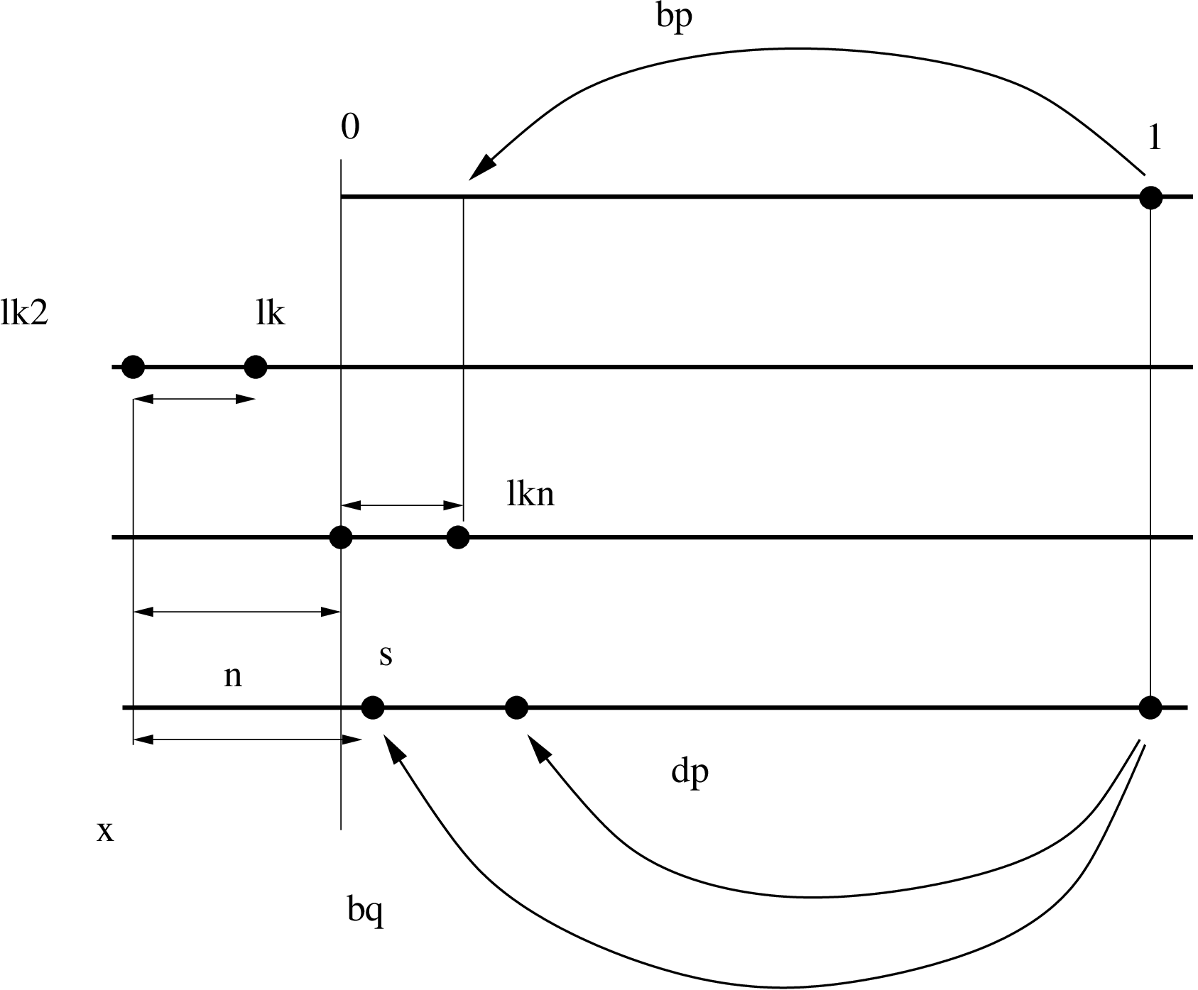
To complete the proof we just need to choose arbitrarily small $\xi$ and a new $\bar{\beta}$ (close to $\hat{\beta}$ ) such that

\bar{\beta}^{-q}=\xi\quad\mbox{and}\quad\bar{\beta}^{p}\,(-|\lambda^{k}|+|\lambda|^{k-2}+\xi)=1.

Then for $\nu=\hat{\nu}+\xi$ the following equations hold simultaneously (see Figure 3):

\bar{\beta}^{-q}=\xi\quad\Rightarrow\quad f_{\bar{\beta}}^{q}\circ T^{\operatorname{c}}_{(a,b),\hat{\nu}+\xi}\circ f_{\lambda}^{k-2}\circ T^{\operatorname{c}}_{(b,a)}(1)=1

for some $q=q(\xi)$ , $q(\xi)\to\infty$ as $\xi\to 0$ , and

\bar{\beta}^{p}\,(-|\lambda^{k}|+|\lambda|^{k-2}+\xi)=1\quad\Rightarrow\quad f_{\bar{\beta}}^{p}\circ T^{\operatorname{c}}_{(a,b),\hat{\nu}+\xi}\circ f_{\lambda}^{k}\circ T^{\operatorname{c}}_{(b,a)}(1)=1.

This completes the proof of the lemma. ∎

Notice that, using the notation above, there are two periodic points for $f_{\nu}$ , $R_{k,p}$ and $R_{k-2,q}$ .

We now explain our choice of the periodic point $R_{\ell,m}$ . This choice depends on whether or not the map $T^{\operatorname{c}}_{(a,b)}$ preserves the orientation, and is done bearing in mind that we want to get periodic points $R_{\ell,m}$ with uniformly bounded (with respect to $\ell$ and $m$ chosen in a specified way) central multipliers.

First, if $T^{{\operatorname{c}}}_{(a,b)}$ is orientation preserving then we let $\ell=k$ and $m=p$ . To calculate the central multiplier of $R_{\ell,m}$ note that $\lambda^{\ell}=|\lambda^{\ell}|$ ( $\ell=k$ is even) and that, in this case, $f_{\bar{\beta}}^{m}\circ T^{\operatorname{c}}_{(a,b),\nu}\circ f_{\lambda}^{\ell}\circ T^{\operatorname{c}}_{(b,a)}(1)=1$ for $\nu=|\lambda^{\ell-2}|+\xi$ means

\bar{\beta}^{m}\,(-|\lambda^{\ell}|+|\lambda|^{\ell-2}+\xi)=1\quad\Rightarrow\quad|\bar{\beta}^{m}\,\lambda^{\ell}|=\frac{(1-\bar{\beta}^{m}\,\xi)\,\lambda^{2}}{1-\lambda^{2}}.

(8)

In the reversing orientation case, we let $\ell=k-2$ and $m=q$ . In this case, $f_{\bar{\beta}}^{m}\circ T^{\operatorname{c}}_{(a,b),\nu}\circ f_{\lambda}^{\ell}\circ T^{\operatorname{c}}_{(b,a)}(1)=1$ for $\nu=-|\lambda^{\ell+2}|+\xi$ implies that

\bar{\beta}^{m}\,(|\lambda^{\ell}|-|\lambda|^{\ell+2}+\xi)=1\quad\Rightarrow\quad|\bar{\beta}^{m}\,\lambda^{\ell}|=\frac{(1-\bar{\beta}^{m}\,\xi)}{1-\lambda^{2}}.

(9)

Notice that here we used essentially the specific choice of $\ell$ and $m$ above. Notice also that in both cases the choice of $\ell$ and $m$ can be done before the choice of $\xi$ . Thus, for chosen $m$ and $\ell$ , taking small $\xi$ implies that the absolute value of the central multiplier of $R_{\ell,m}$ (which is $|\bar{\beta}^{m}\,\lambda^{\ell}|$ ) is uniformly bounded (independently of chosen $\ell$ and $m$ ). Finally, we get the following statement.

Lemma 4.16.

There is $\Theta>0$ such that the absolute value of the central multiplier of the point $R_{\ell,m}$ satisfies ${\Theta}^{-1}<|\lambda^{\operatorname{c}}(R_{\ell,m})|<\Theta$ , for all large $\ell$ and $m$ chosen as above. Therefore, the saddle $R_{\ell,m}$ satisfies item 2) in Proposition 4.5.

4.5 Proofs of Propositions 4.5 and 4.3

4.5.1 Proof of Proposition 4.5

Consider the partially hyperbolic neighborhood $V$ in (4) in Lemma 4.12 and the sequence of parameters $\nu_{k}$ in Lemma 4.15. Let $R_{k}$ be the periodic point of $f_{\nu_{k}}$ given by Lemma 4.13 (with the notation of this lemma, $R_{k}=R_{\ell_{k},m_{k}}$ ). We claim that these saddles satisfy the conclusions in Proposition 4.5. The period of $R_{k}$ is given by Lemma 4.8 and the estimate on the central multiplier and the itinerary of this saddle are provided by Lemma 4.16. Finally, since the splitting of $\Lambda_{f_{k}}(V)$ consists of one-dimensional directions (Lemma 4.12) this saddle has real multipliers.

Taking small $\xi>0$ in equations (8) and (9) and noting that $m$ remains fixed and $\lambda=\lambda^{\operatorname{c}}(A_{f})$ is close to one, one gets that $R_{k}$ and $B_{f}$ have the same index.

The intersection properties in items 3)–5) follow from Lemmas 4.11 and 4.13, as stated in Remark 4.14. This concludes the proof of Proposition 4.5. $\Box$

4.5.2 Proof of Proposition 4.3

The proof of Proposition 4.3 follows from the previous constructions and the ones in [BD4], where it is proved that every co-index one cycle generates robust cycles ¹⁰¹⁰ 10 Consider $f$ with a co-index one cycle, then there is a $C^{1}$ -open set ${\cal U}$ whose closure contains $f$ such that very $g\in{\cal U}$ has transitive hyperbolic sets $\Lambda_{g}$ and $\Sigma_{g}$ of different indices such that $W^{u}(\Sigma_{g})\cap W^{s}(\Lambda_{g})\neq\emptyset$ and $W^{s}(\Sigma_{g})\cap W^{u}(\Lambda_{g})\neq\emptyset$ . Necessarily, at least one of these sets is non-trivial.. The key step of the construction in [BD4] is to obtain a partially hyperbolic saddle $S$ with a real multiplier close to one having a strong stable/unstable connexion $W^{\operatorname{ss}}(S)\cap W^{\operatorname{uu}}(S)\neq\emptyset$ , exactly as the points $R_{k}$ in Proposition 4.5 (note that, a priori, the central multiplier of $R_{k}$ is not close to one). Such a dynamical configuration generates cycles via a blender-like construction that we will explain below. As the existence of a blender structure is open (see [BD1, Lemma 1.11]), we can explain the proof for a special linear perturbation. We will follow the model in [BDV1]. For a discussion of the notion of blender see [BDV2, Chapter 6.2]. We now go to the details of this construction.

Applying Proposition 4.5 to the partially hyperbolic neighborhood $V$ , we get a sequence of diffeomorphisms $f_{k}$ converging to $f$ such that every $f_{k}$ has a saddle $R_{k}$ satisfying the conclusions of Proposition 4.5. To get these saddles having central multipliers with modulus close to one we use the following lemma:

Lemma 4.17 (Franks’ Lemma, [F]).

Consider a diffeomorphism $f$ and an $\varepsilon$ -perturbation $A$ of the derivative $Df$ of $f$ along an $f$ -invariant finite set $\Sigma$ . Then, for every neighborhood $U$ of $\,\Sigma$ , there is a diffeomorphism $g$ $C^{1}$ - $\varepsilon$ -close to $f$ such that $g(x)=f(x)$ , if $x\in\Sigma$ or if $x\not\in U$ , and $Dg(x)=A(x)$ , for all $x\in\Sigma$ .

Recall that the periods $\pi(R_{k})$ go to infinity as $k\to\infty$ and that the central multipliers $|\lambda^{\operatorname{c}}(R_{k})|$ are uniformly bounded. To get a saddle $R_{k}$ (satisfying Proposition 4.5) whose central multiplier has modulus close to $1$ it is enough to consider a multiplication in the central direction along the orbit of $R_{k}$ by a factor $(1+\varepsilon)\,|\lambda^{\operatorname{c}}(R_{k})|^{-1/\pi(R_{k})}$ (which is close to $(1+\varepsilon)$ for large $k$ ) preserving the partially hyperbolic splitting and apply Lemma 4.17.

We now proceed to explain the blender-like construction when the multiplier of $R_{k}$ is positive (see [BD4] for the negative case)¹¹¹¹ 11 In fact, our construction can be modified to get the saddles $R_{k}$ in Proposition 4.5 having positive central multipliers, but this construction is much more involved.. Assume that, in our local coordinates, the point $R=R_{k}=(0^{s},0,0^{u})$ and that the local dynamics at $R$ is linear, $f(x^{s},x,x^{u})=(A^{\operatorname{s}}(x^{s}),\sigma\,x,A^{\operatorname{u}}(x^{u}))$ , where $A^{\operatorname{s}}$ is a contracting matrix, $A^{\operatorname{u}}$ is expanding, and $\lambda^{\operatorname{c}}(R)=\sigma\in(1,2)$ . By 4) in Proposition 4.5, there is a strong stable/unstable intersection associated to $R$ : there are a small disk $D^{\operatorname{u}}\subset\{(0^{s},0)\}\times[-1,1]^{u}\subset W^{\operatorname{u}}(R)$ and $k_{0}$ such that $f^{k_{0}}(D^{\operatorname{u}})=\{(\kappa^{s}_{0},0)\}\times[-1,1]^{u}$ (the first $k_{0}$ iterates of $D^{\operatorname{u}}$ are contained in ${V_{0}}$ ). We consider a one parameter family of diffeomorphisms (perturbations of $f$ in a neighborhood of $D^{\operatorname{u}}$ ) such that if $(x^{s},x,x^{u})$ is in a neighborhood of $D^{\operatorname{u}}$ then

f_{t}^{k_{0}}(x^{s},x,x^{u})=f(x^{s},x,x^{u})+(0^{s},t,0^{u}).

Consider $t<0$ and the cube

C=[-1,1]^{s}\times[0,|t|/(\sigma-1)]\times[-1,1]^{u}\subset V

Now [BDV1, lemma in page 717] implies the following intersection property:

Intersection property: Consider the disk $\Delta^{\operatorname{u}}_{[\rho_{1},\rho_{2}]}=\{d_{0}^{s}\}\times[\rho_{1},\rho_{2}]\times[-1,1]^{u}\subset C$ , $\rho_{1}<\rho_{2}$ . Then there is a point $X$ of transverse intersection between $W^{{\operatorname{s}}}(R)$ and $\Delta^{\operatorname{u}}_{[\rho_{1},\rho_{2}]}$ whose forward orbit is contained in $V$ , see Figure 4.

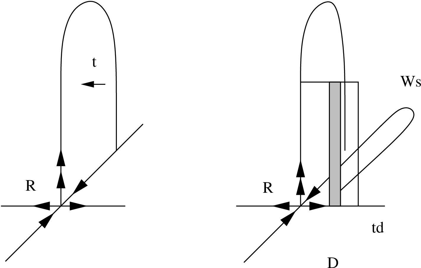
Since we have $B\,\cap_{{\operatorname{s}},\operatorname{uu},V}\,R$ and $A\,\cap_{{\operatorname{u}},{\operatorname{s}},V}\,R$ (recall items 4) and 5) of Proposition 4.5), there are compact disks $K^{\operatorname{s}}(B)\subset W^{\operatorname{s}}(B)$ and $K^{\operatorname{u}}(A)\subset W^{\operatorname{u}}(A)$ (contained in $V$ ) close to $W^{{\operatorname{s}}}_{{\operatorname{loc}}}(R)$ and $W^{\operatorname{uu}}_{{\operatorname{loc}}}(R)$ , respectively. We can now consider a local perturbation $g$ of $f_{t}$ (in a domain different of the family of perturbations $f_{t}$ ) such that in the local coordinates at $R$ one has (see Figure 5)

\begin{array}[]{ll}K^{\operatorname{u}}(A)&=\{(a_{0}^{s},a_{0})\}\times[-1,1]^{u},\quad a_{0}\in(0,|t|/(\sigma-1));\\ K^{\operatorname{s}}(B)&=[-1,1]^{s}\times\{(b_{0},b^{u}_{0})\},\quad b_{0}<0.\end{array}

Finally, the disk $K^{\operatorname{u}}(A)$ intersects the cube $C$ from the bottom to the top. And this holds for the continuation of $K^{\operatorname{u}}(A_{h})$ for every $h$ close to $g$ . This implies that there is a $C^{1}$ -neighborhood ${\cal E}$ of $g$ such that (by the intersection property) $K^{\operatorname{u}}(A_{h})$ is $V$ -accumulated by the stable manifold of $R_{h}$ . Therefore densely in ${\cal E}$ one can obtain $V$ -related cycles associated to $R_{h}$ and $A_{h}$ . Since $B_{h}$ is $V$ -homoclinically related to $R_{h}$ , one also has $V$ -related cycles associated to $B_{h}$ and $A_{h}$ . This completes the proof of Proposition 4.3. $\Box$

5 Final construction

In this section we use the results of previous sections to complete the proof of Theorem 1.

Let $\mathcal{G}$ be the residual set of $\text{\rm Diff}^{\,1}(M)$ described in Section 3.1. The statement below is a local version of Theorem 1.

Theorem 2.

Let $f\in\mathcal{G}$ have two hyperbolic saddles $P_{f}$ and $Q_{f}$ of different indices in the same homoclinic class. Arbitrarily $C^{1}$ -close to $f$ there exists a $C^{1}$ -open set $\mathcal{Z}\subset\text{\rm Diff}^{\,1}(M)$ and a residual subset $\mathcal{R}\subset\mathcal{Z}$ such that every $g\in\mathcal{R}$ has a non-hyperbolic ergodic invariant measure with uncountable support inside of the homoclinic class of $P_{g}$ and $Q_{g}$ .

Remark 5.1.

The genericity hypothesis imply that $H(P_{g},g)=H(Q_{g},g)$ .

Due to standard genericity arguments Theorem 2 implies Theorem 1, for details see [ABCDW].

The genericity hypothesis imply that the map $f$ has two saddles with real multipliers of consecutive indices, say $A_{f}$ and $B_{f}$ , $\text{\rm index}(A_{f})+1=\text{\rm index}(B_{f})$ , such that the saddle $A_{f}$ is homoclinically related to $P_{f}$ and the saddle $B_{f}$ is homoclinically related to $Q_{f}$ . Moreover, we can assume that the saddle $A_{f}$ is ${\operatorname{s}}$ -biaccumulated, the saddle $B_{f}$ is ${\operatorname{u}}$ -biaccumulated, and that the central multiplier of $A_{f}$ is close to one (it is enough to have $|\lambda^{{\operatorname{c}}}(A_{f})|\in(0.9,1)$ ), see generic conditions R3)–R4).

We proceed as follows:

•

Proposition 3.5 implies that by a $C^{1}$ -perturbation we can create a cycle corresponding to the continuations of the saddles $A_{f}$ and $B_{f}$ .
•

Apply Lemma 4.2 to this cycle. This gives a map $g$ which is $C^{1}$ -close to $f$ , and an open set $V\subseteq M$ such that $\Lambda_{g}(V)$ is strongly partially hyperbolic (one dimensional central manifold), $A_{g}$ is ${V}$ - ${\operatorname{s}}$ -biaccumulated and $B_{g}$ is ${V}$ - ${\operatorname{u}}$ -biaccumulated, and $g$ has a $V$ -related cycle associated to $A_{g}$ and $B_{g}$ .
•

By Proposition 4.3, $C^{1}$ -near there is an open set $\mathcal{Z}$ and a dense in $\mathcal{Z}$ countable subset $\mathcal{D}\subset\mathcal{Z}$ such that every $g\in\mathcal{D}$ has a $V$ -related cycle associated with the saddles $A_{g}$ and $B_{g}$ .

From now on we fix the open set $\mathcal{Z}\subset\text{\rm Diff}^{\,1}(M)$ , the countable dense subset $\mathcal{D}$ of $\mathcal{Z}$ , the saddles $A_{g}$ and $B_{g}$ , and the neighborhood $V\subset M$ .

Proposition 5.2.

Generic diffeomorphisms from $\mathcal{Z}$ have a sequence of periodic saddles in $V$ which satisfies the assumptions of Proposition 2.5 and belongs to the continuation of the homoclinic class above.

Note that Propositions 5.2 and 2.5 imply the existence of non-hyperbolic ergodic measures for generic diffeomorphisms from $\mathcal{Z}$ , and, thus, Theorem 2.

For any $g\in\mathcal{Z}$ the maximal invariant set $\Lambda_{g}=\cap_{k\in\mathbb{Z}}g^{k}(V)$ is a (not necessarily closed) partially hyperbolic invariant set (with a splitting $E^{\operatorname{ss}}\oplus E^{\operatorname{c}}\oplus E^{\operatorname{uu}}$ , $E^{\operatorname{c}}$ is one-dimensional). For $g\in\mathcal{Z}$ denote by $\chi^{{\operatorname{c}}}(A_{g})<0$ and $\chi^{{\operatorname{c}}}(B_{g})>0$ the central Lyapunov exponents of saddles $A_{g}$ and $B_{g}$ (corresponding to the central direction $E^{{\operatorname{c}}}$ ). Fix a constant $C$ such that

C>\sup_{g\in\mathcal{Z}}\displaystyle{\frac{16}{|\chi^{{\operatorname{c}}}(A_{g})|}}.

(10)

Proposition 5.3.

For each $N\in\mathbb{N}$ there is a family of open sets $\mathcal{Z}_{n_{1},\ldots,n_{N}}\subseteq\mathcal{Z}$ indexed by $N$ -tuples $(n_{1},\ldots,n_{N}),\ n_{i}\in\mathbb{N},$ satisfying the following properties:

Z1) For any tuples $(n_{1},\ldots,n_{N})\neq(m_{1},\ldots,m_{N})$ the sets $\mathcal{Z}_{n_{1},\ldots,n_{N}}$ and $\mathcal{Z}_{m_{1},\ldots,m_{N}}$ are disjoint.

Z2) For any tuple $(n_{1},\ldots,n_{N},n_{N+1})$ we have $\mathcal{Z}_{n_{1},\ldots,n_{N},n_{N+1}}\subseteq\mathcal{Z}_{n_{1},\ldots,n_{N}}.$ In particular, $\mathcal{Z}_{n_{1}}\subseteq\mathcal{Z}$ for every $n_{1}\in\mathbb{N}$ .

Z3) The union $\cup_{n_{1}\in{\mathbb{N}}}\mathcal{Z}_{n_{1}}$ is dense in $\mathcal{Z}$ , and for each $N$ the union $\cup_{j\in\mathbb{N}}\mathcal{Z}_{n_{1},\ldots n_{N},j}$ is dense in $\mathcal{Z}_{n_{1},\ldots,n_{N}}$ .

Z4) Every diffeomorphism $g\in\mathcal{Z}_{n_{1},\ldots,n_{N}}$ has a finite sequence of periodic saddles homoclinically related to $B_{g}$ (thus of the same index as $B_{g}$ )

\{P_{n_{1}},P_{n_{1},n_{2}},\ldots,P_{n_{1},n_{2},\ldots,n_{N}}\}\subset\Lambda_{g}\cap H(B_{g},g)

having real multipliers, satisfying the $V$ - ${\operatorname{u}}$ -biaccumulation property, and of growing periods, $\pi(B_{g})<\pi(P_{n_{1}})<\ldots<\pi(P_{n_{1},n_{2},\dots,n_{N}})$ . Moreover, saddles $\{P_{n_{1}},P_{n_{1},n_{2}},\ldots,P_{n_{1},n_{2},\ldots,n_{N}}\}$ depend continuously on $g$ when $g$ varies over $\mathcal{Z}_{n_{1},\ldots,n_{N}}$ .

Z5) For any tuple $(n_{1},\ldots,n_{N})$ there exists a countable dense subset $\mathcal{D}_{n_{1},\ldots,n_{N}}\subset\mathcal{Z}_{n_{1},\ldots,n_{N}}$ such that every $g\in\mathcal{D}_{n_{1},\ldots,n_{N}}$ has a $V$ -related heterodimensional cycle associated to the saddles $A_{g}$ and $P_{n_{1},\ldots,n_{N}}$ .

Z6) There are numbers $\{\gamma_{n_{1},\ldots,n_{N}}\}_{(n_{1},\ldots,n_{N})\in\mathbb{N}^{N}}$ such that for any $N\in\mathbb{N}$ , any tuple $(n_{1},\ldots,n_{N},n_{N+1})$ , and any $g\in\mathcal{Z}_{n_{1},\ldots,n_{N},n_{N+1}}$ the orbit of $P_{n_{1},\ldots,n_{N},n_{N+1}}$ is a $(\gamma_{n_{1},\ldots,n_{N}},1-C\,|\chi^{c}(P_{n_{1},\ldots,n_{N}})|)$ -good approximation of the orbit of $P_{n_{1},\ldots,n_{N}}$ (recall Definition 2.4), where $C$ is the constant in (10).

Z7) Take any $g\in\mathcal{Z}_{n_{1},\ldots,n_{N}}$ . Let $d_{k},1\leq k\leq N$ , be the minimal distance between the points of the $g$ -orbit of $P_{n_{1},\ldots,n_{k}}$ . Then

\gamma_{n_{1},\ldots,n_{N}}<\frac{\min_{1\leq k\leq N}d_{k}}{3\cdot 2^{N}}.

Z8) For any $N\in\mathbb{N}$ , any tuple $(n_{1},\ldots,n_{N},n_{N+1})$ , and any $g\in\mathcal{Z}_{n_{1},\ldots,n_{N},n_{N+1}}$

|\chi^{c}(P_{n_{1},\ldots,n_{N},n_{N+1}})|<\frac{1}{2}\,|\chi^{c}(P_{n_{1},\ldots,n_{N}})|.

Before proving Proposition 5.3 let us complete the proof of Proposition 5.2 (and, therefore, of the main result).

Due to Property Z3), for any $N\in\mathbb{N}$ the set $\widetilde{\mathcal{Z}}_{N}=\cup_{(n_{1},\ldots,n_{N})\in\mathbb{N}^{N}}\mathcal{Z}_{n_{1},\ldots,n_{N}}$ is an open and dense subset of $\mathcal{Z}$ . Consider the intersection $\mathcal{R}=\cap_{N\in\mathbb{N}}\widetilde{\mathcal{Z}}_{N}$ . The set $\mathcal{R}$ is a residual subset of $\mathcal{Z}$ . Take any $g\in\mathcal{R}$ . Property Z1) implies that for each $N\in{\mathbb{N}}$ the map $g$ belongs to one and only one set from the collection $\{\mathcal{Z}_{n_{1},\ldots,n_{N}}\}_{(n_{1},\ldots,n_{N})\in{\mathbb{N}}^{N}}$ . Therefore, due to Z2) and Z4), for the diffeomorphism $g\in\mathcal{R}$ a sequence of periodic points $\{B_{g},P_{n_{1}},P_{n_{1},n_{2}}\ldots,P_{n_{1},n_{2},\ldots,n_{N}},\ldots\}\subset\Lambda_{g}\cap H(B_{g},g)$ is well defined. We claim that this sequence satisfies the assumptions of Proposition 2.5.

Indeed, assumptions 1) and 2) follows from the choice of the set $V\subset M$ and Property Z4). Assumptions 3), 4), and 5) follow from Z6), Z7), and Z8), respectively. This proves Proposition 5.2, and an application of Proposition 2.5 now implies Theorem 2 (and, hence, Theorem 1).

Proof of Proposition 5.3.

Let us first construct sets $\mathcal{Z}_{n_{1}}\subset\mathcal{Z},n_{1}\in\mathbb{N}$ . The subset $\mathcal{D}\subset\mathcal{Z}$ (consisting of diffeomorphisms with cycles) is countable. Let us enumerate diffeomorphisms from $\mathcal{D}=\{g_{i}\}_{i\in\mathbb{N}}$ . Take one of these diffeomorphisms, say, $g_{i}\in\mathcal{D}$ .

Denote by ${\cal O}(P)$ the orbit of a point $P$ . Choose a constant $\gamma>0$ such that

\gamma<\inf_{g\in\mathcal{Z}}\ \ \min_{X,Y\in\mathcal{O}(B_{g}),\ X\neq Y}\frac{1}{3}\,\text{\rm dist}(X,Y).

(11)

Denote by $\lambda<1$ the central multiplier of the saddle $A_{g_{i}}$ , and by $\beta>1$ the central multiplier of the saddle $B_{g_{i}}$ . Choose a neighborhood $\mathcal{U}(g_{i})\subset\text{\rm Diff}^{\,1}(M)$ and small (in particular, each component is of radius smaller than $\gamma$ ) neighborhoods $U_{A_{g_{i}}}$ , and $U_{B_{g_{i}}}\subset M$ of the orbits of $A_{g_{i}}$ and $B_{g_{i}}$ such that

\forall g\in\mathcal{U}(g_{i})\ \forall x\in U_{A_{g_{i}}}\colon\quad\lambda^{2}\leq\|Df^{\pi(A_{g_{i}})}|_{E^{c}}(x)\|\leq\lambda^{\frac{1}{2}}

(12)

and

\forall g\in\mathcal{U}(g_{i})\ \forall x\in U_{B_{g_{i}}}\colon\quad\beta^{\frac{1}{2}}\leq\|Df^{\pi(B_{g_{i}})}|_{E^{c}}(x)\|\leq\beta^{2}.

(13)

Proposition 4.5 allows to obtain a sequence of diffeomorphisms $g_{ik}$ , $g_{ik}\to g_{i}$ as $k\to\infty$ , such that each diffeomorphism $g_{ik}$ has a periodic saddle $S_{ik}$ with real multipliers (denoted by $R_{k}$ in Proposition 4.5), having the following properties:

S1) the saddle $S_{ik}$ is $V$ -homoclinically related to $B_{g_{ik}}$ , thus has the same index as $B_{g_{i}}$ ;

S2) for some constant $\Theta$ that does not depend on $k$ and for each $k\in\mathbb{N}$ we have $1<|\lambda^{c}(S_{ik})|<\Theta$ ;

S3) the map $g_{ik}$ has a $V$ -related cycle associated to $S_{ik}$ and $A_{g_{ik}}$ ;

S4) there are sequences of natural numbers $\ell_{k},m_{k}$ that tend to infinity as $k\to\infty$ , such that under the iterates of $g_{ik}$ the saddle $S_{ik}$ needs a fixed number of iterates (independent of $k$ ) to go from a neighborhood $U_{B_{g_{i}}}$ to a neighborhood $U_{A_{g_{i}}}$ , then it remains $\ell_{k}\,\pi(A_{g_{i}})$ iterates in $U_{A_{g_{i}}}$ , then it needs a fixed number of iterates to go from $U_{A_{g_{i}}}$ to $U_{B_{g_{i}}}$ , and finally it remains $m_{k}\,\pi(B_{g_{i}})$ iterates in $U_{B_{g_{i}}}$ . In particular, there is a constant $t\in{\mathbb{N}}$ independent of $k$ such that

\pi(S_{ik})=m_{k}\,\pi(B_{g_{i}})+\ell_{k}\,\pi(A_{g_{i}})+t.

Moreover, properties (3) and (4) from Proposition 4.5 guarantee that making an arbitrary small perturbation of $g_{ik}$ (preserving properties S1) - S4)) we can obtain an additional property:

: S5) the saddle $S_{ik}$ has the $V$ - ${\operatorname{u}}$ -biaccumulation property.

Lemma 5.4.

For every large $k\in\mathbb{N}$ the saddles $S_{ik}$ also have the following properties:

0<\chi^{c}(S_{ik})<\frac{1}{2}\chi^{c}(B_{g_{ik}}),

(14)

\frac{m_{k}\pi(B_{g_{i}})}{m_{k}\pi(B_{g_{i}})+\ell_{k}\pi(A_{g_{i}})+t}>1-C\chi^{c}(B_{g_{ik}}).

(15)

Proof.

If $k$ is large enough then $g_{ik}\in\mathcal{U}(g_{i}).$ Let us show that for large $k$ the inequality (14) holds. On the one hand, from S2) and S4) we have

0<\chi^{c}(S_{ik})\leq\frac{\log\Theta}{\pi(S_{ik})}=\frac{\log\Theta}{m_{k}\,\pi(B_{g_{i}})+\ell_{k}\,\pi(A_{g_{i}})+t}\to 0\ \ \ \text{\rm as}\ \ \ \ k\to\infty.

On the other hand, due to (13), $0<\dfrac{\log\beta^{\frac{1}{2}}}{\pi(B_{g_{i}})}\leq\chi^{c}(B_{g_{ik}}).$ This implies that (14) holds for large $k$ .

Now let us prove that (15) also holds for large enough $k\in{\mathbb{N}}$ . Due to (12) and (13), using S4), the central multiplier of $S_{ik}$ can be estimated from above,

1<|\lambda^{c}(S_{ik})|\leq|(\beta^{2})^{m_{k}}(\lambda^{\frac{1}{2}})^{\ell_{k}}T|,

where $T$ is a constant (that does not depend on $k$ ) which is responsible for the part of the orbit of $S_{ik}$ outside of neighborhoods $U_{A_{g_{i}}}$ and $U_{B_{g_{i}}}$ which does not depend on $k$ . This implies that

\ell_{k}<-\frac{\log T}{\log\lambda^{\frac{1}{2}}}-\frac{m_{k}\log\beta^{2}}{\log\lambda^{\frac{1}{2}}}.

From this estimate for every large $k$ we have

\begin{array}[]{ll}&1-\dfrac{m_{k}\pi(B_{g_{i}})}{m_{k}\pi(B_{g_{i}})+\ell_{k}\pi(A_{g_{i}})+t}=\dfrac{\ell_{k}\pi(A_{g_{i}})+t}{m_{k}\pi(B_{g_{i}})+\ell_{k}\pi(A_{g_{i}})+t}\leq\dfrac{\ell_{k}\pi(A_{g_{i}})+t}{m_{k}\pi(B_{g_{i}})}\leq\\ &\qquad\qquad\leq\dfrac{1}{m_{k}}\left(\dfrac{t}{\pi(B_{g_{i}})}-\dfrac{\log T}{\log\lambda^{\frac{1}{2}}}\cdot\dfrac{\pi(A_{g_{i}})}{\pi(B_{g_{i}})}\right)-4\,\dfrac{\log\beta}{\log\lambda}\cdot\dfrac{\pi(A_{g_{i}})}{\pi(B_{g_{i}})}=\\ &\qquad\qquad=\dfrac{1}{m_{k}}\left(\dfrac{t}{\pi(B_{g_{i}})}-\dfrac{\log T}{\log\lambda^{\frac{1}{2}}}\cdot\dfrac{\pi(A_{g_{i}})}{\pi(B_{g_{i}})}\right)-4\,\dfrac{\chi^{c}(B_{g_{i}})}{\chi^{c}(A_{g_{i}})}<8\,\dfrac{\chi^{c}(B_{g_{i}})}{|\chi^{c}(A_{g_{i}})|}.\end{array}

Finally, due to the choice of the constant $C$ defined by (10),

1-\dfrac{m_{k}\pi(B_{g_{i}})}{m_{k}\pi(B_{g_{i}})+\ell_{k}\pi(A_{g_{i}})+t}<\frac{1}{2}\,C\chi^{c}(B_{g_{i}})<C\,\chi^{c}(B_{g_{ik}}).

This completes the proof of the lemma. ∎

Consider now the set

\mathcal{D^{\prime}}=\left\{g_{ik}\ |\ S_{ik}\text{\rm\ \ satisfies conditions (\ref{e.1}), (\ref{e.2})}\right\}\subset\mathcal{Z}.

By construction, the set $\mathcal{D^{\prime}}$ is a countable dense subset of $\mathcal{Z}$ . Let us enumerate the elements of $\mathcal{D^{\prime}}=\{h_{n_{1}}\}_{n_{1}\in{\mathbb{N}}}$ . Let us also redenote by $P_{n_{1}}$ the periodic saddle $S_{ik}$ of the map $h_{n_{1}}\equiv g_{ik}$ . For each $h_{n_{1}}$ we can apply Proposition 4.3 to the heteroclinic $V$ -related cycle associated to saddles $P_{n_{1}}$ and $A_{h_{n_{1}}}$ . This gives for each $n_{1}\in{\mathbb{N}}$ an open set $\mathcal{U}_{n_{1}}\subseteq\mathcal{Z}$ and a dense countable subset $\widetilde{\mathcal{D}}_{n_{1}}\subset\mathcal{U}_{n_{1}}$ such that $h_{n_{1}}\in\overline{\mathcal{U}}_{n_{1}}$ and every $g\in\widetilde{\mathcal{D}}_{n_{1}}$ has a $V$ -related cycle associated with $A_{g}$ and a continuation of $P_{n_{1}}$ . In order to simplify the notation, we will omit the dependence of the continuation of $P_{n_{1}}$ on $g$ and will write just $P_{n_{1}}$ instead of “continuation of $P_{n_{1}}$ ”. We can take $\mathcal{U}_{n_{1}}$ small enough to guarantee that for every $g\in\mathcal{U}_{n_{1}}$ one has $0<\chi^{c}(P_{n_{1}})<\frac{1}{2}\chi^{c}(B_{g})$ . Indeed, due to (14) this inequality holds for $h_{n_{1}}$ . Since Lyapunov exponents of a hyperbolic saddle depend continuously on a diffeomorphism, the inequality holds also for all $g$ sufficiently $C^{1}$ -close to $h_{n_{1}}$ .

Let us now take inductively

\mathcal{Z}_{1}=\mathcal{U}_{1},\ \mathcal{Z}_{2}=\mathcal{U}_{2}\backslash\overline{\mathcal{Z}}_{1},\ldots,\mathcal{Z}_{n_{1}}=\mathcal{U}_{n_{1}}\backslash\overline{\mathcal{Z}}_{n_{1}-1},\ldots

and

\mathcal{D}_{n_{1}}=\widetilde{\mathcal{D}}_{n_{1}}\cap\mathcal{Z}_{n_{1}},n_{1}\in{\mathbb{N}}.

We claim that the collection of sets $\{\mathcal{Z}_{n_{1}}\}_{n_{1}\in{\mathbb{N}}}$ satisfies the required properties Z1) - Z8).

•

Properties Z1) and Z2) directly follow from the construction of $\{\mathcal{Z}_{n_{1}}\}_{n_{1}\in{\mathbb{N}}}$ .
•

Since the set $\{h_{n_{1}}\}_{n_{1}\in{\mathbb{N}}}$ is dense in $\mathcal{Z}$ , the union $\cup_{n_{1}\in{\mathbb{N}}}\mathcal{U}_{n_{1}}$ is dense in $\mathcal{Z}$ , and hence $\cup_{n_{1}\in{\mathbb{N}}}\mathcal{Z}_{n_{1}}$ is also dense in $\mathcal{Z}$ , so Z3) holds.
•

For each $g\in\mathcal{Z}_{n_{1}}$ saddle $\{P_{n_{1}}\}_{n_{1}\in{\mathbb{N}}}$ is $V$ -homoclinically related to $B_{g}$ , has real multipliers, $V$ - ${\operatorname{u}}$ -biaccumulation property, and $\pi(B_{g})<\pi(P_{n_{1}})$ , so Z4) holds.
•

The sets $\mathcal{D}_{n_{1}}\subset\mathcal{Z}_{n_{1}}$ were constructed to satisfy Z5).
•

Take $g\in\mathcal{Z}_{n_{1}}$ , and denote by $\Gamma$ the part of the orbit of $P_{n_{1}}$ that belongs to the neighborhood $U_{B_{g}}$ . Define the projection

$\rho:\Gamma\to\mathcal{O}(B_{g}),\quad\rho(x)=\{\text{\rm the point of $\mathcal{O}(B_{g})$ nearest to $x$}\}.$

By construction,

$\#\Gamma=m_{k}\pi(B_{g})\quad\mbox{and}\quad\#(\mathcal{O}(P_{n_{1}}))=m_{k}\pi(B_{g})+\ell_{k}\pi(A_{g})+t.$

Recall that here $k$ and $n_{1}$ are related due to the enumeration $h_{n_{1}}=g_{ik}$ ; notice that in fact integers $m_{k}$ , $\ell_{k}$ , and $t$ depend also on the index $i$ , but our notations do not reflect this dependence. Now Z6) follows from the inequality (15) and the choice of $\gamma$ in (11).
•

The value of $\gamma$ could be taken arbitrary small; in particular Z7) can be satisfied by the choice of sufficiently small $\gamma$ (that choice was explicitly specified in (11)).
•

The last property Z8) follows directly from the inequality (14).

Finally, assume that the sets $\{\mathcal{Z}_{n_{1},\ldots,n_{N}},n_{i}\in\mathbb{N}\}$ were constructed. Take one of these sets, say, $\mathcal{Z}_{n_{1},\ldots,n_{N}}$ . Exactly the same arguments that we used to construct the sets $\mathcal{Z}_{n_{1}}\subset\mathcal{Z},n_{1}\in\mathbb{N}$ , can be now used to construct the sets $\mathcal{Z}_{n_{1},\ldots,n_{N},n_{N+1}}\subseteq\mathcal{Z}_{n_{1},\ldots,n_{N}},n_{N+1}\in\mathbb{N}$ . By induction, Proposition 5.3 follows. ∎

References

[ABC] F. Abdenur, Ch. Bonatti, S. Crovisier, Nonuniform hyperbolicity for $C^{1}$ -generic diffeomorphisms, in preparation.
[ABCD] F. Abdenur, Ch. Bonatti, S. Crovisier, L. J. Díaz, Generic diffeomorphisms on compact surfaces, Fundamenta Math., 187 (2005), pp. 127–159.
[ABCDW] F. Abdenur, Ch. Bonatti, S. Crovisier, L. J. Díaz, L. Wen, Periodic points and homoclinic classes, Ergodic Th. and Dynam. Syst., 26 (2006), pp. 1–22,
[AD] F. Abdenur, L. J. Díaz, Pseudo-orbit shadowing in the $C^{1}$ -topology, Discrete Contin. Dyn. Syst., 17 (2007), pp. 223–245.
[AS] R. Abraham, S. Smale, Nongenericity of $\Omega$ -stability. In: Global Analysis (Proc. Sympos. Pure Math., Vol. XIV, Berkeley, Calif., 1968), Amer. Math. Soc., Providence, R.I., 1970, pp. 5–8.
[AAS] J. Alves, V. Araújo, B. Saussol, On the uniform hyperbolicity of some nonuniformly hyperbolic systems. Proc. Amer. Math. Soc., 131 (2003), pp. 1303–1309.
[A] N. Aoki, The set of axiom A diffeomorphisms with no cycles, Bol. Soc. Bras. Mat. (N.S.), 23 (1992), pp. 21–65.
[BB] A. Baraviera, Ch. Bonatti, Removing zero Lyapunov exponents, Ergodic Th. and Dynam. Systems, 23 (2003), pp. 1655–1670.
[B] J. Bochi, Genericity of zero Lyapunov exponents, Ergodic Th. and Dynam. Systems, 22 (2002), pp. 1667–1696.
[BcV] J. Bochi, M. Viana, Uniform (projective) hyperbolicity or no hyperbolicity: a dichotomy for generic conservative maps, Ann. Inst. H. Poincaré, Anal. Non Linéaire, 19 (2002), pp. 113–123.
[BC] Ch. Bonatti, S. Crovisier, Récurrence et généricité, Inventiones Math., 158 (2004), pp. 33–104.
[BD1] Ch. Bonatti, L. J. Díaz, Nonhyperbolic transitive diffeomorphisms, Ann. of Math. 143 (1996), pp. 357–396.
[BD2] Ch. Bonatti, L. J. Díaz, Connexions hétéroclines et genericité d’une infinité de puits ou de sources, Ann. Scient. Éc. Norm. Sup., 32 (1999), pp. 135–150.
[BD3] Ch. Bonatti, L. J. Díaz, On maximal transitive sets of generic diffeormophisms Publ. Math. Inst. Hautes Études Sci., 96 (2002), pp. 171–197.
[BD4] Ch. Bonatti, L. J. Díaz, Robust heterodimensional cycles, to appear in J. Journal of the Inst. of Math. Jussieu, preprint PUC-Rio, http://www.mat.puc-rio.br/ $\sim$ lodiaz/publ.html.
[BDF] Ch. Bonatti, L. J. Díaz, T. Fisher, Super-exponential grothw of the number of periodic orbits inside homoclinic classes, Discrete Contin. Dyn. Syst., 20 (2008), pp. 589–604.
[BDP] Ch. Bonatti, L. J. Díaz, E. R. Pujals, A ${\cal C}^{1}$ -generic dichotomy for diffeomorphisms: Weak forms of hyperbolicicity or infinitely many sinks or sources, Ann. of Math., 158 (2003), pp. 355–418.
[BDT] Ch. Bonatti, L. J. Díaz, G. Turcat, Pas de “Shadowing Lemma” pour les dynamiques partiellement hyperboliques, C. R. Acad. Sci., Paris, Sér. I, Math., 330 (2000), No.7, pp. 587–592.
[BDV1] Ch. Bonatti, L.J. Díaz, M. Viana, Discontinuity of the Hausdorff dimension of hyperbolic sets, C. R. Acad. Sci. Paris Sér. I Math., 320 (1995), pp. 713–718.
[BDV2] Ch. Bonatti, L.J. Díaz, M. Viana, Dynamics beyond uniform hyperbolicity Encyclopaedia of Mathematical Sciences (Mathematical Physics), 102, Springer Verlag, (2005).
[BnV] Ch. Bonatti, M. Viana, SRB measures for partially hyperbolic systems whose central direction is mostly contracting, Israel J. Math., 115 (2000), pp. 157–193.
[C] S. Crovisier, Periodic orbits and chain transitive sets of $C^{1}$ -diffeomorphisms, Publ. Math. Inst. Hautes Études Sci., 104 (2006), pp. 87–141.
[CLR] Y. Cao, S. Luzzatto, I. Rios, Some non-hyperbolic systems with strictly non-zero Lyapunov exponents for all invariant measures: horseshoes with internal tangencies. Discrete Contin. Dyn. Syst. 15 (2006), pp. 61–71.
[CMP] C. Carballo, C. Morales, M. J. Pacifico, Homoclinic classes for generic $C^{1}$ vector fields, Ergodic Th. and Dynam. Syst., 23 (2003), pp. 403–415.
[D] L. J. Díaz, Robust non-hyperbolic dynamics at heterodimensional cycles, Ergodic Th. and Dynam. Syst., 15 (1995), pp. 291–315.
[DP] D. Dolgopyat, Ya. Pesin, Every compact manifold carries a completely hyperbolic diffeomorphism, Ergodic Th. and Dynam. Systems, 22 (2002), pp. 409–435.
[DPU] L. J. Díaz, E. R. Pujals, R. Ures, Partial hyperbolicity and robust transitivity, Acta Math., 183 (1999), pp. 1–43.
[F] J. Franks, Necessary conditions for stability of diffeomorphisms, Trans. Amer. Math. Soc., 158 (1971), pp. 301–308.
[G] A. Gorodetski, Regularity of central leaves of partially hyperbolic sets and its applications, Izvestia RAN (The Newsletter of the Russian Academy of Science), 70 (2006), pp. 52–78.
[GI1] A. Gorodetski, Yu. Ilyashenko, Some new robust properties of invariant sets and attractors of dynamical systems, Functional Analysis and Applications, 33 (1999), pp. 16–30.
[GI2] A. Gorodetski, Yu. Ilyashenko, Some properties of skew products over the horseshoe and solenoid, Proc. of Steklov Institute, 231 (2000), pp. 96–118.
[GIKN] A. Gorodetski, Yu. Ilyashenko, V. Kleptsyn, M. Nalsky, Nonremovable zero Lyapunov esponents, Functional Analysis and Its Applications, 39 (2005), pp. 27–38.
[GOST] S.V. Gonchenko, I.I. Ovsyannikov, C. Simó, D. V. Turaev, Three-dimensional Hénon-like maps and wild Lorenz-like attractors, Internat. J. Bifur. Chaos Appl. Sci. Engrg., 15 (2005), pp. 3493–3508.
[GST] S. V. Gonchenko, L. P. Shilnikov, D. V. Turaev, On models with nonrough Poincaré homoclinic curves, Homoclinic chaos (Brussels, 1991). Phys. D, 62 (1993), pp. 1–14.
[H] S. Hayashi, Connecting invariant manifolds and the solution of the $C^{1}$ -stability and $\Omega$ -stability conjectures for flows, Ann. of Math., 145 (1997), pp. 81–137.
[K] V. Kaloshin, Generic diffeomorphisms with superexponential growth of number of periodic points, Comm. in Math. Physics, 211 (2000), pp. 253–271.
[KN] V. Kleptsyn, M. Nalsky, Robustness of nonhyperbolic measures for $C^{1}$ -diffeomorphisms, to appear in Functional Analysis and Applications.
[KS1] A. Katok, A. Stepin, Approximation of ergodic dynamical systems by periodic transformations. Soviet Math. Dokl, 7 (1966), pp. 1638–1641.
[KS2] A. Katok, A. Stepin, Approximations in ergodic theory, Russian Math. Surveys, 22 (1967), pp. 81–106.
[L] S. T. Liao, Obstruction sets (II), Acta Sci. Nat. Univ. Pekin, 2 (1981), pp. 1-36.
[M1] R. Mañé, An ergodic closing lemma, Ann. of Math., 116 (1982), pp. 503–540.
[M2] R. Mañé, Ergodic theory and differentiable dynamics. Ergebnisse der Mathematik und ihrer Grenzgebiete. 3. Folge, Bd. 8., Springer-Verlag, (1987).
[Na] M. Nalsky, Non-hyperbolic invariant measures on a maximal attractor, to appear in Uspehi Mat. Nauk.
[N1] S. Newhouse, Non-density of Axiom A(a) on $S^{2}$ , Proc. A.M.S. Symp. Pure Math., 14 (1970), pp. 191–202.
[N2] S. Newhouse, Hyperbolic Limit Sets, Trans. AMS., 167 (1972), pp. 125-150.
[N3] S. Newhouse, The abundance of wild hyperbolic sets and nonsmooth stable sets for diffeomorphisms, Inst. Hautes Études Sci. Publ. Math., 50 (1979), pp. 101–151.
[O] V. I. Oseledec, A multiplicative ergodic theorem. Characteristic Lyapunov exponents of dynamical systems, (Russian) Trudy Moskov. Mat. Ob., 19 (1968), pp. 179–210.
[Pa] J. Palis, A global view of dynamics and a conjecture on the denseness of finitude of attractors, Géométrie complexe et systémes dynamiques (Orsay, 1995), Asterisque, 261 (2000), pp. 335–347.
[Pe] Ya. Pesin, Characteristic Lyapunov exponents and smooth ergodic theory, Usp. Mat. Nauk, 32 (1977), pp. 55–112.
[PS] E. R. Pujals, M. Sambarino, Homoclinic tangencies and hyperbolicity for surface diffeomorphisms, Ann. Math., 151 (2000), pp. 961–1023.
[S] K. Sakai, $C^{1}$ -stable shadowing chain components, preprint (2006).
[SW] M. Shub, A. Wilkinson, Pathological foliations and removable zero exponents, Invent. Math., 139 (2000), pp. 495–508.
[T] F. Takens, Heteroclinic attractors: time averages and moduli of topological conjugacy, Bol. Soc. Brasil. Mat. (N.S.) 25 (1994), pp. 107–120.
[Y] J. Yang, Ergodic measures far away from tangencies, in preparation.
[YY] G. -C. Yuan, J. A. Yorke, An open set of maps for which every point is absolutely nonshadowable, Proc. Amer. Math. Soc., 128 (2000), pp. 909–918.

Lorenzo J. Díaz (lodiaz@mat.puc-rio.br)
Departamento de Matemática, PUC-Rio
Marquês de S. Vicente 225
22453-900 Rio de Janeiro RJ
Brazil

Anton Gorodetski (asgor@math.uci.edu)
Department of Mathematics
University of California, Irvine
Irvine, CA 92697
USA

Non-hyperbolic ergodic measures for non-hyperbolic homoclinic classes

Abstract

1 Introduction

Definition 1.1.

Conjecture 1.

Remark 1.2.

Remark 1.3.

Theorem 1.

Question 1.

Corollary 1.

Open questions and consequences.

Question 2.

Corollary 2.

Conjecture 2.

Conjecture 3.

Question 3.

Organization of the paper.

Standing notation

Acknowledgments.

2 Periodic points and non-hyperbolic ergodic measures

2.1 Ergodicity, invariant direction fields, and Lyapunov exponents

Lemma 2.1.

Proof.

2.2 Sufficient conditions for ergodicity

Definition 2.2.

Lemma 2.3.

2.3 Sufficient conditions for existence of an invariant non-hyperbolic measure

Definition 2.4.

Proposition 2.5.

Remark 2.6.

Proof.

Lemma 2.7.

Proof of Lemma 2.7.

3 Homoclinic classes of C1C^{1}-generic diffeomorphisms

3.1 Generic properties

Definition 3.1.

Definition 3.2.

Remark 3.3.

Lemma 3.4.

3.2 Creation of cycles

Proposition 3.5.

Proof.

Lemma 3.6 (Hayashi’s Connecting Lemma, [H]).

4 Generation of cycles and saddles with central exponents close to zero

Definition 4.1 (VV-relative dynamics).

Lemma 4.2.

Proposition 4.3.

Remark 4.4.

Proposition 4.5.

4.1 Simple heterodimensional cycles

Definition 4.6 (Co-index one cycles and central multipliers).

Lemma 4.7.

4.1.1 Sketch of the proof of Lemma 4.2

4.2 Unfolding of simple cycles

Lemma 4.8.

Remark 4.9.

Remark 4.10.

Lemma 4.11.

4.3 Simple cycles of biaccumulated saddles

Lemma 4.12.

Proof.

4.4 Quotient dynamics and heteroclinic/homoclinic intersections

Lemma 4.13.

Remark 4.14.

Proof.

Lemma 4.15.

Proof.

Lemma 4.16.

4.5 Proofs of Propositions 4.5 and 4.3

4.5.1 Proof of Proposition 4.5

4.5.2 Proof of Proposition 4.3

Lemma 4.17 (Franks’ Lemma, [F]).

5 Final construction

Theorem 2.

Remark 5.1.

Proposition 5.2.

Proposition 5.3.

Proof of Proposition 5.3.

Lemma 5.4.

Proof.

3 Homoclinic classes of $C^{1}$ -generic diffeomorphisms

Definition 4.1 ( $V$ -relative dynamics).