Distributed and Recursive Parameter Estimation in Parametrized Linear State-Space Models

S. Sundhar Ram V. V. Veeravalli A. Nedić ^†^†thanks: The first two authors are with the Dept. of Electrical and Computer Engg., University of Illinois at Urbana-Champaign. The third author is with the Dept. of Industrial and Enterprise Systems Engg., University of Illinois at Urbana-Champaign. They can be contacted at {ssriniv5,vvv,angelia}@uiuc.edu. This work was partially supported by a research grant from Vodafone and partially by a research grant from Motorola.

Abstract

We consider a network of sensors deployed to sense a spatio-temporal field and estimate a parameter of interest. We are interested in the case where the temporal process sensed by each sensor can be modeled as a state-space process that is perturbed by random noise and parametrized by an unknown parameter. To estimate the unknown parameter from the measurements that the sensors sequentially collect, we propose a distributed and recursive estimation algorithm, which we refer to as the incremental recursive prediction error algorithm. This algorithm has the distributed property of incremental gradient algorithms and the on-line property of recursive prediction error algorithms. We study the convergence behavior of the algorithm and provide sufficient conditions for its convergence. Our convergence result is rather general and contains as special cases the known convergence results for the incremental versions of the least-mean square algorithm. Finally, we use the algorithm developed in this paper to identify the source of a gas-leak (diffusing source) in a closed warehouse and also report some numerical results.

I Introduction

A sensor network consists of sensors that are spatially deployed to make observations about a process or field of interest. If the process has a temporal variation, the sensors also obtain observations sequentially in time. An important problem in such networks is to use the spatially and temporally diverse measurements collected by the sensors locally to estimate something of interest about the process. This estimation activity could either be the network’s main objective, or could be an intermediate step such as in control applications where the sensors are also coupled with actuators.

In this paper, we consider a parameter estimation problem when each individual sensor observation process can be modeled as a linear state-space process that is parametrized by an unknown parameter of interest, and also perturbed by process and observation noise. State-space models arise directly, or as linear approximations to non-linear models, in many applications. As an example, we will later discuss the problem of localizing a gas-leak in a warehouse.

We propose a distributed and recursive estimation procedure, which is suitable for in-network processing. Each sensor locally processes its own data and shares only a summary in each time slot. The sensors form a cycle and update incrementally, whereby each sensor updates the estimate using its local information and the received estimate from its upstream neighbor, and passes the updated estimate to its downstream neighbor. In this way, there is a reduction in communication within the network at the cost of increased local sensor processing. This can significantly reduce the total network energy used, especially, when the sensors communicate over a wireless medium. Furthermore, the sensor updates are generated recursively from every new measurement using only a summary statistic of the past measurements. This has two benefits. Firstly, the network has a (possibly coarse) estimate at all times, which is important in applications that require the network to react immediately to a stimulus and make decisions on-line. For example, in a network that is deployed to monitor gas leaks the network should raise an alert depending on the level of the leak intensity. An additional benefit is that each sensor can purge its old measurements periodically since only a summary of constant size is used to update the estimates. This can significantly reduce the memory requirements at the sensors.

Our approach is in contrast with traditional estimation methods such as the maximum likelihood and least-squares which are centralized, i.e., the measurements collected by the spatially distributed sensors are routed through the network to a single location (fusion center) where estimates are computed. In this case, the network energy is mainly consumed in routing the measurements to the fusion center, which can be inefficient in terms of energy consumption. The problem of centralized recursive estimation in linear state-space models is an old problem in system identification. We refer the interested reader to [1] for a survey of these methods for linear state-space models. The problem has also generated considerable interest in the neural networks community where the EM algorithm is used as a tool to learn the parameters [2]. A related algorithm is the parallel recursive prediction error algorithm proposed in [3] that updates the components of the parameter vector in parallel.

The literature on distributed estimation is somewhat limited. A distributed maximum-likelihood algorithm is discussed in [4] and a distributed expectation-maximization algorithm is discussed in [5]. In [6], the incremental (sub)gradient algorithms of [7] are used to obtain distributed least-square estimators. Distributed linear least-squares are discussed in [8] without an explicit point-to-point message routing. All of these algorithms are distributed but not recursive.

This paper extends our earlier work [9], where we considered the problem of recursive and distributed estimation for stationary models. To the best of our knowledge, there is only one other related study [10] that deals with both distributed and recursive estimation. There, incremental versions of the least-mean square algorithm and the recursive least-squares are developed to solve the linear least-squares problem. In both studies [9] and [10], the models are not auto-regressive.

Our contribution in this paper is the development and convergence analysis of a general distributed recursive algorithm for parameter estimation in parametrized state-space models. Our results are more general than those of [10], which follow as a special case.

The rest of the paper is organized as follows. We formulate the problem in Section II, and then introduce our notation in Section III. We give an overview of the algorithm in Section IV. We then discuss the standard recursive prediction error algorithm algorithm [1] and the incremental gradient algorithm of [7] in Section V. These algorithms are at the heart of our distributed algorithm presented in Section VI, where we also state our main convergence result. We prove the convergence of the algorithm in Appendix -A. We discuss some simple extensions in Section VII. We report some experimental results obtained by our method as employed to localize the sourse in a gas leak problem in Section VIII. We conclude in Section IX.

II Problem Formulation

We consider a network of $m$ sensors, indexed $1,\ldots,m,$ deployed to sense a spatio-temporal diverse field to determine the value of some quantity of interest, denoted by $x,$ with $x\in\Re^{d}.$ We denote the true value of the parameter by $x^{*}$ .

We assume that time is slotted and each sensor sequentially senses the field once in every time slot. We model the measurement sequence of sensor $i$ as a random process $\{R_{i}(k;x)\}$ with the following dynamics

	$\displaystyle\Theta_{i}(k+1;x)$	$\displaystyle=D_{i}(x)\Theta_{i}(k;x)+W_{i}(k;x),$		(1)
	$\displaystyle R_{i}(k+1;x)$	$\displaystyle=H_{i}\Theta_{i}(k+1;x)+V_{i}(k+1).$		(2)

Here, $\{W_{i}(k;x)\}$ is the process noise, $\{V_{i}(k)\}$ is the measurement noise, $H_{i}$ is the observation matrix and $V_{i}(k+1)$ is the measurement noise of sensor $i$ . The process $\{\Theta_{i}(k;x)\}$ can be interpreted as the temporal process obtained by sampling a spatio-temporal diverse field at the location of sensor $i.$ At this point, we do not assume any knowledge on the joint statistics of $\Theta_{i}(k+1;x)$ and $\Theta_{j}(k+1;x).$ ¹¹ 1 Even if some information is available we ignore it. This aspect is discussed in detail in Section VII-B.

We denote by $r_{i}(k)$ the actual measurement collected by sensor $i$ at time slot $k,$ i.e., $r_{i}(k)$ is a realization of $R_{i}(k;x^{*}).$ The processes $\{W_{i}(k;x)\}$ and $\{V_{i}(k)\}$ are zero-mean i.i.d. random sequences. The quantities $D_{i}(x),$ $H_{i},$ $\mathsf{Cov}\!\left(W_{i}(k;x)\right)$ and $\mathsf{Cov}\!\left(V_{i}(k)\right)$ are available only at sensor $i.$ Moreover, at all sensors a set $X$ is available that satisfies the following properties

1.

The set $X$ is closed and convex;
2.

The true parameter $x^{*}$ is contained in the set $X$ ;
3.

The system in (2) is stable, observable and controllable for all $x\in X$ .

Note that $X$ may even be the entire $\Re^{d}.$ The problem is to estimate the parameter $x$ from the collection of sensor measurements $\{r_{i}(k)\}$ with an algorithm that is:

1.

Distributed: Sensor $i$ does not share its raw measurements $\{r_{i}(k)\}$ with any other sensor.
2.

Recursive: At all times, sensor $i$ stores only a summary statistic of a constant size, i.e., the size of the statistic does not increase with the number of measurements collected by the sensor.

III Notation

All the random variables are defined on the same probability space $\mathcal{T}=(\Omega,\mathcal{F},\mathcal{P}).$ If $\omega\in\Omega,$ is the outcome of an experiment, then for a random process $\{Y(k;x)\}$ that is parametrized by $x,$ we define $y(k)=:Y_{\omega}(k;x^{*})$ , i.e., $y(k)$ is the value of the random variable $Y(k;x^{*})$ corresponding to the outcome $\omega.$ According to this notation, $r_{i}(k)$ and $\theta_{i}(k)$ are the realizations of $R_{i}(k;x^{*})$ and $\Theta_{i}(k;x^{*})$ that correspond to the same outcome $\omega.$

We let $\mathcal{I}$ denote the set of sensors, i.e., $\mathcal{I}:=\{1,\ldots,m\}.$ Further, we assume that $\Theta_{i}(k;x)$ and $R_{i}(k;x)$ are vectors of dimensions $q$ and $p$ , respectively. They are the same for all sensors $i\in\mathcal{I}.$ ²² 2 We make this assumption only for the sake of clarity. Our analysis applies to the general case where the dimensions $q$ and $p$ can be sensor dependent. We write $R_{i}^{k}(x)$ to denote the collection of random variables $\{R_{i}(1;x),\ldots,R_{i}(k;x)\},$ which should be viewed as a collection of random variables parametrized by $x$ and not as a function of $x.$ Furthermore, in line with our notation, $r_{i}^{k}$ denotes the realization of $R_{i}^{k}(x^{*}),$ i.e., $r_{i}^{k}$ denotes the collection $\{r_{i}(1),\ldots,r_{i}(k)\}.$

IV Algorithm Overview

A standard estimation procedure defines the estimate as the minimum of a suitably defined cost that is a function of the observations and the unknown parameter. For example, the maximum likelihood estimator minimizes the negative of the log-likelihood function. The form of the cost function determines whether there is a distributed and recursive minimization procedure. Further, the cost function also determines other properties of the estimator such as unbiasedness, consistency, minimum variance etc. (see [11]).

Except in some very special estimation problems, it is impossible to find a cost function that supports even a centralized recursive procedure and also generates a ‘good’ estimate. In this paper, we develop a distributed and recursive estimator that is only consistent, i.e., the estimate converges to the correct value $x^{*}$ as the number of available measurements becomes infinite³³ 3 This statement is technically imprecise and will be clarified later.. The estimates are biased but this is the price that is to be paid to obtain a distributed and recursive procedure. Thus, there are two aspects to the problem. The first is to choose a suitable cost function, and the second is to develop a distributed and recursive minimization procedure. We will first discuss the cost function that is used, and then give an overview of the minimization algorithm.

IV-A Cost function

Suppose that each sensor has made $N$ measurements and we want to estimate the parameter $x$ from these measurements. As mentioned, the cost is a function of both the available measurements and the unknown parameter. Therefore, we denote the cost function as $f_{N}(x;r^{N}).$

For $x\in X,$ we assumed that the system in (2) is stable, observable and controllable. The Kalman gain for the system therefore converges to a finite time-invariant value [12]. Let $G_{i}(x)$ be the Kalman gain for the state-space system in (2), which is determined from $D_{i}(x),H_{i},$ $\mathsf{Cov}\!\left(W_{i}(k;x)\right),$ and $\mathsf{Cov}\!\left(V_{i}(k)\right)$ as the solution to the Riccati equation [1]. Using $G_{i}(x)$ define

$\displaystyle\phi_{i,k+1}(x;r_{i}^{k})=$	$\displaystyle\left(D_{i}(x)-G_{i}(x)\right)\phi_{i,k}(x;r_{i}^{k-1})$	(3)
	$\displaystyle+G_{i}(x)r_{i}(k),$	(4)
$\displaystyle g_{i,k+1}(x;r_{i}^{k})=$	$\displaystyle H_{i}\phi_{i,k+1}(x;r_{i}^{k}),$	(5)

with $\phi_{i,1}(x;r_{i}^{0})=\mu_{i}(x).$ Observe that $g_{i,k+1}(x;r_{i}^{k})$ is linear in $r_{i}^{k}$ for each $x.$ Furthermore, for any $x\in\Re^{d},$ $g_{i,k+1}(x;r_{i}^{k})$ viewed as a function of $r_{i}^{k}$ is an one-step prediction filter (henceforth, referred to as a predictor) for the random process $\{R_{i}(k+1;x^{*})\}.$ Thus, $\{\hat{g}_{i,k+1}(x;r_{i}^{k})\}_{x\in\Re^{d}}$ is a predictor family parametrized by $x.$

We will choose our cost function to be

\displaystyle f_{N}(x;r^{N})=\frac{1}{N}\sum_{k=1}^{N}\sum_{i=1}^{m}\left\|r_{i}(k)-g_{i,k}(x;r_{i}^{k-1})\right\|^{2},

(6)

and our estimator to be

\displaystyle\hat{x}_{N}=\arg\min f_{N}(x;r^{N}).

We next provide an intuitive explanation as to why this choice of cost function should generate consistent estimates. First, note that the vector $g_{i,k+1}(x^{*};r_{i}^{k})$ is the steady-state Kalman predictor for $R_{i}(k+1;x^{*})$ since $\{r_{i}(k)\}$ is a sample path of the random process $\{R_{i}(k;x^{*})\}.$ Among other properties, the steady state Kalman filter is asymptotically optimal in a mean square sense in the class of linear time-invariant predictors. Thus, $x^{*}$ will minimize

	$\displaystyle f(x)$	$\displaystyle=\lim_{N\to\infty}\frac{1}{N}\sum_{k=1}^{N}\sum_{i=1}^{m}\mathsf{E}\left[\left\\|R_{i}(k;x^{})-g_{i,k}(x;R_{i}^{k-1}(x^{}))\right\\|^{2}\right]$
		$\displaystyle=\mathsf{E}\!\left[f_{N}(x;R^{N}(x^{*}))\right].$

Here, the expectations are taken with respect to the random process $\{R_{i}^{k}(x^{*})\}.$ Therefore, one can expect that $\hat{x}_{N},$ which is the minimum of $f_{N}(x;r^{N}),$ might in the limit be equal to $x^{*},$ since $x^{*}$ is the minimum of $f(x),$ the limit of $\mathsf{E}\!\left[f_{N}\left(x;R^{N}(x^{*})\right)\right].$

IV-B Overview of the minimization procedure

Observe that $f_{N}(x,r^{N})$ can be written as

f_{N}\left(x;r^{N}\right)=\sum_{i=1}^{m}f_{i,N}\left(x;r_{i}^{N}\right),

where

f_{i,N}\left(x;r_{i}^{N}\right)=:\frac{1}{N}\sum_{k=1}^{N}\left\|r_{i}(k)-g_{i,k}(x;r_{i}^{k-1})\right\|^{2}.

Suppose we are interested in a non-recursive but distributed solution the problem. Then, the incremental gradient algorithm [7] can be used to minimize $f_{N}(x;r^{N}).$ In each time slot, the algorithm cycles the estimate through the sensor network. Sensor $i$ receives the estimate $z_{i-1,k+1}$ from sensor $i-1$ at time slot $k+1$ , and generates a new estimate $z_{i,k+1}$ using $\nabla f_{i}(z_{i-1,k+1})$ . The new estimate is then passed to sensor $i+1$ for $i<m,$ and to sensor $1$ for $i=m$ and, thus, the estimate is cycled through the network for each sensor to update. An illustration is shown in Fig. 1.

Refer to caption — Fig. 1: A network of $10$ sensors with incremental processing. The estimate is cycled through the network. The quantity $z_{i,k+1}$ is the intermediate value after the sensor $i$ update at time $k+1$ .

Now consider the complementary problem, i.e., a centralized but recursive solution. By recursive we mean, the algorithm should be able to obtain $\hat{x}_{N+1}$ directly from $\hat{x}_{N},$ the new measurements $r_{1,N+1},\ldots,r_{m,N+1},$ and some summary statistic of the past observations. This is generally not possible. Nevertheless, it is possible to use the recursive prediction error algorithm of [1] to obtain recursive approximations to $\{\hat{x}_{k}\}$ such that the approximate sequence converges to the same limit as $\{\hat{x}_{k}\}.$ Thus, while we do not minimize the chosen cost function $f_{N}$ at each step, the new sequence $\{x_{k}\}$ is still consistent.

The algorithm that we propose is a combination of the incremental gradient algorithm and the recursive prediction error algorithm. We therefore refer to the algorithm developed in this paper as the incremental recursive prediction error algorithm.

V Preliminaries

We first evaluate some quantities that will be useful to us in the analysis. To make the paper self-contained, we then discuss the incremental gradient method [7] and the recursive prediction error algorithm [1] in this section.

V-A Some more notation

For later reference, we obtain the form of the gradient of the predictor $g_{i,k+1}\left(x;r_{i}^{k}\right).$ Define $F_{i}(x)=D_{i}(x)-G_{i}(x)H_{i}$ and for convenience rewrite (5) as follows

	$\displaystyle\phi_{i,k+1}(x;r_{i}^{k})=$	$\displaystyle F_{i}(x)\phi_{i,k}(x;r_{i}^{k-1})+G_{i}(x)r_{i}(k),$
	$\displaystyle g_{i,k+1}(x;r_{i}^{k})=$	$\displaystyle H_{i}\phi_{i,k+1}(x;r_{i}^{k}).$		(7)

Let $x^{(\ell)}$ denote the $\ell$ -th component of $x,$ and define

	$\displaystyle\zeta^{(\ell)}_{i,k}(x;r_{i}^{k-1})$	$\displaystyle=\frac{\partial\phi_{i,k}(x;r_{i}^{k-1})}{\partial x^{(\ell)}},\ \ \nabla^{(\ell)}F_{i}(x)$	$\displaystyle=\frac{\partial F_{i}(x)}{\partial x^{(\ell)}},$
	$\displaystyle\eta^{(\ell)}_{i,k}(x;r_{i}^{k-1})$	$\displaystyle=\frac{\partial g_{i,k}(x;r_{i}^{k-1})}{\partial x^{(\ell)}},\ \ \nabla^{(\ell)}G_{i}(x)$	$\displaystyle=\frac{\partial G_{i}(x)}{\partial x^{(\ell)}}.$

Thus the gradient $\nabla g_{i,k}(x;r_{i}^{k-1})$ is the $p\times d$ matrix,

\displaystyle\nabla g_{i,k}(x;r_{i}^{k-1})=\left[\eta^{(1)}_{i,k}(x;r_{i}^{k-1})\ \ \ldots\ \ \eta^{(d)}_{i,k}(x;r_{i}^{k-1})\right].

(8)

By differentiating in (7), we can immediately see that

	$\displaystyle\left[\begin{array}[]{c}\phi_{i,k+1}(x;r_{i}^{k})\\ \zeta^{(\ell)}_{i,k+1}(x;r_{i}^{k})\end{array}\right]=$	$\displaystyle\left[\begin{array}[]{cc}F_{i}(x)&0\\ \nabla^{(\ell)}F_{i}(x)&F_{i}(x)\end{array}\right]\left[\begin{array}[]{c}\phi_{i,k}(x;r_{i}^{k-1})\\ \zeta^{(\ell)}_{i,k}(x;r_{i}^{k-1})\end{array}\right]+\left[\begin{array}[]{c}G_{i}(x)\\ \nabla^{(\ell)}G_{i}(x)\end{array}\right]r_{i}(k),$
	$\displaystyle\left[\begin{array}[]{c}g_{i,k+1}(x;r_{i}^{k})\\ \eta^{(\ell)}_{i,k+1}\left(x;r_{i}^{k}\right)\end{array}\right]=$	$\displaystyle\left[\begin{array}[]{cc}H_{i}&0\\ 0&H_{i}\end{array}\right]\left[\begin{array}[]{c}\phi_{i,k+1}(x;r_{i}^{k})\\ \zeta^{(\ell)}_{i,k+1}(x;r_{i}^{k})\end{array}\right].$

V-B Incremental gradient descent algorithm

For differentiable optimization problem of the form

\displaystyle\min_{x\in X}\sum_{i=1}^{m}f_{i}(x),

the standard gradient descent method, with projections, generates iterates according to the following rule:

\displaystyle x_{k+1}

\displaystyle=

\displaystyle\mathcal{P}_{X}\left[x_{k}-\alpha_{k+1}\sum_{i=1}^{m}\nabla f_{i}(x_{k})\right].

Here, the scalar $\alpha_{k+1}>0$ is the step-size and $\mathcal{P}_{X}$ denotes the projection onto the set $X.$ This method is centralized in the sense that it requires the gradient information of each $f_{i}(x)$ at the current iterate $x_{k}$ in order to generate the new iterate $x_{k+1}$ . In our setting, however, the gradient information $\nabla f_{i}(x)$ is distributed since $f_{i}(x)$ is known only locally at sensor $i.$ Thus, the standard gradient descent method is not adequate.

To deal with the distributed nature of the sensor network information, we consider the incremental gradient method to minimize $f(x),$ without the sensors explicitly sharing the functions $f_{i}(x)$ (see, [7], [13] and the references therein). In this algorithm, the iterates are generated according to

	$\displaystyle x_{k}$	$\displaystyle=$	$\displaystyle z_{m,k}=z_{0,k+1},$		(23)
	$\displaystyle z_{i,k+1}$	$\displaystyle=$	$\displaystyle\mathcal{P}_{X}\left[z_{i-1,k}-\alpha_{k+1}\nabla f_{i}(z_{i-1,k})\right].$		(24)

The key difference between the standard gradient and incremental gradient method is that the standard gradient method generates iterates by using the gradient information of all functions $f_{i}(x)$ at the same (current) estimate $x_{k}$ , while the incremental method generates iterates through a cycle of intermittent adjustments $z_{i-1,k+1}$ using only one function at a time, i.e., the gradient $\nabla f_{i}(z_{i-1,k+1})$ , so that all functions $f_{i}$ are processed within a cycle (see Fig. 1 for an illustration). The convergence of the incremental gradient method has been studied in [13], [7], [14] under different assumptions on the functions $f_{i}(x)$ and the step-size rules.

V-C Recursive prediction error algorithm

Here, we discuss the standard recursive prediction error algorithm (RPE) for a parameter estimation problem (see [1]). To avoid confusion with the notation in the rest of the paper, we suppress the subscript $i$ and consider the problem of estimating $x$ from observations of a random process $\{R(k;x)\}$ with the following dynamics:

	$\displaystyle\Theta(k+1;x)$	$\displaystyle=D(x)\Theta(k;x)+W(k;x),$
	$\displaystyle R(k+1;x)$	$\displaystyle=H\Theta(k+1;x)+V(k).$		(25)

The RPE algorithm generates estimates of $x$ by applying suitable approximations to the iterates generated by the gradient descent method as employed to solve an appropriate optimization problem. In particular, on the set $X,$ the true parameter value $x^{*}$ minimizes the following function:

f(x)=\lim_{N\to\infty}\frac{1}{N}\sum_{k=1}^{N}\mathsf{E}\!\left[\left\|R(k;x^{*})-g_{k}(x;r^{k-1}(x^{*}))\right\|^{2}\right].

(26)

When the standard gradient descent method is used to minimize $f,$ the iterates $\hat{x}_{k+1}$ are given by

\displaystyle\hat{x}_{k+1}=\mathcal{P}_{X}\left[\hat{x}_{k}-\alpha_{k+1}\nabla f(\hat{x}_{k})\right].

(27)

The RPE algorithm obtains a sequence $\{x_{k}\}$ by using two approximations to the sequence $\{\hat{x}_{k}\}.$

The gradient of $f(x)$ is not available in (27), but instead the sequence $\{r(k)\}$ is available. The first approximation is a least mean-square (LMS) type approximation replacing the actual gradient $\nabla f(\hat{x}_{k})$ with an empirical gradient. Let us denote the iterate sequence corresponding to this approximation by $\{\bar{x}_{k}\}$ , for which we have

\bar{x}_{k+1}=\mathcal{P}_{X}\left[\bar{x}_{k}-\alpha_{k+1}\nabla\hat{f}_{k+1}(\bar{x}_{k};r^{k+1})\right],

where

\displaystyle\nabla\hat{f}_{k+1}(\bar{x}_{k};r^{k+1})

\displaystyle=-2\ \left(\nabla g_{k+1}(\bar{x}_{k};r^{k})\right)^{T}(r(k+1)-g_{k+1}(\bar{x}_{k};r^{k})).

The gradient $\nabla g_{k+1}(x;r^{k}),$ can be obtained from (8) and the extended representation of $\eta^{(\ell)}_{k+1}(x;r^{k})$ in (V-A). The problem is that even with this approximation the sequence $\{\bar{x}_{k}\}$ cannot be obtained recursively. Observe that to exactly evaluate $g_{k+1}(\bar{x}_{k};r^{k})$ and $\nabla g_{k+1}(\bar{x}_{k};r^{k})$ one would need the entire vector $r^{k}.$ To accommodate the recursive computations, we use another approximation

	$\displaystyle\left[\begin{array}[]{c}\phi_{k+1}(\bar{x}_{k};r^{k})\\ \zeta^{(\ell)}_{k+1}(\bar{x}_{k};r^{k})\end{array}\right]$	$\displaystyle\simeq\left[\begin{array}[]{cc}F(\bar{x}_{k})&0\\ \nabla^{(\ell)}F(\bar{x}_{k})&F(\bar{x}_{k})\end{array}\right]\left[\begin{array}[]{c}\phi_{k}(\bar{x}_{k-1};r^{k-1})\\ \zeta^{(\ell)}_{k}(\bar{x}_{k-1};r^{k-1})\end{array}\right]+\left[\begin{array}[]{c}G(\bar{x}_{k})\\ \nabla^{(\ell)}G(\bar{x}_{k})\end{array}\right]r(k),$
	$\displaystyle\left[\begin{array}[]{c}g_{k+1}(\bar{x}_{k};r^{k})\\ \eta^{(\ell)}_{k+1}(\bar{x}_{k};r^{k})\end{array}\right]$	$\displaystyle=\left[\begin{array}[]{cc}H&0\\ 0&H\end{array}\right]\left[\begin{array}[]{c}\phi_{k+1}(\bar{x}_{k};r^{k})\\ \zeta^{(\ell)}_{k+1}(\bar{x}_{k};r^{k})\end{array}\right].$

Changing notation to reflect the approximations and re-ordering the equations, the resulting RPE algorithm can be written as follows, for $\ell=1,\ldots,d,$

$\displaystyle\left[\begin{array}[]{c}h_{k+1}\\ \xi^{(\ell)}_{k+1}\end{array}\right]$	$\displaystyle=$	$\displaystyle\left[\begin{array}[]{cc}H&0\\ 0&H\end{array}\right]\left[\begin{array}[]{c}\psi_{k+1}\\ \chi^{(\ell)}_{k+1}\end{array}\right],$
$\displaystyle\epsilon_{k+1}$	$\displaystyle=$	$\displaystyle r(k+1)-h_{k+1},$
$\displaystyle\underline{x}^{(\ell)}_{k+1}$	$\displaystyle=$	$\displaystyle x^{(\ell)}_{k}-\alpha_{k+1}\ \left(\xi^{(\ell)}_{k+1}\right)^{T}\epsilon_{k+1},$
$\displaystyle\underline{x}_{k+1}$	$\displaystyle=$	$\displaystyle\left[\underline{x}^{(1)}_{k+1}\ \ \ldots\ \ \underline{x}^{(d)}_{k+1}\right]^{T},$
$\displaystyle x_{k+1}$	$\displaystyle=$	$\displaystyle\mathcal{P}_{X}\left[\underline{x}_{k+1}\right],$
$\displaystyle\left[\begin{array}[]{c}\psi_{k+2}\\ \chi^{(\ell)}_{k+2}\end{array}\right]$	$\displaystyle=$	$\displaystyle\hskip-7.22743pt\left[\begin{array}[]{cc}F(x_{k+1})&0\\ \nabla^{(\ell)}F(x_{k+1})&F(x_{k+1})\end{array}\right]\left[\begin{array}[]{c}\psi_{k+1}\\ \chi^{(\ell)}_{k+1}\end{array}\right]+\left[\begin{array}[]{c}G(x_{k+1})\\ \nabla^{(\ell)}G(x_{k+1})\end{array}\right]r(k+1).$

The algorithm is initialized with values for $\psi_{1},\chi^{(\ell)}_{1}$ and $x_{0}.$ Observe that to update $x_{k}$ the algorithm requires only $r(k+1),$ $\chi^{(1)}_{k+1},\ldots,\chi^{(d)}_{k+1}$ and $\psi_{k+1},$ and therefore, it is recursive.

In summary, the iterates of the RPE algorithm are obtained from the standard gradient descent iterates with the following two approximations:

1.

An LMS-like approximation for the gradient, and
2.

An approximation to make the LMS approximations recursive.

The following theorem provides some sufficient conditions guaranteeing that the iterates generated by the RPE algorithm asymptotically converge to a minimum of $f(x).$ The theorem is based on the results from [1].

Theorem 1

Let the following conditions hold.

1.

The set $X$ is a closed and convex set containing $x^{*}.$ Furthermore, the system in (25) is stable, observable and controllable for all $x\in X$ .
2.

The matrices $F(x)$ and $G(x)$ are twice differentiable for all $x\in X.$
3.

The fourth moments of $V(k)$ are bounded. The second moments of $W(k;x^{*})$ are bounded.

Moreover, let the step-size $\alpha_{k}$ be such that $k\alpha_{k}\to\mu$ for some positive scalar $\mu$ . Then, the iterates $x_{k}$ generated by the RPE in (V-C) converge to a local minimum of $f(x)$ in (26) over the set $X$ , with probability $1.$

Theorem 1 follows from Theorem 4.3 on page 182 and the discussions in pages 172 and 184 of [1]. The conditions for convergence of the algorithm are extremely weak. Note that the algorithm guarantees convergence only to a local minima and not necessarily to the global minimum $x^{*}$ of $f(x).$ Of course, when the function $f(x)$ is convex this implies convergence to a global minimum.

VI Incremental Recursive Prediction Error Algorithm

As discussed in Section IV-A, when there are multiple sensors, the true parameter $x^{*}$ minimizes

	$\displaystyle f(x)$	$\displaystyle=\sum_{i=1}^{m}\lim_{N\to\infty}\frac{1}{N}\sum_{k=1}^{N}\mathsf{E}\!\left[\left\\|R_{i}(k;x^{})-g_{i,k}(x;r_{i}^{k-1}(x^{}))\right\\|^{2}\right]$
		$\displaystyle=\sum_{i=1}^{m}f_{i}(x).$		(58)

We combine the incremental gradient algorithm in (24) with the RPE algorithm in (V-C) to develop an incremental recursive prediction error (IRPE) algorithm. The main idea of the IRPE is to use an RPE like approximation for the gradient term in the incremental gradient algorithm (24). Formally, the iterates are generated according to the following relations for $i\in\mathcal{I},$ and $\ell=1,\ldots,d,$

$\displaystyle x_{k}$	$\displaystyle=$	$\displaystyle z_{m,k}=z_{0,k+1},$
$\displaystyle\left[\begin{array}[]{c}h_{i,k+1}\\ \xi^{(\ell)}_{i,k+1}\end{array}\right]$	$\displaystyle=$	$\displaystyle\left[\begin{array}[]{cc}H_{i}&0\\ 0&H_{i}\end{array}\right]\left[\begin{array}[]{c}\psi_{i,k+1}\\ \chi^{(\ell)}_{i,k+1}\end{array}\right],$
$\displaystyle\epsilon_{i,k+1}$	$\displaystyle=$	$\displaystyle r_{i}(k+1)-h_{i,k+1},$	(66)
$\displaystyle\underline{z}^{(\ell)}_{i,k+1}$	$\displaystyle=$	$\displaystyle z^{(\ell)}_{i-1,k+1}-\alpha_{k+1}\ \left(\xi^{(\ell)}_{i,k+1}\right)^{T}\epsilon_{i,k+1},$	(67)
$\displaystyle\underline{z}_{i,k+1}$	$\displaystyle=$	$\displaystyle\left[\underline{z}^{(1)}_{i,k+1}\ \ \ \ldots\ \ \ \underline{z}^{(d)}_{i,k+1}\right]^{T},$	(68)
$\displaystyle z_{i,k+1}$	$\displaystyle=$	$\displaystyle\mathcal{P}_{X}[\underline{z}_{i,k+1}],$	(69)
$\displaystyle\left[\begin{array}[]{c}\psi_{i,k+2}\\ \chi^{(\ell)}_{i,k+2}\end{array}\right]$	$\displaystyle=$	$\displaystyle\hskip-10.84006pt\left[\begin{array}[]{cc}F_{i}(z_{i,k+1})&0\\ \nabla^{(\ell)}F_{i}(z_{i,k+1})&F_{i}(z_{i,k+1})\end{array}\right]\left[\begin{array}[]{c}\psi_{i,k+1}\\ \chi^{(\ell)}_{i,k+1}\end{array}\right]+\left[\begin{array}[]{c}G_{i}(z_{i,k+1})\\ \nabla^{(\ell)}G_{i}(z_{i,k+1})\end{array}\right]r_{i}(k+1).$

The initial values for the recursion are fixed at $x_{0}=x_{s},$ $\psi_{i,1}=\psi_{i,s}$ and $\chi^{(\ell)}_{i,1}=\chi^{(\ell)}_{i,s}.$ To see that the algorithm has a distributed and recursive implementation assume sensor $i-1$ communicates $z_{i-1,k+1}$ to sensor $i$ in slot $k+1.$ Sensor $i$ then uses⁴⁴ 4 We are assuming that sensor $i$ obtains its measurement before it receives the iterate. From an implementation perspective, each time slot can be divided into two parts. In the first part, the sensors make measurements and in the second part they process. $r_{i}(k+1)$ to updates the iterate $z_{i-1,k+1}$ to generate $z_{i,k+1}.$ This is then passed to the next sensor in the cycle. Observe that in updating $z_{i-1,k+1},$ sensor $i$ requires only $\chi^{(1)}_{i,k+1},\ldots\chi^{(d)}_{i,k+1}$ and $\psi_{i,k+1},$ which were calculated by sensor $i$ in the previous time slot. Thus, the algorithm is recursive and distributed. Furthermore, note that sensor $i$ only needs to know its own system matrices $H_{i},F_{i}(x)$ and $G_{i}(x).$

VI-A Convergence result

The iterates generated by the IRPE method are three approximations away from the iterates generated by the standard gradient descent method. The first approximation is in going from the standard gradient algorithm to the incremental gradient algorithm, the second is in approximating the gradient of the function with an LMS-like empirical gradient and the third is in calculating the empirical gradient recursively. Therefore, it is not clear if the iterates will converge to $x^{*}.$ We next state a theorem that provides sufficient conditions for the convergence of the iterates generated by the IRPE algorithm.

Theorem 2

For all $i\in\mathcal{I},$ let the following conditions hold

1.

The set $X$ is a closed and convex set containing $x^{*}.$ Furthermore, the system in (25) is stable, observable and controllable for all $x\in X.$
2.

The matrices $F_{i}(x)$ and $G_{i}(x)$ are twice differentiable for all $x\in X$ .
3.

The fourth moments of $V_{i}(k)$ are bounded. The second moments of $W_{i}(k;x^{*})$ are bounded.

Moreover, let the step-size $\alpha_{k}$ be such that $k\alpha_{k}\to\mu$ for some positive scalar $\mu$ . Then, the iterates $x_{k}$ generated by the IRPE algorithm in (VI)–(VI) converge to a local minimum of $f(x)$ in (58) over the set $X$ , with probability 1.

Note that the result implies that for each $i$ the iterates $z_{i,k+1}$ converge to the same local minimum. Thus the algorithm is not necessarily consistent.

There is alternative way to interpret the IRPE algorithm. In particular, consider a centralized scheme where the sensors immediately communicate their measurements to a fusion center. Now, at the fusion center, the RPE algorithm can be used to estimate the parameter $x.$ For the specific model of our interest, there is a hidden structure in the RPE algorithm that permits an incremental implementation. Thus, the IRPE algorithm can also be viewed as an incremental implementation of a centralized RPE algorithm. Since this hidden structure in the RPE algorithm is not easily identified, we have not used this alternative approach to actually present the algorithm. However, we use this approach to prove the convergence result stated in Theorem 2. The proof is provided in Appendix -A.

VI-B Communication requirements

Incremental algorithm can potentially require less communication than centralized schemes. In a centralized scheme, in every slot each sensor has to communicate its measurements to a fusion center that is $O(1)$ meters away on average. Summed over the $m$ sensors in the network, the total communication requirement in a centralized scheme is $O(m)$ bit meters per slot. In the incremental scheme, each sensor needs to pass only the iterate to a neighbor which is $O\left(\frac{\log m}{\sqrt{m}}\right)$ meters away on average, as discussed in [6]. Therefore, the total communication required in the incremental processing scheme is $O(\sqrt{m}\log m)$ bit meters per slot.

VI-C Centralized versus incremental: Tradeoff

In our analysis we do not use any information about the joint statistics of the random process $\{\Theta_{i}(k;x)\}$ and $\{\Theta_{j}(k;x)\}.$ When this is the case the performance of the IRPE is identical to the performance of the centralized RPE algorithm.

Suppose some information about the join statistics is available. This information cannot be used in a distributed system because at most one sensor’s measurement is known at a single location at any time. Thus, the joint distribution information is not useful to the RPE.

A centralized system, on the other hand, can potentially use the joint density information to obtain a cost function $f(x)$ that generates estimates with better properties. As an example, suppose that $\Theta_{i}(k;x)=\Theta_{j}(k;x)$ for all $k\geq 1$ and $i,j\in\mathcal{I},$ which corresponds to the case when all sensors sense a field with no spatial variation, synchronously at time $mk$ . Define $H,$ respectively $V(k+1),$ to be the block matrix obtained by stacking the matrices $H_{1},\ldots,H_{m},$ respectively vectors $V_{1}(k+1),\ldots,V_{m}(k+1).$ Then, the centralized measurements $R(k;x)$ have the following evolution:

	$\displaystyle\Theta(k+1;x)$	$\displaystyle=D(x)\Theta(k;x)+W(k;x),$
	$\displaystyle R(k+1;x)$	$\displaystyle=H\Theta(k+1;x)+V(k+1).$		(79)

The corresponding time-invariant Kalman predictor is given by

	$\displaystyle\phi_{k+1}(x;r^{k})$	$\displaystyle=\left(D(x)-G(x)H\right)\phi_{k}(x;r^{k-1})+G(x)r(k),$
	$\displaystyle g_{k+1}(x;r^{k})$	$\displaystyle=H\phi_{k+1}(x;r^{k}).$

Notice that the predictor $g_{i,k+1}(x;r^{k})$ for the $(k+1)$ -st measurement of sensor $i$ is a function of the past measurements made by sensor $j,$ $j\neq i.$ Using this predictor we can define a cost function in a manner similar to (6). As we will see in Section VIII, the nature of the cost function may be significantly better in terms of the number of local minima and the RPE applied to the system in (79) may have a better performance.

To summarize, there is an implicit tradeoff when we use the IRPE. Potentially better estimates may be obtained by a centralized scheme when the joint statistics of the process $\Theta_{i}(k;x)$ and $\Theta_{j}(k;x)$ are available. This is indicated by our numerical results in Section VIII.

VII Extensions

We next discuss some extensions to the IRPE algorithm.

VII-A Hybrid scheme

Let us consider an alternative network architecture where the network of $m$ sensors, divided into $m_{c}$ clusters of approximately equal size, is deployed in a unit square. Each cluster has a cluster head that is a neighbor to all the sensors in the cluster. We can develop a hybrid algorithm that is centralized intra-cluster and distributed inter-cluster. Each cluster head collects all the measurements made by the sensors in the cluster, and then the cluster heads use the IRPE algorithm to estimate $x$ without sharing their measurements.

Note that, as each sensor is in the neighborhood of its cluster head, it is still required to only communicate to a neighbor. The cluster heads might have to communicate over larger distances. The total inter-cluster communication is $O(m_{c})$ bits per meter and the total communication in a cluster is $O\left(\sqrt{\frac{m}{m_{c}}}\log\left(\frac{m}{m_{c}}\right)\right)$ bits over an average distance of $\frac{1}{m_{c}}.$ Therefore, the total communication is $O\left(\sqrt{\frac{m}{m_{c}}}\log\left(\frac{m}{m_{c}}\right)\right)+O(m_{c})$ bits per meter. The benefit is that the cluster heads can use any information that is available about the joint statistics of the processes seen by the sensors in the cluster.

VII-B Distributed and recursive regression

In the problem we have studied, the actual sensor measurement sequence $\{r_{i}(k)\}$ is a sample path of the random process $\{R_{i}(k;x)\}$ for $x=x^{*}.$ While we did not assume to know the value of $x^{*},$ we did assume that for some $x\in X$ the actual system is correctly modeled by (2).

In practice, it is very difficult to obtain the correct description and often approximate models are used. In the context of our problem, this means that (2) need not necessarily be the correct description of the actual system dynamics for any value of $x\in X.$ The minimum of $f(x)$ is now interpreted as the value of $x$ that chooses the state-space system that best approximates the actual system among all the systems generated as $x$ ranges over $X.$

Theorem 4.3 of [1] concludes that even in this case, under some weak regularity conditions on the actual measurement sequence (instead of Condition 3) the iterates generated by the RPE still converge to a local minimum of $f(x).$ Since the IRPE was proved to be equivalent to the centralized RPE, the above statement extends to the IRPE algorithm also.

VII-C Other extensions

We have not included an explicit input in modeling the system. Much of the analysis immediately follows where there is a deterministic open-loop input $\{u_{i}(k)\}$ that drives the system in (2). Of course, $\{u_{i}(k)\}$ should be known to sensor $i.$ Another immediate extension is to the case when the matrix $H_{i}$ and noise $V_{i}(k)$ are also be parametrized by $x.$ Finally, we remark that rate of convergence results are available for the RPE through a central limit theorem and these can be extended to the IRPE.

VIII Application

We next consider a gas-leak problem to illustrate the concepts developed in the paper. We assume that a wireless sensor network is deployed inside a warehouse where gas tanks are stored. The network objective is to localize a leak, when one occurs. We use a two-dimensional model for this scenario, which is appropriate when the gas is significantly heavier than air. In any case, the extension to three dimension is immediate. We also remark that we have used the gas leak problem as only a representative example; the analysis is more generally applicable to heat and other diffusing sources.

Leak model

We asume that the leak occurs at time $t=0$ and that the network detects the leak immediately. We model the leak as a point source at $x=(x_{1},x_{2}).$ Each sensor sampling has a duration of 1 time unit. The leak intensity is modeled as a piece-wise constant function, i.e., the leak intensity is equal to $I_{k}$ during the time interval $[k-1,k)$ for $k\geq 1.$ Across sampling intervals, the leak intensity values vary according to the following Markov process:

I(k+1)=\rho I(k)+S(k).

(80)

Here, $\rho$ is a known scalar and $\{S(k)\}$ is a sequence of i.i.d. Gaussian random variables with zero mean and variance $\sigma_{s}^{2}.$ Thus, the intensity evolves in time as follows:

I(t)=\sum_{k=0}^{\infty}I(k)\mbox{rect}(t-m(k-1)),

(81)

where $\mbox{rect}(t)$ is the rectangular function taking value $1$ in the interval $[0,1]$ and zero elsewhere.

Medium model

We model the warehouse as a rectangular region with known dimensions $l_{1}\times l_{2}.$ Without loss of generality, we let the warehouse to be the region $D=[0,l_{1}]\times[0,l_{2}],$ and we denote the boundary of the warehouse by $\partial D$ .

The medium is characterized by the diffusion coefficient of the gas, boundary conditions and initial conditions. We use $C(y,t;x)$ to denote the concentration at a point $y$ at time $t$ when the source is at $x.$ We make the following assumptions.

1.

The diffusion coefficient of the gas is the same everywhere in the warehouse. We use $\nu$ to denote this value.
2.

The boundaries of the room are insluated, i.e., there is no leakage out of the room, i.e., $\frac{\partial C(s,\cdot;x)}{\partial t}=0,\forall s\in\partial D.$
3.

At time $t=0$ the concentration is $0$ everywhere in the room, i.e., $C(\cdot,0;x)=0.$

Observation model

Let $s_{i}$ be the location of the $i$ -th sensor. We assume that all sensors sense at the beginning of each time slot, i.e., at time $k.$ Then

R_{i}(k;x)=C(s_{i},k;x)+N_{i}(k),

(82)

where $N_{i}(k)$ is a zero mean i.i.d. measurement noise with known variance $\sigma_{n}^{2}$ .

Transport model

We assume that the transport of the gas in the warehouse obeys the diffusion equation. Therefore,

\frac{\partial C(y,t;x)}{\partial t}=\nu\nabla^{2}C(y,t;x)+I(t)\bar{\delta}(y-x),

(83)

with the initial and boundary conditions

	$\displaystyle C(s,0;x)$	$\displaystyle=0$	for all $s\in D$ ,
	$\displaystyle\frac{\partial C(s,t;x)}{\partial t}$	$\displaystyle=0$	for all $t\geq 0$ and $s\in\partial D$ .

Here, $\nabla^{2}$ is the Laplacian differential operator and $\bar{\delta}$ is the Dirac delta function.

VIII-A Problem statement and related literature

The medium characteristics are completely known, i.e., $l_{1},$ $l_{2},$ and $\nu$ are known. The sensors’ sampling duration and the measurement noise variance $\sigma_{n}^{2}$ are also known. Further, the variance $\sigma^{2}_{s}$ of $S(k)$ is known. The problem is to determine the location of the point source $x$ from the sensor measurements in a distributed and recursive manner. To solve the above problem we first show that, as a consequence of the assumptions that have been made, the sensor measurements follow a state-space model. We then use the IRPE algorithm developed in the previous sections to solve the problem.

We next compare and contrast the models described above with the models used in literature. The point source model is a common model for diffusing sources and has been extensively used in localization studies [15, 16, 17, 18]. The random time-varying source intensity model is more realistic compared to the constant intensity [18, 15, 17] and instantaneous intensity models that are usually studied. Localization of sources with time-varying intensity have been studied in a centralized and non-recursive setting in [19, 20]. These studies consider a deterministic evolution of the leak intensity and use a continuous observation model. We are not aware of any paper that models the time-varying intensity as a random process. Most papers study that case when the medium is infinite or semi-infinite since the diffusion equation has a closed form solution in that case [17, 15]. The medium model assumed in this paper is more general. We also remark that we can extend the results to non-rectangular geometries by using the Galerkin approximation [21].

While centralized recursive source localization has recieved much interest [15, 22, 20, 17] there are very few papers that discuss a distributed solution. A recursive and distributed solution to the problem in a Bayesian setting is discussed in [16]. A related paper is [23] that deals with the problem of estimating the diffusion coefficient in a distributed and recursive manner. We are not aware of any prior work that solves the source localization problem using a distributed and recursive approach in a non-Bayesian setting.

VIII-B Approach

We show in Appendix -B that by using Green’s technique to solve differential equations it is possible to obtain a state-space description for each sensor’s observation process. We can then use the IRPE algorithm to estimate the iterates in a distributed and recursive manner.

VIII-C Numerical results

We use $l_{1}=l_{2}=100$ and diffusion coeffient $\nu=~1.$ The actual location of the source is $x^{*}=(37,48).$ The initial intensity value is taken to be $100,$ $\rho$ is fixed at $0.99$ and the variance of $S(k)$ is fixed at $10.$ A network of $27$ sensors is deployed. To ensure complete coverage of the sensing area, we first placed $9$ sensors on a grid and then randomly deployed $2$ sensors in the immediate neighborhood of each of the $9$ sensors. The network is shown in Fig. 2.

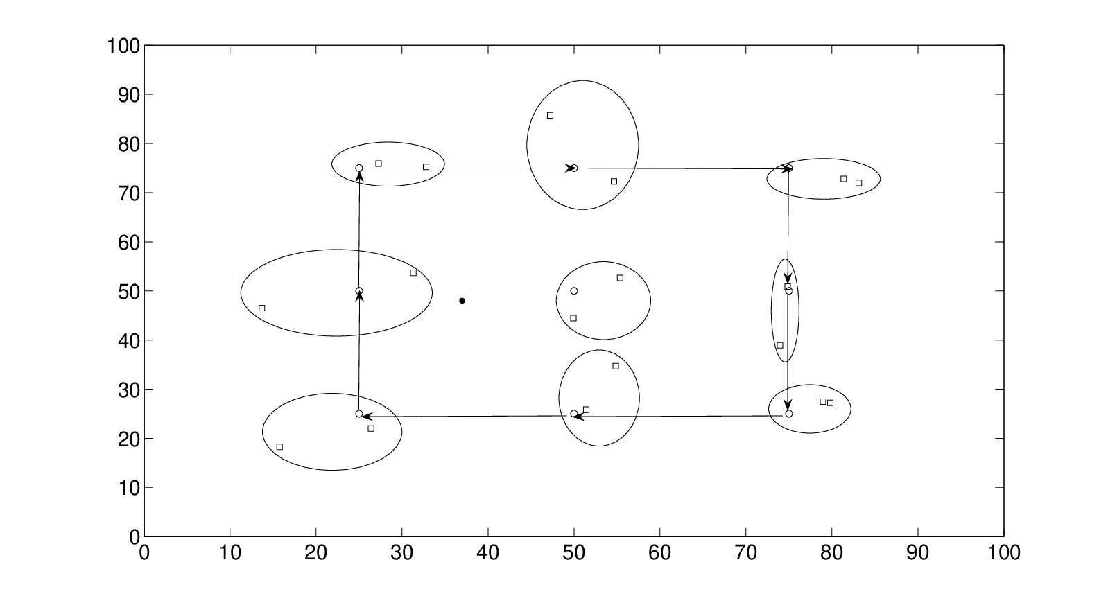
The sampling interval is $10$ time units and the measurement noise variance is set to $0.1.$ In deriving the state-space representation, we use $\bar{n}_{1}=\bar{n}_{2}=15.$ We performed three simulation experiments.

1.

Standard IRPE: 1000 iterations of the IRPE algorithm are used to estimate the source location. As discussed, the IRPE algorithm does not use the information that the sensors observe the same under-lying process through different observation matrices $H_{i}.$
2.

Hybrid IRPE: The network is divided into $9$ clusters of size $3.$ The cluster heads are the sensors on the grid. At the beginning of each slot, a cluster head collects the measurements from the sensors in the cluster. To estimate the sensor location, 1000 iterations of IRPE are run between the cluster heads. In determining the predictor family for each cluster’s observations the information that all the sensors in the cluster observe the same underlying process is used. But, in the inter-cluster processing through the IRPE algorithm this information is not used.
3.

Centralized RPE: All sensors immediately communicate their measurements to a fusion center. In this case the information is completely used. The fusion center runs 1000 iterations.

The results are plotted in Figs. 3 and 4. As expected the centralized RPE performs the best. However, what is interesting to note is that the standard IRPE does not converge to the correct solution but is caught in a local minimum. We also observed this in other simulation runs. However, when the sensors are clustered the iterates converge to the correct location.

IX Conclusions

Linear state-space models arise naturally, or as linear approximations to non-linear state-space models, in many applications. In an inference setting where the aim is to estimate a quantity of interest, it is quite natural for the state-space models to be parametrized by the unknown quantity of interest. In a control system setting where the aim is to control the process, it is common to use such incomplete state-space models as ‘grey-box’ descriptions of the system that is to be controlled. Thus, the problem addressed in this paper is important in both of these settings.

In Section VII we could only give a qualitative description of the tradeoff between centralized and distributed schemes. It is therefore of interest to find good bounds on the performance of the IRPE and RPE schemes that can be used to quantify the loss in performance. Also, to truly understand the performance of the algorithm in practical settings, we need to obtain convergence results when there are communication errors. Further, we have considered a simple class of networks where the topology is fixed. It is important to obtain an algorithm that is similar to the IRPE for networks with a random and time-varying topologies. Finally, as mentioned in Section VII, the result and analysis extend easily to the case where there is an open-loop input to the system. An important extension is to obtain similar convergence results for some common classes of closed-loop inputs using the techniques discussed in Appendix 7.A of [1].

References

[1] L. Ljung and T. Söderström, Theory and Practice of Recursive Identification, The MIT press, 1983.
[2] S. Roweis and Z. Ghahramani, “A unifying review of linear gaussian models,” Neural Computation, vol. 11, 1999.
[3] S. Chen, C. Cowan, S. Billings, and P. Grant, “Parallel recursive prediction error algorithm for training layered neural networks,” International Journal of Control, vol. 51, 1990.
[4] D. Blatt and A. Hero, “Distributed maximum likelihood estimation for sensor networks,” in Proceedings of the IEEE International Conference on Acoustics, Speech and Signal Processing, 2004.
[5] R. D. Nowak, “Distributed EM algorithms for density estimation and clustering in sensor networks,” IEEE Transactions on Signal Processing, vol. 51, 2003.
[6] M. Rabbat and R. Nowak, “Distributed optimization in sensor networks,” in Proceedings of IPSN’04, 2004.
[7] A. Nedić and D. P. Bertsekas, “Incremental subgradient method for nondifferentiable optimization,” SIAM Journal of Optimization, vol. 12, 2001.
[8] L. Xiao, S. Boyd, and S. Lall, “A scheme for robust distributed fusion based on average consensus,” in Proceedings of the International Conference on Information Processing in Sensor Networks, 2005.
[9] S. Sundhar Ram, A. Nedić, and V. V. Veeravalli, “Incremental Robbins-Monro gradient algorithm for regression in sensor networks,” in Proceedings of the Asilomar Conference on Signals, Systems, and Computers, 2007.
[10] C. G. Lopes and A. H. Sayeed, “Incremental adaptive strategies over distributed networks,” IEEE Transactions on Signal Processing, vol. 55, 2007.
[11] H. Poor, An Introduction to Signal Detection and Estimation, Birkäuser, 1994.
[12] P. Kumar and P. Varaiya, Stochastic systems: Estimation, Identification and Adaptive Control, Prentice-Hall, 1986.
[13] D. P. Bertsekas and J. N. Tsitsiklis, “Gradient convergence in gradient methods with errors,” SIAM Journal of Optimization, vol. 10, 2000.
[14] M. V. Solodov, “Incremental gradient algorithms with stepsizes bounded away from zero,” Computational Optimization and Algorithms, vol. 11, 1998.
[15] J. Matthes, L. Gröll, and H. B. Keller, “Source localization for spatially distributed electronic noses for advection and diffusion,” IEEE Transactions on Signal Processing, vol. 53, no. 5, 2005.
[16] T. Zhao and A. Nehorai, “Distributed sequential Bayesian esimation of a diffusive source in wireless sensor networks,” IEEE Transactions on Signal Processing, vol. 55, 2007.
[17] Y. Levinbook and T. F. Wong, “Maximum likelihood diffusive source localization based on binary observations,” in Conference Record of the Thirty-Eighth Asilomar Conference on Signal, Systems and Computers, 2004.
[18] M. E. Alpay and M. H. Shor, “Model-based solution techniques for the source localization problem,” IEEE Transactions on Control Systems Technology, vol. 8, no. 6, 2000.
[19] J. R. Cannon and P. DuChateau, “Structural identification of an unkown source term in a heat equation,” Inverse Problems, vol. 14, 1998.
[20] C. L. Niliot and F. Lefévre, “Multiple transient point heat sources identification in heat diffusion: Application to numerical two- and three-dimensional problems,” Numerical Heat Transfer, vol. 39, 2001.
[21] S. Sundhar Ram and V. V. Veeravalli, “Localization and intensity tracking of a diffusing point source using sensor networks,” in Proceedings of IEEE Globecom, 2007.
[22] L. I. Piterbarg and B. L. Rozovskii, “On asymptotic problems of parameter estimation in stochastic PDE’s: the case of discrete time sampling,” Mathematical Methods of Statistics, vol. 6, 1997.
[23] L. Rossi, B. Krishnamachari, and C. C. J. Kuo, “Distributed parameter estimation for monitoring diffusion phenomena using physical models,” in First IEEE International Conference on Sensor and Ad Hoc Communications and Networks, 2004.

-A Proof of Theorem 2

We take the following approach to prove Theorem 2. First, we consider a centralized system where the sensors immediately communicate all their measurements to a fusion center. For this system we use the RPE algorithm to generate a sequence of iterates, and then we show that this iterate sequence is identical to the iterate sequence generated by the IRPE algorithm. We complete the proof by proving that the iterates converge to a local minimum of $f(x).$

In what follows, we extensively use the notion of block vectors and matrices. For positive integers $a$ and $b,$ let $\mathcal{M}_{a\times b}$ be the vector space of all real matrices of dimensions $a\times b.$ A block vector in $\mathcal{M}_{a\times b}$ is a vector whose elements are from $\mathcal{M}_{a\times b}.$ The length of a block vector is the number of block elements. In a similar manner, block matrices in $\mathcal{M}_{a\times b}$ are matrices where each element is itself a matrix from $\mathcal{M}_{a\times b}$ . While writing block matrices we will allow for a slight abuse of notation and use $0$ and $I$ to denote the zero and identity matrices, respectively. Their dimensions can be unambiguously fixed from the dimensions of the other blocks in the block matrix. We will use $\mbox{\boldmath{$U$}}^{a}_{b},$ $b\leq m,$ to denote the unit block vector in $\mathcal{M}_{a\times a}$ of length $m,$ with the $b$ -th block equal to the identity matrix in $\mathcal{M}_{a\times a}$ and all the other blocks equal to the zero matrix in $\mathcal{M}_{a\times a}.$

We allow $i,j$ to take values in the set $\mathcal{I}=\{1,\ldots,m\}.$ We define $\delta[\cdot]$ as the Kronecker delta. Recall that the dimension of the matrices $\Theta_{i}(k;x)$ is $q,$ the dimension of the measurement $r_{i}(k)$ is $p,$ and the dimension of the parameter vector $x$ is $d.$ Also, recall that for any random process $\{Y(k;x)\}$ that is parametrized by $x,$ $y(k)$ denotes the sample path of $Y(k;x^{*}).$

-A1 State-space model for sensor observations

Without loss of generality, assume that each time slot has duration of $m$ time units. Consider a hypothetical centralized scheme where at time $mk+j,$ sensor $j$ communicates $r_{j}(k+1)$ to the fusion center over a perfect delayless link. For $i\neq j,$ sensor $i$ communicates a predetermined constant value, say $0$ , that does not convey any information about the value taken by the parameter $x.$

Denote the sequence communicated by a sensor $i$ by $\{\bar{r}_{i}(mk+j)\}$ , with

\bar{r}_{i}(mk+j)=r_{i}(k+1)\delta[i-j].

(84)

Next, denote the observation sequence at the fusion center by $\{\tilde{r}(mk+j)\}$ , where

\tilde{r}(mk+j)=\left[\bar{r}_{1}(mk+j)\,\ldots\,\bar{r}_{m}(mk+j)\right]^{T}=\mbox{\boldmath{$U$}}^{p}_{j}r_{j}(k+1).

(85)

We now consider the problem of estimating $x$ from observation sequence $\{\tilde{r}(mk+j)\}.$ We show that the random process $\tilde{R}(mk+j;x)$ can be represented as the output vector of a suitably defined state-space system. For this, we first use the relations in (2) to obtain the equations describing the evolution $\{\bar{R}_{i}(mk+j;x)\}.$ Note that from (84), we have

\bar{R}_{i}(mk+j;x)=R_{i}(k+1;x)\ \delta[i-j].

(86)

Let $\bar{D}_{i}(x)$ be the following $m\times m$ block matrix in $\mathcal{M}_{q\times q}$ :

\displaystyle\bar{D}_{i}(x)=\left[\begin{array}[]{cccccc}0&I&0&\cdot&\cdot&0\\ 0&0&I&\cdot&\cdot&0\\ \cdot&\cdot&\cdot&\cdot&\cdot&\cdot\\ 0&0&0&\cdot&\cdot&I\\ D_{i}(x)&0&0&\cdot&\cdot&0\end{array}\right].

Observe that

\displaystyle\bar{D}_{i}(x)\mbox{\boldmath{$U$}}^{q}_{j}=\begin{cases}\mbox{\boldmath{$U$}}^{q}_{j-1}&\mbox{ when $j\neq 1$}\\ \mbox{\boldmath{$U$}}^{q}_{m}\ D_{i}(x)&\mbox{ when $j=1$}.\end{cases}

(92)

Also, define $\bar{H}_{i}=H_{i}\,\left(\mbox{\boldmath{$U$}}^{q}_{1}\right)^{T},$ and note that

\displaystyle\bar{H}_{i}\mbox{\boldmath{$U$}}^{q}_{j}=H_{i}\ \left(\mbox{\boldmath{$U$}}^{q}_{1}\right)^{T}\mbox{\boldmath{$U$}}^{q}_{j}=H_{i}\delta[j-1].

(93)

Define $\bar{\Theta}_{i}(0;x)=\mbox{\boldmath{$U$}}^{q}_{i}\ \Theta_{i}(0;x),$ and

		$\displaystyle\bar{\Theta}_{i}(mk+j;x)=\begin{cases}\mbox{\boldmath{$U$}}^{q}_{i-j+1}\ \Theta_{i}(k+1;x)\ \ \ &\mbox{ if $j\leq i$}\\ \mbox{\boldmath{$U$}}^{q}_{m+1-(j-i)}\ \Theta_{i}(k+2;x)&\mbox{ if $j>i$,}\end{cases}$		(94)
		$\displaystyle\bar{W}_{i}(mk+j;x)=\mbox{\boldmath{$U$}}^{q}_{m}\ W_{i}(k+1;x)\ \delta[i-j],$
		$\displaystyle\bar{V}_{i}(mk+j)=V_{i}(k+1)\ \delta[i-j].$		(95)

The following is an illustration for $\bar{\Theta}_{i}(mk+j;x)$ with $i=3$ and $j=2,3,4$ :

\begin{array}[]{ccc}mk+2&mk+3&mk+4\\ \\ \left[\begin{array}[]{c}0\\ \Theta_{3}(k+1;x)\\ 0\\ \vdots\\ 0\\ 0\end{array}\right]&\left[\begin{array}[]{c}\Theta_{3}(k+1;x)\\ 0\\ 0\\ \vdots\\ 0\\ 0\end{array}\right]&\left[\begin{array}[]{c}0\\ 0\\ 0\\ \vdots\\ 0\\ \Theta_{3}(k+2;x)\end{array}\right].\end{array}

Claim 1

For all $n\geq 0,$ we have

	$\displaystyle\bar{\Theta}_{i}(n+1;x)$	$\displaystyle=\bar{D}_{i}(x)\bar{\Theta}_{i}(n;x)+\bar{W}_{i}(n;x),$		(96)
	$\displaystyle\bar{R}_{i}(n+1;x)$	$\displaystyle=\bar{H}_{i}\bar{\Theta}_{i}(n+1;x)+\bar{V}_{i}(n+1).$		(97)

Proof:

Let $n=mk+j.$ Substitute for $\bar{\Theta}_{i}(n;x)$ and $\bar{W}_{i}(n;x)$ from (94) in the right hand side (RHS) of (96). For $i<j,$ from (92) we obtain

	RHS of (96)	$\displaystyle=\bar{D}_{i}(x)\mbox{\boldmath{$U$}}^{q}_{i-j+1}\ \Theta_{i}(k+1;x)+0$
		$\displaystyle=\mbox{\boldmath{$U$}}^{q}_{i-j}\Theta_{i}(k+1;x)$
		$\displaystyle=\mbox{\boldmath{$U$}}^{q}_{i-(j+1)-1}\Theta_{i}(k+1;x)$
		$\displaystyle=\bar{\Theta}_{i}(mk+j+1;x).$

For $i=j,$ using (92) and (2), we obtain

	RHS of (96)	$\displaystyle=\bar{D}_{i}(x)\mbox{\boldmath{$U$}}^{q}_{1}\ \Theta_{i}(k+1;x)+\mbox{\boldmath{$U$}}^{q}_{m}\ W_{i}(k+1;x)$
		$\displaystyle=\mbox{\boldmath{$U$}}^{q}_{m}D_{i}(x)\Theta_{i}(k+1;x)+\mbox{\boldmath{$U$}}^{q}_{m}\ W_{i}(k+1;x)$
		$\displaystyle=\mbox{\boldmath{$U$}}^{q}_{m}(D_{i}(x)\Theta_{i}(k+1;x)+W_{i}(k+1;x))$
		$\displaystyle=\mbox{\boldmath{$U$}}^{q}_{m}\Theta_{i}(k+2;x)$
		$\displaystyle=\bar{\Theta}_{i}(mk+j+1;x).$

Finally, when $i<j,$ from (92) we have

	RHS of (96)	$\displaystyle=\bar{D}_{i}(x)\mbox{\boldmath{$U$}}^{q}_{m-(j-i)+1}\ \Theta_{i}(k+2;x)+0$
		$\displaystyle=\mbox{\boldmath{$U$}}^{q}_{m-(j-i)}\Theta_{i}(k+2;x)$
		$\displaystyle=\mbox{\boldmath{$U$}}^{q}_{m-(j+1-i)-1}\Theta_{i}(k+2;x)$
		$\displaystyle=\bar{\Theta}_{i}(mk+j+1;x),$

thus, completing the proof of the relation in (96).

We next prove the relation in (97). At first, we consider the case when $j\neq m$ and show that the following relation holds:

\bar{H}_{i}\bar{\Theta}_{i}(mk+j+1;x)+\bar{V}_{i}(mk+j+1)=R_{i}(k+1)\delta[i-j-1].

Let $i\neq j+1,$ and note that from (95) we have $\bar{V}_{i}(n+1)=0.$ Furthermore, from the definition of $\bar{\Theta}_{i}(n;x)$ in (94) we obtain

\bar{H}_{i}\bar{\Theta}_{i}(mk+(j+1);x)=\begin{cases}\mbox{\boldmath{$U$}}^{q}_{i-j}\Theta_{i}(k+1;x)&\mbox{ $i>j+1$}\\ \mbox{\boldmath{$U$}}^{q}_{m-(j-i)}\Theta_{i}(k+2;x)&\mbox{ $i<j+1$}\end{cases}

Using the expression in (93), we can immediately verify that $\bar{H}_{i}\bar{\Theta}_{i}(mk+(j+1);x)=0.$ Therefore, we have $\bar{R}_{i}(n+1;x)=0$ for $i\neq j+1.$

When $i=j+1,$ $\bar{V}_{i}(mk+j+1)=V_{j+1}(k+1)$ and

\bar{H}_{j+1}\bar{\Theta}_{i}(mk+j+1;x)=\bar{H}_{j+1}\mbox{\boldmath{$U$}}^{q}_{1}=H_{j+1}\Theta_{j+1}(k+1;x).

Therefore, from (2) we see that $\bar{R}_{i}(mk+j+1;x)=R_{i}(k+1;x)$ for $i=j+1,$ thus, concluding the proof of relation (97) for $j\neq m.$

When $j=m,$ by using arguments similar to that of the preceding case $j\neq m,$ we can show that

\bar{H}_{i}\bar{\Theta}_{i}(mk+j+1;x)+\bar{V}_{i}(mk+j+1)=R_{1}(k+2)\delta[i-1],

thus, completing the proof. ∎

Now, by combining the equations in (96)–(97) for $i\in\mathcal{I},$ we provide evolution equations for $\{\tilde{R}(n;x)\}.$ Define

		$\displaystyle\tilde{F}(x)=\mbox{diag}\left(\bar{F}_{1}(x),\ldots,\bar{F}_{m}(x)\right),$
		$\displaystyle\tilde{H}(x)=\mbox{diag}\left(\bar{H}_{1}(x),\ldots,\bar{H}_{m}(x)\right),$
		$\displaystyle\tilde{\Theta}(n;x)=\left[\begin{array}[]{c}\bar{\Theta}_{1}(n;x)\\ \vdots\\ \bar{\Theta}_{m}(n;x)\end{array}\right],\ \ \tilde{W}(n;x)=\left[\begin{array}[]{c}\bar{W}_{1}(n;x)\\ \vdots\\ \bar{W}_{m}(n;x)\end{array}\right],\ \ \tilde{V}(n;x)=\left[\begin{array}[]{c}\bar{V}_{1}(n;x)\\ \vdots\\ \bar{V}_{m}(n;x)\end{array}\right].$

Using the relations in (96) and (97), we can write

	$\displaystyle\tilde{\Theta}(n+1;x)$	$\displaystyle=\tilde{D}(x)\tilde{\Theta}(n;x)+\tilde{W}(n;x),$		(107)
	$\displaystyle\tilde{R}(n+1;x)$	$\displaystyle=\tilde{H}\tilde{\Theta}_{i}(n+1;x)+\tilde{V}(n+1).$		(108)

To apply the RPE we need to determine a predictor family for $\tilde{R}(n;x^{*})$ that is parametrized by $x$ and is asymptotically optimal at $x=x^{*}.$ We do this in the next section.

-A2 Time-Invariant Kalman Predictor for Centralized System

Let us first obtain the time-invariant Kalman predictor for $\bar{R}_{i}(n;x)$ . Fix $n=mk+j$ and define

	$\displaystyle\bar{\phi}_{i,n}(x;\bar{r}_{i}^{n-1})$	$\displaystyle=\begin{cases}\mbox{\boldmath{$U$}}^{q}_{i-j+1}\ \phi_{i,k+1}(x;r_{i}^{k})\ \ \ &\mbox{ if $j\leq i$}\\ \mbox{\boldmath{$U$}}^{q}_{m+1-(j-i)}\ \phi_{i,k+2}(x;r_{i}^{k+1})&\mbox{ if $j>i$,}\end{cases}$		(109)
		$\displaystyle\bar{g}_{i,n}(x;\bar{r}_{i}^{n-1})=g_{i,k+1}(x;r_{i}^{k})\ \delta[j-i].$		(110)

Note that $\phi_{i,k+1}(x^{*};r_{i}^{k})$ and $g_{i,k+1}(x^{*};r_{i}^{k}),$ are the time-invariant Kalman predictors for $\Theta_{i}(k+1;x^{*})$ and $R_{i}(k+1;x^{*}),$ respectively. Therefore, from (94) we can conclude that $\bar{\phi}_{i,n}(x^{*};\bar{r}_{i}^{n-1})),$ resp. $\bar{g}_{i,n}(x^{*};\bar{r}_{i}^{n-1}),$ is asymptotically optimal for $\bar{\Theta}_{i}(n;x^{*}),$ resp. $\bar{R}_{i}(n;x^{*})$ .

Define

\displaystyle\bar{G}_{i}(x)=\mbox{\boldmath{$U$}}^{p}_{m}\ G_{i}(x),

(111)

and $\bar{F}_{i}(x)=\bar{D}_{i}(x)-\bar{G}_{i}(x)\bar{H}_{i}.$ The matrix $\bar{F}_{i}(x)$ will have the same form as $\bar{D}_{i}(x)$ in (-A1) but with $D_{i}(x)$ replaced by $F_{i}(x).$ Similar to Claim 1, we can show that

	$\displaystyle\bar{\phi}_{i,n+1}(x;\bar{r}_{i}^{n})$	$\displaystyle=\bar{F}_{i}(x)\bar{\phi}_{i,n}(x;\bar{r}_{i}^{n-1})+\bar{G}_{i}(x)\bar{r}_{i}(n),$
	$\displaystyle\bar{g}_{i,n+1}(x;\bar{r}_{i}^{n})$	$\displaystyle=\bar{H}_{i}(x)\bar{\phi}_{i,n}(x;\bar{r}_{i}^{n}).$		(112)

We can immediately obtain a predictor family for $\tilde{\Theta}(n;x^{*})$ and $\{\tilde{R}_{n}(x^{*})\}$ that is asymptotically optimal at $x=x^{*}$ as follows:

	$\displaystyle\tilde{\phi}_{n}(x;\tilde{r}^{n-1})$	$\displaystyle=\left[\bar{\phi}_{1,n}(x;\bar{r}_{1}^{n-1})\ldots\bar{\phi}_{m,n}(x;\bar{r}_{m}^{n-1})\right]^{T},$
	$\displaystyle\tilde{g}_{n}(x;\tilde{r}^{n-1})$	$\displaystyle=\left[\bar{g}_{1,n}(x;\bar{r}_{1}^{n-1})\ldots\bar{g}_{m,n}(x;\bar{r}_{m}^{n-1})\right]^{T}.$

Furthermore, from (112) one can verify that

	$\displaystyle\tilde{\phi}_{n+1}(x;\tilde{r}^{n})$	$\displaystyle=\tilde{F}(x)\tilde{\phi}_{n}(x;\tilde{r}^{n-1})+\tilde{G}(x)\tilde{r}(n),$
	$\displaystyle\tilde{g}_{n+1}(x;\tilde{r}^{n})$	$\displaystyle=\tilde{H}\phi_{n+1}(x;\tilde{r}^{n}),$		(113)

where

\tilde{G}(x)=\mbox{diag}\left(\bar{G}_{1}(x),\ldots,\bar{G}_{m}(x)\right).

(114)

-A3 RPE Algorithm for Centralized System

Here, we use the RPE algorithm to estimate $x$ from $\{\tilde{r}(n)\}.$ As we mentioned earlier, $\tilde{r}(n)$ contans the same information as $\hat{r}(n)$ about the true value of $x$ . Define for $\ell=1,\ldots,d,$

\nabla^{(\ell)}\tilde{F}(x)=\frac{\partial\tilde{F}(x)}{\partial x^{(\ell)}},\qquad\nabla^{(\ell)}G(x)=\frac{\partial\tilde{G}(x)}{\partial x^{(\ell)}}.

We define the iterates $\{\tilde{x}_{n}\}$ as follows:

$\displaystyle\left[\begin{array}[]{c}\tilde{h}_{n+1}\\ \tilde{\xi}^{(\ell)}_{n+1}\end{array}\right]$	$\displaystyle=$	$\displaystyle\left[\begin{array}[]{cc}\tilde{H}&0\\ 0&\tilde{H}\end{array}\right]\left[\begin{array}[]{c}\tilde{\psi}_{n+1}\\ \tilde{\chi}^{(\ell)}_{n+1}\end{array}\right],$
$\displaystyle\tilde{\epsilon}_{n+1}$	$\displaystyle=$	$\displaystyle\tilde{r}(n+1)-\tilde{h}_{n+1},$	(122)
$\displaystyle\underline{\tilde{x}}^{(\ell)}_{n+1}$	$\displaystyle=$	$\displaystyle\tilde{x}^{(\ell)}_{n}-\tilde{\alpha}_{n+1}\ \left(\tilde{\xi}^{(\ell)}_{n+1}\right)^{T}\,\tilde{\epsilon}_{n+1},$	(123)
$\displaystyle\underline{\tilde{x}}_{n+1}$	$\displaystyle=$	$\displaystyle\left[\underline{\tilde{x}}^{(1)}_{n+1}\,\ldots\,\underline{\tilde{x}}^{(d)}_{n+1}\right]^{T},$	(124)
$\displaystyle\tilde{x}_{n+1}$	$\displaystyle=$	$\displaystyle\mathcal{P}_{X}\left[\underline{\tilde{x}}_{n+1}\right],$	(125)
$\displaystyle\left[\begin{array}[]{c}\tilde{\psi}_{n+2}\\ \tilde{\chi}^{(\ell)}_{n+2}\end{array}\right]$	$\displaystyle=$	$\displaystyle\left[\begin{array}[]{cc}\tilde{F}(\tilde{x}_{n+1})&0\\ \nabla^{(\ell)}\tilde{F}(\tilde{x}_{n+1})&\tilde{F}(\tilde{x}_{n+1})\end{array}\right]\left[\begin{array}[]{c}\tilde{\psi}_{n+1}\\ \tilde{\chi}^{(\ell)}_{n+1}\end{array}\right]+\left[\begin{array}[]{c}\tilde{G}(\tilde{x}_{n+1})\\ \nabla^{(\ell)}G(\tilde{x}_{n+1})\end{array}\right]\tilde{r}(n+1).$

Here, $\alpha(n)=\alpha_{k+1}$ for $n=mk+j$ for $j=1,\ldots,m-1.$ Next, we assign the initial values for the recursion. Recall that the IRPE algorithm in (VI) is initialized with the values $\psi_{i,1}=\psi_{i,s},$ $\xi^{(\ell)}_{i,1}=\xi^{(\ell)}_{i,s}$ for all $i$ and $\ell$ , and $x_{0}=x_{s}.$ We let $\tilde{x}_{0}=x_{s},$ and

\displaystyle\tilde{\psi}_{0}=\left[\begin{array}[]{c}\bar{\psi}_{1,s}\\ \vdots\\ \bar{\psi}_{m,s}\end{array}\right],\ \ \ \tilde{\xi}^{(\ell)}_{0}=\left[\begin{array}[]{c}\bar{\xi}^{(\ell)}_{1,s}\\ \vdots\\ \bar{\xi}^{(\ell)}_{m,s}\end{array}\right],

where $\bar{\psi}_{i,s}=\mbox{\boldmath{$U$}}^{q}_{i}\psi_{i,s}$ and $\bar{\xi}^{(\ell)}_{i,s}=\mbox{\boldmath{$U$}}^{q}_{i}\xi^{(\ell)}_{i,s}$ for all $i$ and $l.$

-A4 Rest of the proof

Finally, here we show that $\tilde{x}_{n}=z_{j,k+1}.$ Recall that $\psi_{i,k}$ and $\chi^{(\ell)}_{i,k}$ are generated in the IRPE algorithm (VI)–(VI). Define for $l=1,\ldots,d,$

	$\displaystyle\bar{\psi}_{i,n}$	$\displaystyle=\begin{cases}\mbox{\boldmath{$U$}}^{q}_{i-j+1}\ \psi_{i,k+1}\ \ \ &\mbox{ if $j\leq i$}\\ \mbox{\boldmath{$U$}}^{q}_{m+1-(j-i)}\ \psi_{i,k+2}&\mbox{ if $j>i$,}\end{cases}$		(141)
	$\displaystyle\bar{\chi}^{(\ell)}_{i,n}$	$\displaystyle=\begin{cases}\mbox{\boldmath{$U$}}^{q}_{i-j+1}\ \chi^{(\ell)}_{i,k+1}\ \ \ &\mbox{ if $j\leq i$}\\ \mbox{\boldmath{$U$}}^{q}_{m+1-(j-i)}\ \chi^{(\ell)}_{i,k+2}&\mbox{ if $j>i$.}\end{cases}$		(142)

We next establish the following lemma. Once we prove this lemma we can use induction to show that the iterates generated by the IRPE algorithm are the same as those generated by the centralized scheme.

Lemma 1

Let $n=mk+j.$ If $\tilde{x}_{n}=z_{j,k+1}$ and

	$\displaystyle\tilde{\psi}_{n+1}$	$\displaystyle=\left[\bar{\psi}_{1,n+1}\,\ldots\,\bar{\psi}_{m,n+1}\right]^{T},$		(143)
	$\displaystyle\tilde{\chi}^{(\ell)}_{n+1}$	$\displaystyle=\left[\bar{\chi}^{(\ell)}_{1,n+1}\,\ldots\,\bar{\chi}^{(\ell)}_{m,n+1}\right]^{T}\qquad{{\hbox{for }\ell=1,\ldots,d,}}$		(144)

then $\tilde{x}_{n}=z_{j+1,k+1},$ and

	$\displaystyle\tilde{\psi}_{n+2}$	$\displaystyle=\left[\bar{\psi}_{1,n+2}\,\ldots\,\bar{\psi}_{m,n+2}\right]^{T},$
	$\displaystyle\tilde{\chi}^{(\ell)}_{n+2}$	$\displaystyle=\left[\bar{\chi}^{(\ell)}_{1,n+2}\,\ldots\,\bar{\chi}^{(\ell)}_{m,n+2}\right]^{T}\qquad{{\hbox{for }\ell=1,\ldots,d.}}$

Proof:

For a block vector $A,$ let $A^{(i)}$ denote its $i$ -th block. Substituting for $\tilde{\psi}_{mk+j+1}$ from (143) in (-A3), and noting from (-A1) that $\tilde{H}$ is a block diagonal matrix with the $(i,i)$ -th block equal to $\bar{H}_{i}$ , we can see that

\displaystyle\tilde{h}_{mk+j+1}^{(i)}

\displaystyle=(\tilde{H}\tilde{\psi}_{mk+j+1})^{(i)}=\bar{H}_{i}\bar{\psi}_{i,mk+j+1}.

Using the definition of $\bar{\psi}_{i,mk+j+1}$ from (141) and noting from (93) that $\bar{H}_{i}\mbox{\boldmath{$U$}}^{q}_{j}=H_{i}\delta[j-1]$ , we obtain

	$\displaystyle\tilde{h}^{(i)}_{mk+(j+1)}$	$\displaystyle=\bar{H}_{i}\bar{\psi}_{i,mk+(j+1)}$
		$\displaystyle=\begin{cases}\bar{H}_{i}{{U}}^{q}_{i-(j+1)-1}\psi_{i,k+1}&\mbox{ if $i>j+1$}\\ \bar{H}_{i}{{U}}^{q}_{1}\psi_{i,k+1}&\mbox{ if $i=j+1$}\\ \bar{H}_{i}{{U}}^{q}_{m-(j+1-i)+1}\psi_{i,k+1}&\mbox{ if $i<j+1$}\end{cases}$
		$\displaystyle=\begin{cases}0&\mbox{ if $i\neq j+1$}\\ H_{j+1}\psi_{j+1,k+1}&\mbox{ if $i=j+1$}.\end{cases}$

Using (VI) we replace $H_{j+1}\psi_{j+1,k+1}$ by $h_{j+1,k+1}$ and write

\displaystyle\tilde{h}^{(i)}_{mk+(j+1)}=h_{i,k+1}\delta[i-j-1].

Therefore, $\tilde{h}_{mk+j+1}=\mbox{\boldmath{$U$}}^{{{p}}}_{j+1}\ h_{j+1,k+1}.$ Similarly, we can see that for all $\ell$ ,

\displaystyle\tilde{\xi}^{(\ell)}_{mk+j+1}=\mbox{\boldmath{$U$}}^{p}_{j+1}\ \xi^{(\ell)}_{j+1,k+1}.

(145)

Substituting in (122) for $\tilde{h}_{mk+j+1}$ from above and for $\tilde{r}_{mk+j+1}$ from (85) we get

\displaystyle\tilde{\epsilon}_{mk+j+1}=\mbox{\boldmath{$U$}}^{p}_{j+1}(h_{j+1,k+1}-r_{j+1}(k+1)).

Observe that $\epsilon_{j+1,k+1}=h_{j+1,k+1}-r_{j+1}(k+1)$ from (66), so that

\displaystyle\tilde{\epsilon}_{mk+j+1}=\mbox{\boldmath{$U$}}^{p}_{j+1}\epsilon_{j+1,k+1}.

(146)

Since $\tilde{x}_{mk+j}=z_{j,k+1}$ it follows that $\tilde{x}^{{{(l)}}}_{mk+j}=z^{(\ell)}_{j,k+1}.$ Substituting from (145) and (146) in (123) we get for all $\ell$ ,

	$\displaystyle\underline{\tilde{x}}^{(l)}_{mk+j+1}$	$\displaystyle=z^{(\ell)}_{j,k+1}-\alpha_{k+1}\left(\mbox{\boldmath{$U$}}^{p}_{j+1}\xi^{(\ell)}_{j+1,k+1}\right)^{T}\mbox{\boldmath{$U$}}^{p}_{j+1}\epsilon_{j+1,k+1}$
		$\displaystyle=z^{(\ell)}_{j,k+1}-\alpha_{k+1}\left(\xi^{(\ell)}_{j+1,k+1}\right)^{T}\epsilon_{j+1,k+1}$
		$\displaystyle=\underline{z}^{(\ell)}_{j+1,k+1}.$

The last step follows from (67). Therefore, from (124) and (68) we can conclude that $\underline{\tilde{x}}_{mk+j+1}=\underline{z}_{j+1,k+1}$ and from (125) and (69) that $\tilde{x}_{mk+j+1}=z_{j+1,k+1}.$ This completes the first part of the proof.

Let us next consider the case when $j\in\{1,\ldots,m-1\}.$ In (-A3) let us replace $\tilde{x}_{n+1}$ with $z_{j+1,k+1}.$ Note from (-A1), respectively (114), that $\tilde{F}(z_{j+1,k+1}),$ respectively $\tilde{G}(z_{j+1,k+1}),$ is a block diagonal matrix with $(i,i)$ -th block equal to $\bar{F}_{i}(z_{j+1,k+1}),$ respectively $\bar{G}_{i}(z_{j+1,k+1}).$ Substituting for $\tilde{\psi}_{n+1}$ from (143) and $\tilde{r}(n+1)$ from (85) in (-A3) we can write

\displaystyle\tilde{\psi}^{(i)}_{mk+j+2}=

\displaystyle\bar{F}_{i}(z_{j+1,k+1})\bar{\psi}_{i,mk+j+1}+\bar{G}_{i}(z_{j+1,k+1})\bar{r}_{i}(mk+j+1).

Let us substitute for $\bar{G}_{i}(z_{j+1,k+1})$ from (114), for $\bar{\psi}_{i,mk+j+1}$ from (141) and for $\bar{r}_{i}(mk+j+1)$ from (84). Using (92) we get for $i>j+1,$

	$\displaystyle\tilde{\psi}^{(i)}_{mk+j+2}$	$\displaystyle=\bar{F}_{i}(z_{i,k+1})\mbox{\boldmath{$U$}}^{q}_{i-j}\psi_{i,k+1}+0$
		$\displaystyle=\mbox{\boldmath{$U$}}^{q}_{i-j-1}\psi_{i,k+1}$
		$\displaystyle=\bar{\psi}_{i,mk+j+2}.$

When $i=j+1,$ from (VI) we obtain

	$\displaystyle\tilde{\psi}^{(i)}_{mk+j+2}$	$\displaystyle=\bar{F}_{i}(z_{i,k+1})\mbox{\boldmath{$U$}}^{q}_{1}\psi_{j+1,k+1}+\bar{G}_{i}(z_{j+1,k+1})\bar{r}_{i}(n+1)$
		$\displaystyle=\mbox{\boldmath{$U$}}^{q}_{m}F_{i}(z_{i,k+1})\psi_{i,k+1}+\mbox{\boldmath{$U$}}^{q}_{m}G_{i}(z_{i,k+1})r_{i}(k+1)$
		$\displaystyle=\mbox{\boldmath{$U$}}^{q}_{m}\psi_{i,k+2}$
		$\displaystyle=\bar{\psi}_{i,mk+j+2}.$

When $i<j+1,$ we have

	$\displaystyle\tilde{\psi}^{(i)}_{mk+j+2}$	$\displaystyle=\bar{F}_{i}(z_{i,k+1})\mbox{\boldmath{$U$}}^{q}_{m-(j-i)}\psi_{i,k+2}+0$
		$\displaystyle=\mbox{\boldmath{$U$}}^{q}_{m-(j-i)-1}\psi_{i,k+2}$
		$\displaystyle=\bar{\psi}_{i,mk+j+2}.$

Equation (143) can be shown similarly for the case $j=m.$ The proof of relation (144) is very similar to that of relation (143) and therefore, it is omitted. ∎

Observe that the initial values for the RPE algorithm in (-A3) and the IRPE algorithm in (VI) are choosen such that $\tilde{x}_{0}=z_{0,1},$ and

	$\displaystyle\tilde{\psi}_{1}$	$\displaystyle=\left[\bar{\psi}_{1,1}\,\ldots\,\bar{\psi}_{m,1}\right]^{T},$
	$\displaystyle\tilde{\chi}^{(\ell)}_{1}$	$\displaystyle=\left[\bar{\chi}^{(\ell)}_{1,1}\,\ldots\,\bar{\chi}^{(\ell)}_{m,1}\right]^{T}\quad{{\hbox{for all $\ell$}.}}$

By using Lemma 1 and the induction on $k$ , we can conclude that $\tilde{x}_{mk+i}=z_{i,k+1}$ for all $k\geq 1$ and $i\in\mathcal{I}$ . To complete the proof, we only need to show that the sequence $\{\tilde{x}_{n}\}$ converges to a minimum of $f(x),$ which is done in the following.

Lemma 2

The sequence $\{\tilde{x}_{n}\}$ generated by (-A3)–(-A3) converges to a local minimum of the function $f(x),$ defined in (58), over the set $X$ w.p.1.

Proof:

By the assumptions of Theorem 2, it follows that the conditions of Theorem 1 are satisfied. Therefore, by Theorem 1, the iterates $\tilde{x}_{n}$ converge to a local minimum over the set $X$ of the following function

	$\displaystyle\tilde{f}(x)$	$\displaystyle=\lim_{N\to\infty}\frac{1}{N}\sum_{n=1}^{N}\mathsf{E}\!\left[\left\\|\tilde{R}(n;x^{})-\tilde{g}_{n}(x,\tilde{R}^{n}(x^{}))\right\\|^{2}\right]$
		$\displaystyle=\lim_{N\to\infty}\frac{1}{N}\sum_{n=1}^{N}\sum_{i=1}^{m}\mathsf{E}\!\left[\left\\|\bar{R}_{i}(n;x^{})-\bar{g}_{i,n}(x,\bar{R}_{i}^{n}(x^{}))\right\\|^{2}\right]$
		$\displaystyle=\lim_{N\to\infty}\frac{1}{N}\sum_{n=1}^{N}\sum_{i=1}^{m}\mathsf{E}\!\left[\left\\|R_{i}(n;x^{})-g_{i,n}(x;R_{{{i}}}^{n}(x^{}))\right\\|^{2}\right]$
		$\displaystyle=f(x).$

∎

-B State-space Model for the Sensor Measurements

A standard technique to solve partial differential equations with boundary and initial conditions is to use Green’s function. For the equation in (83) the solution can be written as follows

C(y,t;x)=\int_{0}^{t}\int_{D}I(\tau)\bar{\delta}(z-x)G_{f}(y,z,t-\tau)dz\ d\tau.

Here, $\tau$ and $z=(z_{1},z_{2})$ are parameters of integration, and $G_{f}$ is the following Green’s function

\displaystyle G_{f}(y,z,t)

\displaystyle=\frac{1}{l_{1}l_{2}}+\sum_{n_{1},n_{2}=1}^{\infty}\ \prod_{i=1}^{2}\frac{2}{l_{i}}\exp\left(-\frac{\nu n_{i}^{2}\pi^{2}t}{l_{i}^{2}}\right)\cos\left(\frac{n_{i}\pi y_{i}}{l_{i}}\right)\cos\left(\frac{n_{i}\pi z_{i}}{l_{i}}\right).

Evaluating $C(y,t;x),$ we obtain

\displaystyle C(y,t;x)=\frac{1}{l_{1}l_{2}}\int_{0}^{t}I(\tau)\ d\tau+\sum_{n_{1}=1}^{\infty}\sum_{n_{2}=1}^{\infty}\prod_{i=1}^{2}\left(\frac{2}{l_{i}}\cos\left(\frac{n_{i}\pi y_{i}}{l_{i}}\right)\cos\left(\frac{n_{i}\pi x_{i}}{l_{i}}\right)\right)\left(\int_{0}^{t}I(\tau)\beta_{n_{1},n_{2}}^{t-\tau}\ d\tau\right),

(147)

where

\beta_{n_{1},n_{2}}=\exp\left(-\nu\pi^{2}\sum_{i=1}^{2}\frac{n_{i}^{2}}{l_{i}^{2}}\right).

To get a convenient approximation we will use a sufficiently large, but fixed number of terms in the convergent infinite series in (147). We will let $n_{i},$ $i=1,2,$ vary from $1$ to $\bar{n}_{i},$ where the integers $\bar{n}_{i}>0$ are chosen large enough to provide a sufficiently good approximation. Therefore,

\displaystyle C(y,t;x)\simeq\frac{1}{l_{1}l_{2}}\int_{0}^{t}I(\tau)\ d\tau+\sum_{n_{1}=1}^{\bar{n}_{1}}\sum_{n_{2}=1}^{\bar{n}_{2}}\prod_{i=1}^{2}\left(\frac{2}{l_{i}}\cos\left(\frac{n_{i}\pi y_{i}}{l_{i}}\right)\cos\left(\frac{n_{i}\pi x_{i}}{l_{i}}\right)\right)\left(\int_{0}^{t}I(\tau)\beta_{n_{1},n_{2}}^{t-\tau}\ d\tau\right).

(148)

Define

		$\displaystyle\Theta^{\prime}_{0}(t)=\frac{1}{l_{1}l_{2}}\int_{0}^{t}I(\tau)\ d\tau,$
		$\displaystyle P(y,n_{1},n_{2})=\prod_{i=1}^{2}\cos\left(\frac{n_{i}\pi y_{i}}{l_{i}}\right),$
		$\displaystyle A^{\prime}(x,n_{1},n_{2})=\prod_{i=1}^{2}\cos\left(\frac{n_{i}\pi x_{i}}{l_{i}}\right),$
		$\displaystyle\Theta^{\prime}_{n_{1},n_{2}}(t;x)=A^{\prime}(x,n_{1},n_{2})\left(\int_{0}^{t}I(\tau)\beta_{n_{1},n_{2}}^{t-\tau}\ d\tau\right).$

With this notation we can write (148) as

\displaystyle C(y,t;x)=\Theta^{\prime}_{0}(t)+\sum_{n_{1}=1}^{\bar{n}_{1}}\sum_{n_{2}=1}^{\bar{n}_{2}}\Theta^{\prime}_{n_{1},n_{2}}(t;x)P(y,n_{1},n_{2}).

(149)

From the function $I(t)$ in (81), we have

	$\displaystyle\Theta^{\prime}_{0}(k+1)=$	$\displaystyle\Theta^{\prime}_{0}(k)+I(k+1),$
	$\displaystyle\Theta^{\prime}_{{{n_{1},n_{2}}}}(k+1;x)=$	$\displaystyle\beta_{n_{1},n_{2}}\Theta^{\prime}_{{{n_{1},n_{2}}}}(k;x)+A^{\prime}(x,n_{1},n_{2})I(k+1)\frac{\left(\beta_{n_{1},n_{2}}-1\right)}{\log(\beta_{n_{1},n_{2}})}.$

Furthermore, define

\gamma_{n_{1},n_{2}}=1+n_{2}(n_{1}-1)+n_{2}.

From (148) and (149) we can write $C(y,k+1;x)$ as the output of the following state-space system:

	$\displaystyle\Theta^{\prime}(k+1;x)=$	$\displaystyle D^{\prime}\Theta^{\prime}(k;x)+B^{\prime}(x)I(k+1)$
	$\displaystyle C(y,k+1;x)=$	$\displaystyle H^{\prime}(y)\Theta^{\prime}(k+1;x),$		(150)

where

\displaystyle\Theta^{\prime}_{k+1}=

\displaystyle\left[\theta_{0}(k+1)\,\theta_{1,1}(k+1)\,\ldots\,\theta_{1,\bar{n}_{2}}(k+1)\,\theta_{2,1}(k+1)\,\ldots\,\theta_{\bar{n}_{1},\bar{n}_{2}}(k+1)\right]^{T},

$D^{\prime}$ is the diagonal matrix with

\displaystyle D^{\prime}(1,1)=1,\ \ \ D^{\prime}(\gamma_{n_{1},n_{2}},\gamma_{n_{1},n_{2}})=\beta^{m}_{n_{1},n_{2}},

$B^{\prime}(x)$ is the column vector

	$\displaystyle B^{\prime}(x)\,(1,1)$	$\displaystyle=1$
	$\displaystyle B^{\prime}(x)\,(\gamma_{n_{1},n_{2}},1)$	$\displaystyle=\frac{A^{\prime}(x,n_{1},n_{2})\beta^{m}_{n_{1},n_{2}}-1}{\log(\beta_{n_{1},n_{2}})},$

and $H^{\prime}(y)$ is the row vector with

\displaystyle H^{\prime}(y)

\displaystyle=\left[1\,P(y,1,1)\,P(y,1,2)\,\ldots P(y,1,n_{2})\,P(y,2,1)\,\ldots P(y,n_{1},n_{2})\right].

From (80), (150) and (82) we have

	$\displaystyle\left[\begin{array}[]{c}\Theta^{\prime}(k+1;x)\\ I(k+1)\end{array}\right]=$	$\displaystyle\left[\begin{array}[]{cc}D^{\prime}&\rho B^{\prime}(x)\\ 0&\rho\end{array}\right]\left[\begin{array}[]{c}\Theta^{\prime}(k;x)\\ I(k)\end{array}\right]+\left[\begin{array}[]{c}B^{\prime}(x)\\ 1\end{array}\right]S(k),$
	$\displaystyle R_{i}(k+1;x)=$	$\displaystyle\left[\begin{array}[]{cc}H^{\prime}(s_{i})&0\end{array}\right]\left[\begin{array}[]{c}\Theta^{\prime}(k+1;x)\\ I(k+1)\end{array}\right]+N_{i}(k+1).$

Thus, the system dynamics are modeled using a state-space model similar to (2) that is parametrized by the unknown source location $x.$ Notice that in this case

\Theta_{i}(k;x)=\Theta_{j}(k;x)=\left[\begin{array}[]{c}\Theta^{\prime}(k;x)\\ I(k)\end{array}\right].

Hence, complete information is available about the joint statistics of $\Theta_{i}(k;x)$ and $\Theta_{j}(k;x).$ If the sensors do not sense synchronously at the beginning of the slot, the model is more complex. Nevertheless, we can still identify a state vector and write the sensor measurements as the output process of a state-space system.

	$\displaystyle\tilde{f}(x)$	$\displaystyle=\lim_{N\to\infty}\frac{1}{N}\sum_{n=1}^{N}\mathsf{E}\!\left[\left\\|\tilde{R}(n;x^{})-\tilde{g}_{n}(x,\tilde{R}^{n}(x^{}))\right\\|^{2}\right]$
		$\displaystyle=\lim_{N\to\infty}\frac{1}{N}\sum_{n=1}^{N}\sum_{i=1}^{m}\mathsf{E}\!\left[\left\\|\bar{R}_{i}(n;x^{})-\bar{g}_{i,n}(x,\bar{R}_{i}^{n}(x^{}))\right\\|^{2}\right]$
		$\displaystyle=\lim_{N\to\infty}\frac{1}{N}\sum_{n=1}^{N}\sum_{i=1}^{m}\mathsf{E}\!\left[\left\\|R_{i}(n;x^{})-g_{i,n}(x;R_{{{i}}}^{n}(x^{}))\right\\|^{2}\right]$
		$\displaystyle=f(x).$