Rationality of the moduli spaces of plane curves of sufficiently large degree
Abstract.
We prove that the moduli space of plane curves of degree is rational for all sufficiently large .
1. Introduction
It is a classical question, which can be traced back to works of Hilbert and Emmy Noether, whether the orbit spaces are rational where is a projective space and is a reductive algebraic group acting linearly in . If is not assumed connected, in fact for a finite solvable group, D. Saltman has shown in [Sa] that the answer to this question is negative in general (Emmy Noether had apparently conjectured that the quotient should be rational in this case). No counterexamples are known for connected complex reductive groups .
For simply connected classical groups, the quotients are known to be stably rational by results of F. Bogomolov [Bog1]. The question whether stably rational varieties are always rational is the well-known Zariski problem which Beauville, Colliot-Thélène, Sansuc and Swinnerton-Dyer [Beau] answered in the negative as well: There are three-dimensional conic bundles over rational surfaces which are irrational, but is rational. This uses the method of intermediate Jacobians by Clemens-Griffiths [C-G] which, however, seems to work only for threefolds. In general, it is rather hard to distinguish stably rational and rational varieties. The method connected with the birational invariance of the Brauer-Grothendieck group used previously by Artin and Mumford [A-M] to obtain more elementary examples of unirational non-rational threefolds, is insensitive to this distinction (unirational varieties constitute a strictly bigger class than stably rational ones; e.g. Saltman’s counterexamples mentioned above are not even stably rational). The reader may find these and other methods to prove irrationality, including the use of Noether-Fano inequalities via untwisting of birational maps and Kollár’s method of differential forms in characteristic to prove non-rationality of some general hypersurfaces, in the survey by V. A. Iskovskikh and Yu. G. Prokhorov [Is-Pr].
The geometrically most relevant case of the general question discussed above seems to be the case of the moduli space of projective hypersurfaces of degree in , which we denote by . Here rationality is known in the following cases:
- •
- •
, (well known), ([Kat1], [Kat2]), (mod ) ([Shep]), (mod ) and ([Shep]); (mod ) and [Kat0] (this article contains the remark that the author obtained the result also for , unpublished); the same paper also gives some results for congruences to the modulus ; furthermore, there are some unpublished additional cases in the case of plane curves which we do not try to enumerate.
- •
, (obvious), (Clebsch and Salmon; but see [Be]).
- •
, (obvious).
This represents what we could extract from the literature. It is hard to say if it is exhaustive. The reader may consult the very
good (though not recent) survey article [Dol0] for much more information on the rationality problem for fields of
invariants.
The main theorem of the present article is
Theorem 1.1.
The moduli space of plane curves of sufficiently large degree under projective equivalence is rational.
More precisely, for , , this was proven by Katsylo [Kat0] as a glance back at the preceding summary shows. We use this result and don’t improve the bound for . For (mod ), we obtain rationality for . For (mod), we need .
Let us turn to some open problems. First of all, the method used in this paper seems to generalize and -provided the required genericity properties hold and can be verified computationally- could yield a proof of the rationality of for fixed if the degree is large enough and does not divide . The latter case might be amenable to the techniques of [Kat0] in general. Thus the case of the moduli spaces of surfaces of degree in seems now tractable with some diligence and effort. But we do not see how one could obtain results on for all (and sufficiently large compared to ).
More importantly, whereas we think that it is highly plausible that is always rational if is sufficiently large compared to , we do not want to hazard any guess in the case where is small. In fact, we do not know any truely convincing philosophical reason why should be rational in general; the present techniques of proving rationality always seem to force one into assuming that is sufficiently large if one wants to obtain an infinite series of rational examples by a uniform method. Moreover, it can be quite painstaking and tricky to get a hold of the situation if is small as Katsylo’s tour de force proof for (i.e. ) in [Kat1], [Kat2] amply illustrates. The maybe easiest unsolved cases are (plane sextics) and (quartic surfaces). Note that the former space is birational to the moduli space of polarized K3 surfaces of degree (thus is a nonsingular projective K3 surface and is the class of an ample divisor with ), and the latter space is birational to the moduli space of polarized K3 surfaces of degree .
We would like to thank Fedor Bogomolov and Yuri Tschinkel for suggesting this problem and helpful discussions.
2. outline of Proof
The structural pattern of the proof is similar to [Shep]; there the so called method of covariants is
introduced, and we learnt a lot from studying that source.
We fiber the space of degree plane curves over the space
of plane quartics, if (mod ), and over the space of plane octics, if (mod ), i.e. we construct
-equivariant maps
and
( coincides with the covariant used in [Shep] for the case ). These maps are of degree as polynomials in the coordinates on the source spaces, i.e. of degree in the curve coefficients. They are constructed via the symbolic method recalled in section 3. Furthermore they induce dominant rational maps on the associated projective spaces. We remark here that the properties of and essential for the proof are that they are of fixed low degree in the curve coefficients, take values in spaces of curves of fixed low degree, and are sufficiently generic.
We now focus on the case (mod ). The proof has three main steps:
- (1)
is stably rational, more precisely its product with is rational; cf. [Bo-Ka], Theorem 1.1 for this.
- (2)
We find a linear subspace such that is contained in the base locus of with a full triple structure, i.e. , and consider the projection away from onto . We show that a general fibre of is birationally a vector bundle over a rational base.
- (3)
The quotient map
has a section . Pulling back the linear fibrations constructed in via we show that the moduli space of plane curves of degree is birational to , where is large, whence we conclude by (1).
The main computational difficulty occurs in (2) where we have to establish that is sufficiently generic. Projecting from we obtain a diagram
We show that
- ()
for a particular (hence a general) the map
is surjective.
Note that is linear since is contained in the base locus with full triple structure and is of degree in the curve coefficients. It is therefore enough to explicitly construct points in the image that span . From this it follows at once that a general fibre of is mapped dominantly by whence we may view such a fibre birationally as a vector bundle over a rational base. To understand better why the dominance of is not sufficient here, it is instructive to keep the following example in mind:
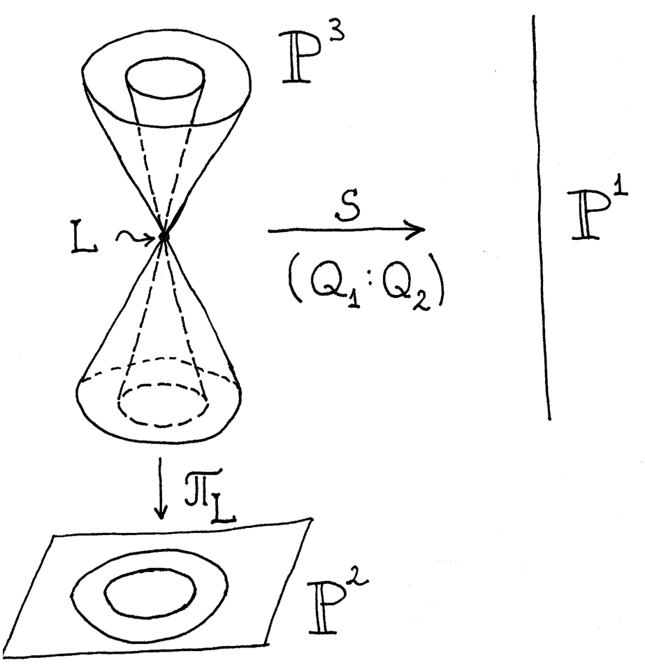
Example.
Consider the rational map
where are quadric cones with vertex . is dominant. Projection from the vertex to is also dominant, but the quadric cones (i.e. the fibers of ) do not map dominantly to (see Figure 1). The projection fibers are the lines through and indeed each such line is contained completely in one cone in the pencil .
The base locus of consists of lines that meet in . If on the other hand we project from a smooth point then a general fiber of maps dominantly to . Indeed a general line through intersects all cones.
The complications in proving ( arise due to the fact that the natural description of is in terms of the monomials which span it, whereas can be most easily evaluated on forms which are written as sums of powers of linear forms. These two points of view do not match, and we cannot repose on methods in [Shep]. Instead we introduce new techniques in section 5 to solve this difficulty:
- •
We use interpolation polynomials to write down elements in as sums of powers of linear forms.
- •
Next we employ considerations of leading terms (or, geometrically, jets at infinity) to eliminate the interpolation polynomials, from our formulae.
- •
For large enough , we finally reduce (4) to the property that a certain matrix has full rank. The size of is independent of while (and this is the main point) its entries are of the form
where are polynomials of fixed degree (i.e. independent of ), are constants, and the number of summands in the expression is independent of . This is possible only because we eliminated the interpolation polynomials in the previous step.
- •
By choosing a point with integer coefficients we can arrange that and are defined over with denominators that are not divisible by a small prime which we call the precision of our calculation. Thus if we work over the finite field , the matrix is periodic in with period . A computer algebra program is then used to check that these matrices all have full rank. By semicontinuity, this proves that has full rank for all in characteristic .
In a rather round-about sense, we have also been guided by the principle that evaluation of a polynomial at a special point can be much cheaper than computing the polynomial.
3. Notation and definition of the Covariants
For definiteness, the base field will be , the field of complex numbers, though one might replace it by any
algebraically closed field of characteristic throughout.
Let , and let be the
adjoint form of
. We denote by
the irreducible -representation . We fix a positive integer not divisible by , or , .
The symbol , , denotes the set of integers from (incl.) to (incl.). Let denote the basis dual to the standard basis in and put . We will use Schwartz’s multi-index notation and denote multi-indices by lower case boldface letters. Thus we write a
general homogeneous form of degree as
| (1) |
where , , , . We will use the symbolical method introduced by Aronhold and Clebsch to write down -equivariant maps (covariants) from to (if ) or to (if ). It is explained in [G-Y] and, from a modern point of view, in [Dol1], chapter 1. We denote by a vector of symbolic variables, and also introduce vectors , , , similarly. We write , and similarly , , . Moreover we define the bracket factor by
and write etc. similarly. The idea in this calculus is to write symbolically as a power of a linear form in several ways:
| (2) |
whence the identities
| (3) |
If , define a covariant of order and degree by the following prescription:
| (4) | ||||
| (5) |
The formula for should be read in the following way: The right hand side of , when we multiply it out formally, is a sum of monomials , , , and , . Thus one can use equations (1) and (3) to rewrite the right-hand-side unambiguously in terms of the coefficients of . Hence may be viewed as a map from to , homogeneous of degree in the coefficients , which is clearly -equivariant. By abuse of notation, we denote the induced rational map
| (6) |
by the same letter. Note that defined by equation may be viewed as an invariant of plane cubics of degree in the coefficients of the cubic. In fact, this is the famous Clebsch invariant, vanishing on the
locus of Fermat cubics, or vanishing on the equi-anharmonic cubics, i.e. nonsingular plane cubics which can be written as a
double cover of branched in four points with equi-anharmonic cross-ratio. Equi-anharmonic cross-ratio means
cross-ratio equal to minus a cube root of . Equi-anharmonic quadruples of points in are one of the two
possible
-orbits of points in with non-trivial isotropy group (the other orbit being
quadruples with harmonic cross-ratio, i.e. equal to , or ). See [D-K], (5.13), for details.
The letter in was chosen in honor of the 19th century Italian geometer Gaetano Scorza, who studied in detail the
map , called the Scorza map (cf. [D-K], §6 and §7, and [Dol2], section 6.4.1).
Similarly, for , we define a covariant of order and degree by
| (7) |
and denote the induced rational map by the same letter.
We remark that it is hard to calculate the values of (or ) on a general homogeneous form of degree without knowing the entire expression of (resp. ) as a polynomial in the coefficients , which is awkward. One can, however, work directly with the symbolic expressions given in (5) and (7) if one writes as a linear combination of -th powers of linear forms:
| (8) |
For linear forms , , , we use the notation
| (9) |
which is defined via formulas (4), (5), (7), but where for the vectors , , , of symbolic variables we substitute the vectors of coordinates w.r.t. , , of , , , and . One then has the following easy, but fundamental multi-linearity properties of and whose proof is a straight-forward computation and therefore omitted.
Lemma 3.1.
We have
| (10) | |||
| (11) |
The right-hand sums run over all with .
4. Special linear subspaces of the base loci
The group is a rank complex semisimple algebraic group, and choosing the standard torus of diagonal matrices as maximal torus, and the group of upper-triangular matrices as Borel subgroup, one has the notions of roots, positive and simple roots, and simple coroots , available. Corresponding to , one has one-parameter subgroups given by
For , we may view the covariant as an element in
| (18) |
a -invariant polynomial of degree in the curve coefficients , , , with values in . As such it is a linear combination of monomials
| (19) |
where , , , , , , .
Similarly, for , can be viewed as an element of
| (20) |
i.e. a -invariant polynomial of degree in the curve coefficients , , , with values in . It is a linear combination of monomials
| (21) |
where , , , , , , .
The following proposition is an important ingredient in the proof of rationality.
Proposition 4.1.
For , the projectivization of the linear space
| (22) |
is contained in the base scheme of the rational map
with a full triple structure, i.e.
Similarly, for , the projectivization of the linear space
| (23) |
is contained in the base scheme of
with a full triple structure.
Proof.
Regardless of whether or , the conditions that the monomials in (14) or (16) are invariant under the actions of the one-parameter subgroups resp. read
| (24) | ||||
| (25) |
Now for we get
| (26) | ||||
and for one has
| (27) | ||||
In both cases then it follows that
| (28) | ||||
In particular, for , , which means that at most out of the indices , , ,
can be . Since is generated by those with , this proves the
frist assertion.
For , , whence at most out of , , , can be , which proves the proposition.
∎
Remark 4.2.
By construction, (resp. ) have the following basic property: For (resp. ), the restriction (resp. ) is linear.
5. Fiberwise surjectivity of the covariants
To begin with, we will show how some elements of (resp. ) can be written as sums of powers. For this let be a positive integer.
Definition 5.1.
Let be given. Then we denote by
| (29) |
for the interpolation polynomials of degree w.r.t. in the one variable .
Lemma 5.2.
Let , for , and set , , . Suppose and put . Then for each with , ,
| (30) |
is nonzero and divisible by .
Proof.
The coefficient of the monomial in is equal to
For one has
for all by interpolation. ∎
Choosing , we obtain elements , and for elements . Now for consider the diagram
or for the diagram
The aim of this section is to prove
Proposition 5.3.
Let . Then there exists a such that
is surjective. For there exists a such that
is surjective.
We will prove the case first. The case is very similar, and we will deal with it afterwards.
We start by constructing points in the image :
Lemma 5.4.
Consider as an element of and write
| (31) |
with . Then for all .
Proof.
The map
| (32) | ||||
gives a rational normal curve in . Since by Remark 2.2, is linear, the linear span of is contained in . Now which proves the claim. ∎
Surprisingly, for large enough, the do not depend on the vector chosen to construct :
Proposition 5.5.
If
and
then for .
Proof.
Write as a sum of th powers of linear forms
| (33) |
where is a positive integer that will be fixed (independently of ) in the later discussion. Then (using and Lemma 3.1)
| (34) | ||||
For we find
| (35) | ||||
Since , the assertion follows. ∎
Next we will investigate the dependence of on for .
We choose a fixed constant (the “precision”) with and (later will be a prime number).
Lemma 5.6.
For , the coefficient of in is of the form
| (36) |
where (independent of and ) and is a polynomial of degree . is, as a polynomial in divisible by
If the coefficients of the are integers and is a prime number, then the reduction of the coefficient of in modulo is still of the form
| (37) |
whith and satifying the same independence and divisibility conditions as above.
Proof.
Calculating either over or over , we have
| (38) | |||
where the ’s and ’s are constants (fixed once the ’s are fixed). If any of the ’s vanishes the polynomials is of degree in . Since , in this situation the coefficient of is and we are finished. Assume therefore that the ’s are invertible.
The above expression expands to
and the coefficient of is
Put , , and rewrite this as
degree in ,and since , the coefficient of is then). The first claim of the lemma over is obvious now. The reductions of the binomial coefficients modulo are polynomials in over if . Our conditions on imply this, since
As for the stated divisibility property in and , remark that in
with , at least one of , , is . ∎
Proposition 5.7.
For , the coefficient of each monomial in is of the form
| (39) |
where are constants (independent of ), and are polynomials of degree ,
If can be written as sum of powers with integer coefficiens and is a prime number, the same is true for the reduction of mod .
Proof.
Definition 5.8.
For , we put
| (41) |
Proof of Proposition 5.3 (for ).
Let and consider
with
For we perform our construction with and two different values for , namely and . We obtain quartics . By Lemma 5.4 and Proposition 5.5 these quartics are in the image of if
The coefficients of the form a matrix with entries of the form by Proposition 5.7. Modulo this matrix becomes periodic in with period . With a computer algebra program it is straightforward to check that all these matrices have full rank . A Macaulay2 script doing this can be found at [BvB]. This proves the claim for . ∎
Let us turn to the case . The whole procedure is similar in this case. If we take Lemma 5.2, Proposition 5.5, Lemma 5.6 and Proposition 5.7 remain true as stated and Definition 5.8 still makes sense.
Proof of Proposition 5.3 (for ).
Let and consider
with as above.
For we perform our construction with and three different values for , namely , and . We obtain octics . By Lemma 5.4 and Proposition 5.5 these octics are in the image of if
The coefficients of the from a matrix with entries of the form by Proposition 5.7. Modulo this matrix becomes periodic in with period . With a computer algebra program it is straightforward to check that all these matrices have full rank . A Macaulay2 script doing this can be found at [BvB]. This proves the claim for . ∎
6. Sections of principal bundles and proof of rationality
We will now show how to conclude the proof in the case . We make some comments on the case when they are in order, but otherwise leave the obvious modifications to the reader. Let be the open subset of very stable points with respect to the action of and the -linearized line bundle (very stable means stable with trivial stabilizer). Now the essential point is
Proposition 6.1.
The quotient morphism
is a principal -bundle in the Zariski topology.
Proof.
See [Shep], Prop. 2. This holds also true with replaced with . ∎
It follows that this -bundle has a section defined generically which we will denote by .
Proof of Theorem 1.1.
Consider the incidence variety
and the diagram
By Proposition 5.3 the projection is dominant. It follows then from Remark 4.2 that is birational to a vector bundle over and hence also over . After replacing by a translate, we can assume that meets an open set over which is trivial. Since acts generically freely on , we can pull back the above vector bundle structure via and obtain that is birational to with . If as in Proposition 5.3, then certainly and since is rational, is rational. In the case the same argument works since the space of octics is also stably rational of level . This proves Theorem 1.1. ∎
References
- [A-M] Artin, M. & Mumford, D., Some elementary examples of unirational varieties which are not rational, Proc. London Math. Soc. (3) 25 (1972), 75-95
- [Beau] Beauville, A., Colliot-Thélène, J.-L., Sansuc, J.-J., Swinnerton-Dyer, Sir Peter, Variétés stablement rationalles non-rationelles, Annals of Math. 121 (1985), 283-318
- [Be] Beklemishev, N., Invariants of cubic forms in four variables, Vestnik Moscov. Univ. Ser. I Mat. Mekh. 2 (1982), 42-49
- [Bog1] Bogomolov, F., Stable rationality of quotient varieties by simply connected groups, Mat. Sbornik 130 (1986), 3-17
- [Bog2] Bogomolov, F., Rationality of the moduli of hyperelliptic curves of arbitrary genus, (Conf. Alg. Geom., Vancouver 1984), CMS Conf. Proceedings vol. 6, Amer. Math. Soc., Providence, R.I. (1986), 17-37
- [Bo-Ka] Bogomolov, F. & Katsylo, P., Rationality of some quotient varieties, Mat. Sbornik 126 (1985), 584-589
- [BvB] Christian Böhning and H.-Chr. Graf v. Bothmer. Macalaulay2 scripts to check the surjectivity of the Scorza and Octa maps. Available at http://www.uni-math.gwdg.de/bothmer/rationality, 2008.
- [C-G] Clemens, H. & Griffiths, P., The intermediate Jacobian of the cubic threefold, Ann. of Math. 95 (1972), 281-356
- [D-K] Dolgachev, I. & Kanev, V., Polar Covariants of Plane Cubics and Quartics, Advances in Mathematics 98 (1993), 216-301
- [Dol0] Dolgachev, I., Rationality of Fields of Invariants, Proceedings of Symposia in Pure Mathematics vol. 46 (1987), 3-16
- [Dol1] Dolgachev, I., Lectures on Invariant Theory, London Mathematical Society Lecture Note Series 296, Cambridge Univ. Press (2003)
- [Dol2] Dolgachev, I., Topics in Classical Algebraic Geometry. Part I, available at http://www.math.lsa.umich.edu/ idolga/lecturenotes.html
- [G-Y] Grace, J.H. & Young, W.H., The Algebra of Invariants, Cambridge Univ. Press (1903); reprinted by Chelsea Publ. Co. New York (1965)
- [I-K] Iarrobino, A. & Kanev, V., Power Sums, Gorenstein Algebras, and Determinantal Loci, Springer Lecture Notes in Mathematics 1721, Springer-Verlag (1999)
- [Is-Pr] Iskovskikh, V.A. & Prokhorov, Yu.G., Fano Varieties, Encyclopedia of Math. Sciences Vol. 47, Algebraic Geometry V, A.N. Parshin, I.R. Shafarevich (Eds.), Springer-Verlag Berlin Heidelberg (1999)
- [Kat] Katsylo, P.I., Rationality of the moduli spaces of hyperelliptic curves, Izv. Akad. Nauk SSSR Ser. Mat. 48 (1984), 705-710
- [Kat0] Katsylo, P.I., Rationality of moduli varieties of plane curves of degree , Math. USSR Sbornik, Vol. 64, no. 2 (1989)
- [Kat1] Katsylo, P.I., On the birational geometry of the space of ternary quartics, Advances in Soviet Math. 8 (1992), 95-103
- [Kat2] Katsylo, P.I., Rationality of the moduli variety of curves of genus , Comment. Math. Helvetici 71 (1996), 507-524
- [Muk] Mukai, S., Fano 3-folds, in: Complex Projective Geometry, London Mathematical Society L. N. S. 179, Cambridge University Press (1992), 255-263
- [Mum] Mumford, D., Fogarty, J., Kirwan, F., Geometric Invariant Theory, Third Enlarged Edition, Ergebnisse der Mathematik und ihrer Grenzgebiete 34, Springer-Verlag (1994)
- [R-S] Ranestad, K. & Schreyer, F., Varieties of sums of powers, J. Reine Angew. Math. 525 (2000), 147-181
- [Sa] Saltman, D., Noether’s problem over an algebraically closed field, Invent. Math. 77 (1984), 71-84
- [Shep] Shepherd-Barron, N.I., The rationality of some moduli spaces of plane curves, Compositio Mathematica 67 (1988), 51-88