跳到论文正文
W Papers独立论文阅读器 arXiv:0804.1360 论文正文 计算阅读时间 · 0%
引用这篇论文根据当前论文元数据生成,正式投稿前建议核对。


License: arXiv.org perpetual non-exclusive license
arXiv:0804.1360v1 [gr-qc] 08 Apr 2008

Brownian Motion in Robertson-Walker Space-Times from Electromagnetic Vacuum Fluctuations

Carlos H. G. Béssa Email: carlos@cosmos.phy.tufts.edu Affiliation: Institute of Cosmology, Department of Physics and Astronomy,
Tufts University, Medford, MA 02155 USA
Affiliation: Departamento de Física, Universidade Federal da Paraíba,
João Pessoa, PB 58051-970, Brazil
   Valdir B. Bezerra Email: valdir@fisica.ufpb.br Affiliation: Departamento de Física, Universidade Federal da Paraíba,
João Pessoa, PB 58051-970, Brazil
   L. H. Ford Email: ford@cosmos.phy.tufts.edu Affiliation: Institute of Cosmology, Department of Physics and Astronomy,
Tufts University, Medford, MA 02155 USA
Abstract

We consider classical particles coupled to the quantized electromagnetic field in the background of a spatially flat Robertson-Walker universe. We find that these particles typically undergo Brownian motion and acquire a non-zero mean squared velocity which depends upon the scale factor of the universe. This Brownian motion can be interpreted as due to non-cancellation of anti-correlated vacuum fluctuations in the time dependent background space-time. We consider several types of coupling to the electromagnetic field, including particles with net electric charge, a magnetic dipole moment, and electric polarizability. We also investigate several different model scale factors.

pacs
04.62.+v,05.40.Jc,12.20.-m

I Introduction

Brownian motion of a particle in a thermal bath is a well-known phenomenon. (See, for example, Ref. [1].) In this case, the particle’s mean squared velocity grows linearly in time until dissipation effects become important, after which it approaches a non-zero equilibrium value. The linear growth phase is characteristic of any random walk process, in which each fluctuation is independent of previous fluctuations. Quantum fluctuations are quite different from thermal ones in that the former are strongly correlated or anti-correlated. This does not, however, prevent quantum Brownian motion, which will be the topic of this paper. The existence of Brownian motion in the Minkowski vacuum state is controversial. Although conventional quantum electrodynamics suggests that the only effect will be an unobservable mass renormalization, Gour and Sriramkumar [2] have argued that there could be an observable effect on charged particles coupled to the fluctuating electromagnetic field. Brownian motion in the presence of boundaries is less controversial, and has been studied by several authors [3, 4, 5, 6, 7, 8]. Barton [3] was the first to examine fluctuations of the Casimir force. Wu et al [5] calculated the Brownian motion of an atom near a perfectly reflecting plate due to fluctuations in the retarded van der Waals force. The mean force here is the Casimir-Polder force [9]. The analogous Brownian motion of a charged particle near a reflecting plate was treated by Yu and Ford [6]. In all of these cases, the mean squared velocity of the particle approaches a constant even in the absence of dissipation. This is required by energy conservation, as there is no energy source in these static configurations. The fact that the late time mean squared velocity is non-zero can be attributed to the effects of switching when the interaction is turned on. Switching effects were recently discussed by Seriu and Wu [8].

The mechanism which enforces the lack of growth of the mean squared velocity can be understood as anti-correlated fluctuations. A charged or polarizable particle in a Casimir vacuum can acquire an energy EE from a fluctuation. However, that energy is typically surrendered on a time scale of order ℏ/E\hbar/E to an anti-correlated fluctuation. The correlation functions of the quantized electromagnetic field automatically enforces the required anti-correlations [10]. The quantum fluctuations of the stress tensor in flat spacetime also exhibits subtle correlations and anti-correlations, as is discussed in Ref. [11].

The Brownian motion of test particles is an operational means to describe a fluctuating quantum field. This approach can be used to treat the quantum fluctuations of the gravitational field, which has been a topic of much interest in recent years [12, 13, 14, 15, 16, 17, 18, 19, 20, 21, 22, 23, 24, 25].

In the present paper, we will investigate the Brownian motion of various types of particles coupled to the quantized electromagnetic field in the background of a Robertson-Walker spacetime. Here the time-dependent background geometry can act as an energy source, so the particles can acquire a net kinetic energy.

In Sect. II we develop the basic Langevin equation formalism for calculating the mean squared velocity of classical particles coupled to a fluctuating force in a spatially flat Robertson-Walker background. The formalism is applied to a several specific choices for the scale factor of the universe in Sect. III. Our results are summarized and discussed in Sect. IV.

Unless otherwise noted, we work in Lorentz-Heaviside units with ℏ=c=1\hbar=c=1.

II Basic Formalism

The equation of motion of a classical point particle moving in a curved spacetime with a four-force fμf^{\mu} is

fμ=m​D​uμd​τ,f^{\mu}=m\frac{Du^{\mu}}{d\tau}\,, (1)

where uμu^{\mu} is the 4-velocity of the particle, mm is its mass and τ\tau the proper time. The operator D/d​τD/d\tau on the right-hand side of Eq. (1) is the covariant derivative given by

D​uμd​τ=d​uμd​τ+Γα​βμ​uα​uβ.\frac{Du^{\mu}}{d\tau}=\frac{du^{\mu}}{d\tau}+\Gamma^{\mu}_{\alpha\beta}u^{\alpha}u^{\beta}\,. (2)

Here we take the space-time geometry to be that of a spatially flat Robertson-Walker universe with metric

d​s2=−d​t2+a2​(t)​(d​x2+d​y2+d​z2),ds^{2}=-dt^{2}+a^{2}(t)(dx^{2}+dy^{2}+dz^{2})\,, (3)

where a⁡(t)a(t) is the scale factor. We will restrict our attention to the case where the particles are moving slowly with respect to these coordinates, in which case the particle’s proper time becomes the coordinate time tt. Because of spatial isotropy, we can consider a particular direction, the xx-direction, and write the equation of motion as

d​uxd​t+2​a˙a​ux=1m​fx.\frac{du^{x}}{dt}+2\frac{\dot{a}}{a}u^{x}=\frac{1}{m}f^{x}\,. (4)

Here we have used Γt​xx=Γx​tx=a˙/a\Gamma^{x}_{tx}=\Gamma^{x}_{xt}=\dot{a}/a, where a˙=d​a/d​t\dot{a}=da/dt. We will take the four-force to be of the form

fx=fx′+fe​x​tx,f^{x}=f^{{}^{\prime}x}+f^{x}_{ext}\,, (5)

where fe​x​txf^{x}_{ext} is a non-fluctuating external force, and f′xf^{\prime x} is a fluctuating force produced by the electromagnetic vacuum fluctuations whose mean value vanishes:

⟨fx′⟩=0.\langle f^{{}^{\prime}x}\rangle=0\,. (6)

First, let us consider the case of free particles, which corresponds to the case when fe​x​t=0f_{ext}=0. Thus Eq. (4) can be written as,

1a2​dd​t​(a2​ux)=fx′m,\frac{1}{a^{2}}\frac{d}{dt}\left(a^{2}u^{x}\right)=\frac{f^{{}^{\prime}x}}{m}, (7)

which after integration reduces to

a2​(tf)​ux​(tf)−a2​(t0)​ux​(t0)=1m​∫t0tfd​t​a2​(t)​fx′​(t).a^{2}(t_{f})u^{x}(t_{f})-a^{2}(t_{0})u^{x}(t_{0})=\frac{1}{m}\int_{t_{0}}^{t_{f}}dta^{2}(t)f^{{}^{\prime}x}(t). (8)

Assuming that these particles are initially at rest (ux​(t0)=0u^{x}(t_{0})=0), we find that the velocity-velocity correlation function is given by

⟨ux​(tf,r1)​ux​(tf,r2)⟩=1m2​af4​∫d​t1​d​t2​a2​(t1)​a2​(t2)​⟨fx′​(t1,r1)​fx′​(t2,r2)⟩.\langle u^{x}(t_{f},r_{1})u^{x}(t_{f},r_{2})\rangle=\frac{1}{m^{2}a_{f}^{4}}\int dt_{1}dt_{2}a^{2}(t_{1})a^{2}(t_{2})\;\langle f^{{}^{\prime}x}(t_{1},r_{1})f^{{}^{\prime}x}(t_{2},r_{2})\rangle\,. (9)

Another case of interest is when there is an external force which cancels the effect of the cosmological expansion:

fe​x​tx=2​a˙a​ux.f^{x}_{ext}=2\frac{\dot{a}}{a}\,u^{x}\,. (10)

This is the case for any particles in bound systems such as galaxies or molecules. Such particles do not participate in the cosmological expansion and in this case two such particles do not move apart on the average. We will refer to these as bound particles. In this case,

d​uxd​t=1m​f′x,\frac{du^{x}}{dt}=\frac{1}{m}f^{\prime x}\,, (11)

and the velocity correlation functions for particles which start at rest at t=tft=t_{f} is

⟨ux​(tf,r1)​ux​(tf,r2)⟩=1m2​∫d​t1​d​t2​⟨fx′​(t1,r1)​fx′​(t2,r2)⟩.\langle u^{x}(t_{f},r_{1})u^{x}(t_{f},r_{2})\rangle=\frac{1}{m^{2}}\int dt_{1}dt_{2}\,\langle f^{{}^{\prime}x}(t_{1},r_{1})f^{{}^{\prime}x}(t_{2},r_{2})\rangle\,. (12)

Note that the above expression is a coordinate velocity correlation function. In a Robertson-Walker space-time, proper distance between particles, lfl_{f}, is related to the coordinate separation rr at t=tft=t_{f} by lf=af​rl_{f}=a_{f}r. Thus the proper velocity correlation function is given by

⟨vx​(tf,r1)​vx​(tf,r2)⟩=af2​⟨ux​(tf,r1)​ux​(tf,r2)⟩.\langle v^{x}(t_{f},r_{1})v^{x}(t_{f},r_{2})\rangle=a_{f}^{2}\langle u^{x}(t_{f},r_{1})u^{x}(t_{f},r_{2})\rangle\,. (13)

II.1 Charged Particles

In this section, we will consider electrically charged particles with charge qq coupled to a fluctuating electromagnetic field. In this case, the four-force is

f′x=qm​Fx​t​ut≈−qm​Fx​t.f^{\prime x}=\frac{q}{m}F^{xt}u_{t}\approx-\frac{q}{m}F^{xt}\,. (14)

For the case of free particles, Eq. (9) yields

⟨ux​(tf,r1)​ux​(tf,r2)⟩=q24​af4​∫d​t1​∫d​t2​a2​(t1)​a2​(t2)​⟨(Fx​t​ut)1​(Fx​t​ut)2⟩R​W,\langle u^{x}(t_{f},r_{1})u^{x}(t_{f},r_{2})\rangle=\frac{q^{2}}{4a_{f}^{4}}\int dt_{1}\int dt_{2}\;a^{2}(t_{1})a^{2}(t_{2})\,\langle\left(F^{xt}u_{t}\right)_{1}\left(F^{xt}u_{t}\right)_{2}\rangle_{RW}, (15)

where the sub-indexes 1 and 2 refer to the coordinates (t1,r1)(t_{1},r_{1}) and (t2,r2)(t_{2},r_{2}), respectively, and the subscript R​WRW denotes a vacuum correlation function in Robertson-Walker spacetime.

This correlation function is obtained from the corresponding correlation function in flat spacetime by a conformal transformation. First write the Robertson-Walker metric in its conformal form

d​s2=a2​(−d​η2+d​x2+d​y2+d​z2),ds^{2}=a^{2}(-d\eta^{2}+dx^{2}+dy^{2}+dz^{2}), (16)

with d​t=a​d​ηdt=ad\eta. The field strength tensor in these coordinates is given by

(Fμ​ν)R​W=a−4​(Fμ​ν)M,\left(F^{\mu\nu}\right)_{RW}=a^{-4}\left(F^{\mu\nu}\right)_{M}\,, (17)

where the subscript MM refers to the Minkowski space field strength. This may be seen, for example, from the fact that the Lagrangian density, −g​Fμ​ν​Fμ​ν\sqrt{-g}F^{\mu\nu}F_{\mu\nu} is invariant under the conformal transformation. From this and Eq. (15), we find

⟨ux​(tf,r1)​ux​(tf,r2)⟩=q2m2​af4​∫d​η1​∫d​η2​⟨Fη​x​(η1,r1)​Fη​x​(η2,r2)⟩M.\langle u^{x}(t_{f},r_{1})u^{x}(t_{f},r_{2})\rangle=\frac{q^{2}}{m^{2}a_{f}^{4}}\int d\eta_{1}\int d\eta_{2}\,\langle F^{\eta x}(\eta_{1},r_{1})F^{\eta x}(\eta_{2},r_{2})\rangle_{M}\,. (18)

Here the appropriate component of the Minkowski space correlation function is given by Eq. (126). The key feature of this result is that the scale factor does not appear inside the integrand. Thus the cosmological expansion has no effect on the Brownian motion, and hence we do not find an interesting result in this case.

The case of bound charged particles is different. In this case, from Eqs. (12) and (126), we find

⟨ux​(η,r1)​ux​(η,r2)⟩=q2m2​∫d​η1​∫d​η2​⟨(Ft​x​ut)1​(Ft​x​ut)2⟩R​W\displaystyle\langle u^{x}(\eta,r_{1})u^{x}(\eta,r_{2})\rangle=\frac{q^{2}}{m^{2}}\int d\eta_{1}\int d\eta_{2}\langle\left(F^{tx}u_{t}\right)_{1}\left(F^{tx}u_{t}\right)_{2}\rangle_{RW} (19)
=q2m2​∫d​η1​∫d​η2​a−2​(η1)​a−2​(η2)​{−(η2−η1)2−r′2π2​[−(η2−η1)2+r2]3}.\displaystyle=\frac{q^{2}}{m^{2}}\int d\eta_{1}\int d\eta_{2}\;a^{-2}(\eta_{1})a^{-2}(\eta_{2})\,\left\{\frac{-(\eta_{2}-\eta_{1})^{2}-r^{\prime 2}}{\pi^{2}[-(\eta_{2}-\eta_{1})^{2}+r^{2}]^{3}}\right\}\,.

Here rr is the spatial separation of the particles and r′2=r2−2​Δ​x2r^{\prime 2}=r^{2}-2\Delta x^{2}. Now there are factors of 1/a21/a^{2} in the integrand, which will lead to non-trivial effects in an expanding universe.

II.2 Magnetic Dipoles

In this section we will consider particles with a magnetic dipole moment. In flat spacetime, such particles experience a force when there is a non-zero magnetic field gradient:

f→=−∇u\vec{f}=-\nabla u (20)

where u=−μ→.B→u=-\vec{\mu}.\vec{B}, is the magnetic potential energy, μ\mu is the magnetic moment and B→\vec{B} is the magnetic field. Writing this force in covariant form, we have for the xx-component

fx=μ​∂x(Fz​y​xz​xy′)f^{x}=\mu\partial^{x}\left(F^{zy}x_{z}x^{\prime}_{y}\right) (21)

where, xμ=(0,0,0,a)x_{\mu}=(0,0,0,a) and xμ′=(0,0,a,0)x^{\prime}_{\mu}=(0,0,a,0), and such that xμ​xμ=x′μ​xμ′=1x^{\mu}x_{\mu}=x^{\prime\mu}x^{\prime}_{\mu}=1.

For free particles, the velocity-velocity correlation function, Eq. (9), becomes

⟨ux​(tf,r1)​ux​(tf,r2)⟩=μ2a4​(tf)​m2​∫d​t1​∫d​t2​∂x1∂x2⟨(Fz​y​xz​xy′)1​(Fz​y​xz​xy′)2⟩R​W.\langle u^{x}(t_{f},r_{1})u^{x}(t_{f},r_{2})\rangle=\frac{\mu^{2}}{a^{4}(t_{f})m^{2}}\int dt_{1}\int dt_{2}\partial_{x_{1}}\partial_{x_{2}}\,\langle\left(F^{zy}x_{z}x^{\prime}_{y}\right)_{1}\left(F^{zy}x_{z}x^{\prime}_{y}\right)_{2}\rangle_{RW}. (22)

Again, we may use Eq. (17) to write the above expression in terms of ∂x1∂x2⟨Fz​y​(η1,r1)​Fz​y​(η2,r2)⟩M\partial_{x_{1}}\partial_{x_{2}}\langle F^{zy}(\eta_{1},r_{1})\,F^{zy}(\eta_{2},r_{2})\rangle_{M}, which may be evaluated to write

⟨ux(η,r1)ux(η,r2)⟩=−μ2m2​a4​(tf)∫dη1∫dη2a−1(η1)a−1(η2)×\displaystyle\langle u^{x}(\eta,r_{1})u^{x}(\eta,r_{2})\rangle=-\frac{\mu^{2}}{m^{2}a^{4}(t_{f})}\int d\eta_{1}\int d\eta_{2}a^{-1}(\eta_{1})a^{-1}(\eta_{2})\times (23)
{2[−(η2−η1)2+r2]3+6​(η2−η1)2[−(η2−η1)2+r2]4}.\displaystyle\left\{\frac{2}{\left[-(\eta_{2}-\eta_{1})^{2}+r^{2}\right]^{3}}+\frac{6(\eta_{2}-\eta_{1})^{2}}{\left[-(\eta_{2}-\eta_{1})^{2}+r^{2}\right]^{4}}\right\}.

In Eq. (23), we have used the coincident limit r→0r\rightarrow 0 only in the numerator, in order to simplify our expressions. This will not alter our final results, because we will take this limit after the integrations.

For bound magnetic dipoles, we may start with Eq. (12) and follow the same procedure to find

⟨ux​(η,r1)​ux​(η,r2)⟩\displaystyle\langle u^{x}(\eta,r_{1})u^{x}(\eta,r_{2})\rangle =−μ2m2∫dη1∫dη2a−3(η1)a−3(η2)×\displaystyle=-\frac{\mu^{2}}{m^{2}}\int d\eta_{1}\int d\eta_{2}a^{-3}(\eta_{1})a^{-3}(\eta_{2})\times (24)
{2[−(η2−η1)2+r2]3+6​(η2−η1)2[−(η2−η1)2+r2]4},\displaystyle\left\{\frac{2}{\left[-(\eta_{2}-\eta_{1})^{2}+r^{2}\right]^{3}}+\frac{6(\eta_{2}-\eta_{1})^{2}}{\left[-(\eta_{2}-\eta_{1})^{2}+r^{2}\right]^{4}}\right\},

where again the coincidence limit in the spatial coordinate was taken in the numerator of the integrand.

II.3 Polarizable Particle

We will consider in this section a polarizable particle, described as a point particle with a static polarizability α\alpha. In an inhomogeneous electric field, such a particle experiences a force

f→(x)=α2∇(E2),\vec{f}(x)=\frac{\alpha}{2}\nabla(E^{2})\,, (25)

which in covariant notation becomes,

fx=α2​∂x(Ft​x​ut​xx)2,f^{x}=\frac{\alpha}{2}\partial^{x}\left(F^{tx}u_{t}x_{x}\right)^{2}, (26)

where the low velocity limit was taken with uν=−δν0u_{\nu}=-\delta^{0}_{\nu}, xμ=(0,a,0,0)x_{\mu}=(0,a,0,0). For a free particle, Eqs. (9) and (26) lead to

⟨ux​(tf,r1)​ux​(tf,r2)⟩\displaystyle\langle u^{x}(t_{f},r_{1})u^{x}(t_{f},r_{2})\rangle =α24​af4∫dη1∫dη2×\displaystyle=\frac{\alpha^{2}}{4a_{f}^{4}}\int d\eta_{1}\int d\eta_{2}\times (27)
a−3​(η1)​a−3​(η2)​∂x1∂x2⟨[F0​i​(η1,r1)]2​[F0​i​(η2,r2)]2⟩M,\displaystyle a^{-3}(\eta_{1})a^{-3}(\eta_{2})\partial_{x_{1}}\partial_{x_{2}}\langle\left[F^{0i}(\eta_{1},r_{1})\right]^{2}\left[F^{0i}(\eta_{2},r_{2})\right]^{2}\rangle_{M},

where we used the fact that uμ=−a​δμηu_{\mu}=-a\delta_{\mu}^{\eta} and xμ=(0,a,0,0)x_{\mu}=(0,a,0,0), in conformal coordinates.

Here we use the Wick theorem to calculate the two-point function: ⟨E2​(r1)​E2​(r2)⟩M=⟨Ei​(r1)​Ei​(r2)​Ej​(r1)​Ej​(r2)⟩M\langle E^{2}(r_{1})E^{2}(r_{2})\rangle_{M}=\langle E_{i}(r_{1})E^{i}(r_{2})E_{j}(r_{1})E^{j}(r_{2})\rangle_{M}, finding

⟨Ei​(r1)​Ei​(r2)​Ej​(r1)​Ej​(r2)⟩M=2​[⟨Ei​(r1)​Ej​(r2)⟩M​⟨Ei​(r1)​Ej​(r2)⟩M],\langle E_{i}(r_{1})E^{i}(r_{2})E_{j}(r_{1})E^{j}(r_{2})\rangle_{M}=2\left[\langle E_{i}(r_{1})E_{j}(r_{2})\rangle_{M}\langle E^{i}(r_{1})E^{j}(r_{2})\rangle_{M}\right], (28)

or, from the procedure outlined in Appendix A,

⟨Ei​(r1)​Ei​(r2)​Ej​(r1)​Ej​(r2)⟩M={−3​(η2−η1)2−r2π2​[−(η2−η1)2+r2]3}2.\langle E_{i}(r_{1})E^{i}(r_{2})E_{j}(r_{1})E^{j}(r_{2})\rangle_{M}=\left\{\frac{-3(\eta_{2}-\eta_{1})^{2}-r^{2}}{\pi^{2}[-(\eta_{2}-\eta_{1})^{2}+r^{2}]^{3}}\right\}^{2}\,. (29)

To simplify our expression we will consider the coincident limit in the spatial coordinate r=r2−r1=0r=r_{2}-r_{1}=0, only in the numerator of all factors, as in the previous cases. Then the velocity-velocity correlation function is,

⟨ux(η,r1)ux(η,r2)⟩=α24​m2​af4∫dη1∫dη2a−3(η1)a−3(η2)×\displaystyle\langle u^{x}(\eta,r_{1})u^{x}(\eta,r_{2})\rangle=\frac{\alpha^{2}}{4m^{2}a_{f}^{4}}\int d\eta_{1}\int d\eta_{2}a^{-3}(\eta_{1})a^{-3}(\eta_{2})\times (30)
{32[−(η2−η1)2+r2]5+136​(η2−η1)2[−(η2−η1)2+r2]6+144​(η2−η1)4[−(η2−η1)2+r2]7}.\displaystyle\left\{\frac{32}{[-(\eta_{2}-\eta_{1})^{2}+r^{2}]^{5}}+\frac{136(\eta_{2}-\eta_{1})^{2}}{[-(\eta_{2}-\eta_{1})^{2}+r^{2}]^{6}}+\frac{144(\eta_{2}-\eta_{1})^{4}}{[-(\eta_{2}-\eta_{1})^{2}+r^{2}]^{7}}\right\}.

III Specific Universe Models

In this section we will apply the basic formulas obtained in Sect. II to investigate the influence of different scale factors on the Brownian motion of particles induced by quantum vacuum fluctuations of the electromagnetic field.

III.1 Asymptotically Static Bouncing Universe

The study of bouncing universe was considered by some authors in the past [26]. Here we will study a special case, which is asymptotically static in the past and future. We will take the scale factor to have the form

an=η2+η02η2+G2​η02,a^{n}=\frac{\eta^{2}+\eta_{0}^{2}}{\eta^{2}+G^{2}\eta_{0}^{2}}, (31)

where GG and η0\eta_{0} are constants, and nn is a positive integer. Note that when η→±∞\eta\rightarrow\pm\infty, the universe is asymptotically flat and aa goes to unity. It will be convenient to consider different choices of nn for different types of particles in order to simplify the corresponding integrals.

III.1.1 Bound Charged Particles

In this case, we set n=1n=1, so that Eq. (19) becomes

⟨Δ​u​(η,r1)​Δ​u​(η,r2)⟩=q2m2​∫−∞+∞d​η1​∫−∞+∞d​η2​(η12+G2​η02η12+η02)2\displaystyle\langle\Delta u(\eta,r_{1})\Delta u(\eta,r_{2})\rangle=\frac{q^{2}}{m^{2}}\int_{-\infty}^{+\infty}d\eta_{1}\int_{-\infty}^{+\infty}d\eta_{2}\left(\frac{\eta_{1}^{2}+G^{2}\eta_{0}^{2}}{\eta_{1}^{2}+\eta_{0}^{2}}\right)^{2} (32)
×(η22+G2​η02η22+η02)2​[−(η2−η1)2−r2′π2​[−(η2−η1)2+r2]3],\displaystyle\times\left(\frac{\eta_{2}^{2}+G^{2}\eta_{0}^{2}}{\eta_{2}^{2}+\eta_{0}^{2}}\right)^{2}\left[\frac{-(\eta_{2}-\eta_{1})^{2}-r^{{}^{\prime}2}}{\pi^{2}[-(\eta_{2}-\eta_{1})^{2}+r^{2}]^{3}}\right],

where we used Eq. (19). This integral is evaluated in Appendix B, with the result being a rather complicated expression, Eq. (129). This result simplifies considerably in the limit that r1→r2r_{1}\rightarrow r_{2} and G≫1G\gg 1 to

⟨Δ​u2⟩=21​q2​G8128​m2​η02.\langle\Delta u^{2}\rangle=\frac{21q^{2}G^{8}}{128m^{2}\eta_{0}^{2}}. (33)

Note that because af=1a_{f}=1, this expression also gives the mean squared proper velocity ⟨Δ​v2⟩\langle\Delta v^{2}\rangle.

We can gain some insight into this result by writing it in terms of a characteristic measure of the maximum curvature. Consider the scalar curvature RR and evaluate it using the scale factor Eq. (31) with n=1n=1. We find the following result,

R0=12​G2η02​(1−G2),R_{0}=\frac{12G^{2}}{\eta_{0}^{2}}\left(1-G^{2}\right), (34)

where R0R_{0} is the Ricci scalar when η=0\eta=0. If we consider the limit G≫1G\gg 1, R0R_{0} is negative and

R02≈144​G8η04.R_{0}^{2}\approx\frac{144G^{8}}{\eta_{0}^{4}}. (35)

Then ⟨Δ​v2⟩\langle\Delta v^{2}\rangle in terms of R0R_{0} is

⟨Δ​v2⟩=7​q2​η02​R026144​m2.\langle\Delta v^{2}\rangle=\frac{7q^{2}\eta_{0}^{2}R_{0}^{2}}{6144m^{2}}. (36)

We can also write Eq. (36) in terms of the redshift, defined by: am−2≡(1+z)2a_{m}^{-2}\equiv(1+z)^{2}, with am≡a⁡(0)/a⁡(∞)=(1/G)2a_{m}\equiv a(0)/a(\infty)=(1/G)^{2}, where ama_{m} is the minimum scale factor. Considering z≫1z\gg 1, we get

⟨Δ​v2⟩=7​q2​|R0|6144​m2​z2.\langle\Delta v^{2}\rangle=\frac{7q^{2}|R_{0}|}{6144m^{2}}z^{2}. (37)

The mean squared velocity is proportional both to the squared redshift and to the maximum curvature. This can be associated with an effective temperature using the non-relativistic equation: kB​Te​f​f=m⁡⟨Δ​v2⟩k_{B}T_{eff}=m\langle\Delta v^{2}\rangle. Where Te​f​fT_{eff} is the effective temperature and kBk_{B} is the Boltzmann constant in Lorentz-Heaviside units ℏ=c=1\hbar=c=1. Then, Te​f​fT_{eff} is,

Te​f​f≃10−3​q2kB​λc​(λclc)2​z2,T_{eff}\simeq\frac{10^{-3}q^{2}}{k_{B}\lambda_{c}}\left(\frac{\lambda_{c}}{l_{c}}\right)^{2}z^{2}, (38)

where lc=1/|R0|l_{c}=1/\sqrt{|R_{0}|} is the lenght curvature and λc=1/m\lambda_{c}=1/m is the particle’s Compton wavelength.

III.1.2 Free Magnetic Dipoles

Again take the scale factor to be Eq. (31) with n=1n=1. Then Eq. (23) for the mean squared velocity becomes,

⟨Δ​u​(r1,η)​Δ​u​(r2,η)⟩\displaystyle\langle\Delta u(r_{1},\eta)\Delta u(r_{2},\eta)\rangle =\displaystyle= μ2af4​m2​∫−∞∞d​η1​∫−∞∞d​η2​(η2+G2​η02η12+η02)​(η2+G2​η02η22+η02)\displaystyle\frac{\mu^{2}}{a_{f}^{4}m^{2}}\;\int^{\infty}_{-\infty}d\eta_{1}\int^{\infty}_{-\infty}d\eta_{2}\left(\frac{\eta^{2}+G^{2}\eta_{0}^{2}}{\eta_{1}^{2}+\eta_{0}^{2}}\right)\left(\frac{\eta^{2}+G^{2}\eta_{0}^{2}}{\eta_{2}^{2}+\eta_{0}^{2}}\right) (39)
×\displaystyle\times {−2[−(η2−η1)2+r2]3−6​(η2−η1)2[−(η2−η1)2+r2}.\displaystyle\left\{\frac{-2}{[-(\eta_{2}-\eta_{1})^{2}+r^{2}]^{3}}-\frac{6(\eta_{2}-\eta_{1})^{2}}{[-(\eta_{2}-\eta_{1})^{2}+r^{2}}\right\}.

Using the same procedure as before, we find the following result in the coincident limit when G≫1G\gg 1

⟨Δ​v2⟩=10−3​μ2m2​|R0|η02.\langle\Delta v^{2}\rangle=\frac{10^{-3}\mu^{2}}{m^{2}}\frac{|R_{0}|}{\eta_{0}^{2}}. (40)

In terms of the redshift (z≫1z\gg 1), we have

⟨Δ​v2⟩=10−3​μ2m2​|R0|2z2.\langle\Delta v^{2}\rangle=\frac{10^{-3}\mu^{2}}{m^{2}}\frac{|R_{0}|^{2}}{z^{2}}. (41)

In contrast to the result for bound charges, the effect decreases with zz. For the case of electrons, it is convenient to write the magnetic moment as

μ≃q2​m.\mu\simeq\frac{q}{2m}\,. (42)

The effective temperature in terms of curvature length and Compton wavelength λc\lambda_{c} is,

Te​f​f=10−3​q2λc​kB​(λclc)4​z−2.T_{eff}=\frac{10^{-3}q^{2}}{\lambda_{c}k_{B}}\left(\frac{\lambda_{c}}{l_{c}}\right)^{4}z^{-2}. (43)

III.1.3 Bound Magnetic Dipoles

Here we choose the scale factor to be of the form of Eq. (31) with n=3n=3. In this case, the mean squared velocity from Eq. (24) is,

⟨Δ​u​(r1,η)​Δ​u​(r2,η)⟩\displaystyle\langle\Delta u(r_{1},\eta)\Delta u(r_{2},\eta)\rangle =\displaystyle= μ2m2​∫−∞∞d​η1​∫−∞∞d​η2​(η2+η02η2+G2​η02)​(η2+η02η2+G2​η02)\displaystyle\frac{\mu^{2}}{m^{2}}\int^{\infty}_{-\infty}d\eta_{1}\int^{\infty}_{-\infty}d\eta_{2}\left(\frac{\eta^{2}+\eta_{0}^{2}}{\eta^{2}+G^{2}\eta_{0}^{2}}\right)\left(\frac{\eta^{2}+\eta_{0}^{2}}{\eta^{2}+G^{2}\eta_{0}^{2}}\right) (44)
×\displaystyle\times {−2[−(η2−η1)2+r2]3−6​(η2−η1)2[−(η2−η1)2+r2}.\displaystyle\left\{\frac{-2}{[-(\eta_{2}-\eta_{1})^{2}+r^{2}]^{3}}-\frac{6(\eta_{2}-\eta_{1})^{2}}{[-(\eta_{2}-\eta_{1})^{2}+r^{2}}\right\}.

We may evaluate this integral using the same technique as before, with the result in the coincident limit

⟨Δ​u2⟩=6×10⁻²​μ2af4​m2​(G2−1)2η04.\langle\Delta u^{2}\rangle=\frac{6\times 10^{-2}\mu^{2}}{a_{f}^{4}m^{2}}\frac{\left(G^{2}-1\right)^{2}}{\eta_{0}^{4}}. (45)

The physical velocity when G≫HG\gg H is,

⟨Δ​v2⟩=6×10⁻²​μ264​m2​|R0|3​η02,\langle\Delta v^{2}\rangle=\frac{6\times 10^{-2}\mu^{2}}{64m^{2}}|R_{0}|^{3}\eta_{0}^{2}, (46)

where now the scalar curvature at η=0\eta=0 is

R0=−4η02​G4/3.R_{0}=-\frac{4}{\eta_{0}^{2}}G^{4/3}. (47)

In terms of the redshift, given by 1+z≈z=a⁡(∞)/a⁡(0)=G2/31+z\approx z=a(\infty)/a(0)=G^{2/3}, we can write

⟨Δ​v2⟩=10−2​μ264​m2​|R0|2​z2,\langle\Delta v^{2}\rangle=\frac{10^{-2}\mu^{2}}{64m^{2}}|R_{0}|^{2}z^{2}, (48)

which shows that the effect of quantum fluctuations grows with zz. Associating an effective temperature we have,

Te​f​f≃10−3​q2kB​λc​(λclc)4​z2.T_{eff}\simeq\frac{10^{-3}q^{2}}{k_{B}\lambda_{c}}\left(\frac{\lambda_{c}}{l_{c}}\right)^{4}z^{2}. (49)

Here the temperature grows with zz as in the bounded electric particle due the extra force that acts on the magnetic dipole. Indeed, we see that the effect here is smaller than that one indicated by Eq. (38).

III.1.4 Free Polarizable Particle

Again we take the scale factor to be of the form of Eq. (31) with n=3n=3. Equation (30) for the mean squared velocity can be written as

⟨Δu(r1,η)Δu(r2,η)⟩=α24​m2​af4​π4×\displaystyle\langle\Delta u(r_{1},\eta)\Delta u(r_{2},\eta)\rangle=\frac{\alpha^{2}}{4m^{2}a_{f}^{4}\pi^{4}}\times (50)
∫−∞+∞dη1∫−∞+∞dη2(η12+G2​η02η12+η02)(η22+G2​η02η22+η02)×\displaystyle\int_{-\infty}^{+\infty}d\eta_{1}\int_{-\infty}^{+\infty}d\eta_{2}\left(\frac{\eta_{1}^{2}+G^{2}\eta_{0}^{2}}{\eta_{1}^{2}+\eta_{0}^{2}}\right)\left(\frac{\eta_{2}^{2}+G^{2}\eta_{0}^{2}}{\eta_{2}^{2}+\eta_{0}^{2}}\right)\times
{32[−(η2−η1)2+r2]5+136​(η2−η1)2[−(η2−η1)2+r2]6+144​(η2−η1)4[−(η2−η1)2+r2]7}.\displaystyle\left\{\frac{32}{[-(\eta_{2}-\eta_{1})^{2}+r^{2}]^{5}}+\frac{136(\eta_{2}-\eta_{1})^{2}}{[-(\eta_{2}-\eta_{1})^{2}+r^{2}]^{6}}+\frac{144(\eta_{2}-\eta_{1})^{4}}{[-(\eta_{2}-\eta_{1})^{2}+r^{2}]^{7}}\right\}.

Following the procedure previously used, we find, in the coincident limit,

⟨Δ​v2⟩=3×10⁻²​α24​π2​m2​(G2−1)2η08.\langle\Delta v^{2}\rangle=\frac{3\times 10^{-2}\alpha^{2}}{4\pi^{2}m^{2}}\frac{\left(G^{2}-1\right)^{2}}{\eta_{0}^{8}}. (51)

This physical (comoving) velocity can be expressed in terms of R0R_{0} given in Eq. (47) as

⟨Δ​v2⟩=10−3​α264​π2​m2​|R0|3η02.\langle\Delta v^{2}\rangle=\frac{10^{-3}\alpha^{2}}{64\pi^{2}m^{2}}\frac{|R_{0}|^{3}}{\eta_{0}^{2}}. (52)

We can also write Eq. (52) in terms of the redshift as

⟨Δ​v2⟩=10−3​α2256​m2​π2​|R0|4​z−2.\langle\Delta v^{2}\rangle=\frac{10^{-3}\alpha^{2}}{256m^{2}\pi^{2}}|R_{0}|^{4}z^{-2}. (53)

The mean squared velocity decreases with the redshift in contrast with the bounded particle cases investigated in the previous section. This is due to the fact that the atoms are free of external forces. This effect can be associated with an effective temperature using the non-relativistic equation: kB​Te​f​f=m⁡⟨Δ​v2⟩k_{B}T_{eff}=m\langle\Delta v^{2}\rangle. Thus, we obtain

Te​f​f≃10−6​α2kB​λc​(λclc4)2​z−2.T_{eff}\simeq\frac{10^{-6}\alpha^{2}}{k_{B}\lambda_{c}}\left(\frac{\lambda_{c}}{l_{c}^{4}}\right)^{2}z^{-2}. (54)

This result shows that the temperature decreases with the redshift because the particles are free of external forces.

III.2 Asymptotically Bounded Expansion

A universe with asymptotically bounded expansion was studied in Ref. [27], where the production of massive particles were considered. Here we will investigate the Brownian motion effects in scale factors of the form

an=a0n+a1n​tanh⁡(η/η0),a^{n}=a_{0}^{n}+a_{1}^{n}\tanh(\eta/\eta_{0}), (55)

where nn is a positive integer, a0a_{0} and a1a_{1} are dimensionless constants and η0\eta_{0} is a constant with dimension of time. We note that when η→±∞⇒a2→a02±a12\eta\rightarrow\pm\infty\Rightarrow a^{2}\rightarrow a_{0}^{2}\pm a_{1}^{2}. Then, this universe is asymptotically flat in past and future, but it is not symmetric and exhibits only expansion.

III.2.1 Bound Charged Particles

Here we take the scale factor to be given by n=2n=2 in Eq. (55). The mean squared coordinate velocity is then given by

⟨Δ​u​(η,r1)​Δ​u​(η,r2)⟩=q2m2​∫−∞+∞d​η2​∫−∞+∞d​η1​(1a02+a12​tanh⁡(η1η0))\displaystyle\langle\Delta u(\eta,r_{1})\Delta u(\eta,r_{2})\rangle=\frac{q^{2}}{m^{2}}\int_{-\infty}^{+\infty}d\eta_{2}\int_{-\infty}^{+\infty}d\eta_{1}\left(\frac{1}{a_{0}^{2}+a_{1}^{2}\tanh\left(\frac{\eta_{1}}{\eta_{0}}\right)}\right) (56)
×(1a02+a12​tanh⁡(η2η0))​[−(η2−η1)2−r2′π2​[−(η2−η1)2+r2]3].\displaystyle\times\left(\frac{1}{a_{0}^{2}+a_{1}^{2}\tanh\left(\frac{\eta_{2}}{\eta_{0}}\right)}\right)\left[\frac{-(\eta_{2}-\eta_{1})^{2}-r^{{}^{\prime}2}}{\pi^{2}[-(\eta_{2}-\eta_{1})^{2}+r^{2}]^{3}}\right].

This integral is calculated in Appendix B, with the result given by Eq. (134).

In this model, the physical velocity is related to the coordinate velocity by ⟨Δ​v2⟩=af2​⟨Δ​u2⟩\langle\Delta v^{2}\rangle=a_{f}^{2}\langle\Delta u^{2}\rangle, where af2=a02+a12a_{f}^{2}=a_{0}^{2}+a_{1}^{2}. If we will make a Taylor expansion in rr up to the zeroth order term, we find

⟨Δ​v2⟩=−4​q2​(a02+a12)​sinh4⁡[12​ln⁡α2+1α2−1]π4​m2​a14​η02​(9−2​π415+3​ζ​(3)),\langle\Delta v^{2}\rangle=\frac{-4q^{2}(a_{0}^{2}+a_{1}^{2})\sinh^{4}\left[\frac{1}{2}\ln\frac{\alpha^{2}+1}{\alpha^{2}-1}\right]}{\pi^{4}m^{2}a_{1}^{4}\eta_{0}^{2}}\left(9-\frac{2\pi^{4}}{15}+3\zeta(3)\right)\,, (57)

where α=a0/a1\alpha=a_{0}/a_{1}. Here the expression in parenthesis is a negative constant and ζ⁡(x)\zeta(x) is the Riemann zeta function. We can write Eq. (57) in terms of the scalar curvature at η=0\eta=0, given by

R0=6​a14η02​a06.R_{0}=\frac{6a_{1}^{4}}{\eta_{0}^{2}a_{0}^{6}}\,. (58)

It is also interesting write the mean squared velocity in terms of the redshift defined here as 1+z≈z=a⁡(∞)/a⁡(−∞CLOSE1+z\approx z=a(\infty)/a(-\infty). Then, ⟨Δ​v2⟩\langle\Delta v^{2}\rangle in terms of R0R_{0} and the redshift is given by

⟨Δ​v2⟩≃10−2​q2m2​R0​z4,\langle\Delta v^{2}\rangle\simeq 10^{-2}\frac{q^{2}}{m^{2}}R_{0}z^{4}, (59)

when z≫1z\gg 1. The effective temperature is now

Te​f​f≃10−2​q2kB​λc​(λclc)2​z4.T_{eff}\simeq 10^{-2}\frac{q^{2}}{k_{B}\lambda_{c}}\left(\frac{\lambda_{c}}{l_{c}}\right)^{2}z^{4}. (60)

III.2.2 Free Magnetic Dipole

Now take the scale factor to be Eq. (55) with n=1n=1. Then the mean squared velocity is given by

⟨Δu(r1,η)Δu(r2,η)⟩=μ2m2​af4​π2×\displaystyle\langle\Delta u(r_{1},\eta)\Delta u(r_{2},\eta)\rangle=\frac{\mu^{2}}{m^{2}a_{f}^{4}\pi^{2}}\times (61)
∫−∞+∞d​η1​∫−∞+∞d​η2​(1a0+a1​tanh⁡(η1/η0))​(1a0+a1​tanh⁡(η2/η0))\displaystyle\int_{-\infty}^{+\infty}d\eta_{1}\int_{-\infty}^{+\infty}d\eta_{2}\left(\frac{1}{a_{0}+a_{1}\tanh(\eta_{1}/\eta_{0})}\right)\left(\frac{1}{a_{0}+a_{1}\tanh(\eta_{2}/\eta_{0})}\right)
×{−2[−(η2−η1)2+r2]3−6​(η2−η1)2[−(η2−η1)2+r2},\displaystyle\times\left\{\frac{-2}{[-(\eta_{2}-\eta_{1})^{2}+r^{2}]^{3}}-\frac{6(\eta_{2}-\eta_{1})^{2}}{[-(\eta_{2}-\eta_{1})^{2}+r^{2}}\right\},

Following the same procedure as before we find that in the coincidence limit (r→0)(r\rightarrow 0),

⟨Δ​u2⟩=24​μ2​R02π6​m2​af4​a12​η04​sinh4⁡[12​ln⁡(α+1α−1)]​[ζ⁡(5)−ζ⁡(6)].\langle\Delta u^{2}\rangle=\frac{24\mu^{2}R_{0}^{2}}{\pi^{6}m^{2}a_{f}^{4}a_{1}^{2}\eta_{0}^{4}}\sinh^{4}\left[\frac{1}{2}\ln\left(\frac{\alpha+1}{\alpha-1}\right)\right]\left[\zeta(5)-\zeta(6)\right]. (62)

As before, α=a0/a1\alpha={a_{0}}/{a_{1}}. The physical velocity is

⟨Δ​v2⟩≃2​μ2​R02​z412​π6​m2,\langle\Delta v^{2}\rangle\simeq\frac{2\mu^{2}R_{0}^{2}z^{4}}{12\pi^{6}m^{2}}, (63)

where now

R0=6​a12a04​η02.R_{0}=\frac{6a_{1}^{2}}{a_{0}^{4}\eta_{0}^{2}}. (64)

The temperature in terms of λc\lambda_{c} and lcl_{c} is,

Te​f​f≃10−3​q2kB​λc​(λclc)4​z4.T_{eff}\simeq 10^{-3}\frac{q^{2}}{k_{B}\lambda_{c}}\left(\frac{\lambda_{c}}{l_{c}}\right)^{4}z^{4}. (65)

III.2.3 Bound Magnetic Dipole

In this case, let n=3n=3 in Eq. (55). The mean squared velocity becomes

⟨Δu(r1,η)Δu(r2,η)⟩=μ2m2​π2×\displaystyle\langle\Delta u(r_{1},\eta)\Delta u(r_{2},\eta)\rangle=\frac{\mu^{2}}{m^{2}\pi^{2}}\times (66)
∫−∞+∞d​η1​∫−∞+∞d​η2​(1a0+a1​tanh⁡(η1/η0))​(1a0+a1​tanh⁡(η2/η0))\displaystyle\int_{-\infty}^{+\infty}d\eta_{1}\int_{-\infty}^{+\infty}d\eta_{2}\left(\frac{1}{a_{0}+a_{1}\tanh(\eta_{1}/\eta_{0})}\right)\left(\frac{1}{a_{0}+a_{1}\tanh(\eta_{2}/\eta_{0})}\right)
×{−2[−(η2−η1)2+r2]3−6​(η2−η1)2[−(η2−η1)2+r2}.\displaystyle\times\left\{\frac{-2}{[-(\eta_{2}-\eta_{1})^{2}+r^{2}]^{3}}-\frac{6(\eta_{2}-\eta_{1})^{2}}{[-(\eta_{2}-\eta_{1})^{2}+r^{2}}\right\}.

In the coincidence limit (r→0)(r\rightarrow 0),

⟨Δ​v2⟩=3×10⁻³​μ2​R02​z4m2​[ζ⁡(5)−ζ⁡(6)],\langle\Delta v^{2}\rangle=\frac{3\times 10^{-3}\mu^{2}R_{0}^{2}z^{4}}{m^{2}}\left[\zeta(5)-\zeta(6)\right], (67)

where

R0=2​a16a08​η02.R_{0}=\frac{2a_{1}^{6}}{a_{0}^{8}\eta_{0}^{2}}. (68)

The effective temperature is given by

Te​f​f≃3×10⁻³​q2kB​λc​(λclc)4​z4.T_{eff}\simeq 3\times 10^{-3}\frac{q^{2}}{k_{B}\lambda_{c}}\left(\frac{\lambda_{c}}{l_{c}}\right)^{4}z^{4}. (69)

III.2.4 Free Polarizable Particle

The scale factor is again given by Eq. (55) with n=3n=3 and the mean squared coordinate velocity is given by

⟨Δu(η,r1)Δu(η,r2)⟩=α24​m2​af4∫−∞+∞dη2∫−∞+∞dη1×\displaystyle\langle\Delta u(\eta,r_{1})\Delta u(\eta,r_{2})\rangle=\frac{\alpha^{2}}{4m^{2}a_{f}^{4}}\int_{-\infty}^{+\infty}d\eta_{2}\int_{-\infty}^{+\infty}d\eta_{1}\times (70)
(1a03+a13​tanh⁡(η1η0))(1a03+a13​tanh⁡(η2η0))×\displaystyle\left(\frac{1}{a_{0}^{3}+a_{1}^{3}\tanh\left(\frac{\eta_{1}}{\eta_{0}}\right)}\right)\left(\frac{1}{a_{0}^{3}+a_{1}^{3}\tanh\left(\frac{\eta_{2}}{\eta_{0}}\right)}\right)\times
{32[−(η2−η1)2+r2]5+136​(η2−η1)2[−(η2−η1)2+r2]6+144​(η2−η1)4[−(η2−η1)2+r2]7}.\displaystyle\left\{\frac{32}{[-(\eta_{2}-\eta_{1})^{2}+r^{2}]^{5}}+\frac{136(\eta_{2}-\eta_{1})^{2}}{[-(\eta_{2}-\eta_{1})^{2}+r^{2}]^{6}}+\frac{144(\eta_{2}-\eta_{1})^{4}}{[-(\eta_{2}-\eta_{1})^{2}+r^{2}]^{7}}\right\}\,.

Following the method used previously, we find the result

⟨Δ​u2⟩=10​α4m2​af4​π1​4​η08​a16​sinh4⁡[12​ln⁡(α3+1α3−1)]\displaystyle\langle\Delta u^{2}\rangle=\frac{10\alpha^{4}}{m^{2}a_{f}^{4}\pi^{1}4\eta_{0}^{8}a_{1}^{6}}\sinh^{4}\left[\frac{1}{2}\ln\left(\frac{\alpha^{3}+1}{\alpha^{3}-1}\right)\right] (71)
×[ζ⁡(9)−ζ⁡(10)],\displaystyle\times\left[\zeta(9)-\zeta(10)\right],

in the limit r→0r\rightarrow 0. Here ζ⁡(x)\zeta(x) is again the zeta function, and the expression in brackets is positive. The physical speed satisfies the relation

⟨Δ​v2⟩=10​α4m2​af2​π14​η08​a16​sinh4⁡[12​ln⁡(α3+1α3−1)].\displaystyle\langle\Delta v^{2}\rangle=\frac{10\alpha^{4}}{m^{2}a_{f}^{2}\pi^{14}\eta_{0}^{8}a_{1}^{6}}\sinh^{4}\left[\frac{1}{2}\ln\left(\frac{\alpha^{3}+1}{\alpha^{3}-1}\right)\right]. (72)

We can write Eq. (72) in terms of the scalar curvature R0=2​a16/(η02​a08)R_{0}={2a_{1}^{6}}/(\eta_{0}^{2}a_{0}^{8}), and of the redshift as

⟨Δ​v2⟩≃10−11​α2m2​R04​z4,\langle\Delta v^{2}\rangle\simeq 10^{-11}\frac{\alpha^{2}}{m^{2}}R_{0}^{4}z^{4}, (73)

when z≫1z\gg 1. The corresponding effective temperature is

Te​f​f≃10−11​α2kB​λc​(λclc4)2​z4.T_{eff}\simeq 10^{-11}\frac{\alpha^{2}}{k_{B}\lambda_{c}}\left(\frac{\lambda_{c}}{l_{c}^{4}}\right)^{2}z^{4}. (74)

Note that for this class of scale factors, we find the unexpected result that ⟨Δ​v2⟩∝z4\langle\Delta v^{2}\rangle\propto z^{4} for all four types of particles being considered. These results will be discussed in more detail in Sect. IV.

III.3 Another Bouncing Universe

Here we will consider universes with scale factors of the form

an=H2​(η2+η02),a^{n}=H^{2}(\eta^{2}+\eta_{0}^{2})\,, (75)

where nn is an integer, HH is a constant with dimension of inverse of time, and η0\eta_{0} is also a constant but with dimension of time. Although these models are asymptotically flat in the past and in the future, the scale factor does not approach a constant, in contrast to the models in Sect. III.1.

III.3.1 Bound Charged Particles

Here we take n=2n=2 in Eq. (75). In this case, the mean squared velocity expression is,

⟨Δ​u​(η,r1)​Δ​u​(η,r2)⟩=q2m2​∫−∞+∞d​η2​∫−∞+∞d​η1​(1H2​η12+H2​η02)\displaystyle\langle\Delta u(\eta,r_{1})\Delta u(\eta,r_{2})\rangle=\frac{q^{2}}{m^{2}}\int_{-\infty}^{+\infty}d\eta_{2}\int_{-\infty}^{+\infty}d\eta_{1}\left(\frac{1}{H^{2}\eta_{1}^{2}+H^{2}\eta_{0}^{2}}\right) (76)
×(1H2​η22+H2​η02)​[−(η2−η1)2−r2π2​[−(η2−η1)2+r2]3].\displaystyle\times\left(\frac{1}{H^{2}\eta_{2}^{2}+H^{2}\eta_{0}^{2}}\right)\left[\frac{-(\eta_{2}-\eta_{1})^{2}-r^{2}}{\pi^{2}[-(\eta_{2}-\eta_{1})^{2}+r^{2}]^{3}}\right].

This integral is evaluated in the Appendix, resulting in Eq. (139). If we take the r→0r\rightarrow 0 limit of this expression and use the fact that at η=ηf≫η0\eta=\eta_{f}\gg\eta_{0}, the scale factor is a⁡(ηf)≈H​ηfa(\eta_{f})\approx H\eta_{f}, we find

⟨Δ​v2⟩=q2m2​3​ηf216​H2​η06.\langle\Delta v^{2}\rangle=\frac{q^{2}}{m^{2}}\frac{3\eta_{f}^{2}}{16H^{2}\eta_{0}^{6}}. (77)

The Ricci scalar curvature when η=0\eta=0 is

R0=−6H2​η04.R_{0}=-\frac{6}{H^{2}\eta_{0}^{4}}\,. (78)

In terms of this curvature and the redshift, 1+z≈z=af/a⁡(0)=ηf/η01+z\approx z=a_{f}/a(0)=\eta_{f}/\eta_{0}, when ηf≫η0\eta_{f}\gg\eta_{0} the mean squared velocity turns into

⟨Δ​v2⟩=q232​m2​|R0|​z2.\langle\Delta v^{2}\rangle=\frac{q^{2}}{32m^{2}}|R_{0}|\,z^{2}. (79)

The effective temperature is,

Te​f​f≃10−1​q2kB​λc​(λclc)2​z2.T_{eff}\simeq\frac{10^{-1}q^{2}}{k_{B}\lambda_{c}}\left(\frac{\lambda_{c}}{l_{c}}\right)^{2}z^{2}. (80)

Comparing Eq. (80) with Eq. (38) we see that they are the same except for a numerical factor.

III.3.2 Free Magnetic Particle

Consider now the scale factor given by setting n=1n=1 in Eq. (75). We find that the mean squared velocity is,

⟨Δu(r1,η)Δu(r2,η)⟩=μ2af4​m2×\displaystyle\langle\Delta u(r_{1},\eta)\Delta u(r_{2},\eta)\rangle=\frac{\mu^{2}}{a_{f}^{4}m^{2}}\times (81)
∫−∞∞dη1∫−∞∞dη2(1H2​η12+H2​η02)(1H2​η22+H2​η02)×\displaystyle\int^{\infty}_{-\infty}d\eta_{1}\int^{\infty}_{-\infty}d\eta_{2}\left(\frac{1}{H^{2}\eta_{1}^{2}+H^{2}\eta_{0}^{2}}\right)\left(\frac{1}{H^{2}\eta_{2}^{2}+H^{2}\eta_{0}^{2}}\right)\times
{−2[−(η2−η1)2+r2]3−6​(η2−η1)2[−(η2−η1)2+r2]}.\displaystyle\left\{\frac{-2}{[-(\eta_{2}-\eta_{1})^{2}+r^{2}]^{3}}-\frac{6(\eta_{2}-\eta_{1})^{2}}{[-(\eta_{2}-\eta_{1})^{2}+r^{2}]}\right\}.

In the coincidence limit

⟨Δ​u2⟩=6×10⁻²​μ2af4​m2​H4​η08,\langle\Delta u^{2}\rangle=\frac{6\times 10^{-2}\mu^{2}}{a_{f}^{4}m^{2}H^{4}\eta_{0}^{8}}, (82)

and the physical velocity is,

⟨Δ​v2⟩=10−3​μ2​|R0|2m2​z−2,\langle\Delta v^{2}\rangle=\frac{10^{-3}\mu^{2}|R_{0}|^{2}}{m^{2}}\,z^{-2}, (83)

with R0=−12/(H4η06)R_{0}={-12}/(H^{4}\eta_{0}^{6}). This is essentially the same result as in Eq. (41).

III.3.3 Bound Magnetic Dipoles

Consider now the scale factor obtained by setting n=3n=3 in Eq. (75). In this case, the mean squared velocity is

⟨Δu(r1,η)Δu(r2,η)⟩=μ2m2×\displaystyle\langle\Delta u(r_{1},\eta)\Delta u(r_{2},\eta)\rangle=\frac{\mu^{2}}{m^{2}}\times (84)
∫−∞∞dη1∫−∞∞dη2(1H2​η12+H2​η02)(1H2​η22+H2​η02)×\displaystyle\int^{\infty}_{-\infty}d\eta_{1}\int^{\infty}_{-\infty}d\eta_{2}\left(\frac{1}{H^{2}\eta_{1}^{2}+H^{2}\eta_{0}^{2}}\right)\left(\frac{1}{H^{2}\eta_{2}^{2}+H^{2}\eta_{0}^{2}}\right)\times
{−2[−(η2−η1)2+r2]3−6​(η2−η1)2[−(η2−η1)2+r2}.\displaystyle\left\{\frac{-2}{[-(\eta_{2}-\eta_{1})^{2}+r^{2}]^{3}}-\frac{6(\eta_{2}-\eta_{1})^{2}}{[-(\eta_{2}-\eta_{1})^{2}+r^{2}}\right\}.

In the coincidence limit

⟨Δ​u2⟩=6×10⁻²​μ2m2​H4​η08,\langle\Delta u^{2}\rangle=\frac{6\times 10^{-2}\mu^{2}}{m^{2}H^{4}\eta_{0}^{8}}, (85)

with the physical velocity now given by

⟨Δ​v2⟩=3×10⁻²​μ2​|R0|28​m2​z2,\langle\Delta v^{2}\rangle=\frac{3\times 10^{-2}\mu^{2}|R_{0}|^{2}}{8m^{2}}\,z^{2}\,, (86)

where here

R0=−4H4/3​η010/3,R_{0}=-\frac{4}{H^{4/3}\eta_{0}^{10/3}}\,, (87)

and z=a⁡(ηf)/a⁡(0)=(ηf/η0)2/3z=a(\eta_{f})/a(0)=(\eta_{f}/\eta_{0})^{2/3}. This is of the same form as in Eq. (48).

III.3.4 Free Polarizable Particles

Now let us take the same scale factor as in the previous subsection, Eq. (75) with n=3n=3. In this case, the velocity-velocity correlation function is

⟨Δu(r1,η)Δu(r2,η)⟩=α24​m2​af4​π4×\displaystyle\langle\Delta u(r_{1},\eta)\Delta u(r_{2},\eta)\rangle=\frac{\alpha^{2}}{4m^{2}a_{f}^{4}\pi^{4}}\times (88)
∫−∞+∞dη1∫−∞+∞dη21(H2​η12+H2​η02)1(H2​η22+H2​η02)×\displaystyle\int_{-\infty}^{+\infty}d\eta_{1}\int_{-\infty}^{+\infty}d\eta_{2}\frac{1}{(H^{2}\eta_{1}^{2}+H^{2}\eta_{0}^{2})}\frac{1}{(H^{2}\eta_{2}^{2}+H^{2}\eta_{0}^{2})}\times
{32[−(η2−η1)2+r2]5+136​(η2−η1)2[−(η2−η1)2+r2]6+144​(η2−η1)4[−(η2−η1)2+r2]7}.\displaystyle\left\{\frac{32}{[-(\eta_{2}-\eta_{1})^{2}+r^{2}]^{5}}+\frac{136(\eta_{2}-\eta_{1})^{2}}{[-(\eta_{2}-\eta_{1})^{2}+r^{2}]^{6}}+\frac{144(\eta_{2}-\eta_{1})^{4}}{[-(\eta_{2}-\eta_{1})^{2}+r^{2}]^{7}}\right\}.

Doing the two integrations and taking the limit r→0r\rightarrow 0, the mean squared coordinate velocity is

⟨Δ​u2⟩=3×10⁻²​α24​m2​af4​π2​H4​η012,\langle\Delta u^{2}\rangle=\frac{3\times 10^{-2}\alpha^{2}}{4m^{2}a_{f}^{4}\pi^{2}H^{4}\eta_{0}^{12}}, (89)

and the proper velocity is nearly the same as in Eq.(52),

⟨Δ​v2⟩=3×10⁻²​α2256​m2​π2​|R0|4​z−2,\langle\Delta v^{2}\rangle=\frac{3\times 10^{-2}\alpha^{2}}{256m^{2}\pi^{2}}|R_{0}|^{4}\,z^{-2}, (90)

where now

R0=−4H4/3​η010/3.R_{0}=-\frac{4}{H^{4/3}\eta_{0}^{10/3}}. (91)

III.4 Oscillatory Expansion

In this section we add an oscillatory term in the bouncing electric particle case studied in the last section. This is an oscillatory expansion universe which was treated in some works as, for example in [28]. Here we will see the effects of the amplitude of the oscillation in the mean squared velocity for the charged particle case. The scale factor is taken to be

a2=a02​(η2+η02)+a12​cos⁡(ω​η),a^{2}=a_{0}^{2}(\eta^{2}+\eta_{0}^{2})+a_{1}^{2}\cos(\omega\eta), (92)

where a0a_{0} and the frequency ω\omega are constants with dimension of the inverse of time, the amplitude a1a_{1} is a dimensionless constant, and η0\eta_{0} is a constant with dimension of time. Thus the oscillatory term is a small perturbation of the case studied in Sect. III.3.1. The mean squared velocity is

⟨Δ​u​(η,r1)​Δ​u​(η,r2)⟩=q2m2​∫−∞+∞d​η2​∫−∞+∞d​η1​[−(η2−η1)2−r2′π2​[−(η2−η1)2+r2]3]\displaystyle\langle\Delta u(\eta,r_{1})\Delta u(\eta,r_{2})\rangle=\frac{q^{2}}{m^{2}}\int^{+\infty}_{-\infty}d\eta_{2}\int^{+\infty}_{-\infty}d\eta_{1}\left[\frac{-(\eta_{2}-\eta_{1})^{2}-r^{{}^{\prime}2}}{\pi^{2}[-(\eta_{2}-\eta_{1})^{2}+r^{2}]^{3}}\right] (93)
×(1a02​η12+a02​η02+a12​cos⁡(ω​η1))​(1a02​η22+a02​η02+a12​cos⁡(ω​η2)).\displaystyle\times\left(\frac{1}{a_{0}^{2}\eta_{1}^{2}+a_{0}^{2}\eta_{0}^{2}+a_{1}^{2}\cos(\omega\eta_{1})}\right)\left(\frac{1}{a_{0}^{2}\eta_{2}^{2}+a_{0}^{2}\eta_{0}^{2}+a_{1}^{2}\cos(\omega\eta_{2})}\right).

In Appendix B this integral is evaluated, and can be shown to lead to the result

⟨Δ​v​(r1)​Δ​v​(r2)⟩=⟨Δ​v2⟩0+q2​a12​ηf6m2​η04​lf4​(3​ω​η0​sinh⁡(ω​η0)+cosh⁡(ω​η0)),\langle\Delta v(r_{1})\Delta v(r_{2})\rangle=\langle\Delta v^{2}\rangle_{0}+\frac{q^{2}a_{1}^{2}\eta_{f}^{6}}{m^{2}\eta_{0}^{4}l_{f}^{4}}\left(3\omega\eta_{0}\sinh(\omega\eta_{0})+\cosh(\omega\eta_{0})\right)\,, (94)

where lf=af​rl_{f}=a_{f}r, and ⟨Δ​v2⟩0\langle\Delta v^{2}\rangle_{0} is the a1=0a_{1}=0 result found in Eq.(79). Notice that the velocity-velocity correlation function in this model will diverge in the coincidence limit. So, we can not obtain the mean squared velocity in this limit. This reflects a breakdown of our model in which the particles are treated as classical point objects. Our model requires that lf≫λCl_{f}\gg\lambda_{C}, where λC\lambda_{C} is the electron Compton wavelength. In any case, our perturbative result requires that the second term in Eq. (94) be small compared to ⟨Δ​v2⟩0\langle\Delta v^{2}\rangle_{0}. Nonetheless, we can conclude that the oscillations tend to increase the mean squared velocity in a way that grow exponentially with ω\omega in the limit that ω​η0≫1\omega\eta_{0}\gg 1.

III.5 de Sitter Space

In this section, we will investigate the effects of the vacuum fluctuations in de Sitter space-time. It is well known that de Sitter space can be considered as some special stage of the universe history, which is known as the inflationary phase of the universe. It was Guth [29] who first noticed that using some exponential expansion of the universe it would be possible to solve three of the standard universe’s modelproblems: 1) the flatness problem, 2) the horizon problem and 3) the primordial monopoleproblem. This scenario was extensively developed since the Guth’s original work (see some good reviews about inflation in [30], [31]) and n owadays it seems to be in good agreement with the observations [32], [33].

We use a scale factor in the form:

a=−1H​η,a=-\frac{1}{H\eta}, (95)

where −∞<η<0-\infty<\eta<0. We restrict our attention to the range ηi≤η≤ηf\eta_{i}\leq\eta\leq\eta_{f}, where |ηf|≪|ηi||\eta_{f}|\ll|\eta_{i}|.

III.5.1 Bound Charged Particle

Here the velocity-velocity correlation function is given by,

⟨Δ​u​(η,r1)​Δ​u​(η,r2)⟩=q2m2​∫ηi0d​η1​∫ηi0d​η2​(H​η1)2​(H​η2)2\displaystyle\langle\Delta u(\eta,r_{1})\Delta u(\eta,r_{2})\rangle=\frac{q^{2}}{m^{2}}\int_{\eta_{i}}^{0}d\eta_{1}\int_{\eta_{i}}^{0}d\eta_{2}(H\eta_{1})^{2}(H\eta_{2})^{2} (96)
×[−(η2−η1)2−r′2π2​[−(η2−η1)2+r2]3].\displaystyle\times\left[\frac{-(\eta_{2}-\eta_{1})^{2}-r^{\prime 2}}{\pi^{2}[-(\eta_{2}-\eta_{1})^{2}+r^{2}]^{3}}\right].

Notice that the upper value in the integral range is put to be zero to simplify our calculations, but in fact it is very small but not null. Using Maple, we find the following result,

⟨Δ​u​(r1)​Δ​u​(r2)⟩=q2​H4m2​r2​[3​ηi4−2​ηi2​r′2].\langle\Delta u(r_{1})\Delta u(r_{2})\rangle=\frac{q^{2}H^{4}}{m^{2}r^{2}}\left[3\eta_{i}^{4}-2\eta_{i}^{2}r^{\prime 2}\right]. (97)

If |ηi|≫r|\eta_{i}|\gg r the coordinate velocity is:

⟨Δ​u​(r1)​Δ​u​(r2)⟩=q2​H4​ηi4m2​r2,\langle\Delta u(r_{1})\Delta u(r_{2})\rangle=\frac{q^{2}H^{4}\eta_{i}^{4}}{m^{2}r^{2}}, (98)

and consequently the physical velocity is,

⟨Δ​v​(r1)​Δ​v​(r2)⟩=q2m2​li2.\langle\Delta v(r_{1})\Delta v(r_{2})\rangle=\frac{q^{2}}{m^{2}l_{i}^{2}}. (99)

Our answer is positive and constant and as in the oscillatory case it depends on the initial proper particle separation, lil_{i}. If li≈λcl_{i}\approx\lambda_{c}, then Eq. (99) reduces to,

⟨Δ​v​(r1)​Δ​v​(r2)⟩≃q24≃10−2.\langle\Delta v(r_{1})\Delta v(r_{2})\rangle\simeq\frac{q^{2}}{4}\simeq 10^{-2}. (100)

III.5.2 Free Magnetic Dipoles

Using (95) and (23) we obtain the following mean squared velocity,

⟨Δ​u​(r1,η)​Δ​u​(r2,η)⟩=\displaystyle\langle\Delta u(r_{1},\eta)\Delta u(r_{2},\eta)\rangle= μ2af4​m2∫−ηi0dη1∫−ηi0dη2(Hη2)(Hη1)×\displaystyle\frac{\mu^{2}}{a_{f}^{4}m^{2}}\int_{-\eta_{i}}^{0}d\eta_{1}\int_{-\eta_{i}}^{0}d\eta_{2}\left(H\eta_{2}\right)\left(H\eta_{1}\right)\times (101)
{−2[−(η2−η1)2+r2]3−6​(η2−η1)2[−(η2−η1)2+r2]4},\displaystyle\left\{\frac{-2}{[-(\eta_{2}-\eta_{1})^{2}+r^{2}]^{3}}-\frac{6(\eta_{2}-\eta_{1})^{2}}{[-(\eta_{2}-\eta_{1})^{2}+r^{2}]^{4}}\right\},

which, after integrations results in,

⟨Δ​u​(r1,η)​Δ​u​(r2,η)⟩=μ2​H26​af4​m2​r2.\langle\Delta u(r_{1},\eta)\Delta u(r_{2},\eta)\rangle=\frac{\mu^{2}H^{2}}{6a_{f}^{4}m^{2}r^{2}}. (102)

From the equation above it is not possible to get the coincidence limit because the r2r^{2}-divergence. But we know that lf=af​rl_{f}=a_{f}r, then,

⟨Δ​v​(r1,η)​Δ​v​(r2,η)⟩=μ2​H26​m2​lf2.\langle\Delta v(r_{1},\eta)\Delta v(r_{2},\eta)\rangle=\frac{\mu^{2}H^{2}}{6m^{2}l_{f}^{2}}. (103)

Considering μ∼q/m\mu\sim q/m, m∼1/λcm\sim 1/\lambda_{c} and lf∼λcl_{f}\sim\lambda_{c}, we have

⟨Δ​v​(r1,η)​Δ​v​(r2,η)⟩≃q2​H2​λc26.\langle\Delta v(r_{1},\eta)\Delta v(r_{2},\eta)\rangle\simeq\frac{q^{2}H^{2}\lambda_{c}^{2}}{6}. (104)

The effect in de Sitter universe does not depend of the time. We could also make a estimate of the constant HH, which has an inverse of length dimension . If H∼1/lH\sim 1/l, we have,

⟨Δ​v​(r1,η)​Δ​v​(r2,η)⟩≃q2​λc26​l2.\langle\Delta v(r_{1},\eta)\Delta v(r_{2},\eta)\rangle\simeq\frac{q^{2}\lambda_{c}^{2}}{6l^{2}}. (105)

Assuming that l∼λcl\sim\lambda_{c}, we get

⟨Δ​v​(r1,η)​Δ​v​(r2,η)⟩≃q26,\langle\Delta v(r_{1},\eta)\Delta v(r_{2},\eta)\rangle\simeq\frac{q^{2}}{6}, (106)

which is basically the same result we found for the bound charge case.

III.5.3 Bound Magnetic Dipoles

Using the scale factor given by Eq. (95) and Eq. (24), we find that the mean squared velocity is given by

⟨Δ​u​(r1,η)​Δ​u​(r2,η)⟩=\displaystyle\langle\Delta u(r_{1},\eta)\Delta u(r_{2},\eta)\rangle= −μ2m2∫ηi0dη1∫ηi0dη2(Hη2)3(Hη1)3×\displaystyle-\frac{\mu^{2}}{m^{2}}\int_{\eta_{i}}^{0}d\eta_{1}\int_{\eta_{i}}^{0}d\eta_{2}\left(H\eta_{2}\right)^{3}\left(H\eta_{1}\right)^{3}\times (107)
{2[−(η2−η1)2+r2]3+6​(η2−η1)2[−(η2−η1)2+r2]4}.\displaystyle\left\{\frac{2}{[-(\eta_{2}-\eta_{1})^{2}+r^{2}]^{3}}+\frac{6(\eta_{2}-\eta_{1})^{2}}{[-(\eta_{2}-\eta_{1})^{2}+r^{2}]^{4}}\right\}.

In the limit which rr is very small, we have

⟨Δ​u​(r1,η)​Δ​u​(r2,η)⟩=−μ2m2​ηi4​H62​r2.\langle\Delta u(r_{1},\eta)\Delta u(r_{2},\eta)\rangle=-\frac{\mu^{2}}{m^{2}}\frac{\eta_{i}^{4}H^{6}}{2r^{2}}. (108)

Thus, the physical velocity-velocity correlation function is given by

⟨Δ​v​(r1,η)​Δ​v​(r2,η)⟩=−q2​H2​λc22,\langle\Delta v(r_{1},\eta)\Delta v(r_{2},\eta)\rangle=-\frac{q^{2}H^{2}\lambda_{c}^{2}}{2}, (109)

which is negative. Making the same estimates as in the free magnetic particle case for HH, we obtain,

⟨Δ​v​(r1,η)​Δ​v​(r2,η)⟩=−q2​λc22​l2.\langle\Delta v(r_{1},\eta)\Delta v(r_{2},\eta)\rangle=-\frac{q^{2}\lambda_{c}^{2}}{2l^{2}}. (110)

Negative mean squared velocities have been found by previous authors [5, 6, 8], and can be interpreted as a reduction in quantum uncertainty. It is well known that a quantum massive particle is described by a wave packet which must have a position and momentum uncertainty given by the Heisenberg uncertainty principle ⟨Δ​px​Δ​x⟩≥1\langle\Delta p_{x}\Delta x\rangle\geq 1. If the uncertainty in position is such that Δ​x≲l\Delta x\lesssim l, where ll is the average separation between two dipoles, we have, ⟨Δ​vx⟩q≳1/(l​m)\langle\Delta v_{x}\rangle_{q}\gtrsim 1/(lm), or

⟨Δ​vx2⟩q≳λc2l2,\langle\Delta v_{x}^{2}\rangle_{q}\gtrsim\frac{\lambda_{c}^{2}}{l^{2}}\,, (111)

which is larger than the magnitude of the right-hand side of Eq. (110).

III.6 Radiation Dominated Universe

The radiation dominated era of our universe is usually defined as the early period when radiation and relativistic particles were usually more important than ordinary matter. Here we will investigate the effects of this important universe stage in the average squared velocity and evaluate the effective particle’s temperature in the beginning of this era in the bounded electric particle case. Consider the scale factor,

a2=H2​η2.a^{2}=H^{2}\eta^{2}\,. (112)

Then the mean squared velocity is given by

⟨Δ​u​(η,r1)​Δ​u​(η,r2)⟩=q2m2​∫η0∞d​η1​∫η0∞d​η2​(1H2​η12)​(1H2​η22)\displaystyle\langle\Delta u(\eta,r_{1})\Delta u(\eta,r_{2})\rangle=\frac{q^{2}}{m^{2}}\int_{\eta_{0}}^{\infty}d\eta_{1}\int_{\eta_{0}}^{\infty}d\eta_{2}\left(\frac{1}{H^{2}\eta_{1}^{2}}\right)\left(\frac{1}{H^{2}\eta_{2}^{2}}\right) (113)
×[−(η2−η1)2−r′2π2​[−(η2−η1)2+r2]3].\displaystyle\times\left[\frac{-(\eta_{2}-\eta_{1})^{2}-r^{\prime 2}}{\pi^{2}[-(\eta_{2}-\eta_{1})^{2}+r^{2}]^{3}}\right].

Taking into account the condition r≪η0r\ll\eta_{0}, this integral results in

⟨Δ​u2⟩=C1​q2m2​η06​H4,\langle\Delta u^{2}\rangle=\frac{C_{1}q^{2}}{m^{2}\eta_{0}^{6}H^{4}}, (114)

where C1≃6×10⁻⁵C_{1}\simeq 6\times 10^{-5}. The physical velocity can be written as

⟨Δ​v2⟩=C1​q2m2​ηf2H2​η06.\langle\Delta v^{2}\rangle=\frac{C_{1}q^{2}}{m^{2}}\frac{\eta_{f}^{2}}{H^{2}\eta_{0}^{6}}. (115)

The redshift factor here is 1+z≈z=ηf/η01+z\approx z=\eta_{f}/\eta_{0}. The scalar curvature vanishes for this metric, but a reasonable measure of the characteristic curvature is a typical component of the Ricci tensor in an orthonormal frame, which gives

R0≈1H2​η04.R_{0}\approx\frac{1}{H^{2}\eta_{0}^{4}}\,. (116)

Thus, we can write

⟨Δ​v2⟩=C1​q2m2​R0​z2,\langle\Delta v^{2}\rangle=\frac{C_{1}q^{2}}{m^{2}}\,R_{0}\,z^{2}\,, (117)

which is essentially the same as the result found in previous cases in Eqs. (37) and (79).

III.7 Matter Dominated Universe

Now consider bound charged particles and a scale factor of the form,

a2=H4​η4.a^{2}=H^{4}\eta^{4}. (118)

The mean squared velocity in this case is

⟨Δ​u​(η,r1)​Δ​u​(η,r2)⟩=q2m2​∫η0∞d​η1​∫η0∞d​η2​(1H4​η14)​(1H4​η24)\displaystyle\langle\Delta u(\eta,r_{1})\Delta u(\eta,r_{2})\rangle=\frac{q^{2}}{m^{2}}\int_{\eta_{0}}^{\infty}d\eta_{1}\int_{\eta_{0}}^{\infty}d\eta_{2}\left(\frac{1}{H^{4}\eta_{1}^{4}}\right)\left(\frac{1}{H^{4}\eta_{2}^{4}}\right) (119)
×[−(η2−η1)2−r′2π2​[−(η2−η1)2+r2]3].\displaystyle\times\left[\frac{-(\eta_{2}-\eta_{1})^{2}-r^{\prime 2}}{\pi^{2}[-(\eta_{2}-\eta_{1})^{2}+r^{2}]^{3}}\right].

Performing the integrals in the limit r≪η0r\ll\eta_{0}, we obtain the following result

⟨Δ​u2⟩=10−5​q2m2​η010​H8.\langle\Delta u^{2}\rangle=\frac{10^{-5}q^{2}}{m^{2}\eta_{0}^{10}H^{8}}. (120)

The physical velocity is given by

⟨Δ​v2⟩=C2​q2m2​ηf4H4​η010=C2​q2m2​R0​z2,\langle\Delta v^{2}\rangle=\frac{C_{2}q^{2}}{m^{2}}\frac{\eta_{f}^{4}}{H^{4}\eta_{0}^{10}}=\frac{C_{2}q^{2}}{m^{2}}\,R_{0}\,z^{2}\,, (121)

where C2≃10−5C_{2}\simeq 10^{-5}, z=(ηf/ηi)2z=(\eta_{f}/\eta_{i})^{2}, and R0=1/(H4​η06)R_{0}=1/(H^{4}\eta_{0}^{6}). Again this is of the same form as Eq. (37).

IV Summary and Discussion

We have investigated the Brownian motion of particles coupled to the electromagnetic vacuum fluctuation in Robertson-Walker universes. We considered several types of particles, including ones with electric charge, a magnetic dipole moment, and electric polarizability. We also allowed both the possibility that the particles are free, moving apart on the average as the universe expands, or bound by a force which cancels the effect of the expansion. Our results for the mean squared velocity induced by quantum fluctuations can typically be written in terms of a characteristic measure of the space-time curvature, R0R_{0}, and a redshift factor zz. Our treatment assumes semiclassical point particles which always move non-relativistically in the comoving frame. Thus our results are restricted to cases where ⟨Δ​v2⟩≪1\langle\Delta v^{2}\rangle\ll 1. We should also note that we are working in a regime where quantum particle creation by the gravitational field [35] is small, so we should also require that R0/m2≪1R_{0}/m^{2}\ll 1.

In many cases, such as the classes of scale factors studied in Sects. III.1 and III.3, the effect for bound particles tends to grow with increasing redshift factor, where as that for free particles goes the other way. This might be due to the fact that the bound particles are not on the average moving on geodesics, and be subject to an acceleration radiation effect of the type first studied by Unruh [34]. However, in other case , such as those treated in Sect. III.2, the effect scales differently with redshift. These results need to be better understood.

In most of the cases studied, the mean squared velocity is finite and positive. However, in a few cases, such as in Sects. III.4 and III.5.3 , we found a velocity-velocity correlation function which is singular at spatially coincident points and can be negative. Both of these phenomena signal a breakdown of our approximation of point classical particles coupled to a quantized field.

However, our view is that these results still have physical content if properly interpreted. The spatial separation of particles should always be large compared to the Compton wavelength, and the separation should be sufficiently large to insure that ⟨Δ​v1​Δ​v2⟩≪1\langle\Delta v_{1}\Delta v_{2}\rangle\ll 1. With these restrictions, one can still conclude from Eq. (94) that oscillations superimposed upon a uniform bouncing universe, as in Eq. (92), lead to additional heating. Similarly, the cases where ⟨Δ​v2⟩<0\langle\Delta v^{2}\rangle<0 signal a reduction in quantum uncertainty, or a form of gravitational squeezing, analogous to effects near mirrors discussed in Refs. [5, 6, 8].

One of the motivations of this study is theoretical, to better understand quantum Brownian motion in a curved spacetime, as an analog model for the effects of the quantum fluctuations of gravity. However, it is also natural to enquire as to whether our results could have application to realistic cosmological models.

One possibility is an additional reheating mechanism after the end of inflation. If inflation ends quickly, it is likely that the reheating temperature will exceed the effective temperature due to Brownian motion. If reheating is inefficient, however, there is a possibility that Brownian motion could play a role.

Recall that the results in this paper are restricted to the case on non-relativistic motion, or when the temperature is small compared to the particle’s rest mass energy. This severely limit the use of these result for electrons or nucleons. The restriction is less severe for very massive particles, such as “wimpzillas” [36, 37]. These are hypothetical particles with masses up to the Planck scale produced at the end of inflation by, for example, gravitational particle creation [35, 38]. We plan to extend the study in the present paper to the relativistic motion case, which will lift this restriction, and to give a more detailed discussion of applications to inflationary cosmology. Another possible extension is to the case of Brownian motion produced by fluctuation of non-Abelian gauge fields.

Acknowledgements

CHGB is in debt to Physics and Astronomy Department at Tufts University for their hospitality and to Coordenação de Aperfeiçoamento de Pessoal de Nível Superior (CAPES) of Brazil for financial support. VBB thanks Conselho Nacional de Desenvolvimento Científico e Tecnológico (CNPq), FAPESQ-PB/CNPq(PRONEX) and FAPES-ES/CNPq(PRONEX) of Brazil for financial support. LHF thanks the National Science Foundation for support under Grant PHY-0555754.

Appendix A Minkowski Space Correlation Functions

Here we will briefly summarize the calculation of the components of the electromagnetic field strength tensor correlation function in flat spacetime. Write the Minkowski metric in the form

d​s2=−d​η2+d​x2+d​y2+d​z2.ds^{2}=-d\eta^{2}+dx^{2}+dy^{2}+dz^{2}\,. (122)

We are interesting in the components of the field strength tensor correlation function,

⟨Fμ​ν​(x)​Fα​β​(x′)⟩M.\langle F_{\mu\nu}(x)\,F_{\alpha\beta}(x^{\prime})\rangle_{M}\,. (123)

These are easily computed from the vector potential correlation function using the relation Fμ​ν=∂μAν−∂νAμF_{\mu\nu}=\partial_{\mu}A_{\nu}-\partial_{\nu}A_{\mu}. The vector potential correlation function can, in a suitable gauge, be written as

⟨Aμ​(x)​Aν​(x′)⟩M=ημ​ν8​π2​σ,\langle A_{\mu}(x)\,A_{\nu}(x^{\prime})\rangle_{M}=\frac{\eta_{\mu\nu}}{8\pi^{2}\,\sigma}\,, (124)

where ημ​ν\eta_{\mu\nu} is the Minkowski metric tensor, and

σ=12​[−(η−η′)2+(x−x′)2+(y−y′)2+(z−z′)2].\sigma=\frac{1}{2}[-(\eta-\eta^{\prime})^{2}+(x-x^{\prime})^{2}+(y-y^{\prime})^{2}+(z-z^{\prime})^{2}]. (125)

The electric field correlation function, for example, is

⟨Ex​(x)​Ex​(x′)⟩=⟨Fη​x​(x)​Fη​x​(x′)⟩=−Δ​η2+r′2π2​[−Δ​η2+r2]3,\langle E^{x}(x)\,E^{x}(x^{\prime})\rangle=\langle F^{\eta x}(x)\,F^{\eta x}(x^{\prime})\rangle=-\frac{\Delta\eta^{2}+r^{\prime 2}}{\pi^{2}[-\Delta\eta^{2}+r^{2}]^{3}}\,, (126)

where r′2=r2−2​Δ​x2r^{\prime 2}=r^{2}-2\Delta x^{2} and r2=Δ​x2+Δ​y2+Δ​z2r^{2}=\Delta x^{2}+\Delta y^{2}+\Delta z^{2}.

Appendix B Evaluation of Integrals

B.1 Evaluation of Eq. (32)

We may evaluate the two integrals in Eq. (32) using the residue theorem. First, we evaluate the η1\eta_{1} integral indicated by:

I1=∫−∞+∞d​η1​(η12+G2​η02η12+η02)2​[−(η2−η1)2−r2′π2​[−(η2−η1)2+r2]3],I_{1}=\int_{-\infty}^{+\infty}d\eta_{1}\left(\frac{\eta_{1}^{2}+G^{2}\eta_{0}^{2}}{\eta_{1}^{2}+\eta_{0}^{2}}\right)^{2}\left[\frac{-(\eta_{2}-\eta_{1})^{2}-r^{{}^{\prime}2}}{\pi^{2}[-(\eta_{2}-\eta_{1})^{2}+r^{2}]^{3}}\right], (127)
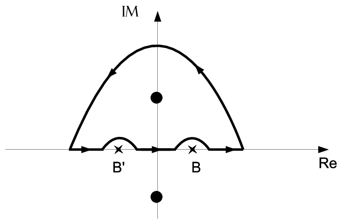
Refer to caption
Figure 1: Integration contour for Eq. (127). The lower order poles, which are a pure imaginary number, are indicated by the d ot symbol ∙\bullet. The higher order poles has only a real part, as indicated by the X symbol and their contribution is a pure imaginary number.
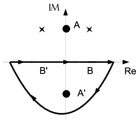
Refer to caption
Figure 2: This figure illustrated the easiest integration contour we may choose to evaluate Eq. (128). It is easiest because we avoid the highest order poles represented by the symbol X in the figure. So the contribution of I2I_{2} integral is only due to the negative and imaginary lower order pole which is indicated by the dot symbol ∙\bullet in the lower half plane.

In order to do that, let us choose a contour that avoids the third order poles located in the real axis at η1=±r+η2\eta_{1}=\pm r+\eta_{2} (as indicated, in Fig. (1), by the letters BB and B′B^{{}^{\prime}}). Then, we evaluate the integral considering only one of the second order poles, namely, η1=±i​η0\eta_{1}=\pm i\eta_{0}. In Fig. (1) we illustrate only the contour in the upper half plane. The contour in the lower half plane would give us the same answer, according to the residue theorem. So the first integral (I1)(I_{1}) has the form

I1=η0​(G2−1)2​[−(η2−i​η0)2−r2]2​π​[−(η2−i​η0)2+r2]3+2​η0​(G2−1)​[−(η2−i​η0)2−r2]π2​[−(η2−i​η0)2+r2]3\displaystyle I_{1}=\frac{\eta_{0}(G^{2}-1)^{2}[-(\eta_{2}-i\eta_{0})^{2}-r^{2}]}{2\pi[-(\eta_{2}-i\eta_{0})^{2}+r^{2}]^{3}}+\frac{2\eta_{0}(G^{2}-1)[-(\eta_{2}-i\eta_{0})^{2}-r^{2}]}{\pi^{2}[-(\eta_{2}-i\eta_{0})^{2}+r^{2}]^{3}}
−3​η02​i​(η2−i​η0)​(G2−1)2π​[−(η2−i​η0)2+r2]3+3​η0​i​(G2−1)​(η2−i​η0)​[−(η2−i​η0)2−r2]π​[−(η2−i​η0)2−r2]4.\displaystyle-\frac{3\eta_{0}^{2}i(\eta_{2}-i\eta_{0})(G^{2}-1)^{2}}{\pi[-(\eta_{2}-i\eta_{0})^{2}+r^{2}]^{3}}+\frac{3\eta_{0}i(G^{2}-1)(\eta_{2}-i\eta_{0})[-(\eta_{2}-i\eta_{0})^{2}-r^{2}]}{\pi[-(\eta_{2}-i\eta_{0})^{2}-r^{2}]^{4}}.

Now the second integral is

I2=∫−∞+∞d​η2​(η22+G2​η02η22+η02)2​I1.I_{2}=\int^{+\infty}_{-\infty}d\eta_{2}\left(\frac{\eta_{2}^{2}+G^{2}\eta_{0}^{2}}{\eta_{2}^{2}+\eta_{0}^{2}}\right)^{2}I_{1}. (128)

The integrand in I2I_{2} has a second order pole located at η2=±i​η0\eta_{2}=\pm i\eta_{0} and three third and one fourth orders poles at η2=±i​η0\eta_{2}=\pm i\eta_{0}. We evaluate I2I_{2} in the lower half plane to avoid the highest order poles, as indicated in Fig. (2). Even if we had chosen a contour in the upper half plane, our answer would be the same, but the way to do that would be harder. So, the final result for the mean squared velocity (OPEN⟨Δ​u​(r1)​Δ​u​(r2)⟩=q2m2​I1​I2)\langle\Delta u(r_{1})\Delta u(r_{2})\rangle=\frac{q^{2}}{m^{2}}I_{1}I_{2}) is,

⟨Δ​u​(r1)​Δ​u​(r2)⟩=q2​η0​Θ2m2​{η0​Θ2​(12​η02−r′2)(4​η02+r2)3+η0​Θ​(12​η02−r′2)(4​η02+r2)3}\displaystyle\langle\Delta u(r_{1})\Delta u(r_{2})\rangle=\frac{q^{2}\eta_{0}\Theta^{2}}{m^{2}}\left\{\frac{\eta_{0}\Theta^{2}(12\eta_{0}^{2}-r^{\prime 2})}{(4\eta_{0}^{2}+r^{2})^{3}}+\frac{\eta_{0}\Theta(12\eta_{0}^{2}-r^{\prime 2})}{(4\eta_{0}^{2}+r^{2})^{3}}\right\} (129)
+q2​η0​Θ2m2​{−3​η03​Θ2(4​η02+r2)3+3​η03​Θ​(12​η02−r′2)(4​η02+r2)4}\displaystyle+\frac{q^{2}\eta_{0}\Theta^{2}}{m^{2}}\left\{\frac{-3\eta_{0}^{3}\Theta^{2}}{(4\eta_{0}^{2}+r^{2})^{3}}+\frac{3\eta_{0}^{3}\Theta(12\eta_{0}^{2}-r^{\prime 2})}{(4\eta_{0}^{2}+r^{2})^{4}}\right\}
+4​q2​η0​Θm2​{η0​Θ2​(12​η02−r′2)(4​η02+r2)3+η0​Θ​(12​η02−r′2)(4​η02+r2)3}\displaystyle+\frac{4q^{2}\eta_{0}\Theta}{m^{2}}\left\{\frac{\eta_{0}\Theta^{2}(12\eta_{0}^{2}-r^{\prime 2})}{(4\eta_{0}^{2}+r^{2})^{3}}+\frac{\eta_{0}\Theta(12\eta_{0}^{2}-r^{\prime 2})}{(4\eta_{0}^{2}+r^{2})^{3}}\right\}
+4​q2​η0​Θm2​{−3​η03​Θ2(4​η02+r2)3+3​η03​Θ2​(12​η02−r′2)(4​η02+r2)4}\displaystyle+\frac{4q^{2}\eta_{0}\Theta}{m^{2}}\left\{\frac{-3\eta_{0}^{3}\Theta^{2}}{(4\eta_{0}^{2}+r^{2})^{3}}+\frac{3\eta_{0}^{3}\Theta^{2}(12\eta_{0}^{2}-r^{\prime 2})}{(4\eta_{0}^{2}+r^{2})^{4}}\right\}
−q2​η02​Θ2m2​{3​η02​Θ22​(4​η02+r2)3−3​η02​Θ​(12​η02−r′2)(4​η02+r2)4}\displaystyle-\frac{q^{2}\eta_{0}^{2}\Theta^{2}}{m^{2}}\left\{\frac{3\eta_{0}^{2}\Theta^{2}}{2(4\eta_{0}^{2}+r^{2})^{3}}-\frac{3\eta_{0}^{2}\Theta(12\eta_{0}^{2}-r^{\prime 2})}{(4\eta_{0}^{2}+r^{2})^{4}}\right\}
−q2​η02​Θ2m2​{12​η02​Θ(4​η02+r2)3+12​η02​Θ​(12​η02−r′2)(4​η02+r2)4}\displaystyle-\frac{q^{2}\eta_{0}^{2}\Theta^{2}}{m^{2}}\left\{\frac{12\eta_{0}^{2}\Theta}{(4\eta_{0}^{2}+r^{2})^{3}}+\frac{12\eta_{0}^{2}\Theta(12\eta_{0}^{2}-r^{\prime 2})}{(4\eta_{0}^{2}+r^{2})^{4}}\right\}
−q2​η02​Θ2m2​{72​η04​Θ2(4​η02+r2)4−48​η04​Θ​(12​η02−r′2)(4​η02+r2)5}\displaystyle-\frac{q^{2}\eta_{0}^{2}\Theta^{2}}{m^{2}}\left\{\frac{72\eta_{0}^{4}\Theta^{2}}{(4\eta_{0}^{2}+r^{2})^{4}}-\frac{48\eta_{0}^{4}\Theta(12\eta_{0}^{2}-r^{\prime 2})}{(4\eta_{0}^{2}+r^{2})^{5}}\right\} ,

where Θ≡G2−1\Theta\equiv G^{2}-1.

B.2 Evaluation of Eq. (56)

Next we turn to the evaluation of Eq (56). Define a new I1I_{1} integral as

I1=∫−∞+∞d​η1​(1a02+a12​tanh⁡(η1η0))​[−(η2−η1)2−r2′π2​[−(η2−η1)2+r2]3].I_{1}=\int_{-\infty}^{+\infty}d\eta_{1}\left(\frac{1}{a_{0}^{2}+a_{1}^{2}\tanh\left(\frac{\eta_{1}}{\eta_{0}}\right)}\right)\left[\frac{-(\eta_{2}-\eta_{1})^{2}-r^{{}^{\prime}2}}{\pi^{2}[-(\eta_{2}-\eta_{1})^{2}+r^{2}]^{3}}\right]\,. (130)

We see that in the η1\eta_{1} integral we have third order poles located in the real axis at: η1=±r+η2\eta_{1}=\pm r+\eta_{2}, and an infinite number of poles at tanh⁡(η1/η0)=−α2\tanh(\eta_{1}/\eta_{0})=-\alpha^{2}, where α2≡a02/a12>1\alpha^{2}\equiv a_{0}^{2}/a_{1}^{2}>1. These are the first order poles, and can be written as

η1​k=η10+12​(2​k+1)​i​π​η0,\eta_{1k}=\eta_{10}+\frac{1}{2}(2k+1)i\pi\eta_{0}, (131)

with k=0,±1,±2,…k=0,\pm 1,\pm 2,..., and η10=−π​i2​η0−12​η0​ln⁡(α2+1α2−1)\eta_{10}=-\frac{\pi i}{2}\eta_{0}-\frac{1}{2}\eta_{0}\ln\left(\frac{\alpha^{2}+1}{\alpha^{2}-1}\right).

Following the contour indicated in Fig. (3) we obtain,

I1=∑k=1∞2​i​η0​cosh2⁡(η1​kη0)a12​[−(η2−η1​k)2−r2′π​[−(η2−η1​k)2+r2]3],I_{1}=\sum_{k=1}^{\infty}\frac{2i\eta_{0}\cosh^{2}\left(\frac{\eta_{1k}}{\eta_{0}}\right)}{a_{1}^{2}}\left[\frac{-(\eta_{2}-\eta_{1k})^{2}-r^{{}^{\prime}2}}{\pi[-(\eta_{2}-\eta_{1k})^{2}+r^{2}]^{3}}\right], (132)

Note that a contour in the lower half plane would give us the same answer. With this result, the η2\eta_{2} integral turns into

Refer to caption
Figure 3: One possible contour to integrate Eq. (130). We avoid the higher order poles, indicated by X symbol, because their contribution is a pure imaginary number. The contour is, however, an infinity contour that encloses the infinity positives lower order poles which are indicated by the symbol ∙\bullet.
I2=∑k=1∞2​i​η0a12​cosh2⁡(η1​kη0)​∫−∞+∞d​η2a02+a12​tanh⁡(η2η0)\displaystyle I_{2}=\sum_{k=1}^{\infty}\frac{2i\eta_{0}}{a_{1}^{2}}\cosh^{2}\left(\frac{\eta_{1k}}{\eta_{0}}\right)\int_{-\infty}^{+\infty}\frac{d\eta_{2}}{a_{0}^{2}+a_{1}^{2}\tanh\left(\frac{\eta_{2}}{\eta_{0}}\right)} (133)
×[−(η2−η1​k)2−r2′π​[−(η2−η1​k)2+r2]3].\displaystyle\times\left[\frac{-(\eta_{2}-\eta_{1k})^{2}-r^{{}^{\prime}2}}{\pi[-(\eta_{2}-\eta_{1k})^{2}+r^{2}]^{3}}\right].

It has third order poles, but now located at, η2=±r+η1​k\eta_{2}=\pm r+\eta_{1k}, and first order poles at η2​l=η20+12​(2​l+1)​i​π​η0\eta_{2l}=\eta_{20}+\frac{1}{2}(2l+1)i\pi\eta_{0}, with η20=η10\eta_{20}=\eta_{10}, and l=0,±1,±2,l=0,\pm 1,\pm 2, …These singularities are located in the complex plane as indicated in Fig. (4). To avoid the third order poles we choose a contour in the lower half plane, however the same answer is required if we had chosen the contour in the upper plane.

Refer to caption
Figure 4: The figure shows the easiest possible contour to integrate Eq. (133), because the infinities higher order poles (the X symbol) are excluded. The enclosed poles are the infinities lower orders, which are indicated by ∙\bullet symbol.

So our result is,

⟨Δ​u​(r1)​Δ​u​(r2)⟩=−4​η02a14​sinh4⁡[12​ln⁡(α2+1α2−1)]​S,\langle\Delta u(r_{1})\Delta u(r_{2})\rangle=-4\frac{\eta_{0}^{2}}{a_{1}^{4}}\sinh^{4}\left[\frac{1}{2}\ln\left(\frac{\alpha^{2}+1}{\alpha^{2}-1}\right)\right]\;S\,, (134)

where

S=∑k=1∞∑l′=1∞[π2(l′+k)2η02−r2[π2(l′+k)2η02+r2]3]=∑j=2∞(j−1)π2​j2​η02−r2[π2​j2​η02+r2]3.S=\sum_{k=1}^{\infty}\sum_{l^{{}^{\prime}}=1}^{\infty}\left[\frac{\pi^{2}(l^{{}^{\prime}}+k)^{2}\eta_{0}^{2}-r^{2}}{[\pi^{2}(l^{{}^{\prime}}+k)^{2}\eta_{0}^{2}+r^{2}]^{3}}\right]=\sum_{j=2}^{\infty}(j-1)\frac{\pi^{2}j^{2}\eta_{0}^{2}-r^{2}}{[\pi^{2}j^{2}\eta_{0}^{2}+r^{2}]^{3}}. (135)

In the second form we transformed the double sum into a single sum by defining j≡k+l′−1j\equiv k+l^{{}^{\prime}}-1 and l′≡−ll^{{}^{\prime}}\equiv-l. This sum can be evaluated explicitly to yield

S=1π4​η04​[−i​π​η02​r​Ψ​(1,2−i​rη0​π)+i​π​η02​r​Ψ​(2,2+i​rη0​π)]\displaystyle S=\frac{1}{\pi^{4}\eta_{0}^{4}}\left[-\frac{i\pi\eta_{0}}{2r}\Psi\left(1,2-\frac{ir}{\eta_{0}\pi}\right)+\frac{i\pi\eta_{0}}{2r}\Psi\left(2,2+\frac{ir}{\eta_{0}\pi}\right)\right] (136)
+1π4​η04​[(−14−i​π​η04​r)​Ψ​(2,2−i​rη0​π)+(−14+i​π​η04​r)​Ψ​(2,2+i​rη0​π)],\displaystyle+\frac{1}{\pi^{4}\eta_{0}^{4}}\left[\left(-\frac{1}{4}-\frac{i\pi\eta_{0}}{4r}\right)\Psi\left(2,2-\frac{ir}{\eta_{0}\pi}\right)+\left(-\frac{1}{4}+\frac{i\pi\eta_{0}}{4r}\right)\Psi\left(2,2+\frac{ir}{\eta_{0}\pi}\right)\right],

where Ψ⁡(n,x)\Psi(n,x) is the nth Polygamma function (This calculation was done using the algebraic program, Maple).

B.3 Evaluation of Eq. (76)

Let the I1I_{1} integral in the variable η1\eta_{1}. We may evaluate it using again the residue theorem. The η1\eta_{1} integral has third order poles at η1=±r+η2\eta_{1}=\pm r+\eta_{2}, and single poles at η1=±i​η0\eta_{1}=\pm i\eta_{0}. Here, we can use again the integration contour in Fig. (1). However, the symbol ∙\bullet represents singles order poles and not second order poles as in the case of Eq. (127) which corresponds to the asymptotically flat bouncing universe. Thus, the integral I1I_{1} is expressed as,

I1=∫−∞+∞d​η1​(1H2​η12+H2​η02)​[−(η2−η1)2−r2π2​[−(η2−η1)2+r2]3]\displaystyle I_{1}=\int_{-\infty}^{+\infty}d\eta_{1}\left(\frac{1}{H^{2}\eta_{1}^{2}+H^{2}\eta_{0}^{2}}\right)\left[\frac{-(\eta_{2}-\eta_{1})^{2}-r^{2}}{\pi^{2}[-(\eta_{2}-\eta_{1})^{2}+r^{2}]^{3}}\right] (137)
=−(η2−i​η0)2−r2η0​H2​[−(η2−i​η0)2+r2]3.\displaystyle=\frac{-(\eta_{2}-i\eta_{0})^{2}-r^{2}}{\eta_{0}H^{2}[-(\eta_{2}-i\eta_{0})^{2}+r^{2}]^{3}}.

The η2\eta_{2} integral is given by

I2=∫−∞+∞1H2​η2+H2​η02​I1.I_{2}=\int^{+\infty}_{-\infty}\frac{1}{H^{2}\eta^{2}+H^{2}\eta_{0}^{2}}I_{1}. (138)

It has two single poles at η2=±i​η0\eta_{2}=\pm i\eta_{0} and two third order poles at η2=±r+i​η0\eta_{2}=\pm r+i\eta_{0}. In this case we choose a contour in the lower half plane, as in the Fig. (2), with the symbol ∙\bullet representing now first order poles. This contour avoids the third order poles. Even if we choose the contour in the upper half plane, our result would be the same. Then, after the integrations Eq. (138) results in

⟨Δ​u​(r1)​Δ​u​(r2)⟩=q2m2​[3​η02−r2η02​H4​[4​η02+r2]3].\langle\Delta u(r_{1})\Delta u(r_{2})\rangle=\frac{q^{2}}{m^{2}}\left[\frac{3\eta_{0}^{2}-r^{2}}{\eta_{0}^{2}H^{4}[4\eta_{0}^{2}+r^{2}]^{3}}\right]. (139)

B.4 Evaluation of Eq. (93)

Next we consider the evaluation of Eq. (93). The η1\eta_{1} singularities has third order poles located at η1=±r+η2\eta_{1}=\pm r+\eta_{2}, and first order poles at cos⁡(ω​η1)=−α2​η12−α2​η02\cos(\omega\eta_{1})=-\alpha^{2}\eta_{1}^{2}-\alpha^{2}\eta_{0}^{2}, where α2≡a02/a12\alpha^{2}\equiv a_{0}^{2}/a_{1}^{2} or η1​k=−iω​ln⁡(α2​B​(η1​k)+α2​B​(η1​k)−1)+12​(2​k+1)​πω\eta_{1k}=-\frac{i}{\omega}\ln\left(\alpha^{2}B(\eta_{1k})+\sqrt{\alpha^{2}B(\eta_{1k})-1}\right)+\frac{1}{2}(2k+1)\frac{\pi}{\omega}, with k=0,±1,±2,k=0,\pm 1,\pm 2, …, and B⁡(η1​k≡η12+η02)B(\eta_{1k}\equiv\eta_{1}^{2}+\eta_{0}^{2}). These singularities are located as indicated in Fig. (5), with the X symbol now representing the third order poles and the several ⋅⋯⋅\cdot\cdot\cdot\cdot\cdot symbols representing the infinities numbers of first order poles. So apparently, this integral is zero because we do not have any poles enclosed by one of the possible contours. However, if η=i​x\eta=ix, we can find two real poles in the integrand, because cos⁡(ω​η1)=−α2​η12−α2​η02⇒cosh⁡(ω​x)=−α2​x2−α2​η02\cos(\omega\eta_{1})=-\alpha^{2}\eta_{1}^{2}-\alpha^{2}\eta_{0}^{2}\Rightarrow\cosh(\omega x)=-\alpha^{2}x^{2}-\alpha^{2}\eta_{0}^{2}.

Refer to caption
Figure 5: This figure shows that it is possible to choose one contour where the integral is apparently null.
Refer to caption
Figure 6: This figure shows that Eq. (93) has at least one imaginary pole located at η0\eta_{0} which can be enclosed by the contour of Fig. (5).

Now we have the picture indicated in Fig. (6). Then, we have at least one contribution due the imaginary first order pole represented there by the symbol ∙\bullet. Thus, the η1\eta_{1} integral (I1I_{1}) is,

I1=22​a02​x−a12​ω​sinh⁡(x​ω)​[−3​(η2−i​x)2−r2′π​[−(η2−i​x)2+r2]3],I_{1}=\frac{2}{2a_{0}^{2}x-a_{1}^{2}\omega\sinh(x\omega)}\left[\frac{-3(\eta_{2}-ix)^{2}-r^{{}^{\prime}2}}{\pi[-(\eta_{2}-ix)^{2}+r^{2}]^{3}}\right], (140)

and the I2I_{2} is defined as:

I2=22​a02​x−a12​ω​sinh⁡(x​ω)​∫−∞+∞d​η2a02​η22+a02​η02+a12​cos⁡(ω​η2)\displaystyle I_{2}=\frac{2}{2a_{0}^{2}x-a_{1}^{2}\omega\sinh(x\omega)}\int^{+\infty}_{-\infty}\frac{d\eta_{2}}{a_{0}^{2}\eta_{2}^{2}+a_{0}^{2}\eta_{0}^{2}+a_{1}^{2}\cos(\omega\eta_{2})} (141)
×[−3​(η2−i​x)2−r2′π​[−(η2−i​x)2+r2]3].\displaystyle\times\left[\frac{-3(\eta_{2}-ix)^{2}-r^{{}^{\prime}2}}{\pi[-(\eta_{2}-ix)^{2}+r^{2}]^{3}}\right].

To treat these poles, we should proceed as in the case of the first integral, as indicated in Fig. (7). Now the poles are located at η2=±r+i​x\eta_{2}=\pm r+ix (third order), and at η2=±i​x\eta_{2}=\pm ix (first order). Thus, we obtain the result,

I2=−4r4​[2​a02​x−a12​ω​sinh⁡(ω​x)]+2​i2​a02​x−a12​ω​sinh⁡(ω​x)​Θ,\displaystyle I_{2}=\frac{-4}{r^{4}[2a_{0}^{2}x-a_{1}^{2}\omega\sinh(\omega x)]}+\frac{2i}{2a_{0}^{2}x-a_{1}^{2}\omega\sinh(\omega x)}\Theta, (142)

where Θ\Theta is given by:

Refer to caption
Figure 7: This figure shows the easiest possible contour we can choose to integrate Eq. (141). Here the symbol ∙\bullet represents the first order poles located at i​xix, the X represents the third order poles, and ⋅⋯\cdot\cdot\cdot\cdot the infinity first order poles at OPENη1​k=−iω​ln⁡(α2​B​(η1​k)+α2​B​(η1​k)−1))+12​(2​k+1)​πω\eta_{1k}=-\frac{i}{\omega}\ln\left(\alpha^{2}B(\eta_{1k})+\sqrt{\alpha^{2}B(\eta_{1k})-1})\right)+\frac{1}{2}(2k+1)\frac{\pi}{\omega}.
Θ≡\displaystyle\Theta\equiv −{2​a02​(−r′+i​x)−a12​ω​sinh⁡[ω⁡(−r′+i​x)]}2r​{a02​(−r+i​x)2+a02​η02+a12​cos⁡[ω⁡(−r+i​x)]}3\displaystyle\frac{-\{2a_{0}^{2}(-r^{\prime}+ix)-a_{1}^{2}\omega\sinh[\omega(-r^{\prime}+ix)]\}^{2}}{r\{a_{0}^{2}(-r+ix)^{2}+a_{0}^{2}\eta_{0}^{2}+a_{1}^{2}\cos[\omega(-r+ix)]\}^{3}} (143)
+2​a02−a12​ω2​cos⁡[ω⁡(−r′+i​x)]2​r​{a02​(−r+i​x)2+a02​η02+a12​cos⁡[ω⁡(−r+i​x)]}2\displaystyle+\frac{2a_{0}^{2}-a_{1}^{2}\omega^{2}\cos[\omega(-r^{\prime}+ix)]}{2r\{a_{0}^{2}(-r+ix)^{2}+a_{0}^{2}\eta_{0}^{2}+a_{1}^{2}\cos[\omega(-r+ix)]\}^{2}}
+{2​a02​(r′+i​x)−a12​ω​sinh⁡[ω⁡(r′+i​x)]}2r​{a02​(r+i​x)2+a02​η02+a12​cos⁡[ω⁡(r+i​x)]}3\displaystyle+\frac{\{2a_{0}^{2}(r^{\prime}+ix)-a_{1}^{2}\omega\sinh[\omega(r^{\prime}+ix)]\}^{2}}{r\{a_{0}^{2}(r+ix)^{2}+a_{0}^{2}\eta_{0}^{2}+a_{1}^{2}\cos[\omega(r+ix)]\}^{3}}
+−{2​a02−a12​ω2​cos⁡[ω⁡(r′+i​x)]}2​r​{a02​(r+i​x)2+a02​η02+a12​cos⁡[ω⁡(r+i​x)]}2.\displaystyle+\frac{-\{2a_{0}^{2}-a_{1}^{2}\omega^{2}\cos[\omega(r^{\prime}+ix)]\}}{2r\{a_{0}^{2}(r+ix)^{2}+a_{0}^{2}\eta_{0}^{2}+a_{1}^{2}\cos[\omega(r+ix)]\}^{2}}.

In order to check if our answer is correct, let us take a1≃0a_{1}\simeq 0 and x=η0x=\eta_{0}. Then we obtain,

I2=4​η02−r′2η02​a04​[4​η02+r2]3,I_{2}=\frac{4\eta_{0}^{2}-r^{\prime 2}}{\eta_{0}^{2}a_{0}^{4}[4\eta_{0}^{2}+r^{2}]^{3}}, (144)

which is the same answer we found in the bouncing case Eq. (139). Now, using the smallest power terms in a1a_{1} and r≪η0r\ll\eta_{0}, we have the squared coordinate velocity written as,

⟨Δ​u​(r1)​Δ​u​(r2)⟩≅q2m2​[316​a04​η06+a122​a06​r4​η03​(3​ω​sinh⁡(ω​η0)+cosh⁡(ω​η0)η0)],\langle\Delta u(r_{1})\Delta u(r_{2})\rangle\cong\frac{q^{2}}{m^{2}}\left[\frac{3}{16a_{0}^{4}\eta_{0}^{6}}+\frac{a_{1}^{2}}{2a_{0}^{6}r^{4}\eta_{0}^{3}}\left(3\omega\sinh(\omega\eta_{0})+\frac{\cosh(\omega\eta_{0})}{\eta_{0}}\right)\right], (145)

and when nf≫n0n_{f}\gg n_{0}, ⟨Δ​v​(r1)​Δ​v​(r2)⟩\langle\Delta v(r_{1})\Delta v(r_{2})\rangle is given by Eq. (94).

References

  • [1] R.K. Pathria, Statistical Mechanics, (Pergamon,Oxford, 1972), Chap. 13.
  • [2] G. Gour and L. Sriramkumar, Foundations of Physics 29, 1917 (1999).
  • [3] G. Barton, J. Phys. A24, 991 (1991); A24, 5563 (1991).
  • [4] M. T. Jaekel and S. Reynaud, Quantum Opt. 4, 39 (1992); J. Phys. I (France) 2, 149 (1992); 3, 1 (1993); 3, 339 (1993).
  • [5] C-H. Wu, C-I Kuo and L. H. Ford, Phys. Rev. A65, 062102 (2002).
  • [6] H. Yu and L. H. Ford, Phys. Rev. D70, 065009 (2004).
  • [7] C-H. Wu and D-S. Lee, Phys. Rev. D71, 125005 (2005).
  • [8] M. Seriu and C-H. Wu, arXiv:0711.2203
  • [9] H. B. G. Casimir and D. Polder, Phys. Rev. 73, 360 (1948).
  • [10] L. H. Ford, Int. J. Theor. Phys. 46, 2218 (2007), quant-ph/0601112.
  • [11] L. H. Ford and T. A. Roman, Phys. Rev. D72, 105010 (2005).
  • [12] L. H. Ford, Ann. Phys. 144, 238 (1982).
  • [13] C-I Kuo and L. H. Ford, Phys. Rev. D47, 4510 (1993).
  • [14] L. H. Ford, Int. J. Theor. Phys. 44, 1753, (2005).
  • [15] L. H. Ford and N. F. Svaiter, Phys. Rev. D54, 2640 (1996).
  • [16] L. H. Ford and N. F. Svaiter, Phys. Rev. D56, 2226 (1997).
  • [17] Y. J. Ng and H. van Dam, Phys. Lett. B477, 429 (2000).
  • [18] G. Amelino-Camelia, Nature 398, 216 (1999).
  • [19] E. Calzetta and B. L. Hu, Phys. Rev. D49, 6636 (1993); Phys. Rev. D52, 6770 (1995).
  • [20] E. Calzetta, A. Campos and E. Verdaguer, Phys. Rev. D56, 2163 (1997).
  • [21] M. Novello, V. B. Bezerra and V. M. Mostepanenko, Int. J. Mod. Phys. 7, 779 (1998).
  • [22] R. Martin and E. Verdaguer, Phys. Rev. D60, 084008 (1999).
  • [23] B. L. Hu and K. Shiokawa, Phys. Rev. D57, 3474 (1998).
  • [24] R. T. Thompson and L. H. Ford, Phys.Rev. D74, 024012, (2006).
  • [25] C-H Wu, K-W Ng and L. H. Ford, Phys.Rev. D75, 103502, (2007).
  • [26] J. Audretsch and G. Schäfer, Phys. Let. A66, 459 (1978).
  • [27] C. Bernard and A. Duncan. Ann. Phys. 107, 201 (1977).
  • [28] A. Tomimatsu and H. Ishihara, Gen. Rel. Grav. 18, 161 (1986).
  • [29] A. Guth, Phys. Rev. D23, 347 (1981).
  • [30] A. Linde, hep-th/07050164.
  • [31] G. Börner, The Early Universe, Facts and Fiction (Springer-Verlag Berlin Heidelberg) 2003.
  • [32] A. R. Liddle and D. H. Lyth, Cosmological Inflation and Large-Scale Structure (Cambridge University Press) 2000.
  • [33] D. N. Spergel et al, astro-ph/0603449.
  • [34] W. G. Unruh, Phys. Rev. D14, 870 (1976).
  • [35] L. Parker, Phys. Rev. 183, 1057 (1969).
  • [36] E. W. Kolb, D. J. H. Chung and A. Riotto, hep-ph/9810361; H. Ziaeepour, Astropart. Phys. 16, 101 (2001); E. W. Kolb, A. A. Starobinsky and I. I. Tkachev, hep-th/0702143.
  • [37] D. J. H. Chung, E. W. Kolb, and A. Riotto, Phys. Rev. Lett. 81, 4048 (1998); Phys. Rev. D59, 023501 (1999); D. J. H. Chung, Phys. Rev. D67, 083514 (2003); D. J. H. Chung, P. Crotty, E. W. Kolb, and A. Riotto, Phys. Rev. D64, 043503 (2001); D. J. H. Chung, E. W. Kolb, A. Riotto, and L. Senatore, Phys. Rev. D72, 023511 (2005).
  • [38] L. H. Ford, Phys. Rev. D35, 2955 (1987).